Gamma-delayed deuteron emission of the ⁶Li$(0^{+};T=1)$ halo state

The ⁶Li bound-state wave functions are defined in an $\alpha+n+p$ model using the hyperspherical coordinates [5]. A set of Jacobi coordinates for three particles with mass numbers $A_{1}=1$, $A_{2}=1$, and $A_{3}=4$ is defined as

where the (dimensionless) reduced masses are given by $\mu_{pn}=1/2$ and $\mu_{\alpha d}=4/3$. The $p-n$ relative coordinate and the coordinate between $\alpha$ and $d$ are denoted by $r$ and $R$, respectively. Equations (1) define six coordinates which are transformed to the hyperspherical coordinates as

where $\alpha$ varies between 0 and $\pi/2$. With the angular variables $\Omega_{x}=(\theta_{x},\varphi_{x})$ and $\Omega_{y}=(\theta_{y},\varphi_{y})$, equations (2) define a set of hyperspherical coordinates which are known to be well adapted to the three-body Schrödinger equation.

We define $\gamma=(\ell_{x},\ell_{y},L,S)$ where $\ell_{x}$ and $\ell_{y}$ are the orbital momenta associated with the Jacobi coordinates $x$ and $y$, respectively. With the notation $\Omega_{5}=(\alpha,\Omega_{x},\Omega_{y})$, a three-body wave function with spin $J$ and parity $\pi$ reads [6]

where ${\cal Y}^{JM}_{\gamma K}(\Omega_{5})$ are the hyperspherical functions (including spin), defined as

with $n=(K-\ell_{x}-\ell_{y})/2$, and where ${\cal N}_{K}^{\ell_{x}\ell_{y}}$ is a normalization factor, $P_{n}^{a,b}$ a Jacobi polynomial and ${\chi}^{S}$ a spin function. Details are given in Refs. [5, 6]. The hyperradial functions ${\chi}^{J\pi}_{\gamma K}$ are obtained from a set of coupled equations truncated at $K=K_{max}$. The problem is solved by using the Lagrange-mesh technique (see Ref. [6] for details).

The three-body wave functions contain components with total intrinsic spin $S=0$ and $S=1$. Because of the positive parity, $\ell_{x}+\ell_{y}$ is even and only even $K$ values are involved.

As it was done in Ref. [4] for the ⁶He $\beta$ decay, the scattering $\alpha+d$ wave functions are factorized into a deuteron ground-state wave function, calculated with an appropriate NN potential, and an $\alpha+d$ wave function derived from a potential model. We neglect the small $D$ component of the deuteron. In the $\alpha+d$ exit channel, only $S$ waves are involved. Consequently, the final $1^{+}$ wave function reads

The spatial part of the deuteron wave function is written as

The $S$-wave component of the $\alpha+d$ relative motion wave function is factorized as

The normalization of the scattering wave function is fixed by the asymptotic behaviour as

where $F_{0}$ and $G_{0}$ are the Coulomb functions, $\delta_{0}(E)$ is the $s$-wave phase shift at energy $E$, and $k_{\alpha d}$ is the wave number of the relative motion.

The present two-body model can also be applied to $\alpha+d$ bound states. In that case, the scattering wave function $u_{E}(R)$ in Eq. (7) is replaced by an $S$-wave bound-state radial function.

For the M1 transition to the ground state, the gamma width is calculated from

where $k_{\gamma}$ is the wave number of the emitted photon. This definition involves bound-state wave functions on both sides.

With the normalization (8) of the scattering wave function, the M1 transition probability of the process

per time and energy units, is given by reduced matrix elements between the initial bound state and the final scattering states as (see Appendix A)

where $m_{N}$ is the nucleon mass. The maximum $\alpha+d$ energy is $Q=2.089$ MeV. The M1 differential gamma width per energy unit to continuum states is expressed as

and the total width is deduced by integration over the energy.

The M1 operator contains orbital and spin-dependent components. For a general three-body system, it reads, in Jacobi coordinates [6]

where $\mu_{N}=e\hbar/m_{N}c$ is the nuclear magneton, ${\mbox{\boldmath$s$}}_{i}$ are the spins of the three particles, and $g_{s}(i)$ their gyromagnetic factors. Coefficients $A_{x}$, $A_{y}$ and $A_{xy}$ are related to the mass and charge numbers as

where $A_{12}$ is the reduced mass of the $1+2$ system; in the present case it is denoted as $\mu_{pn}$. Variables $p_{x}$ and $p_{y}$ are the momenta associated with the Jacobi coordinates $x$ and $y$, respectively. The matrix elements of the M1 operator between hyperspherical functions are given in Appendix B.

A test of three-body wave functions is provided by M1 spectroscopic properties, which are well known experimentally [15]. In Table 1, we present the calculated values of the magnetic moment and of the B(M1) in ⁶Li. Separate contributions are given for the orbital and spin terms of the M1 operator [see Eq. (13)]. In both cases, the contribution of the orbital term is small since the dominant component in the ground-state wave function is an $S$ wave. The main contribution to the M1 matrix element comes from the spin term. The present matrix element corresponds to $B(M1)=7.9$ W.u., or $\Gamma_{\gamma}=7.5$ eV, which are in good agreement with experiment ($8.62\pm 0.18$ W.u. and $8.19\pm 0.17$ eV, respectively). The results are also close to those of Kukulin et al. [16] who use different variants of a three-body model.

These matrix elements can also be obtained with a 2-body description of the ⁶Li ground state. In that case we use the potential $V_{a}$ to generate the wave functions. Since components with $L\neq 0$ are small in the ground-state wave function, the two-body model is expected to be a good approximation. The $1^{+}$ magnetic moment in the two-body model is a simple sum of the proton and neutron magnetic moments. In this case, both approaches provide similar results, in good agreement with experiment. However the rms radius in the two-body model is $\sqrt{<r^{2}>}=2.11$ fm, lower than experiment and than the three-body value (see Sect.3.1.1). In addition, the M1 transition matrix element (see Table 1) provides $\Gamma_{\gamma}=3.9$ eV, i.e. an underestimate of the experimental value. These results suggest that the short-range part of the two-body description is too simple. However, transitions to the continuum are more sensitive to the long-range part of the $\alpha-d$ wave functions.

Since the $\alpha+d$ relative motion is described by $S$ waves, the first and second orbital terms of the M1 transition operator (13) do not contribute to the reduced matrix elements for transitions to the $\alpha+d$ continuum. The orbital and spin terms yield nonzero matrix elements only for the $\ell_{x}=\ell_{y}=L=S=1$ and $\ell_{x}=\ell_{y}=L=S=0$ components of the three-body wave function, respectively. As it will be shown further, the main contribution comes from the spin part of the transition operator. The $P$-wave hyperspherical components give small corrections to the process since the $0^{+}$ state is essentially $S=0$.

In order to analyze the $\gamma$-decay process to the continuum, we introduce effective wave functions and their integrals, in analogy with the $\beta$-decay study of the ⁶He halo nucleus into the $\alpha+d$ continuum [4]. We restrict the presentation to the dominant spin part. For the initial $0^{+}$ state, let us define the effective wave function with hypermomentum $K$

and the effective integrals

where $\rho$ and $\alpha$ depend on $(r,R)$, as given in Eq. (2). The normalization factor in Eq. (15) arises from the Jacobian between the $(\mbox{\boldmath$R$},\mbox{\boldmath$r$})$ and $(\mbox{\boldmath$x$},\mbox{\boldmath$y$})$ coordinates. The reduced matrix elements of the M1 operator (spin part) are then directly proportional to $I_{E}(R)$ (see Appendix B).

In the following, we analyze two properties: the convergence of the hypermomentum expansion, and the sensitivity of the effective integrals with respect to the $\alpha+d$ potential. Let us start with the influence of $K_{\rm max}$. In Fig. 2 we show the integrals $I_{E}^{(K)}(R)$ calculated at $E=1$ MeV with potential $V_{a}$, for different $K$-values. The dominant contribution at large $R$ values comes from the $K=0,2,8$ components in the ⁶Li$(0^{+})$ wave function. The components $K=4$ and $K=10$ give smaller and comparable effects to the process. The contributions of other components are small and not visible at the scale of the figure. Similar results were obtained for the $\beta$ decay of ⁶He [4]. In Ref. [4] it was shown that the $K=4$ and $K=6$ contributions are affected by cancellation effects, which do not occur for $K\geq 8$. The situation is therefore very close to the ⁶He$(0^{+})$ beta decay [4] into the $\alpha+d$ continuum which confirms the halo structure of the ⁶Li$(0^{+})$ state, suggested by its large r.m.s. radius.

In the second step, we analyze the sensitivity of the effective integrals with respect to the potential. In Fig. 3, these integrals are shown at $E=1$ MeV. The potentials $V_{a}$ and $V_{f2}$, which provide similar phase shifts and wave functions, give results close to each other. This is due to the similar node positions near 5 fm of the corresponding scattering wave functions. The folding potential $V_{f1}$, owing to a poor phase-shift description, yields a scattering wave function with an inner node shifted to the right (about 0.7 fm), and therefore provides a different integral.

In Fig. 3, we also show as dotted lines, for each potential, the effective integrals obtained for the ⁶He $\beta$ decay [4] (notice that in Ref. [4], the factor $((A-2)/A)^{3/4}=0.74$ in the effective wave function was missing). In that work, we have shown that a node in the $\alpha+d$ continuum wave functions is responsible for a nearly perfect cancellation effect in the $\beta$-decay matrix element. This is illustrated in Fig. 3: for the recommended potential $V_{a}$, the internal contribution to the matrix element is about $-0.30$ whereas the external term is about $+0.35$. The final result is therefore much lower than each component individually. This phenomenon yields a strong sensitivity of the $\beta$ spectrum with respect to the $\alpha+d$ potential.

Coming back to the $\gamma$ decay of the ⁶Li analog level (solid lines in Fig. 3), the internal parts of the matrix elements are very close to their ⁶He counterparts up to about 10 fm. However, as the long-range parts of the wave functions are different in both nuclei, the external contribution to the $\gamma$-decay matrix element is significantly larger (about $+0.42$ for $V_{a}$). Consequently, a cancellation effect still occurs, but is less important. If we disregard potential $V_{f1}$ which does not reproduce the $\alpha+d$ phase shifts, and hence the correct location of the nodes in the continuum wave functions, all potentials provide the same sign for the matrix element.

In Table  2 we give the contributions of different $K$ values to the M1 reduced matrix element into the $\alpha+d$ continuum. As we noted above, the orbital and spin parts of the M1 transition operator yield nonzero matrix elements only with the $\ell_{x}=\ell_{y}=L=S=1$ ($P$-wave) and $\ell_{x}=\ell_{y}=L=S=0$ ($S$-wave) components of the three-body wave function, respectively. As expected from the previous analysis, the dominant contributions come from the $K=0,2$ and 8 components. Additionally, the contribution of the orbital part of the M1 transition operator is strongly suppressed (2% at most).

To analyze the convergence with respect to the upper bound $R_{\rm max}$ [see Eq. (16)], we display in Fig. 4 the differential width $d\Gamma_{\gamma}/dE$ for several values of $R_{\rm max}$ (potential $V_{a}$ is used). From Fig. 4, one can see that $R_{\rm max}=10$ fm is far from sufficient. Achieving a precise convergence requires larger values ($\sim 25-30$ fm), as in the beta-decay calculations of the ⁶He halo nucleus into the $\alpha+d$ continuum [4]. This is not surprising as the halo structure of ⁶Li($0^{+}$) is even more pronounced (see Fig. 1).

In Fig. 5, we display the differential width $d\Gamma_{\gamma}/dE$ for several $\alpha+d$ potentials. Contributions from three-body components up to $K_{\rm max}=20$ are taken into account with the maximal relative distance $R_{\rm max}=30$ fm. The folding potential $V_{f1}$ shows a picture strongly different from the other ones, with even a sharp minimum at about $E=0.8$ MeV. This potential gives a poor description of the $\alpha+d$ phase shift (see Ref. [4]) and hence a shifted node position for the $\alpha+d$ scattering wave function. This results in a strong cancellation effect as explained in the previous section. The folding potential $V_{f2}$ and the deep potential $V_{a}$ give close results and the supersymmetric potential $V^{S1}_{a}$ slightly overestimates them.

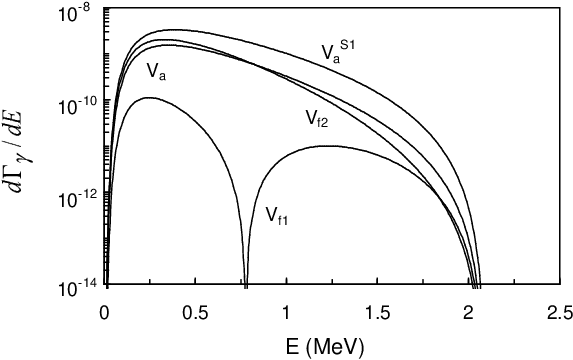
The integrated $\gamma$ widths (from $E=0$ up to $Q=2.089$ MeV) are given in Table 3 for the different potentials. The Gaussian potential $V_{a}$ simultaneously reproduces both the ⁶Li ground state binding energy and the $S$-wave phase shift at low energies. Additionally, the $S$-wave scattering wave function of this potential has two nodes at short distances (one due to the ground state, and one due to the Pauli forbidden state). The nearly phase-equivalent potential $V_{f2}$, which also has a forbidden bound state (and hence two nodes at short distances) gives similar results.

The influence of the nodes in the scattering wave function can be tested by using potential $V^{S1}_{a}$. The non-physical ground state of $V_{a}$ is removed by using a supersymmetric transformation [14]. The resulting phase-equivalent potential $V^{S1}_{a}$ has exactly the same ⁶Li ground-state energy and the same $S$-wave phase shift as $V_{a}$ but its scattering wave functions have one node less at small distances. The corresponding width of the M1 transition is about two times larger (see Table 3). In the ⁶He $\beta$-decay process, this potential strongly overestimates the data [4]. Notice that a very different result is obtained with the folding potential $V_{f1}$, which has two bound states, but does not reproduce the $\alpha+d$ phase shifts and the ⁶He delayed $\beta$ decay. The shape and magnitude of the transition width and probability are strongly different from the result for $V_{a}$.

Considering the $V_{a}$ and $V_{f2}$ potentials, which are consistent with the data on ⁶He $\beta$ decay, we deduce a recommended branching ratio of $1.3\times 10^{-4}$ by averaging both values. A previous estimate [2] of the branching ratio $\Gamma_{\gamma}(0^{+}\rightarrow\alpha+d)/\Gamma_{\gamma}(0^{+}\rightarrow 1^{+})$ provides $0.8\times 10^{-4}$. This value is close to our results obtained with potential $V_{a}$ [13], and is also similar to the branching ratio observed in the $\beta$ decay of ⁶He [17]. Such a branching ratio should be observable experimentally.

References

- [1] A. Csótó, K. Langanke, Nucl. Phys. A 601 (1996) 131.
- [2] L.V. Grigorenko, N.B. Shulgina, Phys. Atom. Nucl. 61 (1998) 1472.
- [3] Y. Suzuki, K. Yabana, Phys. Lett. B 272 (1991) 173.
- [4] E.M. Tursunov, D. Baye, P. Descouvemont, Phys. Rev. C 73 (2006) 014303; Phys. Rev. C 74 (2006) 069904(E).
- [5] M.V. Zhukov, B.V. Danilin, D.V. Fedorov, J.M. Bang, I.J. Thompson, J.S. Vaagen, Phys. Rep. 231 (1993) 151.
- [6] P. Descouvemont, C. Daniel, D. Baye, Phys. Rev. C 67 (2003) 044309.
- [7] V.I. Kukulin, V.N. Pomerantsev, Ann. Phys. NY 111 (1978) 330.
- [8] D.R. Thompson, M. LeMere, Y.C. Tang, Nucl. Phys. A 286 (1977) 53.
- [9] V.T. Voronchev, V.I. Kukulin, V.N. Pomerantsev, G.G. Ryzhikh, Few-Body Syst. 18 (1995) 191.
- [10] I. Tanihata, T. Kobayashi, O. Yamakawa, S. Shimoura, K. Ekuni, K. Sugimoto, N. Takahashi, T. Shimoda, H. Sato, Phys. Lett. 206B (1988) 592.
- [11] M. Puchalski, A.M. Moro, K. Pachucki, Phys. Rev. Lett. 97 (2006) 133001.
- [12] K. Arai, Y. Suzuki, K. Varga, Phys. Rev. C 51 (1995) 2488.
- [13] S.B. Dubovichenko, A.V. Dzhazairov-Kakhramanov, Phys. Atom. Nucl. 57 (1994) 733.
- [14] D. Baye, Phys. Rev. Lett. 58 (1987) 2738.
- [15] D.R. Tilley, C.M. Cheves, J.L. Godwin, G.M. Hale, H.M. Hofmann, J.H. Kelley, C.G. Sheu, H.R. Weller, Nucl. Phys. A 708 (2002) 3.
- [16] V.I. Kukulin, V.N. Pomerantsev, Kh.D. Razikov, V.T. Voronchev, G.G. Ryzhikh, Nucl. Phys. A 586 (1995) 151.
- [17] D. Anthony, L. Buchmann, P. Bergbusch, J.M. D’Auria, M. Dombsky, U. Giesen, K.P. Jackson, J.D. King, J. Powell, F.C. Barker, Phys. Rev. C 65 (2002) 034310.
- [18] L.S. Rodberg, R.M. Thaler, Introduction to the quantum theory of scattering, Academic Press (New York, 1967).
- [19] H.J. Rose, D.M. Brink, Rev. Mod. Phys. 393 (1967) 306.
- [20] D. Baye, P. Descouvemont, Nucl. Phys. A 443 (1985) 302.