Final state radiation and a possibility to test a pion-photon interaction model near two-pion threshold.

The ongoing experiments on precise measurements of the cross section of $e^{+}e^{-}$ annihilation into hadrons aim to a precision at the $0.5-1.0\%$ level [1, 2, 3]. Such an accuracy is crucial for various tests of the Standard Model [4], e.g., by confronting the experimentally measured value of $a_{\mu}$ [5], the muon anomalous magnetic moment, to the theoretical prediction. The accuracy of the theoretical calculation of $a_{\mu}$ is currently limited by the hadronic contribution, $a_{\mu}^{(had)}$. This contribution cannot be reliably calculated in the framework of perturbative QCD, because low-energy region dominates. Fortunately, its leading order part, $a_{\mu}^{(had;LO)}$, can be estimated from the dispersion relation using the experimental cross sections of $e^{+}e^{-}$ annihilation as an input [4]

where $\sigma_{h}(q^{2})$ is the total hadronic cross section, $\sigma_{\mu}(q^{2})$ is the total cross section of the process $e^{+}e^{-}\to\gamma\to\mu^{+}\mu^{-}$ and the function $K(q^{2})$ is a smooth function that increases from $0.63$ at the threshold ($s=4m_{\pi}^{2}$) upto $1$ for $q^{2}\to\infty$. The quantity $q^{2}$ is the total four momentum squared of the final hadrons.

This behaviour of the integrand results in that the biggest contribution (about $70\%$) to the leading order hadronic part of the muon anomalous magnetic moment, $a_{\mu}^{(had;LO)}$, comes from the energy region below or about $1$ GeV. Due to the presence of the $\rho$-meson the main contribution is related with the $\pi^{+}\pi^{-}$ final state.

Experimentally, the energy region from threshold to the collider beam energy is explored at the $\Phi$-factory DA$\Phi$NE (Frascati, $s=4E^{2}=m_{\phi}^{2}$) [6, 7] and B-factory, PEP-2 (SLAC, $s=m_{\Upsilon(4S)}^{2}$) and KEKB (KEK, $s=m_{\Upsilon(4S)}^{2}$) [8, 9] using the method of radiative return [10, 11, 12]. This method relies on a factorization of the radiative cross section in the product of the hadronic cross section and a radiation function $H(q^{2},\theta_{max},\theta_{min})$ known from Quantum Electrodynamics (QED) [12, 13, 14]. The large luminosity of the $\Phi$ and $B$-factories allows to compensate the additional factor $\displaystyle\frac{\mathstrut\alpha}{2\pi}$ caused by the hard photon emission.

For a two-pion final state considered here it means that the radiative cross section $\sigma^{\pi\pi\gamma}$ corresponding to the process

can be written as

where the hadronic cross section $\sigma^{\pi\pi}$ is taken at a reduced CM energy. This factorization is valid only for photon radiation from the initial leptons (initial state radiation (ISR)). This is not possible for final state (FS) radiation (FSR) which is an irreducible background in radiative return measurements of the hadronic cross section [2, 15]. ¹¹ 1 In fact the process of FSR cannot be excluded from the analysis. It can be suppressed choosing the small angle kinematics ($\theta_{\gamma}<\theta_{max}\ll 1$) but for the large angle analysis this contribution becomes upto $40\%$ of ISR and should be estimated very carefully. (For some advantages of large angle analysis compared to small angle one see [16].) Indeed, the FSR cross section calculation has an additional complication compared to ISR case. In principle, RC caused by initial state radiation, i.e. the function $H(q^{2},\theta_{max},\theta_{min})$, can be calculated in QED, although the accuracy is technically limited. Instead, for the calculation of the FSR cross section the situation is different since its evaluation relies on models describing pion–photon interaction. Usually the combined sQED$*$VMD model is assumed as a model to calculate FS Bremsstrahlung process [12, 17]. In this case the pions are treated as point-like particles (the sQED model) and the total FSR amplitude is multiplied by the pion form factor, that is estimated in the VMD model. Unfortunately, the sQED$*$VMD model is an approximation that is valid for relatively soft photons and it can fail for high energy photons, i.e near the $\pi^{+}\pi^{-}$ threshold. In this energy region the contributions to FSR, beyond the sQED$*$VMD model, can become important. As it was shown in Ref. [18] the Resonance Perturbation Theory (RPT) is an appropriate model to describe photon-meson interactions in the energy region about $1$ GeV and we will apply this model to estimate the Bremmstrahlung FS contributions beyond of sQED.

At thet $\Phi$ factory DA$\Phi$NE there is an additional complication related with the possible intermediate $\phi$ meson state and the corresponding contributions should be included in the Monte Carlo event generator.

In this paper we present the results obtained by the Monte Carlo event generator FEVA that simulates the process (2) for the DA$\Phi$NE accelerator setup. Our computer code FEVA was inspired by MC EVA [12]. The previous version of FEVA was described in [19], where the Bremsstrahlung process (both in the framework of RPT and sQED) and the $\phi$ direct decay (only $f_{0}$ parameterization) were considered. The current version of FEVA includes in addition the double resonance contribution and a more sophisticated parameterization for the $\phi$ direct decay.

This paper is organized as follows. In Section 2 we give a general description of FSR process and present the FSR models that have been already included in our program FEVA. In Section 3 the numerical results for the KLOE large angle analysis are presented. Since most of the effects arising in the FSR are model-dependent, we conclude this paper by suggesting a way to test possible effects beyond sQED, in a model-independent way (see Section 4). A conclusion is given in Section 5.

The cross section of the FSR process can be written as

where $Q=p_{1}+p_{2}$, $s=Q^{2}$,

and where the FS tensor $M^{\mu\nu}$ describes the transition

It is convenient to parametrize the FS tensor in terms of three gauge invariant tensors (see [20] and Ref. $[23,24]$ in it):

We would like to emphasize that this expansion is totally model-independent. The model dependence is related only with an explicit form of the scalar functions $f_{i}$ (we will call them structure functions).

Here is the list of the FSR processes included in FEVA MC:

In the next sections we present the models describing these processes. The presence of (8) and (9) is due to the energy at which KLOE is running($s=m_{\phi}^{2}$).

In this chapter we present the results for the differential cross section and the forward-backward asymmetry [12, 29] for the reaction $e^{+}e^{-}\to\pi^{+}\pi^{-}\gamma$, where the FSR amplitude ($M_{FSR}$) receives contributions from both RPT ($M_{RPT}$) and the $\phi\to\pi^{+}\pi^{-}\gamma$ decay ($M_{\phi}$). The last one is a sum of the $\phi$ direct decay ($M_{\phi}^{scal}$) and VMD ($M_{\phi}^{VMD}$) contributions. Thus the total contribution of the process (2) $d\sigma_{T}$ can be written as:

where $d\sigma_{I}$ corresponds to the ISR cross section, $d\sigma_{F}$ is for the FSR one. The interference term $d\sigma_{IF}$ is equal to zero for symmetric cuts on the polar angle of the pions [7].

The different contributions to the FSR differential cross section $d\sigma_{F}$, evaluated at $s=m_{\phi}^{2}$, are shown in Fig.1, right, for the full angular range $0^{\circ}\leq\theta_{\gamma}\leq 180^{\circ},0^{\circ}\leq\theta_{\pi}\leq 180^{\circ}$. Good agreement between the results of the Monte Carlo simulation (points), with the analytic prediction (solid line) is found. It can be noted that at low $Q^{2}$ the contribution from the direct $\phi$ decay (i.e. the term proportional to $|M_{\phi}^{scal}|^{2}$ in Eq. (32)) is quite large and, therefore, the additional contribution beyond sQED, can be revealed only in the case of destructive interference between the two amplitudes ($\mathrm{Re}(M_{RPT}\cdot M_{\phi}^{*})<0$). Published data from the KLOE experiment [2] are in favour of this assumption, which we will use in the following.

To begin with, we consider the case $s=m_{\phi}^{2}$. In Fig.2 we show the values of the differential cross section $d\sigma_{T}/d\sigma_{I}$ and the forward-backward asymetry for the angular cuts of the KLOE large angle analysis [16, 30]:

for the Bremsstrahlung FS process in the framework of the sQED$*$VMD model and with the $\phi$ decay contributions (VMD and the $\phi$ direct decay), for a hard photon radiation with energies $E_{\gamma}>20$ MeV.

Figure 3 shows the effects of RPT and $\phi$ direct decay terms to the total differential cross section and their contribution to FSR one for angular cuts (3). Several distinctive features can be noted:(1) the peak at about $1$ GeV² corresponds to the $f_{0}$ intermediate state for the direct $\phi\to\pi\pi\gamma$ amplitude; (2) the presence of RPT terms in the FSR is relevant at low $Q^{2}$, where they give an additional contribution up to $40\%$ to the ratio $d\sigma_{RPT+\phi}/d\sigma_{sQED+\phi}$; (as shown in Fig. 3,left); (3) the destructive interference between the $\phi$ decay an the Bremsstrahlung FS process decreases the visible cross section in the whole $Q^{2}$ region and its dependence on FS Bremsstrahlung model at low $Q^{2}$ (see Fig. 2, left, down). Also we would like to draw attention to the VMD contribution. As we can see from Fig. 2, the VMD contribution almost does not change the value of the differential cross section (Fig. 2, left), but it changes essentially the value of the forward-backward asymmetry (Fig. 2, right) and it follows the experimental data for it. Last but not least, all contributions beyond sQED are large enough near the threshold to make the analysis difficult.

In order to reduce the background from $\phi$ decay in the measurement of the pion form factor at threshold, KLOE has taken more than $200$ pb^-1 of data at 1 GeV [31]. In this case the $\phi$ meson intermediate contributions are suppressed (see Fig. 4, (right), the values of $d\sigma_{T}$ with and without the $\phi$ decay almost coincide) and the main contribution to FSR comes from Bremsstrahlung process (see Section 2.1), allowing to study a model for it.

Contributions to Bremsstrahlung FS process beyond sQED, as in the case of RPT, can lead to sizeable effects on the cross section and asymmetry at threshold, as shown in Figs. 2-4. Precise measurement of the pion form factor in this region needs to control them at the required level of accuracy. This looks like a rather difficult task, if one thinks that effects beyond sQED, as well as the contribution from $\phi\to\pi^{+}\pi^{-}\gamma$, are model-dependent.

One can think to construct a general amplitude for the $e^{+}e^{-}\to\pi^{+}\pi^{-}\gamma$, according to some underlying theory, and try to determine the free parameters by a constrained fit on specific variables (like mass spectrum, charge and forward-backward asymmetry, angular distribution, etc…). Particularly for the charge asymmetry, it has been proved to be a powerful tool to discriminate between different models of $\phi\to\pi^{+}\pi^{-}\gamma$ [29]. However, when the number of the parameters is large, correlations between the parameters of the model can arise and spoil the effective power of these fits. The situation becomes even worse if the pion form factor also has to be extracted from the same data. As an example, in the case of RPT model, if we consider only the $\rho$ and $\omega$ contribution to the pion form factor and the $\rho$ and $a_{1}$ contribution to FSR the number of free parameters is already six. The presence of the $\phi$ direct and VMD decays results in additional free parameters.

The possibility to determine some of the parameters by external data can strongly help, as in the case of the $\phi\to\pi^{+}\pi^{-}\gamma$ amplitude, which can be determined by the $\pi^{0}\pi^{0}\gamma$ channel copiously produced at DA$\Phi$NE. An additional source of information, which will be used to determine the contributions to FSR beyond sQED in a model-dependent way, is the dependence of the FSR amplitude on the $e^{+}e^{-}$ invariant mass squared $s$.

Let us write the differential cross section for the emission of one photon in the process $e^{+}e^{-}\to\pi^{+}\pi^{-}\gamma$ as a function of the invariant mass of the two pions:

where $\Big(\mathstrut\frac{\displaystyle d\sigma_{F}}{dQ^{2}}\Big)_{s}$ is the differential cross section for the emission of a photon in the final state, while the ISR function $H_{s}(Q^{2})$ was defined in the Introduction. We indicate by a subscript $s$ the dependence of each quantity on the $e^{+}e^{-}$ invariant mass ($s$). Since we will consider only symmetric angular cuts for pions, the interference term between initial and final state radiation has been neglected.

At relatively high $Q^{2}$ the FSR differential cross section, $\Big(\mathstrut\frac{\displaystyle d\sigma_{F}}{dQ^{2}}\Big)_{s}$, is dominated by the contribution coming from sQED ($M_{sQED}$) and $\phi$ direct decay ($M_{\phi}$):

Contributions beyond sQED ($\Delta M$) are expected to be important at low $Q^{2}$. They introduce an additional term ($\Delta M$) in the above expression:

We will now consider the following quantity:

where $\Delta F_{s}\sim\Big(|\Delta M|^{2}+2\mathrm{Re}\Big\{\Delta M\cdot(M_{sQED}+M_{\phi})^{*}\Big\}\Big)_{s}/H_{s}$.

If no contribution beyond sQED is present ($\Delta M=0$), $Y_{s}(Q^{2})$ coincides with the square of the pion form factor, independently of the energy $\sqrt{s}$ at which it is evaluated, while any dependence on $s$ is only due to an additional contribution to FSR beyond sQED. In particular, the difference of $Y_{s}(Q^{2})$ computed at two beam energies ($s_{1}$ and $s_{2}$), can only come from FSR beyond sQED:

Therefore, before extracting the pion form factor at threshold, we suggest to look at the difference $\Delta Y(Q^{2})$, which can be used to estimate the contribution beyond sQED to the FSR amplitude in a model-independent way.

As a realistic application of this procedure, we consider the case of DA$\Phi$NE, where KLOE has already collected more than 200 pb^-1 at 1 GeV² and 2.5 fb^-1 at $m_{\phi}^{2}$, that, in the range $Q^{2}<0.35$ GeV² , correspond to $O(10^{3})$ and $O(10^{4})$ events, respectively, in the region $50^{\circ}\leq\theta_{\gamma}\leq 130^{\circ}$, $50^{\circ}\leq\theta_{\pi}\leq 130^{\circ}$. We will consider RPT as a model for the effects beyond sQED.

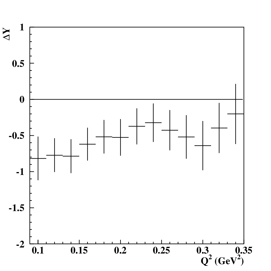
Fig. 5, left, shows the quantity $Y_{s}(Q^{2})$ at $s_{1}=1$ GeV² and at $s_{2}=m_{\phi}^{2}$ when no additional RPT term is included in FSR. As expected, each of these quantities coincides with the square of the pion form factor $|F_{\pi}(Q^{2})|^{2}$, shown by a solid line. The difference $\Delta Y(Q^{2})$ is shown in Fig.5, right, which is consistent with zero as expected. In the region $s<0.35$ GeV² one can expand the pion form factor as it was done in [4]:

Using the same experimental data for the pion form factor [1] as before we have: $p_{1}=1.15\pm 0.06$ GeV^-2, $p_{2}=9.06\pm 0.25$ GeV^-4, $\chi^{2}/\nu\simeq 0.13$. A combined fit of $Y_{s}(Q^{2})$ to the pion form factor gives the following values: $p_{1}=1.4\pm 0.186$ GeV^-2, $p_{2}=8.8\pm 0.73$ GeV^-4, $\chi^{2}/\nu=0.25$, that is in a reasonable agreement with the results (40).

The situation is different as soon as the Bremsstrahlung FS process is modeled by RPT. In this case, as shown in Fig.6, right, the difference $\Delta Y(Q^{2})\neq 0$ and the quantities $Y_{s}(Q^{2})$ cannot be anymore identified with $|F_{\pi}(Q^{2})|^{2}$, (see Fig.6, left) ⁶⁶ 6 Destructive interference between RPT and $\phi\to\pi^{+}\pi^{-}\gamma$ amplitudes tends to cancel out the effects beyond sQED at $s=m_{\phi}^{2}$ (see Fig. 3, left). Therefore the quantity $Y_{s}(Q^{2})$ almost coincides with the pion form factor..

Before concluding, we would like to point out the main points of our present method:

• •

  The quantity $\Big(\frac{d\sigma_{sQED+\phi}}{dQ^{2}}\Big)_{s}$ is an input parameter of our procedure, and can be computed numerically by Monte Carlo;

• •

  The amplitude for $\phi\to\pi^{+}\pi^{-}\gamma$ is taken from the $\pi^{0}\pi^{0}\gamma$ channel.

• •

  missing ISR multi-photon radiative correction can be added in $H_{s}$ and it will not spoil the effective power of the method;

• •

  A clear advantage of the procedure based on a Monte Carlo event generator is that it allows to keep control over efficiency and resolution of the detector and fine tuning of the parameters.

Even if the main limitation of the method could come from the uncertainty on the parameters of $\phi\to\pi^{+}\pi^{-}\gamma$ amplitude, especially at low $Q^{2}$, we believe that the KLOE data on $\phi\to\pi^{0}\pi^{0}\gamma$ will allow a precise description of this amplitude. In any case, in agreement with [29] we strongly recommend to check the amplitude by using charge asymmetry and to compare with spectrum of the $\pi^{+}\pi^{-}\gamma$, at least at high $Q^{2}$, where the pointlike approximation is safe (as done in [30]).

A test of FSR at threshold in the process $e^{+}e^{-}\to\pi^{+}\pi^{-}\gamma$ is a rather important issue, not only for the role of FSR as background to the measurement of the pion form factor, but also to get information about pion-photon interactions when the intermediate hadrons are far off shell. At $s=m_{\phi}^{2}$ an additional complication arises: the presence of the decay $\phi\to\pi^{+}\pi^{-}\gamma$, that goes either through the intermediate scalar (the direct $\phi$ decay) or the vector state (VMD contribution) whose amplitude and relative phase can be described according to some model. By means of a Monte Carlo event generator FEVA, which also includes the contribution of the rare $\phi\to\pi^{+}\pi^{-}\gamma$ decay, we estimate the effects beyond sQED in the framework of Resonance Perturbation Theory (RPT) for angular cuts used in the KLOE analysis of the pion form factor at threshold. We show that the low $Q^{2}$ region is sensitive both to the inclusion of additional terms in the FSR amplitude given by the RPT model and to the $\phi$ decay contribution (especially its VMD part).

References

- [1] R.R. Akhmetshin, V.M. Aulchenko, V. Banzarov et al. [CMD-2 Collaboration], Phys. Lett. B 648, 28 (2007).
- [2] A. Aloisio, F. Ambrosino, A. Antonelli et al. [KLOE Collaboration], Phys. Lett. B 606, 12 (2005).
- [3] M.N. Achasov, K.I. Beloborodov, A.V. Berdyugin it et al. [SND Collaboration], J. Exp. Theor. Phys 103, 380 (2006).
- [4] S. Eidelman and F. Jegerlehner, Z. Phys. C 67, 585 (1995).
- [5] G.W. Bennett, B. Bousquet, H.N. Brown et al., Phys. Rev. D 73, 072003 (2006).
- [6]
G. Cataldi, A.G. Denig, W. Kluge, S. Müller and G. Venanzoni,
in Frascati 1999, Physics and detectors for DANE,
p. 569;
A. Aloisio, F. Ambrosino, A. Antonelli et al., The KLOE Collaboration, hep-ex/0107023. - [7]
S. Spagnolo, Eur. Phys. J. C 6, 637 (1999);
A. Aloisio, F. Ambrosino, A. Antonelli et al., The KLOE Collaboration, hep-ex/0312056. - [8]
E.P. Solodov, The BaBar Collaboration, hep-ex/0107027;
G.Sciolla, The BABAR Collaboration, Nucl. Phys. B (Proc. Suppl.) 99, 135 (2001).
N. Berger, hep-ex/0209062; - [9] M. Benayoun, S.I. Eidelman, V.N. Ivanchenko and Z.K. Silagadze, Mod. Phys. Lett. A 14, 2605 (1999).
- [10] Min-Shin Chen and P.M. Zerwas, Phys. Rev. D 11, 58 (1975).
- [11]
A.B. Arbuzov, E.A. Kuraev, N.P. Merenkov and L. Trentadue, JHEP
12, 009 (1998);
M. Konchatnij and N.P. Merenkov, JETP Lett. 69, 811 (1999). - [12]
S. Binner, J. H. Kühn and K. Melnikov,
Phys. Lett. B 459, 279 (1999);
J. Kühn, Nucl. Phys. B (Proc. Suppl.) 98, 2 (2001). - [13] V.N. Baier and V.A. Khoze, Sov. Phys. JETP 21, 629 (1965); ibid., 21, 1145 (1965).
- [14] V.A. Khoze, M.I. Konchatnij, N.P. Merenkov et al., Eur. Phys. J. C 25, 199 (2002).
- [15] H. Czyż, A. Grzelińska, J. H. Kühn and G. Rodrigo, Eur. Phys. J. C 33,333 (2004).
- [16] D. Leone, Nucl. Phys. B - Proc. Suppl. 162, 95 (2006).
- [17] H. Czyż, A. Grzelinska, J. H. Kühn and G. Rodrigo, Eur. Phys. J. C 27, 563 (2003).
- [18]
G. Ecker, J. Gasser, A. Pich and E. de Rafael, Nucl.
Phys. B 321, 311 (1989);
G. Ecker, J. Gasser, H. Leutwyler, A. Pich and E. de Rafael, Phys. Lett. B 223, 425 (1989). - [19] G. Pancheri, O. Shekhovtsova, G. Venanzoni, Phys. Lett. B 642, 342 (2006).
- [20] S. Dubinsky, A. Korchin, N. Merenkov, G. Pancheri and O. Shekhovtsova, Eur. Phys. J. C 40, 41 (2005).
- [21] S. Eidelman, K.G. Hayes, K.A. Olive et al. [Particle Data Group], Phys. Lett. B 592, 1 (2004).
- [22] K. Melnikov, F. Nguyen, B. Valeriani and G. Venanzoni, Phys. Lett. B 477, 114 (2000).
- [23] G. Isidori, L. Maiani, M. Nicolaci and S. Pacetti, JHEP 0605:049, 2006.
- [24] N. N. Achasov, V. V. Gubin and E. P. Solodov, Phys. Rev. D 55, 2672 (1997).
- [25] F. E. Close, N. Isgur and S. Kumano, Nucl. Phys. B 389, 513 (1993). J. L. Lucio Martinez and M. Napsuciale, Phys. Lett. B 331, 418 (1994).
- [26] A. Aloisio,F. Ambrosino, A. Antonelli it et al. [KLOE Collaboratio], Phys. Lett. B 537, 21 (2002).
- [27] N.N. Achasov and A.V. Kiselev, Phys. Rev. D 73, 054029 (2006).
- [28] F. Ambrosino, A. Antonelli, M. Antonelli et al. [KLOE Collaboration], Eur. Phys. J. C 49, 473 (2007).
- [29] H. Czyż, A. Grzelinska and J. H. Kühn, Phys. Lett. B 611, 116 (2005).
- [30] F. Ambrosino, A. Antonelli, M. Antonelli et al. [KLOE Collaboration], Phys. Lett. B 634, 148 (2006).
- [31]
A. Denig, Nucl. Phys. B - Proc. Suppl. 162, 81 (2006);
S. Müller, PhD thesis (www-ekp.physik.uni-karlsruhe.de/pub/web). - [32]
R.M. Carey et al., Proposal of the BNL Experiment E969, 2004 (www.bnl.gov/henp/docs/pac0904/P969.pdf);
B.I. Roberts, hep-ex/0501012. - [33] ’Working Group on Radiative Corrections and MC Generators for Low Energies’, http://www.lnf.infn.it/wg/sighad.