Water-like hierarchy of anomalies in a continuous spherical shouldered potentialPreprint: PREPRINT

Alan Barros de Oliveira Affiliation: Instituto de Física, Universidade Federal do Rio Grande do Sul, Caixa Postal 15051, 91501-970, Porto Alegre, Rio Grande do Sul, Brazil. Email: oliveira@if.ufrgs.br Giancarlo Franzese Affiliation: Departament de Física Fonamental, Facultat de Física, Universitat de Barcelona, Diagonal 647, 08028, Barcelona, Spain. Email: gfranzese@ub.edu Paulo A. Netz Affiliation: Instituto de Química, Universidade Federal do Rio Grande do Sul, 91501-970, Porto Alegre, Rio Grande do Sul, Brazil. Email: netz@iq.ufrgs.br Marcia C. Barbosa Affiliation: Instituto de Física, Universidade Federal do Rio Grande do Sul, Caixa Postal 15051, 91501-970, Porto Alegre, Rio Grande do Sul, Brazil . Email: marcia.barbosa@ufrgs.br

December, 8 2007

Abstract

We investigate by molecular dynamics simulations a continuous isotropic core-softened potential with attractive well in three dimensions, introduced by Franzese [J. Mol. Liq. 136, 267 (2007)], that displays liquid-liquid coexistence with a critical point and water-like density anomaly. Besides the thermodynamic anomalies, here we find diffusion and structural anomalies. The anomalies, not observed in the discrete version of this model, occur with the same hierarchy that characterizes water. We discuss the differences in the anomalous behavior of the continuous and the discrete model in the framework of the excess entropy, calculated within the pair correlation approximation.

pacs

64.70.Pf, 82.70.Dd, 83.10.Rs, 61.20.Ja

I Introduction

Experiments for water allow to locate the line of temperatures of maximum density (TMD) below which the density decreases with decreasing temperature at constant pressure, instead of increasing as in the majority of fluids. An76 Experiments for Te, Th76 Ga, Bi, LosAlamos S, Sa67; Ke83 and Ge₁₅Te₈₅, Ts91 and simulations for silica, An00; Ru06b; Sh02; Po97 silicon Sa03 and BeF₂, An00 show, as well, the same density anomaly.

Water also has dynamic anomalies. Experiments for water show that the diffusion constant, $D$ , increases on compression at low temperature $T$ up to a maximum $D_{\rm max}(T)$ at $P=P_{D\mathrm{max}}(T)$ . The behavior of normal liquids, with $D$ decreasing on compression, is restored in water only at high $P$ , e.g. for $P>P_{D\mathrm{max}}\approx 1.1$ kbar at 10 ^oC. An76 Numerical simulations for SPC/E water spce recover the experimental results and show that the anomalous behavior of $D$ extends to the metastable liquid phase of water at negative pressure, a region that is difficult to access for experiments. Ne01; Er01; Mi06a; Ku06 In this region the diffusivity $D$ decreases for decreasing $P$ until it reaches a minimum value $D_{\rm min}(T)$ at some pressure $P_{D\mathrm{min}}(T)$ , and the normal behavior, with $D$ increasing for decreasing $P$ , is reestablished only for $P<P_{D\mathrm{min}}(T)$ . Ne01; Er01; Mi06a; Mu05

In order to shade some light in the relation between the thermodynamic and dynamic anomalies, Errington and Debenedetti investigated the pressure-dependence of the structure of SPC/E water by measuring (i) the tendency of pairs of molecules to adopt preferential separations, by means of a translational order parameter, and (ii) the extend to which a molecule and its four nearest neighbors assume a tetrahedral arrangement, by means of an orientational order parameter. Er01 They found a region of the $P$ - $T$ phase diagram, called the structural anomalous region, where both order parameters decrease for increasing density, i.e. the liquid is more disordered at higher density, in contrast with the behavior of normal liquids. They showed that the structural anomalous region encompasses the region where the diffusion is anomalous, and that the latter includes the region where the density is anomalous. Next, Shell, Debenedetti, and Panagiotopoulos used the two structural order parameters to study the case of a computer model for silica. Both order parameters demonstrated to be anomalous, but the hierarchy of anomalies for silica is different compared to water. Sh02 For silica the diffusion anomalous region is the wider one, containing the structural anomalous region which in turn has inside the density anomaly region.

The study of core-softened potentials generates models that are computationally (sometimes even analytically) tractable and that may retain some qualitative features of network forming fluids such as water and silica. What they have in common with the water potential is the two interaction scales that in the case of water are the van der Waals and the hydrogen bond interaction distances. In some cases, theoretical Xu06; Ol05; Ol06a; Ol06b; Wi06; Ya05; Ya06; Fr07a and experimental Sh07 results for core-softened potentials show the presence of anomalies. In other cases, in particular for the discontinuous shouldered well (DSW) potential, no density anomaly is observed. Fr01; Fr02; Sk04; Ma05 The DSW potential consists of a hard core, a square repulsive shoulder and an attractive square well (dashed line in Fig. 1).

In this paper, we investigate the presence of water-like anomalies in a continuous shouldered well (CSW) potential introduced by Franzese Fr07a (continuous line in Fig. 1). Although the model is similar to the DSW version, we find density, diffusion, and structural anomalies and we observe that they occur with the same hierarchy as in water. In order to get a better understanding of the reasons why the CSW potential displays water-like anomalies, while the DSW one does not, we apply recent ideas that have emerged on the connection between the anomalies and the excess entropy.Ru06b; Mi06a; Mi06b

Since the model studied here resembles effective potentials for complex liquids or liquid metals, our results suggest that the water-like hierarchy of anomalies could be experimentally found in systems where pressure-induced bond shortening, rather than the change in the coordination number, is the origin of the density anomaly. Sh07

The outline of the paper is as follows. We present the details of the model in Sec. II, and the details of the simulations in Sec. III. In Sec. IV we show and discuss the results obtained from simulations and in Sec. V we summarize and give the conclusions.

II The model

The CSW model Fr07a studied here is composed by a system of identical particles interacting through the potential (Fig. 1) defined as

U(r)=\frac{U_{R}}{1+\exp\left[\Delta\left(r-R_{R}\right)/a\right]}-U_{A}\exp\left[-\frac{(r-R_{A})^{2}}{2\delta_{A}^{2}}\right]+\left(\frac{a}{r}\right)^{24},

(1)

where $U_{R}$ and $U_{A}$ are the energy of the repulsive shoulder and of the attractive well, respectively, $a$ is the diameter of particles, $R_{R}$ and $R_{A}$ are the repulsive average radius and the distance of the attractive minimum, respectively, $\Delta$ is a parameter related to the slope of the potential at $R_{R}$ ; $\delta_{A}^{2}$ is the variance of the Gaussian centered at $R_{A}$ . The many parameters of this potential allow it to assume several forms, similar to the potential proposed by Cho, Ch96a ranging from a deep double wells Ch96a; Ch97a; Ne04 to repulsive ramp-like potentials, Ol06a; Ol06b; Ol07 making this equation malleable for studying different isotropic models for systems such as colloids or liquid metals. Details about the role played by these parameters may be found in Ref. Fr07a. The set of parameters used here is the same as in Ref. Fr07a: $U_{R}/U_{A}=2,$ $\Delta=15,$ $R_{R}/a=1.6,$ $R_{A}/a=2,$ $(\delta_{A}/a)^{2}=0.1,$ with cutoff $r_{c}=3.0a$ . To have a continuous function at the cutoff distance, a constant $C/U_{A}=0.208876$ and a linear term $\lambda r/a$ , with $\lambda/a=-0.0673794$ , are added. Fr07a The CSW potential may be interpreted as a continuous version of the DSW potential investigated in Refs. Fr01; Fr02; Ba04; Sk04; Ma05. The corresponding DSW potential is represented by a square shoulder of size $\mathrm{w_{R}}/a$ and a well of size $\mathrm{w_{A}}/a$ and depth $\mathrm{U_{R}}+\mathrm{U_{A}}$ illustrated by the dashed line in in Fig. 1 (the parameters in figure are $\mathrm{w_{R}}/a=0.612$ , $\mathrm{w_{A}}/a=0.767$ , $\mathrm{U_{R}}/\mathrm{U_{A}}=2.2$ ).

III Details of simulations

In order to investigate the interparticle CSW potential Eq. (1), we employ a molecular dynamics (MD) technique. Frenkel We consider 1000 particles in a cubic box with periodic boundary condition. We perform simulations in the NVT ensemble with the Nosé-Hoover thermostat Frenkel and coupling parameter equal to 2. Pressure, temperature, density, and diffusion are calculated in dimensionless units, $P^{*}\equiv Pa^{3}/U_{A}$ , $T^{*}\equiv k_{B}T/U_{A}$ , $\rho^{*}\equiv\rho a^{3}$ , and $D^{*}\equiv D\left(m/a^{2}U_{A}\right)^{1/2}$ .

Positions, velocities, and configurational energy of the particles are stored for every $100$ steps, during a total time of $10^{6}$ steps, given a total of $10^{4}$ stored configurations. Pressure, diffusion, and order parameters are calculated over these configurations, discarding the first $2\times 10^{3}$ for equilibration purposes. The time step used is $2\times 10^{-3}$ in units of $(a^{2}m/U_{A})^{1/2}$ (of the order of $\approx 1.3\times 10^{-12}$ s for argon-like atoms and $\approx 1.1\times 10^{-12}$ s for water-like molecules).

The model displays Fr07a a phase diagram with two first-order phase transitions ending in critical points: one transition between gas and low-density liquid (LDL) phases and another between LDL and high-density liquid (HDL) phase. The LDL-HDL phase transition is metastable with respect to the crystal phase.

For temperatures and densities inside the metastable region the positions, velocities, and configuration energy are stored for every 10 steps and the quantities are calculated with the configurations stored until the drop in configuration energy and virial, discarding the equilibration time. The time before the drop in energy and virial characterizes the lifetime of the metastable phase.

IV Results and discussion

IV.1 Density anomaly

In the vicinity of the LDL-HDL critical point the system shows density anomaly. Fr07a The isochores have a temperature of minimum pressure in the interval $0.185<\rho^{*}<0.215$ , corresponding to the temperature of maximum density (TMD) at constant $P$ [Fig. 2(a)]. Inside the TMD line the density decreases as the system is cooled at constant $P$ . For densities in the range $0.2<\rho^{*}<0.215$ , the TMD line is negatively sloped, while it has positive slope for $0.185<\rho^{*}<0.2$ . Our results for the TMD line in the ranges $0.55\leq T^{*}\leq 0.61$ and $0.25\leq P^{*}\leq 0.30$ [Fig. 2(d)] compares well, qualitatively, with the experimental data for water, An76 showing a negative slope [Fig. 2(b)]. The data in all the supercritical region [Fig. 2(a)] resemble the simulation results for SPC/E water, Ne01 with a retracing TMD line [Fig. 2(c)]. Nevertheless, in the present case the TMD line is at $P>0$ for all its length, while for SPC/E water it extends to negative pressures.

IV.2 Diffusion anomaly

The diffusion coefficient is calculated using the mean-square displacement averaged over different initial times,

\langle\Delta r(t)^{2}\rangle=\langle[r(t_{0}+t)-r(t_{0})]^{2}\rangle.

(2)

From Eq. (2), the diffusion coefficient may be obtained as follows:

D=\lim_{t\to\infty}\langle\Delta r(t)^{2}\rangle/6t.

(3)

While for normal fluids diffusivity decreases monotonically with increasing density at constant temperature, for the model Eq. (1) this is the case only for temperatures $T^{*}>0.64$ (Fig. 3). For $T^{*}<0.64$ , the diffusion coefficient has three regions: (i) For $\rho<\rho_{D\mathrm{min}}$ , $D$ decreases as $\rho$ increases as expected for normal fluids. (ii) For $\rho_{D\mathrm{min}}<\rho<\rho_{D\mathrm{max}}$ , $D$ increases with density – an anomalous behavior. This region is called the anomalous diffusion region. (iii) For $\rho>\rho_{D\mathrm{max}}$ , the normal behavior is restored with $D$ decreasing as density increases.

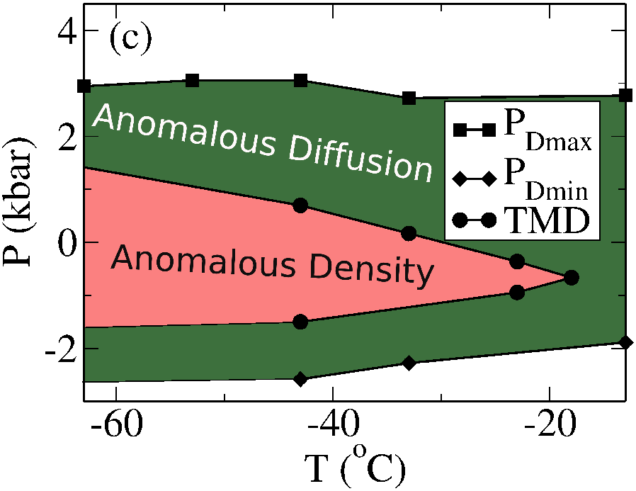
The line of $P_{D\mathrm{max}}(T)$ in the $P$ - $T$ phase diagram [Fig. 2(d)] is consistent with the diffusivity maxima observed in experiments for water [Fig. 2(b)]. Moreover, both lines of diffusion extrema, $P_{D\mathrm{max}}(T)$ and $P_{D\mathrm{min}}(T)$ [Fig. 2(a)], resemble the results for detailed models of water Ne01; Er01; Mi06a [Fig. 2(c)], silica, Po97; Ru06a; Sh02 and other isotropic potentials. Xu06; Ya05; Ya06; Ol06a We find that our $D_{\mathrm{min}}$ , like other isotropic models, Xu06; Ya05; Ya06; Ol06a occur at positive $P$ .

IV.3 Structural anomaly

The two quantities used for studying the structural behavior of the system of particles interacting through the potential in Eq. (1) are the translational order parameter, $t,$ and the orientational order parameter, $Q_{6}.$ The translational order parameter is defined as Er01; Sh02; Er03

t\equiv\int_{0}^{\xi_{c}}|g(\xi)-1|d\xi,

(4)

where $\xi\equiv r\rho^{1/3}$ is the distance $r$ in units of the mean interparticle separation $\rho^{-1/3}$ , $\xi_{c}$ is the cutoff distance set to half of the simulation box times $\rho^{-1/3}$ , as in Ref. Ol06b, $g(\xi)$ is the radial distribution function proportional to the probability of finding a particle at a (reduced) distance $\xi$ from a reference particle. For an ideal gas $g=1$ and $t=0$ . In the crystal phase $g\neq 1$ over long distances and $t$ is large.

For normal fluids, $t$ increases with increasing density. We find this monotonic behavior only for $T^{*}\geq 1.8$ (Fig. 4). For $T^{*}<1.8$ we observe that $t$ has a maximum at $\rho_{t\mathrm{max}}(T)$ , decreases for increasing $\rho>\rho_{t\mathrm{max}}(T)$ , reaches a minimum at $\rho_{t\mathrm{min}}(T)$ , and recovers the normal increasing behavior for $\rho>\rho_{t\mathrm{min}}(T)$ (Fig. 4).

For each particle $i=1,\dots,N$ we calculateEr01; Sh02; St83; Er03; To00; Tr00; Hu04

Q_{\ell}^{i}=\left[\frac{4\pi}{2\ell+1}\sum_{m=-\ell}^{m=\ell}\left|\overline{\left(Y_{\ell m}^{i}\right)}_{k}\right|^{2}\right]^{1/2},

(5)

with $\ell=6$ . The quantity $\overline{\left(Y_{\ell m}^{i}\right)}_{k}={1\over k}\sum_{j=1}^{k}Y_{\ell m}(\theta_{ij},\phi_{ij})$ is the average over the spherical harmonics $Y_{\ell m}$ calculated over the vectors ${\bf r}_{ij}(\theta_{ij},\phi_{ij})$ , with $j=1,\dots,k$ , connecting particle $i$ with its $k$ nearest neighbors $j.$ We use $k=12$ as in Ref. Ol06b. The local orientational order Ya06; Ol06b of the whole system is calculated as the average over the $N$ particles,

Q_{6}=\frac{1}{N}\sum_{i=1}^{N}Q_{6}^{i}.

(6)

For a crystal, $Q_{6}$ is large, while $Q_{6}^{\mathrm{ig}}=1/\sqrt{k}$ for an ideal gas.

Our study reveals an anomalous behavior also for the orientational order parameter, $Q_{6}$ . For normal fluid, $Q_{6}$ increases monotonically with increasing density. Instead, for the present model we find that $Q_{6}$ is non monotonic, displaying a maximum at $\rho_{Q\mathrm{max}}$ , for all the considered temperatures (Fig. 5).

Since $\rho_{Q\mathrm{max}}$ lies between the densities which bound the extrema in $t$ , $\rho_{t\mathrm{max}}$ and $\rho_{t\mathrm{min}}$ , we call structural anomalous region the interval between $\rho_{Q\mathrm{max}}$ and $\rho_{t\mathrm{min}}$ . In this region both parameters $t$ and $Q_{6}$ are anomalous, and the liquid becomes less ordered with increasing density, in contrast with the behavior of normal liquids.

IV.4 The hierarchy of anomalies and order map

The relation between the several anomalies presented for the CSW potential is illustrated in Fig. 6. The TMD line lies between the diffusivity extrema (DE) lines, that are included within the structural anomalous region bounded by the curves of maxima of $Q_{6}$ and minima of $t$ . The hierarchy of anomalies found here is the same reported for the SPC/E water Er01 and other two-scales potentials.Xu06; Ol06b; Ya06

The order map in the $t-Q_{6}$ plane (Fig. 7) resembles the one observed for SPC/E water, Er01 silica, Sh02 and other two-scale potentials Ya06; Ol06b since it has an inaccessible region. Differently from water, and similar to other two-scale potentials, Ya06; Ol06b the translational and orientational order parameters are not coupled into the structural anomaly region. Indeed, for the densities belonging to the structural anomalous region, $t$ and $Q_{6}$ map onto a two dimensional region (Fig. 7), in opposition to the water case, in which they map onto a single line. Er01

IV.5 The Widom line and the minima in $t$

The so called Widom line is defined as the locus of the maximum of response functions close to the critical point at the fluid phase. Here we calculate the isothermal compressibility (Fig. 8),

\kappa_{T}=-\left(\frac{\partial\ln V}{\partial P}\right)_{T}.

(7)

As expected, the Widom line (diamond symbols in Fig. 8) is a continuation of the liquid-liquid coexistence line (crosses in Fig. 8). Our data show that the Widom line coincides with the minima in the translational order parameter $t$ , at least in the vicinity of the liquid-liquid critical point. This is consistent with the observation that compressibility, structure factor, $g(r)$ and the parameter $t$ are related. In particular, we find that $\kappa_{T}$ has its maximum where the translational order is minimum. Hence, the largest variation of volume at constant $T$ for increasing $P$ occurs at the pressure where the behavior of the structural parameter $t$ changes from anomalous to normal. To our knowledge these are the first data showing this relation between $\kappa_{T}$ and $t$ .

IV.6 Excess entropy and anomalies

Why the DSW potential has no water-like anomalies and its continuous counterpart, the CSW potential, does? We can gain some understanding by analyzing the density dependence of the excess entropy. It has been shownRu06b that the behavior of the excess entropy as a function of density is linked to anomalies in density, diffusion and structure.

Extrema in $(\partial S/\partial\rho)$ correspond to an thermal expansion coefficient equal to zero and therefore to density extrema.Ru06b The thermodynamic condition that gives rise to the density anomaly can be written as $\Sigma_{\mathrm{ex}}\equiv\left(\partial s^{\mathrm{ex}}/\partial\ln\rho\right)_{T}>1$ , as shown by Errington et al. in Ref.Er06. Here $s^{\mathrm{ex}}$ is the excess entropy, defined as $s^{\mathrm{ex}}=s-s^{\rm ig}$ , i.e. the difference between the entropy $s$ of a real fluid and the entropy $s^{\rm ig}$ of an ideal gas at the same $T$ and $\rho$ , due to the correlations between the position of the particles of the real fluid.

Based on the proposition of RosenfeldRo99 that the logarithm of the diffusion coefficient $D$ is proportional to the excess entropy, a non-monotonic behavior in the excess entropy would imply a non-monotonic behavior in $D$ . Following the empirical Rosenfeld’s parameterization, Ro99 Errington et al. Er06 have also observed that the diffusion anomaly can be predicted by $\Sigma_{\mathrm{ex}}>0.42$ .

Finally, they argue that $\Sigma_{\mathrm{ex}}>0$ is a good estimate for determining the region where structural anomaly occurs, because for normal fluids the excess entropy decreases for increasing density at constant temperature. Er06 Recent works have explored the new possibilities one can achieve through the connections between excess entropy and structure, not only in the matter of isotropic fluids Mi06b; So07; Ru06b but also in water,Sc00a; Mi06a silica, Ru06b and BeF₂. Ag07; Agunpub

To calculate the excess entropy, one should count all the accessible configurations for a real fluid and compare with the ideal gas entropy. This calculation is not straightforward and can approximated by

s_{2}=-2\pi\rho\int\left[g(r)\ln g(r)-g(r)+1\right]r^{2}dr,

(8)

since $s_{2}$ is the dominant contribution to excess entropyGr52; Ra71; Ba89 and it is proved to be between 85 $\%$ and 95 $\%$ of the total excess entropy in Lennard-Jones systems.Ba89; Cha06 The two-body contribution $s_{2}$ depends only on the radial distribution function $g(r)$ and the density, giving a direct connection between structure and thermodynamics. The excess entropy and the translational order parameter are linked because both depend on the deviation of $g(r)$ from unity. The relation between excess entropy and the orientational order parameter, however, depend on the symmetries of the structures in the high and low density limits. Indeed, it turns out that the extent to which the pair correlation entropy is sensitive to orientational order determines the behavior of the structurally anomalous region.Ru06b

However, as shown in Ref. Er06 $s_{2}$ overestimates the excess entropy, $s^{\mathrm{ex}}<s_{2}$ , and $\Sigma_{\mathrm{ex}}<\Sigma_{2}\equiv\left(\partial s_{2}/\partial\ln\rho\right)_{T}$ . Therefore, the inequalities $\Sigma_{2}>0$ , $\Sigma_{2}>0.42$ , and $\Sigma_{2}>1$ , overestimate the region of structural, diffusion and density anomalies, respectively. Nevertheless, $\Sigma_{2}$ has been shown to give estimates of the anomalous regions in qualitative agreement with the estimates based on $\Sigma_{\mathrm{ex}}$ . Er06

In order to compute $\Sigma_{2}$ for the DSW potential, we simulate 500 particles inside a cubic box with periodic boundary conditions. The particles interact through the DSW potential (dashed line in Fig. 1), with parameters $\mathrm{w_{R}}/a=0.612$ , $\mathrm{w_{A}}/a=0.767$ , and $\mathrm{U_{R}}/\mathrm{U_{A}}=2.2$ . The equilibration and production times are 350 and 650, respectively, in reduced units. To achieve the desired temperature, we rescale the velocities until the equilibration. At equilibrium, we simulate the system in the $NVE$ ensemble.

From the analysis of $s_{2}$ and $\Sigma_{2}$ for the DSW potential [Fig. 9(a) and Fig. 9(b)], we observe that $\Sigma_{2}$ has a maximum, not monotonic with $T$ , that is always smaller than 1. Therefore, $\Sigma_{\mathrm{ex}}<1$ and no density anomaly is expected, in agreement with Franzese et al.. Fr01

We find densities where the DSW potential has $\Sigma_{2}>0.42$ , for $0.60\leq T^{*}\leq 0.75$ , and $\Sigma_{2}>0$ , for all the four temperatures studied here [Fig. 9(b)]. These values apparently suggest the presence of diffusion and structural anomaly, respectively. However, since $\Sigma_{2}>\Sigma_{\mathrm{ex}}$ and the Rosenfeld criteria holds with $30\%$ uncertainty, Er06 our results for $\Sigma_{2}$ in Fig. 9(b) give no final answer about the presence of diffusion anomaly. A more detailed study, beyond the goal of this work, on diffusion and structural anomaly for the DSW potential would be necessary to clarify these points.

Our results on $s_{2}$ and $\Sigma_{2}$ for the CSW potential are consistent with our analysis of the anomalies described in the previous sections [Fig. 9(c) and Fig. 9(d)]. We observe that $\Sigma_{2}$ displays a maximum that increases for decreasing temperature. For the four studied temperatures, we find that $\Sigma_{2}>0.42$ (hence, greater than zero), suggesting the occurrence of both diffusion and structural anomalies. Since we find a range of densities where $\Sigma_{2}>1$ only for $T^{*}\leq 0.75$ , the result suggests the presence of density anomaly only below this temperature. This is qualitatively consistent with the water-like hierarchy of anomalies that we have reported in the previous sections. However, the comparison between Fig. 9(d) and Fig. 6 shows that the criteria based on $\Sigma_{2}$ overestimate the temperatures and densities where the anomalies appear. We interpret this discrepancy as the effect of using $\Sigma_{2}$ , instead of $\Sigma_{\mathrm{ex}}$ , in the criteria for the anomalies, with $\Sigma_{2}>\Sigma_{\mathrm{ex}}$ .

Therefore, the excess entropy analysis is a useful tool to distinguish between the DSW and the CSW potential. In the discontinuous case the increase of the excess entropy with density at constant $T$ is not enough to give rise to the density anomaly. In the continuous case, instead, its increase is large enough at low $T$ . For the diffusion and structural anomalies, the analysis based on the approximate expression $s_{2}$ is less clear. However, the comparison with the direct calculations of the anomalies in the CSW case suggests that only for the CSW potential the increase of excess entropy is enough to reach the regimes with diffusion and structural anomalies at the considered temperatures.

From Fig. 9 one observes that for the CSW potential $s_{2}$ is more sensitive to density variations than for the DSW potential when $\rho^{*}<0.24$ , i. e. when the average interparticle distance $r/a\equiv(\rho^{*})^{-1/3}>1.612$ . This is consistent with the fact that the DSW potential is constant for $1.612\leq r/a<2.379$ , corresponding to average density $\rho^{*}\leq 0.24$ and $\rho^{*}>0.07$ , respectively. Therefore, for the DSW potential in this regime of density one can expect a small variation of $g(r)$ and, as a consequence, of $s_{2}$ . Instead, the CSW potential for $r/a>1.612$ ( $\rho^{*}<0.24$ ) has a large variation, equal to 100% of its attractive energy depth, implying a sensible variation in $g(r)$ and $s_{2}$ .

It is worth noticing that, recently, Netz et al. Ne06 have argued that, in potentials with two characteristic scales, the region of density anomaly can be observed only if it appears at a temperature such that $k_{B}T$ is larger than the discontinuity in the interaction energy (e.g., $k_{B}T>U_{A}+U_{R}$ in the DSW in Fig. 1). This is consistent with our results for the CSW potential, showing the density anomaly at $k_{B}T=0.65~U_{A}>0$ , because the CSW potential has no discontinuity in the interaction energy. On the other hand, for the DSW potential with discontinuity $U_{A}+U_{R}=3.2~U_{A}$ , since no density anomaly is found for $k_{B}T>3.2~U_{A}$ , this criterion excludes that the anomaly could be found at lower temperatures.

V Summary and conclusions

We studied a three dimensional system of particles interacting through a continuous isotropic interparticle pair potential recently proposed by Franzese. Fr07a The potential has a hard-core, a repulsive shoulder and an attractive well. This continuous shouldered well (CSW) potential resembles the discontinuous shouldered well (DSW) potential studied in Ref. Fr01 and shows new features that are absent in the DSW potential.

Table 1: Critical temperatures

T^{*}_{C_{1}}

and

T^{*}_{C_{2}}

, pressures

P^{*}_{C_{1}}

and

P^{*}_{C_{2}}

, and densities

\rho^{*}_{C_{1}}

and

\rho^{*}_{C_{2}}

, for the gas-liquid critical point

C_{1}

and the liquid-liquid critical point

C_{2}

, for the CSW potential. The quantities are expressed in dimensionless units.

Critical point	$T^{*}$	$P^{*}$	$\rho^{*}$
Gas-Liquid $C_{1}$	$0.95\pm 0.06$	$0.019\pm 0.008$	$0.08\pm 0.03$
Liquid-Liquid $C_{2}$	$0.49\pm 0.01$	$0.285\pm 0.007$	$0.247\pm 0.008$

As its discontinuous counterpart, the CSW potential displays a phase diagram with a gas-liquid phase transition ending in a critical point, and a LDL-HDL phase transition ending in a liquid-liquid critical point. Table 1 shows the values of the critical parameters for the two critical points. The LDL-HDL phase transition is metastable with respect to the crystal phase. Fr07a In the $P$ - $T$ phase diagram the LDL-HDL phase transition line has positive slope, as in the discontinuous model, Fr01 and in the ramp-potential. Ja01a This feature suggests that these models are describing systems different from water, because for water and water-like models the slope of the liquid-liquid phase transition is expected to be negative. Po92; Br05; Fr03; Vo01b

In contrast with its discontinuous counterpart, the CSW potential has density anomaly (Fig.8). Fr07a The TMD line bends toward the LDL-HDL critical point at high $P,$ as also seen for other isotropic potentials. Ja01a

We find that the CSW potential has also diffusion and structural anomalies (Fig. 8), as water and silica. Since water Er01 and silica Sh02 have different order of these anomalies, we investigate the cascade of anomalies for the CSW potential. We find that for the CSW model the structural anomalous region encompasses the diffusion anomaly region, inside which the density anomaly region is observed, as in water. This is consistent with previous analysis of other two-scale isotropic potentials Ya05; Ol06b.

The loci of structural anomalies and the two phase transition lines in the $P$ - $T$ phase diagram display a positive slope. The TMD line has positive slope at low $P$ and negative slope at high $P$ . By decreasing $T$ , we find that three quantities – the minima of the structural order parameter, the Widom line, and the maxima of diffusivity – approach the LDL-HDL critical point value, suggesting that the high- $T$ behavior of these quantities could give an indirect indication of the location of the LDL-HDL critical point in real systems, if it is present. In particular, close to the LDL-HDL critical point, the Widom line coincides with the minima of the translational structural order parameter.

To understand the difference between the DSW and the CSW potential we perform an excess entropy analysis, approximating the excess entropy by the pair correlation entropy $s_{2}$ . Comparison of this analysis with the direct calculation of the anomalies suggests that the approximate excess entropy $s_{2}$ satisfies criteria with empirical thresholds higher then those predicted for the exact excess entropy $s^{\mathrm{ex}}$ .

Interestingly, the excess entropy analysis for the DSW and the CSW potential emphasizes a relevant difference for the appearance of the anomalies: the DSW potential is constant in the density regime of the anomalies (approximately for $0.17<\rho^{*}<0.25$ , i. e. average interparticle distance $1.6<r/a<1.8$ ), while the CSW potential has $r$ -dependent soft repulsion. This observation could clarify also why potentials, such as the ramp in Ref.Ja01a, show water-like anomalies, because they have appreciable distance dependence (soft repulsion) for interparticle separation between the repulsive and attractive length.

Our work confirms that water-like anomalies can be present also in systems that, unlike water, have no directional bonds, as discussed in previous works. Ol06a; Ol06b; Ol05; Wi06; Xu06; Ya05; Ya06; Ba04 The CSW potential, and other two-scales isotropic models Ol06a; Ol06b; Ol05; Wi06; Xu06; Ya05; Ya06; Ba04; Ja01a, have features that are different from water, such as the positive slope in the $P$ - $T$ phase diagram of the LDL-HDL phase transition, or the locus of diffusion minima at positive pressure, instead of negative. Ne01 These differences emphasize the possible existence of liquids with anomalies induced by bond shortening at high $P$ , rather than the change in the coordination number as in water or silica. This conclusion is consistent with recent results on metallic glasses showing polyamorphism. Sh07

We conclude by remarking that, although a similar cascade of anomalies was observed in other two-scales potentials, Xu06; Ol06b; Ya06 the CSW potential is the first with a strong shoulder that displays these anomalies. This feature make the CSW potential suitable to study liquid metals, such as Cs, Mg, Sr, Ba, Wa00 and colloids, colloid2 where effective interactions with large shoulder are derived in some cases. By varying the parameters of Eq. (1), the potential changes from deep double wells to a repulsive ramp, and by varying the power of the core of Eq. (1) – here equal to 24 to mimic a hard-core – the stiffness of the core changes, making the Eq. (1) an interesting functional form to model and interpolate pressure-dependent effective interactions.

Acknowledgements

We thank for financial support the Brazilian science agencies CNPq, CAPES, and FINEP and the Spanish Ministerio de Educación y Ciencia for the International Cooperation IRCR Grant No. PHB2004-0057-PC. G. F. acknowledges financial support from the Spanish Ministerio de Educación y Ciencia within the Programa Ramón y Cajal and Grant No. FIS2004-03454.

References

(1) C. A. Angell, E. D. Finch, and P. Bach, J. Chem. Phys. 65, 3065 (1976).
(2) H. Thurn and J. Ruska, J. Non-Cryst. Solids 22, 331 (1976).
(3) Periodic table of the elements, http://periodic.lanl.gov/default.htm, 2007.
(4) G. E. Sauer and L. B. Borst, Science 158, 1567 (1967).
(5) S. J. Kennedy and J. C. Wheeler, J. Chem. Phys. 78, 1523 (1983).
(6) T. Tsuchiya, J. Phys. Soc. Jpn. 60, 227 (1991).
(7) C. A. Angell, R. D. Bressel, M. Hemmatti, E. J. Sare, and J. C. Tucker, Phys. Chem. Chem. Phys. 2, 1559 (2000).
(8) R. Sharma, S. N. Chakraborty, and C. Chakravarty, J. Chem. Phys. 125, 204501 (2006).
(9) M. S. Shell, P. G. Debenedetti, and A. Z. Panagiotopoulos, Phys. Rev. E 66, 011202 (2002).
(10) P. H. Poole, M. Hemmati, and C. A. Angell, Phys. Rev. Lett. 79, 2281 (1997).
(11) S. Sastry and C. A. Angell, Nature Mater. 2, 739 (2003).
(12) H. J. C. Berendsen, J. R. Grigera, and T. P. Straatsma, J. Phys. Chem. 91, 6269 (1987).
(13) P. A. Netz, F. W. Starr, H. E. Stanley, and M. C. Barbosa, J. Chem. Phys. 115, 344 (2001).
(14) J. R. Errington and P. D. Debenedetti, Nature (London) 409, 318 (2001).
(15) J. Mittal, J. R. Errington, and T. M. Truskett, J. Phys. Chem. B 110, 18147 (2006).
(16) P. Kumar, G. Franzese, and H. E. Stanley, Phys. Rev. E 73, 041505 (2006).
(17) A. Mudi, C. Chakravarty, and R. Ramaswamy, J. Chem. Phys. 122, 104507 (2005).
(18) L. Xu, S. Buldyrev, C. A. Angell, and H. E. Stanley, Phys. Rev. E 74, 031108 (2006).
(19) A. B. de Oliveira and M. C. Barbosa, J. Phys.: Cond. Matter 17, 399 (2005).
(20) A. B. de Oliveira, P. A. Netz, T. Colla, and M. C. Barbosa, J. Chem. Phys. 124, 084505 (2006).
(21) A. B. de Oliveira, P. A. Netz, T. Colla, and M. C. Barbosa, J. Chem. Phys. 125, 124503 (2006).
(22) H. M. Gibson and N. B. Wilding, Phys. Rev. E 73, 061507 (2006).
(23) Z. Yan, S. V. Buldyrev, N. Giovambattista, and H. E. Stanley, Phys. Rev. Lett. 95, 130604 (2005).
(24) Z. Yan, S. V. Buldyrev, N. Giovambattista, P. G. Debenedetti, and H. E. Stanley, Phys. Rev. E 73, 051204 (2006).
(25) G. Franzese, J. Mol. Liq. 136, 267 (2007).
(26) H. W. Sheng, H. Z. Liu, Y. Q. Cheng, J. Wen, P. L. Lee, W. K. Luo, S. D. Shastri, and E. Ma, Nature Mater. 6, 192 (2007).
(27) G. Franzese, G. Malescio, A. Skibinsky, S. V. Buldyrev, and H. E. Stanley, Nature (London) 409, 692 (2001).
(28) G. Franzese, G. Malescio, A. Skibinsky, S. V. Buldyrev, and H. E. Stanley, Phys. Rev. E 66, 051206 (2002).
(29) A. Skibinsky, S. V. Buldyrev, G. Franzese, G. Malescio, and H. E. Stanley, Phys. Rev. E 69, 061206 (2005).
(30) G. Malescio, G. Franzese, A. Skibinsky, S. V. Buldyrev, and H. E. Stanley, Phys. Rev. E 71, 061504 (2005).
(31) J. Mittal, J. R. Errington, and T. M. Truskett, J. Chem. Phys. 125, 076102 (2006).
(32) C. H. Cho, S. Singh, and G. W. Robinson, Phys. Rev. Lett. 76, 1651 (1996).
(33) C. H. Cho, S. Singh, and G. W. Robinson, J. Chem. Phys. 107, 7979 (1997).
(34) P. A. Netz, J. F. Raymundi, A. S. Camera, and M. C. Barbosa, Physica A 342, 48 (2004).
(35) A. B. de Oliveira, M. C. Barbosa, and P. A. Netz, Physica A 386, 744 (2007).
(36) A. Balladares and M. C. Barbosa, J. Phys.: Cond. Matter 16, 8811 (2004).
(37) D. Frenkel and B. Smit, Understanding Molecular Simulation, Academic Press, San Diego, 1st ed., 1996.
(38) R. Sharma, A. Mudi, and C. Chakravarty, J. Chem. Phys. 125, 044705 (2006).
(39) J. E. Errington, P. G. Debenedetti, and S. Torquato, J. Chem. Phys. 118, 2256 (2003).
(40) P. J. Steinhardt, D. R. Nelson, and M. Ronchetti, Phys. Rev. B 28, 784 (1983).
(41) S. Torquato, T. M. Truskett, and P. G. Debenedetti, Phys. Rev. Lett. 84, 2064 (2000).
(42) T. M. Truskett, S. Torquato, and P. G. Debenedetti, Phys. Rev. E 62, 993 (2000).
(43) A. Huerta, G. G. Naumis, D. T. Wasan, D. J. Henderson, and A. D. Trokhymchuk, J. Chem. Phys. 120, 1506 (2004).
(44) J. R. Errington, T. M. Truskett, and J. Mittal, J. Chem. Phys. 125, 244502 (2006).
(45) Y. Rosenfeld, J. Phys.: Condens. Matter 11, 5415 (1999).
(46) S. N. Chakraborty and C. Chakravarty, Phys. Rev. E 76, 011201 (2007).
(47) A. Scala, F. W. Starr, E. La Nave, F. Sciortino, and H. E. Stanley, Nature (London) 406, 166 (2000).
(48) M. Agarwal, R. Sharma, and C. Chakravarty, J. Chem. Phys. 127, 164502 (2007).
(49) M. Agarwal and C. Chakravarty, J. Phys. Chem. B, in press. DOI: 10.1021/jp0753272 (2007).
(50) H. S. Green, The Molecular Theory of Fluids, North-Holland, Amsterdam, 1952.
(51) H. J. Raveché, J. Chem. Phys. 55, 2242 (1971).
(52) A. Baranyai and D. J. Evans, Phys. Rev. A 40, 3817 (1989).
(53) S. N. Chakraborty and C. Chakravarty, J. Chem. Phys. 124, 014507 (2006).
(54) P. A. Netz, S. Buldyrev, M. C. Barbosa, and H. E. Stanley, Physical Review E 73, 061504 (2006).
(55) E. A. Jagla, Phys. Rev. E 63, 061501 (2001).
(56) P. H. Poole, F. Sciortino, U. Essmann, and H. E. Stanley, Nature (London) 360, 324 (1992).
(57) I. Brovchenko, A. Geiger, and A. Oleinikova, J. Chem. Phys. 123, 044515 (2005).
(58) G. Franzese, M. I. Marques, and H. E. Stanley, Phys. Rev. E 67, 011103 (2003).
(59) F. Saika-Voivod, F. Sciortino, and P. H. Poole, Phys. Rev. E 63, 011202 (2001).
(60) J. F. Wax, R. Albaki, and J. L. Bretonnet, Phys. Rev. B 62, 14818 (2000).
(61) M. Quesada-Perez, A. Moncho-Jorda, F. Martinez-Lopez, and R. Hidalgo-Álvarez, J. Chem. Phys. 115, 10897 (2001).

Captions to the figures

Fig. 1: (Color online) Interaction potentials studied in this work. Dashed line represents the discontinuous shouldered well (DSW) potential. Fr01; Fr02; Sk04; Ma05 Continuous line represents the continuous shouldered well (CSW) potential introduced in Ref. Fr07a. The parameters are explained in the text.

Fig. 2: (Color online) (a) Pressure-temperature ( $P$ - $T$ ) diagram for the CSW model. Lines correspond to isochores with, from bottom to top, $\rho^{*}=$ 0.175, 0.18, 0.185, 0.19, 0.2, 0.21, 0.215, 0.22, 0.23, 0.24, 0.25, 0.26, 0.27, 0.28, 0.29, 0.3, 0.31, and 0.32. Triangles represent spinodal lines for the LDL-HDL phase transition, with LDL at low $P$ and HDL at high $P$ . We estimate the LDL-HDL critical point where the spinodal lines converge (large filled circle). Line with crosses represents our estimate of the liquid-liquid coexistence line. The TMD (bold continuous) line bends toward the LDL-HDL critical point at high $P$ . Dashed lines bound the region where the diffusion anomaly occurs (see section IV.2). (b) Experimental data for water anomalies adapted from Angell et al.. An76 Circles denote the line of temperatures of maximum density (TMD) at constant $P$ . Squares mark where the diffusion has a maximum value with increasing $P$ at constant $T$ , $P_{D\mathrm{max}}(T)$ . (c) Simulation data for SPC/E water adapted from Netz et al.. Ne01 Squares mark $P_{D\mathrm{max}}$ where the diffusion has a maximum value, $D_{\rm max}$ , at constant $T$ , and diamonds mark $P_{D\mathrm{min}}$ for the local minima, $D_{\rm min}$ . Circles locate the TMD line. (d) Zoomed region from panel (a), showing good qualitative agreement between our simulations and the experiments.

Fig. 3: (Color online) The diffusion coefficient against the density for several isotherms. For the range of densities bracketed within the dashed lines, the particles move faster under compression for temperatures lower than 0.64. This is the opposite behavior which one expects for normal fluids. Dashed lines are guides for the eyes connecting $\rho_{D_{min}}$ and $\rho_{D_{max}}$ .

Fig. 4: (Color online) The translational order parameter as a function of density. While for normal fluids compression leads to increase the translational order parameter, for the model of Eq. (1) this is the case only for high temperatures ( $T^{*}\geq 1.8$ ). Dashed lines bound the region where $t$ behaves anomalously.

Fig. 5: (Color online) The orientational order parameter against density. We observe that $Q_{6}$ has a maximum at $\rho_{\rm Qmax}$ , meaning that $Q_{6}$ decreases under compression for some range of densities. The $Q_{6}$ maxima lie between the extrema points of the translational order parameter, $t$ . Dashed line marks the location of maximum $Q_{6}$ .

Fig. 6: (Color online) Temperature-density plane containing all the anomalies found for the CSW potential. The TMD line bounds the innermost region with the density anomaly behavior. This region is surrounded by the $D$ extrema lines, that encompass the region with diffusion anomaly. The out-most anomalous region, including the first two, is between curves B and A, where the system exhibits an anomalous behavior in structure as shown by the order parameters $t$ and $Q_{6}$ . The curve C marks the maxima in $t$ occurring where $Q_{6}$ has a normal behavior.

Fig. 7: (Color online) The $t-Q_{6}$ plane or order map. The arrows indicate the direction of increasing density. Each line correspond to an isotherm and from top to bottom they are $T^{*}=$ 0.49, 0.55, 0.60, 0.62, 0.65, 0.70, 0.75, 0.80, 0.90, 1.0, 1.3, 1.5, 1.7, and 1.8. By increasing the density, at low $\rho$ both order parameters increase (normal fluid behavior), then at intermediate $\rho$ they both decrease (structural anomaly region), then at higher $\rho$ the orientational $Q_{6}$ decreases, while the translational $t$ increases. As in the case of SPC/E water, silica and other two-scales potentials the region with high $Q_{6}$ and low $t$ is inaccessible. The inaccessible region is limited by a straight line $t_{\rm min}=a+bQ_{6}$ with $a=-2.86\pm 0.02$ and $b=12.8\pm 0.1$ .

Fig. 8: (Color online) Pressure-temperature phase diagram merging all the results found for the CSW potential. The meaning of the lines is described in the legend, where DE stands for diffusivity extrema, LL for liquid-liquid, and LG for liquid-gas. See the text for more details.

Fig. 9: (Color online) (a) Pair contribution of excess entropy, $s_{2}$ , for the DSW potential (dashed line in Fig. 1) against density at constant $T$ . Circles are simulated data and lines are fifth order polynomial fit from data. (b) $\Sigma_{2}=\left(\partial s_{2}/\partial\ln\rho\right)_{T}$ is shown for DSW potential. Panels (c) and (d) show the results for the CSW model. Horizontal lines mark the threshold value for anomaly in density $\rho$ , diffusion $D$ , and structure, as explained in the text. Solid, dotted, dashed, and dotted-dashed lines correspond to temperatures $T^{*}=$ $0.55$ , $0.60$ , $0.75$ , and $0.90$ in all panels.