A quantitative version of the Besicovitch projection theorem via multiscale analysis
Abstract.
By using a multiscale analysis, we establish quantitative versions of the Besicovitch projection theorem (almost every projection of a purely unrectifiable set in the plane of finite length has measure zero) and a standard companion result, namely that any planar set with at least two projections of measure zero is purely unrectifiable. We illustrate these results by providing an explicit (but weak) upper bound on the average projection of the generation of a product Cantor set.
1. Introduction
1.1. The Besicovitch projection theorem
The purpose of this note is to establish a quantitative version of the famous projection theorem of Besicovitch. To state this theorem we first set out some notation.
Definition 1.2 (Spherical measure).
Let , and let . The one-dimensional restricted spherical content of is defined to be the quantity
where the infimum ranges over all at most countable collections of open balls of radius which cover . The one-dimensional spherical measure is then defined as
A set is -measurable if we have for all .
If is compact, then it is easy to see that
and hence
| (1) |
It is also well known (see e.g. [4, Ch. 4,5]) that spherical measure is comparable up to constants with Hausdorff measure , and if is -measurable with , then the restriction of spherical measure to is a Radon measure. We refer the reader to [4] for further properties of Hausdorff and spherical measure.
Definition 1.3 (Favard length).
We endow the unit circle with normalised arclength measure , and the cylinder with the product of Lebesgue measure and normalised arclength measure. Given any , we form the dual line
thus can be viewed as a double cover of the affine Grassmanian . Given any Lebesgue measurable set (which one can view as the cosphere bundle of ), we define the Favard length of to be the quantity
If , we adopt the convention .
Remark 1.4.
The Favard length is usually defined (see e.g. [2, p. 357]) for subsets of rather than subsets of , but it will be convenient to generalise the definition of Favard length in our arguments because most of our analysis shall take place on . For future reference, we make the simple observations that Favard length is monotone and subadditive, thus
| (2) |
for all . Also if is a nested sequence of compact subsets of , then we have
| (3) |
Definition 1.5 (Rectifiability).
If is a function, we define the Lipschitz constant
We define a Lipschitz graph in to be any set of the form
where are orthonormal and has finite Lipschitz constant. We say that a set is purely unrectifiable if for all Lipschitz graphs , or equivalently if
for all orthonormal and all Lipschitz , where denotes Lebesgue measure on .
We can now state the Besicovitch projection theorem:
Theorem 1.6 (Besicovitch projection theorem).
[1, Theorem 6.13] Let be an -measurable set such that and that is purely unrectifiable. Then .
As a corollary of this and (3), we obtain
Corollary 1.7.
Let be an -measurable set such that and that is purely unrectifiable. Suppose also that for some nested compact sets (in particular, is also compact). Then .
As an instance of this corollary, let us recall the standard example of the product Cantor set.
1.9. A quantitative Besicovitch projection theorem
The standard proof of Corollary 1.7 does not give an explicitly quantitative bound on how quickly decays to zero. Even in the model case of the product Cantor set in Example 1.8, a non-trivial upper bound on was only established recently in [7], who established a bound of the form
| (4) |
for some explicit absolute constants , where is the inverse tower function
and is the iterated logarithm, thus for instance . This weak bound was strengthened more recently [5] to
| (5) |
for some explicit absolute constants ; in the converse direction, an easy argument establishes the lower bound for some , which is expected to be sharp.
The argument in [7] also extends to several other model examples of unrectifiable sets, but to the author’s knowledge no quantitative version of Theorem 1.6 in its full generality has appeared in the literature. This is the main purpose of the current paper; we will not quite be able attain the type of bounds in (4) (and certainly not those in (5)), but we will obtain some explicit bound nonetheless (see Proposition 1.21 below). These results are perhaps not so terribly interesting in their own right, but the author hopes that they do illustrate a general point, namely that the qualitative (and ostensibly ineffective) arguments coming from infinitary measure theory (e.g. using the Lebesgue differentiation theorem) can often be converted into quantitative (but rather weak) bounds by use of multiscale analysis and the pigeonhole principle (see below).
To achieve these goals, we must first obtain a quantitative version of the unrectifiability hypothesis. This will be achieved as follows.
Definition 1.10 (Rectifiability constant).
Let be a set, and let . We define the rectifiability constant of with Lipschitz constant , error tolerance , and scale to be the quantity
where the supremum ranges over all orthonormal , all with Lipschitz constant , and all intervals of length at least .
Clearly we have the trivial bound . Pure unrectifiability is the assertion that one can improve upon this bound when :
Proposition 1.11 (Equivalence of qualitative and quantitative unrectifiability).
Let be a compact subset of . Then is purely unrectifiable if and only if for all and .
Proof.
If is not purely unrectifiable, then has positive -measure for some Lipschitz graph with some Lipschitz constant , and one easily verifies that is then bounded from below uniformly in for every . Now suppose for contradiction that is purely unrectifiable, but that there exists and such that does not converge to zero as . Thus there exists a sequence and such that for all . From Definition 1.10, there thus exists orthonormal , functions , and intervals with such that
Since is compact, we conclude that must be contained in a fixed bounded set; similarly must take values in a fixed bounded range. By the Bolzano-Weierstrass theorem we may thus pass to a subsequence and assume that converges to a fixed interval of length , thus . Similarly we may assume that and for some orthonormal . By the Arzela-Ascoli theorem we can also assume that converges uniformly to some , which then has Lipschitz norm of at most . From the compactness of , we see that the set
| (6) |
contains the limit superior of the sets
in the sense that any point in the interior of which lies in infinitely many of the latter, must also lie in the former. By Fubini’s theorem we thus see that the set (6) has positive measure, contradicting pure unrectifiability. ∎
One might now naively hope that a quantitative version of the Besicovitch projection theorem would assert that if was an -measurable compact set with some bounded spherical (or Hausdorff) measure and bounded diameter, and if we had some suitable control on the rectifiability constants, then we would obtain an explicit non-trivial upper bound on , which would go to zero as the rectifiability constants went to zero uniformly in . We do not know how to achieve this, and in fact suspect that such a statement is probably false (it is somewhat analogous to asking for quantitative bounds on the a.e. convergence in Lebesgue’s differentiation theorem which are uniform for all bounded ; such uniform bounds are well known to be impossible). The problem is that a bound on the spherical measure of a set is still partially qualitative; it asserts that the spherical content is eventually less than , but does not give an effective bound on the scale at which this occurs. If however we make these scales explicit, we can in fact recover an effective bound, which is the main result of this paper:
Definition 1.12 (Asymptotic notation).
We use or to denote the estimate for some absolute constant . We use to denote the estimates .
Theorem 1.13 (Quantitative Besicovitch projection theorem).
Let , and let be a compact subset of the unit ball with . Let be an integer, and suppose that we can find scales
| (7) |
obeying the following three properties:
- •
(Uniform length bound) For all we have
(8) - •
(Scale separation) For all we have
(9) - •
(Unrectifiability) For all we have
(10)
Then we have
Note that by applying (8) at a single scale , we only obtain the trivial bound . The point is that we can improve upon this bound by using multiple separated scales, as long as at each scale, is quantitatively unrectifiable relative to the next finer scale. We remark that the factors of 100 can certainly be lowered (for instance, one can easily replace these factors with ) but we have exaggerated these constants in order to clarify the argument (and also because these bounds are in any event extremely poor).
We observe that Theorem 1.13 easily implies Theorem 1.6. Indeed, for the latter theorem one can quickly reduce to the case when is compact (basically because the restriction of spherical measure to is a Radon measure, and also because Lemma 5.1 below allows one to neglect sets of small spherical measure for the purposes of computing Favard length); we can then normalise to lie in the unit ball . Given any , one can use (1) and Proposition 1.11 to iteratively construct scales (7) obeying the properties in Theorem 1.13, with set equal to for some . Setting we obtain Theorem 1.6.
Our proof is essentially a finitised version of the one in the book [4] by Mattila, and in particular uses essentially the same geometric ingredients; we give it in Sections 5-9. The main difficulty is to translate the qualitative components of the arguments in [4] to a quantitative version. For instance, a fundamental fact in qualitative measure theory is that countably additive measures are continuous from below; thus if is a measure space and are measurable then . We will rely heavily on the following simple quantitative version of this fact.
Lemma 1.14 (Pigeonhole principle).
Let be a measure space, and let be any sequence of measurable subsets of with . If , then there exists with such that .
Proof.
Let be the first integer greater than or equal to . Observe that any element of belongs to at most sets of the form for . The claim then follows from the pigeonhole principle. ∎
Roughly speaking, this lemma will allow us to reduce the size of certain exceptional sets by an arbitrary factor , at the cost of reducing the number of available scales by the same factor . We will generally apply this lemma with equal to some power of , ensuring that there are always plenty11 1 One could work more efficiently here by running all the pigeonhole arguments “in parallel” rather than “in series”, as is for instance done in Section 4, but this only leads to a modest improvement in the final exponents, and also obscures the exposition somewhat, so we have chosen this more conceptually simple approach. of scales available.
1.15. A quantitative two projection theorem
In order to apply the Besicovitch projection theorem, one of course needs to verify the hypothesis of unrectifiability; similarly, in order to apply Theorem 1.13, one needs some non-trivial quantitative decay rate on the rectifiability constants as . One such tool to achieve the former is the following simple and well-known result, which among other things shows that the product Cantor set is purely unrectifiable.
Proposition 1.16 (Two projection theorem).
Let be a compact set such that two of its projections and have measure zero, where are distinct and not antipodal. Then is purely unrectifiable.
Proof.
Suppose for contradiction that was not purely rectifiable, thus (after a rotation if necessary) there exists a Lipschitz graph such that the (compact) set had positive Lebesgue measure. By the Lebesgue differentiation theorem, almost every is a point of density of , thus . Also, by the Radamacher differentiation theorem, is differentiable for almost every . Thus we can find an which is a point of density and where has some derivative . Since are distinct and not antipodal, at least one of the inner products and is non-zero; without loss of generality we can assume is not zero. It is then not difficult to show that the set has positive measure for all sufficiently small . But this set is contained in , contradicting the hypothesis. ∎
It is thus natural to ask for a quantitative version of the above proposition. Inspecting the above argument, we see that a proof of such a quantitative version is likely to require some sort of quantitative Lebesgue differentiation theorem and a quantitative Radamacher differentiation theorem. This can in fact be done relatively easily, and leads to the following quantitative version:
Theorem 1.17 (Quantitative two projection theorem).
Let be a compact set, and let be such that , where denotes the signed angle between two unit vectors. Suppose also that we have a sequence of scales
with the following properties.
- •
(Scale separation) Each is a negative power of two; in particular for all we have
(11) - •
(Small projections) If and , then we have
(12) for all , where denotes the open -neighbourhood of a set .
Then we have
Remark 1.18.
This theorem gives a non-trivial bound on the rectifiability constant when ; it is a simple matter to rescale this theorem to cover more general values of , but we will not do so here. It is also a routine matter to deduce Proposition 1.16 from Theorem 1.17 using Proposition 1.11 and the continuity of Lebesgue measure with respect to monotone limits; we leave the details to the reader as an exercise. As before, the exponents can be improved significantly, but we have chosen not to do so in order to clarify the structure of the argument.
1.19. Example: the product Cantor set
To illustrate the above theorems, we return to the Cantor set and its approximants described in Example 1.8. We first use Theorem 1.17 to establish a rectifiability bound:
Proposition 1.20 (Rectifiability bound for product Cantor set).
If and for some sufficiently small absolute constant , then
Proof.
By rescaling we may normalise . Set , and let , be the standard basis. With the notation of Theorem 1.17, one easily verifies that
for all (this is basically the assertion that is Minkowski dimension ). We can thus create a sequence of scales
obeying the hypotheses of Theorem 1.17 provided that for some sufficiently large . The claim now follows from Theorem 1.17. ∎
Proposition 1.21 (Favard bound for product Cantor set).
If , then
Proof.
Let be the boundary of . Observe that and have identical projections and thus have identical Favard length. Also observe that
for all . From this and Proposition 1.20, we see that we can find a sequence of scales (7) obeying the properties needed for Theorem 1.13, with the equal to negative powers of with , provided that we can ensure
and
| (13) |
for some large constant . This is possible as long as for some sufficiently small . The claim now follows from Theorem 1.13. ∎
We remark that the bound Proposition 1.20 can be improved by using the machinery of -numbers, as developed by Jones [3] (see also [6]), although this does not end up significantly improving Proposition 1.21. As we will not use such improvements in this paper, we shall defer these results to the Appendix.
1.22. Acknowledgements
We thank Yuval Peres and Peter Jones for encouragement, to Peter Jones and Raanan Schul for pointing out the use of -numbers to bound the rectifiability constants, and John Garnett for corrections. The author is also indebted to the anonymous referee for many useful comments. The author is supported by a grant from the Macarthur Foundation.
1.23. Organisation of the paper
The paper is organised as follows. Sections 2-4 are devoted to the proof of the quantitative analogue of the two projection theorem (Proposition 1.16), namely Theorem 1.17. We have chosen to cover this theorem first, ahead of the more difficult quantitative Besicovitch projection theorem (Theorem 1.13), as the arguments are somewhat simpler and thus serve as an introduction to the methods used to prove Theorem 1.13.
The proof of Theorem 1.17 is modeled on the proof of Proposition 1.16, but of course with all qualitative statements converted into quantitative ones. An inspection of that proof reveals three major ingredients: the Lebesgue differentiation theorem (that establishes points of density inside a dense set), the Radamacher differentiation theorem (that establishes points of differentiability for a Lipschitz function), and then a simple observation that the image of a set under a Lipschitz function will have positive measure if there exists a point of density of that set for which the Lipschitz function is differentiable with non-zero derivative. We will give quantitative analogues of these three facts in Sections 2, 3, 4 respectively, thus concluding the proof of Theorem 1.17.
The remaining sections 5-9 is devoted to the proof of Theorem 1.13. The arguments broadly follow the standard proof of the projection theorem, as found for instance in [4], and we summarise it as follows. In Section 5 we dispose of the “normal” directions - the directions and the points such that behaves somewhat like a subset of a Lipschitz graph in the direction near . Because of the unrectifiability of , we expect the contribution of these directions to the Favard length to be small, and this is indeed what is shown in Section 5.
The remaining sections are devoted to the more difficult statement that the non-normal directions (in which has large pieces that are oriented somewhat along the direction near ) also contribute a negligible amount to the Favard length. To do this one needs to divide the space of non-normal directions into further pieces. In Section 6 we dispose of the “high multiplicity” directions - those directions and points such that the ray from in direction intersects a large number of times. It turns out that the bounds on the length of will allow us to get a good bound on the contribution of this case to the Favard length.
We are now left with the directions whose multiplicity is bounded or zero. It turns out that a scale pigeonholing argument allows one to dispose of the former (this is done in Section 7), and so it remains to handle the latter case (in which is behaving like a graph in the direction, albeit one with unbounded Lipschitz constant). In Section 8 we use the Hardy-Littlewood maximal inequality to eliminate the “high-density strips” of such graphs - portions of the graph which have large density inside thin rectangles oriented along . After eliminating such regions, it turns out that each point has only a few directions which are still contributing to the Favard length, giving a small net contribution in all; we detail this in Section 9.
2. A quantitative Lebesgue differentiation theorem
We now begin the proof of Theorem 1.17. Let be as in that Theorem. From the trivial bound we obtain the claim for , so we may take to be large. For minor notational reasons it is also convenient to assume (as we may) that is an integer.
Using rotation invariance and the hypothesis , it suffices to show that
for all with Lipschitz constant . Let us thus fix , and set
Note that is clearly a compact set; our task is to show that
| (14) |
From definition of we see that
| (15) |
and similarly with replaced by .
Inspecting the proof of Proposition 1.16, we see that the next step should be some quantitative version of the Lebesgue differentiation theorem, which would establish plenty of points of density in . It turns out that the correct way to achieve this is to work with discretised versions of .
For any , we partition into dyadic intervals of length (the endpoints may overlap, but these have measure zero and will play no role). Let be the union of all such dyadic intervals which have a non-empty intersection with , thus
Applying Lemma 1.14 (and recalling that is large), we may thus find such that the set
has small Lebesgue measure:
| (16) |
Roughly speaking, this will mean that most points in the coarse-scale set are still points of density for all the way down to the much finer scale . The set is not quite as small as itself, so these are not points of density for , but this set will nevertheless serve as a good enough proxy for for our arguments (which will take place at scales significantly coarser than .
We now fix this value of , and henceforth shall be working entirely in the range of scale indices
3. A quantitative Radamacher differentiation theorem
We continue to use Proposition 1.16 as a model for our argument. This model suggests that the next step in the argument should involve some quantitative version of the Radamacher differentiation theorem. This we do as follows.
Given any scale index , we can consider the dyadic grid of points in , equally separated by . We then let be the unique continuous, piecewise linear function which agrees with on this dyadic grid (thus ), and is linear on each dyadic interval inside . Since has a Lipschitz norm of at most , it is easy to see that does also, and furthermore we have the uniform approximation
| (17) |
Also, the derivative , which is defined almost everywhere, has an norm of , thus
Also, one can readily check that the differences are all orthogonal to each other, and to . Thus by Pythagoras’ theorem, is an increasing function of . Specialising to scale indices between and , and using the pigeonhole principle, we can thus find a scale such that
In particular we see from Pythagoras’ theorem that
| (18) |
Roughly speaking, this estimate asserts that is “mostly differentiable” between the coarse scale index of and the fine scale index of , and will serve as our quantitative substitute for the Radamacher differentiation theorem.
We now fix this value of , and henceforth shall be working entirely in the range of scale indices
4. Conclusion of the argument
The scale index established in the preceding section will now be a good place to conduct our analysis.
Let us suppose for contradiction that the conclusion of Theorem 1.17 is false, then
This implies that the set
| (19) |
We now localise to a relatively large interval in in which and are both well-behaved (this is the quantitative analogue of selecting a point in the proof of Proposition 1.16). From (19), (16) we have
We concatenate these two bounds together:
The set is the union of dyadic intervals of length , and hence also the union of dyadic intervals of length . Thus by the pigeonhole principle, we can find a dyadic of length , such that
We fix such an interval . From the above estimate we have
| (20) |
and
| (21) |
Note that the function is constant on , so let us write (this is the analogue of in the proof of Proposition 1.16); note that . From the hypotheses on , we see that either
or
Without loss of generality we may assume that the former holds. By reversing the sign of if necessary, we shall assume that
| (22) |
In view of (21), (22), we expect the function to be largely increasing on at scales and above. The plan is to combine this with (15) to get some good lower bounds on the size of some neighbourhood of .
Let us subdivide into dyadic intervals of length . We also divide into disjoint intervals of length . We then say that a dyadic interval of the former kind reaches an interval of the latter kind if we have for at least one . Since has a Lipschitz constant of at most , we see that each reaches either one or two intervals .
The function is constant on each interval . Let us say that an interval is good if , and bad otherwise, where is the quantity in (22). From (21) and Chebyshev’s inequality we see that at most of the intervals are bad.
The key lemma is

Lemma 4.1 (Rising sun type lemma).
Let . Then at least one of the following statements is true:
- (i)
There are at most intervals which reach .
- (ii)
Of all the intervals which reach , the proportion of those which are bad is .
(See Figure 1.)
Proof.
Observe that on any good interval , the function is a linear function whose slope is positive and comparable to , by (22). On a bad interval, this function is still linear, but the slope can have either sign and has magnitude . On the other hand, an interval only has length times the length of any of the . As a consequence, we see that any consecutive string of good intervals which reach can have length at most .
Now consider a maximal string of consecutive intervals which reach . If this string has length much larger than , the above discussion shows that at least of the intervals in this string must be bad. If the string has length and there is at least one bad interval, then clearly of the intervals in this string are bad. The only remaining case is if the string has length and consists entirely of good intervals; let us call these the “exceptional strings”. Then we see that any exceptional string, the function ascends monotonically from below to above . Thus, by the intermediate value theorem, between any two exceptional strings there must be at least one bad interval that touches ; thus the number of exceptional strings cannot exceed one plus the number of bad intervals that touch . On the other hand, on all the non-exceptional strings we have seen that of the intervals are bad. Since all exceptional strings have length , the claim follows. ∎
Call an interval low multiplicity if case (i) of Lemma 4.1 holds (with a suitable choice of implied constant), and high multiplicity otherwise. We call an interval typical if it only reaches low multiplicity intervals , and atypical if it reaches at least one high multiplicity interval . Observe that of all the atypical intervals that reach any given high multiplicity interval , at least of them will be bad. Since every interval reaches either one or two intervals , we thus see that of the atypical intervals are bad. Since the number of bad intervals is , we conclude that of the intervals are atypical.
Let us say that an interval is -empty if , and -nonempty otherwise. Note that if is -empty, then it is completely contained in , thus from (20) we see that at most of the intervals are -empty. Combining this with the previous analysis, we see that all but of the intervals are both typical and -nonempty; in partiuclar the number of typical -nonempty intervals is . For any such typical -nonempty interval , we thus have an element , and the number will lie in a low-multiplicity interval . Since the are low-multiplicity, a simple counting argument then shows that the number of such intervals obtained in this manner must be at least . By (15) and (17), any such interval will be contained in . Thus we see that
But this contradicts (12) if is large enough. This establishes Theorem 1.17.
5. Reduction to a normal component
We now begin the proof of Theorem 1.13. The main idea is to split into a “non-normal” region, which roughly speaking behaves somewhat like a Lipschitz graph and so can be controlled by the unrectifiability hypothesis, and a “normal” region which will be dealt with by variants of the Lebesgue differentiation theorem. In this section we handle the non-normal component, leaving the normal component for later.
Let be 1-dimensional spherical measure restricted to , thus is supported on and . We let be the product measure on , thus
| (23) |
The following basic lemma will be useful for eliminating several error terms:
Lemma 5.1.
For any -measurable we have
Proof.
By Fubini’s theorem, it suffices to show that for almost every . But the map is a contraction. Since is the restriction of -dimensional spherical measure, the claim follows. ∎
Lemma 5.1 already yields the claim when is bounded, so without loss of generality we can assume to be large, say . For similar reasons we can also take to be an integer.

Note that this sector has a “thickness” comparable to in the direction, and so we expect the measure to exceed this quantity when is somehow “normal” to . Let us formalise this with a definition:
Definition 5.2 (Normal direction).
Let and let . We say that a pair is normal at scale with Lipschitz constant if we have
| (24) |
for at least one . We let denote the set of all pairs which are normal at scale and Lipschitz constant . (See Figure 3.)
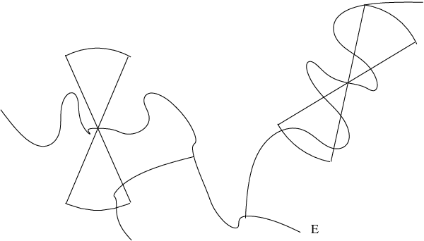
It is easy to verify that is measurable with respect to . In the next section we shall establish the following somewhat technical result.
Proposition 5.3 (Normal directions negligible).
Let the notation and hypotheses be as in Theorem 1.13. There exists a scale index and a Lipschitz constant such that
Let us assume Proposition 5.3 for now, and see how it implies Theorem 1.13. If we let be the space of “good” or “non-normal” directions
then by (2) it suffices to show that
For each , let denote the set
by Fubini’s theorem, it thus suffices to show that
| (25) |
for all .
Fix . We first get rid of an exceptional set. By (8) we can find a finite collection of open balls with radius between and which cover , such that
| (26) |
If is such a ball, we say that an interval is low-density relative to and if and
| (27) |
where is the interval with the same centre as but five times the length. We let denote the union of all the sets generated by balls and intervals which are low-density relative to and .
Lemma 5.4.
We have .
Proof.
By (8) it suffices to show that
for all , where is the collection of all the intervals which are low-density relative to and . By monotone convergence (and the separability of ), it suffices to show this with replaced by any finite subcollection of such intervals. We can also clearly restrict attention to those which intersect . Using Wiener’s Vitali-type covering lemma22 2 This lemma asserts that given any finite collection of balls , one can find a subcollection of disjoint balls such that the dilates cover ., we can then cover this subcollection by for some disjoint in which intersect . But by hypothesis (27) we have
for all . Since the are disjoint, have length at most , and intersect , we see that . Summing the previous estimate in we obtain the claim. ∎
We now use rotational symmetry to normalise . Let . In view of the above lemma, we see that to show (25) it suffices to show that
| (28) |
We now make a key geometric observation (cf. [4, Lemma 15.14]), that is behaving very much like a Lipschitz graph:
Lemma 5.5 (Approximate Lipschitz property).
Let be such that . Then . (See Figure 4.)
Proof.
Fix , and define the set
and the quantity
Clearly . To establish the claim, it will suffice (since contains ) to show that . Suppose this is not the case, thus
| (29) |
By definition of , we can thus find such that
| (30) |
in particular, from (29) and (30) we have
| (31) |
Fix this . By the non-normality hypothesis, we have
and
for all , and thus
| (32) |
where
We apply this fact with ; note that (30), (29), (9) clearly ensure that lies in the range .
Let be the interval . From (31) we see that . We claim the set inclusion
| (33) |
Indeed, if is such that , then
and thus by the triangle inequality and (31)
| (34) |
By the triangle inequality, we either have or . If we see from (31), (34) that
which implies from choice of that
Similarly, if then
In either case we obtain (33).

We now modify the standard proof of the well-known result that a partially defined real-valued Lipschitz function extends to a totally defined real-valued Lipschitz function to obtain:
Corollary 5.6 (Explicit rectifiability).
Let be a ball of radius at most . Then there exists a Lipschitz function of Lipschitz constant at most such that for all .
Proof.
We may assume that is non-empty, otherwise there is nothing to prove. If we then define
then the claim easily follows from the previous lemma. ∎
6. Eliminating high multiplicity directions
We now locate some high multiplicity directions of , and show that their direct contribution is negligible. A key new difficulty in the quantitative setting is that the notion of high multiplicity will depend on scale, and we will need the pigeonhole principle (Lemma 1.14) in order to find a favourable scale with which to perform the analysis.
Definition 6.1 (High multiplicity lines).
Let . A line is said to have high multiplicity at a scale index if the set contains a set of cardinality at least which is -separated, thus any two points in are separated by a distance of at least . We let to be the set of all points such that the line is high multiplicity at a scale index .
Because is compact, it is not difficult to show that is also compact. Also, from (7) we clearly have the nesting property
Applying (23) and Lemma 1.14, we may thus find a scale index near which the are stable in the sense that
| (35) |
We now fix this and work entirely within the scale indices
Now we show that near , the have negligible Favard length. In fact we shall show something slightly stronger:
Definition 6.2 (Angular neighbourhoods).
Let and . We define the -angular neighbourhood of to be the set
We define the set
| (36) |
and the slightly smaller set
| (37) |
Lemma 6.3 ( Favard-negligible).
We have
Remark 6.4.
This is a quantitative counterpart of [4, Lemma 18.4].
Proof.
Let us write for brevity. From (8) we can find a collection of balls with radius which cover such that
| (38) |
If a line is high multiplicity at a scale index , then by definition it intersects in points which are -separated. Each of these points is contained in a ball in , where each has radius , thanks to (7), (9); in particular, the are all disjoint. Now let be such that , thus by (7), (9). From elementary geometry (and the fact that all lie in ) we then see that the line then meets each of the dilated balls (defined as the ball with the same centre as and five times the radius) in a line segment of length (see Figure 5). To put it another way, we have
for all . Summing this, we conclude that
for all . By Fubini’s theorem, we conclude that for every we have
Applying (38), we obtain
Integrating this in , we obtain the claim. ∎
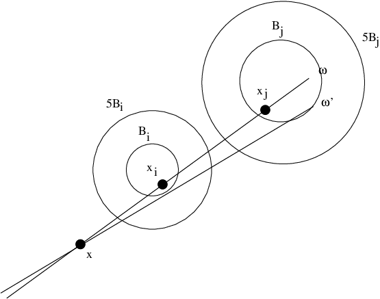
We define the exceptional set
thus from (35) we have that
| (39) |
Because of this, the contribution of will be manageable in the sequel. We make the technical remark that is angularly closed, i.e. for any , the set is closed.
7. Eliminating positive multiplicity directions
In the preceding section we obtained two sets of high multiplicity which were well controlled. Now we perform another scale refinement to also control those directions in which the multiplicity is merely positive, leaving only the zero-multiplicity directions.
Definition 7.1 (Positive multiplicity direction).
Let . We say that a point has positive multiplicity at scale index if the line contains a point in such that . We let be the set of all which have positive multiplicity at scale index .
Suppose that does not lie in , so in particular does not lie in . Applying Definition 6.1, we conclude that contains at most points of which are -separated. Comparing this with Definition 7.1, we see that can lie in at most of the sets . Integrating this and using (23), we conclude that
Applying the pigeonhole principle, we can thus find
such that
| (40) |
Because of this, the contribution of will be manageable in the sequel. Also observe that is closed, and hence is angularly closed in the sense of the preceding section. Henceforth we fix , and work entirely within the scale indices
8. Eliminating high density strips
We now perform a variant of the analysis of the preceding sections, in order to eliminate the contribution of certain strips in which are capturing too much of the mass of .
Definition 8.1 (High density strips).
Let . An infinite strip , where and is an interval, is said to have high density if we have
We let be the set of all points such that the line lies in a high-density strip whose width is at least .
One easily verifies that is compact and that
Restricting to scale indices between and , and then applying (23) and Lemma 1.14, we can locate a scale index such that
| (41) |
Let us now fix this , and work entirely inside the range of scale indices
Lemma 8.2 ( Favard-negligible).
We have
Proof.
By Fubini’s theorem, it suffices to show that
for all .
Fix ; by rotation symmetry we can take , so we need to show
| (42) |
We also abbreviate . Unwrapping the definitions, we see that if , then there exists with and an interval containing with such that
From (7), (9) we have . Also, and lie in the unit ball. From this, we see that , and furthermore if is such that , then . Thus, if we let be the pushforward of the measure to under the projection map , we see that
Since contains , we thus see that the Hardy-Littlewood maximal function of takes the value on . On the other hand, from (23) we see that the total mass of the positive measure is at most . The claim (42) then follows from the Hardy-Littlewood maximal inequality for measures (see e.g. [4, Theorem 2.19]). ∎
9. Conclusion of the argument
Having refined our set of scales suitably, and controlled various exceptional sets, namely two large but coarse sets , and one fine but small set , we are now ready to establish Proposition 5.3.
It will suffice to show that
The key observation is that only consists of points which are close to many points in .
Lemma 9.1.
Let . Then the set
has measure .
Proof.
Fix this . Since is angularly closed, is a compact subset of the circle . Thus we can find a finite number of open arcs in the arc which cover and such that
| (47) |
By enlarging these arcs slightly we can assume that each arc contains at least one point in the complement of ; by concatenating overlapping arcs we may assume that these arcs are disjoint.
Since lies in , it lies outside of , and thus by (37), (36) we have for any . A similar argument gives for any .

Suppose that does not lie in any of the , then by the above discussion does not lie in , , or . In particular we see that does not lie in . This implies that the ray does not intersect . Since is supported on , we conclude
and thus by (46)
| (48) |
On the other hand, given any , we have by construction that there exists at least one which does not lie in . In particular this shows that does not lie in either or , and thus does not lie in . In particular, this shows that
whenever is an interval containing of length . Now, from elementary geometry we see that the double sector can be contained in such a strip with . Thus
for all . Comparing this with (48), (47) we obtain the claim. ∎
From the above lemma, we see that if lies in , then lies in the set where the Hardy-Littlewood maximal function of the indicator function of on the circle is . Applying the Hardy-Littlewood maximal inequality, we conclude that
for all . Integrating this in we obtain
and the claim (45) then follows from Lemma 5.1 and (44). This concludes the proof of Theorem 1.13.
Appendix A -numbers and quantitative unrectifiability
The purpose of this appendix is to use the theory of -numbers to improve the bounds in Proposition 1.20.
Given any dyadic square and compact set , let denote the quantity
where ranges over all lines. Thus for instance when , and also whenever . In [3] it was shown that
whenever is compact and connected, ranges over all dyadic squares, is the length of , and is the square with the same centre as but three times the sidelength. In particular, for a Lipschitz graph with we see that
| (49) |
Proposition A.1 (Rectifiability bound for product Cantor set, II).
If then
Proof.
Once again we can rescale . By enlarging to we can also assume . Let be a Lipschitz graph with , and let , thus
for some closed set . It then suffices to show that . We can assume that is large, since the claim is trivial otherwise. In view of (49), it thus suffices to show that
Let . Then consists of dyadic squares of sidelength ; let be the union of all such squares which intersect , thus
Let , let be one of the squares in , and let be the dyadic squares in of sidelength which are contained in . From elementary geometry we see that if all of these squares lie in , then . Viewing this contrapositively, we see that if then contains at least one square of sidelength contained in . Summing this fact over all in , we see that
A simple counting argument shows that
where denotes two-dimensional Lebesgue measure. Similarly
and thus
Summing in and using telescoping series, we obtain
We can directly compute that . Also, consists of squares of length , and the intersection of each such square with contributes a set of measure to . We thus have
and the claim follows. ∎
The estimate in Proposition A.1 is significantly stronger than that in Proposition 1.20, as the former becomes non-trivial as soon as , whereas the latter is only non-trivial for . However, both estimates, when inserted into Theorem 1.13, give essentially the same result; replacing Proposition 1.20 by Proposition A.1 allows one to reduce the double-exponential in (13) to single-exponential, but after iteration this only affects the (unspecified) implied constant in the final bound for .
References
- [1] A. Besicovitch, On the fundamental geometric properties of linearly measurable plane sets of points III, Math. Ann. 116 (1939), 349–357.
- [2] K. Falconer, The geometry of fractal sets, Cambridge Tracts in Mathematics 85, Cambridge University Press, Cambridge-New York, 1986.
- [3] P. Jones, Rectifiable sets and the travelling salesman problem, Invent. Math. 102 (1990), 1–15.
- [4] P. Mattila, Geometry of Sets and Measures in Euclidean Spaces: Fractals and rectifiability. Cambridge studies in advanced mathematics 44, Cambridge University Press, Cambridge-New York, 1995.
- [5] F. Nazarov, Y. Peres, A. Volberg, preprint.
- [6] K. Okikiolu, Characterization of subsets of rectifiable curves in , J. London Math. Soc. 46 (1992), 336–348.
- [7] Y. Peres, B. Solomyak, How likely is Buffon’s needle to fall near a planar Cantor set?, Pacific J. Math. 204 (2002), 473–496.