跳到论文正文
W Papers独立论文阅读器 arXiv:0706.2635 论文正文 计算阅读时间 · 0%
引用这篇论文根据当前论文元数据生成,正式投稿前建议核对。


License: Assumed arXiv.org perpetual non-exclusive license
arXiv:0706.2635v2 [cond-mat.mes-hall] 21 Sep 2007
\lat\rtitle

Magnetic flux detection with an Andreev Quantum Dot \sodtitleMagnetic flux detection with an Andreev Quantum Dot \rauthorI.A. Sadovskyy, G.B. Lesovik, G. Blatter \sodauthorSadovskyy, Lesovik, Blatter \dates25 May 2007*

\PACS

73.21.La, 74.45.+c, 07.55.Ge

Magnetic flux detection with an Andreev Quantum Dot

I.A. Sadovskyy∗ Thanks: sadovsky@itp.ac.ru    G.B. Lesovik∗    G. Blatter∇ Address: ∗L.D. Landau Institute for Theoretical Physics, Russian Academy of Sciences, 119334, Kosygina st., 2, Moscow, Russia
∇Theoretische Physik, Schafmattstrasse 32, ETH-Zurich, CH-8093 Zürich, Switzerland
Abstract

The charge of the subgap states in an Andreev quantum dot (AQD; this is a quantum dot inserted into a superconducting loop) is very sensitive to the magnetic flux threading the loop. We study the sensitivity of this device as a function of its parameters for the limit of a large superconducting gap Δ\Delta. In our analysis, we account for the effects of a weak Coulomb interaction within the dot. We discuss the suitability of this setup as a device detecting weak magnetic fields.

Introduction.

The Josephson effect [1] has been intensively studied during the past 45 years; its main characteristic is the presence of a tunable non-dissipative current when two bulk superconductors are joined via a normal or insulating layer and subjected to a superconducting phase difference φ\varphi. Recently, it has been realized that in a metallic junction the charge of the normal island in between the superconducting leads depends on the superconducting phase difference φ\varphi as well [3, 2]. This dependence is sufficiently strong [3] to use this effect in a magnetic flux detector, although our estimates below give a sensitivity somewhat below the sensitivity of the best SQUIDs.

Usually, small magnetic fields are measured by superconducting quantum interference devices (SQUIDs) [4, 5]. While SQUIDs are based on the dependence of the Josephson current on the superconducting phase difference φ\varphi (and hence on the magnetic flux Φ\Phi threading the loop), here we propose to use the charge-dependence in an Andreev quantum dot for the flux measurement. As shown in Ref. [3], the charge QQ of a single-channel Andreev quantum dot can be fractional −|e|<Q<|e|-|e|<Q<|e| and depends on φ\varphi (here e=−|e|e=-|e| is the charge of one electron).

The charge of an Andreev quantum dot can be measured by a sensitive charge detector, e.g., by a single-electron transistor (SET). Today, the best single electron transistors have a sensitivity of the order of 10−5​|e|/Hz10^{-5}\,|e|/\sqrt{\mathrm{Hz}} (e.g., see [6]). Using results of Ref. [3], simple estimates tell that an AQD can convert a change in flux δ​Φ\delta\Phi to a change in charge δ​Q\delta Q with a ratio δ​Q/δ​Φ∼2​|e|/Φ0\delta Q/\delta\Phi\sim 2|e|/\Phi_{0}, where Φ0=2​π​ℏ/2​|e|\Phi_{0}=2\pi\hbar/2|e| is the superconducting flux. Assuming a superconducting loop area ∼1\sim 1 mm2, we obtain the sensitivity 10−14​T/Hz10^{-14}\,\mathrm{T}/\sqrt{\mathrm{Hz}}, which is comparable with the sensitivity 10−14÷10−15​T/Hz10^{-14}\div 10^{-15}\,\mathrm{T}/\sqrt{\mathrm{Hz}} of today’s best SQUIDs [4, 5]. Below, we study in detail the sensitivity ratio δ​Q/δ​Φ\delta Q/\delta\Phi.

Setup.

Refer to caption

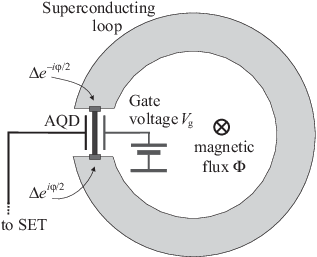
Figure 1: Fig. 1. Andreev quantum dot inserted into the superconducting loop. The Andreev quantum dot is connected to a single electron transistor (SET) and a gate electrode through capacitive couplings. The flux Φ\Phi produces a phase difference φ=2​π​Φ/Φ0\varphi=2\pi\Phi/\Phi_{0} across the Andreev quantum dot. The charge of the AQD can be tuned by the gate voltage VgV_{\mathrm{g}} and the flux Φ\Phi threading the loop.

Our Andreev quantum dot is realized by a small metallic dot connecting two superconducting banks joined in a loop, see Fig. 1. Our AQD is assumed to be a quasi one-dimensional normal metal (N) island separated from the superconductors (S) by thin insulator layers (I), generating normal scattering on top of the Andreev scattering characteristic of the normal-metal superconductor junction. The position of the normal resonance in this SINIS system can be tuned by the gate voltage VgV_{\mathrm{g}} applied to the normal region of the AQD. The magnetic flux threading the loop Φ\Phi induces a superconducting phase drop φ\varphi across the AQD. Since the phase drop in the bulk superconductor is negligible as compared to the phase drop φ\varphi across the AQD one may relate the latter to the flux Φ\Phi threading the loop, φ=2​π​Φ/Φ0\varphi=2\pi\Phi/\Phi_{0}. In order to measure the charge trapped on the AQD, a single electron transistor is capacitively coupled to the normal metal island. Experimentally, such AQDs have recently been fabricated by coupling carbon nanotubes to superconducting banks [7, 8, 9, 10]. In the following, we concentrate on the properties of the key element in the setup — the Andreev quantum dot.

Energy and charge of the AQD without Coulomb interaction

The Andreev states give rise to new opportunities for tunable Josephson devices, e.g., the Josephson transistor [11, 12, 13]; here, we are interested in their charge properties. We will consider the case of one transverse channel such that the problem effectively becomes one dimensional. We consider the case of a large separation δN\delta_{\rm\scriptscriptstyle N} between the resonances in the associated NININ problem (where the superconductors S have been replaced by normal metal leads N), δN≫Δ\delta_{\rm\scriptscriptstyle N}\gg\Delta, such that a single Andreev level εA\varepsilon_{\rm\scriptscriptstyle A} is trapped within the gap region. We are interested in sufficiently well isolated dots with a small width ΓN\Gamma_{\rm\scriptscriptstyle N} of the associated NININ resonance, ΓN≪Δ\Gamma_{\rm\scriptscriptstyle N}\ll\Delta. In this section, we neglect charging effects EC=0E_{\rm\scriptscriptstyle C}=0. In summary, our device operates with energy scales ΓN≪Δ≪δN\Gamma_{\rm\scriptscriptstyle N}\ll\Delta\ll\delta_{\rm\scriptscriptstyle N}.

The resonances in the NININ setup derive from the eigenvalue problem ℋ^0​Ψ=E​Ψ\mathcal{\hat{H}}_{0}\Psi=E\Psi with ℋ^0=−ℏ2∂x2/2m+U(x)−εF\mathcal{\hat{H}}_{0}=-\hbar^{2}\partial_{x}^{2}/2m+U(x)-\varepsilon_{\rm\scriptscriptstyle F} with the potential U(x)=Ups, 1(x+L/2)+Ups, 2(x−L/2)]+eVgθ(L/2−|x|)]U(x)=U_{\mathrm{ps,\,1}}(x+L/2)+U_{\mathrm{ps,\,2}}(x-L/2)]+eV_{\mathrm{g}}\theta(L/2-|x|)] describing two point-scatterers11 1 The Heaviside function θ⁡(x)=1\theta(x)=1 for x>0x>0 and θ⁡(x)=0\theta(x)=0 for x⩽0x\leqslant 0. (with transmission and reflection amplitudes Tl1/2​eχltT_{l}^{1/2}e^{\chi^{t}_{l}}, Rl1/2​eχlrR_{l}^{1/2}e^{\chi^{r}_{l}}; Rl=1−TlR_{l}=1-T_{l}, l=1,l=1, 22) and the effect of the gate potential VgV_{\mathrm{g}}, which we assume to be small as compared to the particle’s energy EE (measured from the band bottom in the leads), e​Vg≪EeV_{\mathrm{g}}\ll E. Resonances then appear at energies En=εL​(n​π−χ1r/2−χ2r/2)2E_{n}=\varepsilon_{L}(n\pi-\chi^{r}_{1}/2-\chi^{r}_{2}/2)^{2}; they are separated by δNn=(En+1−En−1)/2≈2​En/n\delta_{\rm\scriptscriptstyle N}^{n}=(E_{n+1}-E_{n-1})/2\approx 2E_{n}/n and are characterized by the width ΓNn=T​δNn/π​R\Gamma_{\rm\scriptscriptstyle N}^{n}=T\delta_{\rm\scriptscriptstyle N}^{n}/\pi\sqrt{R}, where εL=ℏ2/2​m​L2\varepsilon_{L}=\hbar^{2}/2mL^{2}. The bias VgV_{\mathrm{g}} shifts the resonances by e​VgeV_{\mathrm{g}}; we denote the position of the nn-th resonance relative to εF\varepsilon_{\rm\scriptscriptstyle F} by εNn=En+e​Vg−εF\varepsilon_{\rm\scriptscriptstyle N}^{n}=E_{n}+eV_{\mathrm{g}}-\varepsilon_{\rm\scriptscriptstyle F}. In the following, we choose a specific resonance in the gap by selecting an appropriate nn and drop the index nn, εNn→εN\varepsilon_{\rm\scriptscriptstyle N}^{n}\to\varepsilon_{\rm\scriptscriptstyle N}, δNn→δN\delta_{\rm\scriptscriptstyle N}^{n}\to\delta_{\rm\scriptscriptstyle N}, ΓNn→ΓN\Gamma_{\rm\scriptscriptstyle N}^{n}\to\Gamma_{\rm\scriptscriptstyle N}.

We go from a normal- to an Andreev dot by replacing the normal leads with superconducting ones. In order to include Andreev scattering in the SINIS setup, we have to solve the Bogoliubov-de Gennes equations (we choose states with εA⩾0\varepsilon_{\rm\scriptscriptstyle A}\geqslant 0)

[ℋ^0​(x)Δ^​(x)Δ^∗​(x)−ℋ^0​(x)]​[uv]=εA​[uv],\displaystyle\left[\begin{array}[]{cc}\mathcal{\hat{H}}_{0}(x)&{\hat{\Delta}}(x)\\ {\hat{\Delta}}^{*}(x)&-\mathcal{\hat{H}}_{0}(x)\end{array}\right]\!\left[\begin{array}[]{c}\!\!u\\ \!\!v\end{array}\right]=\varepsilon_{\rm\scriptscriptstyle A}\left[\begin{array}[]{c}\!\!u\\ \!\!v\end{array}\right],

with the pairing potential Δ^(x)=Δ[θ(−x−L/2)e−iφ/2+θ(x−L/2)ei​φ/2]{\hat{\Delta}}(x)=\Delta[\theta(-x-L/2)e^{-i\varphi/2}+\theta(x-L/2)e^{i\varphi/2}]; u⁡(x)u(x) and v⁡(x)v(x) are the electron- and hole-like components of the wave function. The discrete states trapped below the gap derive from the quantization condition (in Andreev approximation)

(R1+R2)​cos⁡(2​π​εAδN)−4​R1​R2​sin2⁡α​cos⁡(2​π​εNδ​N)++T1​T2​cos⁡φ=cos⁡(2​α−2​π​εAδN)+R1​R2​cos⁡(2​α+2​π​εAδN).(R_{1}+R_{2})\cos\!\Big(2\pi\frac{\varepsilon_{\rm\scriptscriptstyle A}}{\delta_{\rm\scriptscriptstyle N}}\Big)-4\sqrt{R_{1}R_{2}}\,\sin^{2}\alpha\,\cos\!\Big(2\pi\frac{\varepsilon_{\rm\scriptscriptstyle N}}{\delta{\rm\scriptscriptstyle N}}\Big)+\\ +T_{1}T_{2}\cos\varphi=\cos\!\Big(2\alpha-2\pi\frac{\varepsilon_{\rm\scriptscriptstyle A}}{\delta_{\rm\scriptscriptstyle N}}\Big)+R_{1}R_{2}\cos\!\Big(2\alpha+2\pi\frac{\varepsilon_{\rm\scriptscriptstyle A}}{\delta_{\rm\scriptscriptstyle N}}\Big). (8)

The phase α=arccos⁡(εA/Δ)\alpha=\arccos(\varepsilon_{\rm\scriptscriptstyle A}/\Delta) is acquired at an ideal NS boundary due to Andreev reflection with φ=0\varphi=0; the above formula can be directly obtained using results from Refs. [13, 14].

We concentrate on the regime ΓN,|εN|≪Δ\Gamma_{\rm\scriptscriptstyle N},|\varepsilon_{\rm\scriptscriptstyle N}|\ll\Delta, the so-called Δ→∞\Delta\to\infty limit. In this limit, the quantization condition can be expanded and we obtain the expression (AA is the asymmetry parameter)

εA=εN2+εΓ2,\varepsilon_{\rm\scriptscriptstyle A}=\sqrt{\varepsilon_{\rm\scriptscriptstyle N}^{2}+\varepsilon_{\rm\scriptscriptstyle\Gamma}^{2}}, (9)

where

εΓ=ΓN2​cos2⁡φ2+A2,A=|T1−T2|2​T1​T2.\varepsilon_{\rm\scriptscriptstyle\Gamma}=\frac{\Gamma_{\rm\scriptscriptstyle N}}{2}\sqrt{\cos^{2}\frac{\varphi}{2}+A^{2}},\;\;\;A=\frac{|T_{1}-T_{2}|}{2\sqrt{T_{1}T_{2}}}. (10)

The energy εA\varepsilon_{\rm\scriptscriptstyle A} of the Andreev state is phase sensitive when εN\varepsilon_{\rm\scriptscriptstyle N} is close to the chemical potential, |εN|≲ΓN|\varepsilon_{\rm\scriptscriptstyle N}|\lesssim\Gamma_{\rm\scriptscriptstyle N}, which can be achieved by tuning the gate potential VgV_{\mathrm{g}}. In the limit Δ→∞\Delta\to\infty, both the u⁡(x)u(x) and v⁡(x)v(x) components of the wave function are nonzero only in the normal region,

[u⁡(x)v⁡(x)]={0,|x|>L/2,[Ce→​ei​ke​x+Ce←​e−i​ke​xCh←​ei​kh​x+Ch→​e−i​kh​x],|x|<L/2,\left[\begin{array}[]{c}\!\!u(x)\\ \!\!v(x)\end{array}\right]=\left\{\begin{array}[]{cl}0,&\!|x|>L/2,\\ \left[\begin{array}[]{c}\!\!C^{\rightarrow}_{\mathrm{e}}e^{ik_{\mathrm{e}}x}+C^{\leftarrow}_{\mathrm{e}}e^{-ik_{\mathrm{e}}x}\\ \!\!C^{\leftarrow}_{\mathrm{h}}e^{ik_{\mathrm{h}}x}+C^{\rightarrow}_{\mathrm{h}}e^{-ik_{\mathrm{h}}x}\end{array}\right]\!,&\!|x|<L/2,\end{array}\right.

where ke,h=[2​m​(εF±εA)]1/2/ℏk_{\mathrm{e},\mathrm{h}}=[2m(\varepsilon_{\rm\scriptscriptstyle F}\pm\varepsilon_{\rm\scriptscriptstyle A})]^{1/2}/\hbar are the wave vectors of electrons and holes, respectively. The coefficients are defined by Ce,h→=Ce,h←=[(1±εN/εA)/4​L]1/2C^{\rightarrow}_{\mathrm{e,h}}=C^{\leftarrow}_{\mathrm{e,h}}=[(1\pm\varepsilon_{\rm\scriptscriptstyle N}/\varepsilon_{\rm\scriptscriptstyle A})/4L]^{1/2}.

The ground state of the system is the state |0⟩|0\rangle with energy

ε0=εN−εA\varepsilon_{0}=\varepsilon_{\rm\scriptscriptstyle N}-\varepsilon_{\rm\scriptscriptstyle A} (11)

(counted from the Fermi energy εF\varepsilon_{\rm\scriptscriptstyle F}), where we have subtracted the energy of filled resonances below the Fermi surface; the latter are not modified by the superconductivity in the leads and hence do not depend on the phase φ\varphi. The first excited state with one Bogoliubov quasiparticle is doubly degenerate in spin |1↑⟩=a^↑†​|0⟩|1_{\uparrow}\rangle={\hat{a}}_{\uparrow}^{\dagger}|0\rangle, |1↓⟩=a^↓†​|0⟩|1_{\downarrow}\rangle={\hat{a}}_{\downarrow}^{\dagger}|0\rangle and has energy ε1=ε0+εA=εN\varepsilon_{1}=\varepsilon_{0}+\varepsilon_{\rm\scriptscriptstyle A}=\varepsilon_{\rm\scriptscriptstyle N}. The doubly excited state with two quasiparticles |2⟩=a^↑†​a^↓†​|0⟩|2\rangle={\hat{a}}_{\uparrow}^{\dagger}{\hat{a}}_{\downarrow}^{\dagger}|0\rangle has an energy ε2=ε0+2​εA=εN+εA\varepsilon_{2}=\varepsilon_{0}+2\varepsilon_{\rm\scriptscriptstyle A}=\varepsilon_{\rm\scriptscriptstyle N}+\varepsilon_{\rm\scriptscriptstyle A}.

The charge of the state |ν⟩|\nu\rangle (ν=0\nu=0, 1↑1_{\uparrow}, 1↓1_{\downarrow}, 22) can be obtained by differentiation of the corresponding energy εν\varepsilon_{\nu} with respect to the gate voltage, qν=∂εν/∂Vgq_{\nu}=\partial\varepsilon_{\nu}/\partial V_{\mathrm{g}}, or by averaging the charge operator Q^=e∑σ∫−L/2L/2Ψ^σ†(x)Ψ^σ(x)dx{\hat{Q}}=e\sum_{\sigma}\int_{-L/2}^{L/2}{\hat{\Psi}}_{\sigma}^{\dagger}(x){\hat{\Psi}}_{\sigma}^{\phantom{{\dagger}}}(x)\,dx over the state |ν⟩|\nu\rangle, qν=⟨ν|Q^|ν⟩q_{\nu}=\langle\nu|{\hat{Q}}|\nu\rangle. Both methods give the identical results

q0=e(1−εNεA),q1=e,q2=e(1+εNεA).q_{0}=e\Big(1-\frac{\varepsilon_{\rm\scriptscriptstyle N}}{\varepsilon_{\rm\scriptscriptstyle A}}\Big),\;q_{1}=e,\;q_{2}=e\Big(1+\frac{\varepsilon_{\rm\scriptscriptstyle N}}{\varepsilon_{\rm\scriptscriptstyle A}}\Big). (12)

Below, we will also need the off-diagonal matrix elements of the charge operator Q^{\hat{Q}}; the only non-vanishing term is q02=⟨0|Q^|2⟩=e​(1−εN2/εA2)1/2q_{02}=\langle 0|{\hat{Q}}|2\rangle=e(1-\varepsilon_{\rm\scriptscriptstyle N}^{2}/\varepsilon_{\rm\scriptscriptstyle A}^{2})^{1/2}.

AQD with Coulomb interaction

Refer to caption

Figure 2: Fig. 2. Energies E−E_{-} (solid line), E1E_{1} (dashed line), and E+E_{+} (dotted line) are plotted versus the position of normal resonance. All energies are given in units of εΓ\varepsilon_{\rm\scriptscriptstyle\Gamma}, cf. (10). The Coulomb energy is EC=0E_{\rm\scriptscriptstyle C}=0 for (a), EC=εΓE_{\rm\scriptscriptstyle C}=\varepsilon_{\rm\scriptscriptstyle\Gamma} for (b), EC=2​εΓE_{\rm\scriptscriptstyle C}=2\varepsilon_{\rm\scriptscriptstyle\Gamma} for (c), and EC=3​εΓE_{\rm\scriptscriptstyle C}=3\varepsilon_{\rm\scriptscriptstyle\Gamma} for (d). In accordance with formula (26) the doublet region appears when EC>εΓE_{\rm\scriptscriptstyle C}>\varepsilon_{\rm\scriptscriptstyle\Gamma}, see (b–d). In the filled region the ground state of the system is a doublet; the width of this region is 2​(EC2−εΓ2)1/22(E_{\rm\scriptscriptstyle C}^{2}-\varepsilon_{\rm\scriptscriptstyle\Gamma}^{2})^{1/2}, the edges of this region are spread due to the finite temperature Θ\Theta.

In order to find the effect of weak Coulomb interaction EC≪ΔE_{\rm\scriptscriptstyle C}\ll\Delta in the limit ΓN,\Gamma_{\rm\scriptscriptstyle N}, |εN|≪Δ|\varepsilon_{\rm\scriptscriptstyle N}|\ll\Delta, we can disregard the continuous states with energies above the superconducting gap Δ\Delta and assume that the four levels of the discrete spectrum form the entire basis of the system’s Hilbert space22 2 In realistic nanodevices the Coulomb energy can be larger then ΓN\Gamma_{\rm\scriptscriptstyle N} and smaller or of the order of δN\delta_{\rm\scriptscriptstyle N}, but in principle can be made much smaller than both δN\delta_{\rm\scriptscriptstyle N} and Δ\Delta (see the discussion in [7, 3]).. The interaction is given by the operator

V^=EC​Q^2e2.{\hat{V}}=E_{\rm\scriptscriptstyle C}\frac{{\hat{Q}}^{2}}{e^{2}}. (13)

Given the basis with these four states, we can diagonalize the Hamiltonian exactly. The non-zero matrix elements of the operator V^{\hat{V}} are

V00=EC(q02+q022)/e2,V11=EC,V22=EC(q22+q022)/e2,V02=2ECq02/e.V_{00}=E_{\rm\scriptscriptstyle C}(q_{0}^{2}+q_{02}^{2})/e^{2},\;V_{11}=E_{\rm\scriptscriptstyle C},\;\\ V_{22}=E_{\rm\scriptscriptstyle C}(q_{2}^{2}+q_{02}^{2})/e^{2},\;V_{02}=2E_{\rm\scriptscriptstyle C}q_{02}/e. (14)

The energy levels are defined by the eigenvalue problem

[ε~0−EV02ε~1↑−Eε~1↓−EV20ε~2−E]​[D0D1↑D1↓D2]=0,\displaystyle\left[\begin{array}[]{cccc}\!\!{\tilde{\varepsilon}}_{0}-E&&&\!\!V_{02}\\ &\!\!{\tilde{\varepsilon}}_{1\uparrow}-E&&\\ &&\!\!{\tilde{\varepsilon}}_{1\downarrow}-E&\\ \!\!V_{20}&&&\!\!{\tilde{\varepsilon}}_{2}-E\\ \end{array}\right]\!\left[\begin{array}[]{l}\!\!D_{0}\\ \!\!D_{1\uparrow}\\ \!\!D_{1\downarrow}\\ \!\!D_{2}\end{array}\right]=0,

where ε~ν=εν+Vν​ν{\tilde{\varepsilon}}_{\nu}=\varepsilon_{\nu}+V_{\nu\nu}, ν=0\nu=0, 1↑1_{\uparrow}, 1↓1_{\downarrow}, 22. The energy of the level with one Bogoliubov quasiparticle |1⟩|1\rangle is given by the (shifted) constant

E1=εN+EC,E_{1}=\varepsilon_{\rm\scriptscriptstyle N}+E_{\rm\scriptscriptstyle C}, (24)

and does not mix with the other states; furthermore, the spin degeneracy of this Kramers doublet remains. The ground state |0⟩|0\rangle and the doubly excited state |2⟩|2\rangle mix due to Coulomb interaction and produce two new states, the singlet states |−⟩|-\rangle and |+⟩|+\rangle; |±⟩=D0±​|0⟩+D2±​|2⟩|\pm\rangle=D_{0}^{\pm}|0\rangle+D_{2}^{\pm}|2\rangle, D0±/D2±=−V02/(ε~0−E±)D_{0}^{\pm}/D_{2}^{\pm}=-V_{02}/({\tilde{\varepsilon}}_{0}-E_{\pm}), |D0±|2+|D2±|2=1|D_{0}^{\pm}|^{2}+|D_{2}^{\pm}|^{2}=1. The energies of these new states are

E±=εN+2​EC±(εN+2​EC)2+εΓ2.E_{\pm}=\varepsilon_{\rm\scriptscriptstyle N}+2E_{\rm\scriptscriptstyle C}\pm\sqrt{(\varepsilon_{\rm\scriptscriptstyle N}+2E_{\rm\scriptscriptstyle C})^{2}+\varepsilon_{\rm\scriptscriptstyle\Gamma}^{2}}. (25)

The energies of the doublet and singlet states depend on εN\varepsilon_{\rm\scriptscriptstyle N} and φ\varphi in a different way and may cross; thus the ground state can be formed by either the singlet |−⟩|-\rangle or by the doublet |1⟩|1\rangle. The state |+⟩|+\rangle always remains the second excited state, see Fig. 2. When EC>εΓ⩾ΓN​A/2≡EC∗E_{\rm\scriptscriptstyle C}>\varepsilon_{\rm\scriptscriptstyle\Gamma}\geqslant\Gamma_{\rm\scriptscriptstyle N}A/2\equiv E_{\rm\scriptscriptstyle C}^{*} (with AA the asymmetry parameter) the ground state is the doublet |1⟩|1\rangle in the region

−2​EC−EC2−εΓ2<εN<−2​EC+EC2−εΓ2-2E_{\rm\scriptscriptstyle C}-\sqrt{E_{\rm\scriptscriptstyle C}^{2}-\varepsilon_{\rm\scriptscriptstyle\Gamma}^{2}}<\varepsilon_{\rm\scriptscriptstyle N}<-2E_{\rm\scriptscriptstyle C}+\sqrt{E_{\rm\scriptscriptstyle C}^{2}-\varepsilon_{\rm\scriptscriptstyle\Gamma}^{2}} (26)

and remains |−⟩|-\rangle at all other values of εN\varepsilon_{\rm\scriptscriptstyle N} [15].

The origin of this level crossing can be traced to the different shifts in energies with ECE_{\rm\scriptscriptstyle C}: While E1E_{1} is shifted up by ECE_{\rm\scriptscriptstyle C}, E−E_{-} quickly approaches 0 with increasing ECE_{\rm\scriptscriptstyle C}. Note that the terms ∝q022\propto q_{02}^{2} and ∝q02\propto q_{02} in the matrix elements Vν​ν′V_{\nu\nu^{\prime}} lead to the crossing of the energies E−E_{-} and E1E_{1}, while preventing the crossing of the level E+E_{+} with the others.

At the edge of the region (26) a sharp singlet to doublet crossover takes place, with a jump appearing as a function of εN​(Vg)\varepsilon_{\rm\scriptscriptstyle N}(V_{\mathrm{g}}) or εΓ​(φ)\varepsilon_{\rm\scriptscriptstyle\Gamma}(\varphi) in the charge of the Andreev dot and in the current across (see below).

Refer to caption

Figure 3: Fig. 3. Equilibrium charge QeqQ_{\mathrm{eq}} (29) versus superconducting phase difference φ\varphi. In (a) and (b) the temperature is zero (i.e., QeqQ_{\mathrm{eq}} represents ground state charge), in (c) and (d) the temperature is Θ=0.1​EC∗\Theta=0.1E_{\rm\scriptscriptstyle C}^{*}, where EC∗≡ΓN​A/2E_{\rm\scriptscriptstyle C}^{*}\equiv\Gamma_{\rm\scriptscriptstyle N}A/2. The Coulomb energy is EC=1.2​EC∗E_{\rm\scriptscriptstyle C}=1.2E_{\rm\scriptscriptstyle C}^{*} for (a) and (c), EC=2.0​EC∗E_{\rm\scriptscriptstyle C}=2.0E_{\rm\scriptscriptstyle C}^{*} for (b) and (d). The asymmetry level of the dot is A=0.2A=0.2. The features in the center of the plots corresponds to the Kramers doublet region (26). In (c) and (d) the border of the doublet region is smoothed by the temperature Θ\Theta.

The charges of the new states |μ⟩|\mu\rangle, (μ=1,\mu=1, ±\pm) can be calculated as in the previous section, Qμ=∂Eμ/∂VgQ_{\mu}=\partial E_{\mu}/\partial V_{\mathrm{g}}, and are given by

Q±=e⁡(1±εN+2​EC(εN+2​EC)2+εΓ2),Q1=e.Q_{\pm}=e\bigg(1\pm\frac{\varepsilon_{\rm\scriptscriptstyle N}+2E_{\rm\scriptscriptstyle C}}{\sqrt{(\varepsilon_{\rm\scriptscriptstyle N}+2E_{\rm\scriptscriptstyle C})^{2}+\varepsilon_{\rm\scriptscriptstyle\Gamma}^{2}}}\bigg),\;\;\;Q_{1}=e. (27)

The charge Q1Q_{1} is integer and does not fluctuate; the charges Q±Q_{\pm} are fractional in the region |εN+2​EC|∼εΓ|\varepsilon_{\rm\scriptscriptstyle N}+2E_{\rm\scriptscriptstyle C}|\sim\varepsilon_{\rm\scriptscriptstyle\Gamma} and fluctuate strongly (see also the discussion of fluctuations in Ref. [3] where Coulomb effects have been ignored)

δ​Q±≡[⟨±Q^2​|±⟩−⟨±Q^|±⟩2]1/2==e​εΓ(εN+2​EC)2+εΓ2.\delta Q_{\pm}\equiv[\langle\pm{\hat{Q}}^{2}|\pm\rangle-\langle\pm{\hat{Q}}|\pm\rangle^{2}]^{1/2}=\\ =e\frac{\varepsilon_{\rm\scriptscriptstyle\Gamma}}{\sqrt{(\varepsilon_{\rm\scriptscriptstyle N}+2E_{\rm\scriptscriptstyle C})^{2}+\varepsilon_{\rm\scriptscriptstyle\Gamma}^{2}}}. (28)

Note that the Coulomb interaction merely shifts the regime of εN\varepsilon_{\rm\scriptscriptstyle N} where the charges Q±Q_{\pm} are fractional. Everywhere outside the doublet region the ground state charge is given by Q−Q_{-}, while within the Kramers doublet region the charge is pinned to the value Q1=eQ_{1}=e. As illustrated in Figs. 3a and 3b, for EC>EC∗E_{\rm\scriptscriptstyle C}>E_{\rm\scriptscriptstyle C}^{*} a sharp crossover occurs and the charge jumps by the value δ​Qcr=Q−−Q1\delta Q_{\mathrm{cr}}=Q_{-}-Q_{1}. This jump is smeared at finite temperatures, see Figs. 3c and 3d. The groundstate charge is

Qgs=e−eENEAθ[EC<EA],Q_{\mathrm{gs}}=e-e\frac{E_{\rm\scriptscriptstyle N}}{E_{\rm\scriptscriptstyle A}}\,\theta[E_{\rm\scriptscriptstyle C}<E_{\rm\scriptscriptstyle A}],

where EA=[(εN+2​EC)2+εΓ2]1/2E_{\rm\scriptscriptstyle A}=[(\varepsilon_{\rm\scriptscriptstyle N}+2E_{\rm\scriptscriptstyle C})^{2}+\varepsilon_{\rm\scriptscriptstyle\Gamma}^{2}]^{1/2} and EN=εN+2​ECE_{\rm\scriptscriptstyle N}=\varepsilon_{\rm\scriptscriptstyle N}+2E_{\rm\scriptscriptstyle C} denotes the energy of the shifted normal state resonance. The equilibrium charge at finite temperature Θ\Theta is

Qeq=Q−e−E−/Θ+2Q1e−E1/Θ+Q+e−E+/Θe−E−/Θ+2e−E1/Θ+e−E+/Θ;Q_{\mathrm{eq}}=\frac{Q_{-}e^{-E_{-}/\Theta}+2Q_{1}e^{-E_{1}/\Theta}+Q_{+}e^{-E_{+}/\Theta}}{e^{-E_{-}/\Theta}+2e^{-E_{1}/\Theta}+e^{-E_{+}/\Theta}}; (29)

here and below we set Boltzmann’s constant kB=1k_{\rm\scriptscriptstyle B}=1. The equilibrium charge as a function of the superconducting phase φ=2​π​Φ/Φ0\varphi=2\pi\Phi/\Phi_{0} is shown in Fig. 3.

The currents in the states |μ⟩|\mu\rangle are defined by relationship Jμ=∂Eμ/∂ΦJ_{\mu}=\partial E_{\mu}/\partial\Phi which provides the results

J±=∓2​πΦ0​ΓN2​sin⁡φ16​EA,J1=0.J_{\pm}=\mp\frac{2\pi}{\Phi_{0}}\frac{\Gamma_{\rm\scriptscriptstyle N}^{2}\sin\varphi}{16E_{\rm\scriptscriptstyle A}},\;\;\;J_{1}=0. (30)

The groundstate current is

Jgs=2​πΦ0ΓN2​sin⁡φ16​EAθ[EC<EA];J_{\mathrm{gs}}=\frac{2\pi}{\Phi_{0}}\frac{\Gamma_{\rm\scriptscriptstyle N}^{2}\sin\varphi}{16E_{\rm\scriptscriptstyle A}}\,\theta[E_{\rm\scriptscriptstyle C}<E_{\rm\scriptscriptstyle A}];

note that the current vanishes throughout the doublet region. The thermal equilibrium current is

Jeq=J−e−E−/Θ+J+e−E+/Θe−E−/Θ+2e−E1/Θ+e−E+/Θ.J_{\mathrm{eq}}=\frac{J_{-}e^{-E_{-}/\Theta}+J_{+}e^{-E_{+}/\Theta}}{e^{-E_{-}/\Theta}+2e^{-E_{1}/\Theta}+e^{-E_{+}/\Theta}}. (31)

Differential sensitivity

The differential sensitivity of the equilibrium charge to the magnetic flux threading the superconducting loop is defined by the absolute value of the derivative ∂Qeq/∂Φ\partial Q_{\mathrm{eq}}/\partial\Phi taken at the given value of flux,33 3 Note that the sensitivity of the charge-to-flux convertor S≡SΦ→QS\equiv S_{{\rm\scriptscriptstyle\Phi}\to{\rm\scriptscriptstyle Q}} coincides with the voltage-to-current sensitivity of the Josephson transistor described in Ref. [13] SV→J=|∂Jeq/∂Vg|S_{{\rm\scriptscriptstyle V}\to{\rm\scriptscriptstyle J}}=|\partial J_{\mathrm{eq}}/\partial V_{\mathrm{g}}|. S=|∂Qeq/∂Φ|S=|\partial Q_{\mathrm{eq}}/\partial\Phi|. By using (29) we obtain

S=|FΘ​∂Q∂Φ+Q​∂FΘ∂Φ|,S=\left|F_{\Theta}\,\frac{\partial Q}{\partial\Phi}+Q\,\frac{\partial F_{\Theta}}{\partial\Phi}\right|, (32)

where Q≡(Q+−Q−)/2Q\equiv(Q_{+}-Q_{-})/2, the derivative

∂Q∂Φ=e​2​πΦ0​EN​ΓN2​sin⁡φ16​EA3,\frac{\partial Q}{\partial\Phi}=e\frac{2\pi}{\Phi_{0}}\,\frac{E_{\rm\scriptscriptstyle N}\Gamma_{\rm\scriptscriptstyle N}^{2}\sin\varphi}{16E_{\rm\scriptscriptstyle A}^{3}}, (33)

the function

FΘ=e−E+/Θ−e−E−/Θe−E−/Θ+2e−E1/Θ+e−E+/Θ==−sinh⁡(EA/Θ)cosh⁡(EA/Θ)+eEC/Θ,F_{\Theta}=\frac{e^{-E_{+}/\Theta}-e^{-E_{-}/\Theta}}{e^{-E_{-}/\Theta}+2e^{-E_{1}/\Theta}+e^{-E_{+}/\Theta}}=\\ =-\frac{\sinh(E_{\rm\scriptscriptstyle A}/\Theta)}{\cosh(E_{\rm\scriptscriptstyle A}/\Theta)+e^{E_{\rm\scriptscriptstyle C}/\Theta}}, (34)

and its derivative

∂FΘ∂Φ=eEC/Θ​sinh⁡(EA/Θ)+1[cosh⁡(EA/Θ)+eEC/Θ]2​J−.\frac{\partial F_{\Theta}}{\partial\Phi}=\frac{e^{E_{\rm\scriptscriptstyle C}/\Theta}\sinh(E_{\rm\scriptscriptstyle A}/\Theta)+1}{[\cosh(E_{\rm\scriptscriptstyle A}/\Theta)+e^{E_{\rm\scriptscriptstyle C}/\Theta}]^{2}}\,J_{-}. (35)

As illustrated in Fig. 3 there are two intervals where the Qeq​(φ)Q_{\mathrm{eq}}(\varphi) dependence is steep. As φ\varphi increases from φ=0\varphi=0, the charge increases (decreases) and reaches a maximum (minimum). For EC<EC∗E_{\rm\scriptscriptstyle C}<E_{\rm\scriptscriptstyle C}^{*} the maximum (minimum) of the charge is always at φ=π\varphi=\pi, while for EC>EC∗E_{\rm\scriptscriptstyle C}>E_{\rm\scriptscriptstyle C}^{*} the extremum splits and a second interval with a steep dependence Qeq​(φ)Q_{\mathrm{eq}}(\varphi) emerges in between the two new extrema. The first interval (interval I in what follows) corresponds to the singlet state of the AQD, the second (interval II in what follows) corresponds to the doublet state. We start with a description of the first interval. We fix the parameters ΓN\Gamma_{\rm\scriptscriptstyle N}, AA, and ECE_{\rm\scriptscriptstyle C} and search for the maximum sensitivity SS as a function of εN\varepsilon_{\rm\scriptscriptstyle N} and φ\varphi. The non-trivial symmetries Qeq​(φ,εN)=Qeq​(2​π−φ,εN)Q_{\mathrm{eq}}(\varphi,\,\varepsilon_{\rm\scriptscriptstyle N})=Q_{\mathrm{eq}}(2\pi-\varphi,\,\varepsilon_{\rm\scriptscriptstyle N}), Qeq​(φ,εN)−Qeq​(φ, 0)=−Qeq​(φ,−εN−4​EC)+Qeq​(φ, 0)Q_{\mathrm{eq}}(\varphi,\,\varepsilon_{\rm\scriptscriptstyle N})-Q_{\mathrm{eq}}(\varphi,\,0)=-Q_{\mathrm{eq}}(\varphi,\,-\varepsilon_{\rm\scriptscriptstyle N}-4E_{\rm\scriptscriptstyle C})+Q_{\mathrm{eq}}(\varphi,\,0) allow us to restrict the search to the region 0⩽φ⩽π0\leqslant\varphi\leqslant\pi, εN+2​EC⩾0\varepsilon_{\rm\scriptscriptstyle N}+2E_{\rm\scriptscriptstyle C}\geqslant 0. Subsequently, we analyze the maximum as a function of ECE_{\rm\scriptscriptstyle C} keeping AA and ΓN\Gamma_{\rm\scriptscriptstyle N} constant.

Interval I: For EC<[3​(1+A2)/(1+2​A2)]1/2​EC∗E_{\rm\scriptscriptstyle C}<[3(1+A^{2})/(1+2A^{2})]^{1/2}E_{\rm\scriptscriptstyle C}^{*} and zero temperature Θ=0\Theta=0 the sensitivity is determined by the derivative ∂Q/∂Φ\partial Q/\partial\Phi (33). The function |∂Q/∂Φ||\partial Q/\partial\Phi| has a maximum at εN+2​EC=[(1+A2)/(1+2​A2)]1/2​EC∗\varepsilon_{\rm\scriptscriptstyle N}+2E_{\rm\scriptscriptstyle C}=[(1+A^{2})/(1+2A^{2})]^{1/2}E_{\rm\scriptscriptstyle C}^{*} and φ=π−2​arcsin⁡[A/(1+2​A2)1/2]\varphi=\pi-2\arcsin[A/(1+2A^{2})^{1/2}], where the differential sensitivity is given by

SmaxI=|e|​2​πΦ0​16​3​A​1+A2.S_{\mathrm{max}}^{\mathrm{I}}=|e|\frac{2\pi}{\Phi_{0}}\frac{1}{6\sqrt{3}A\sqrt{1+A^{2}}}. (36)

One observes that the smaller AA is, the larger is the sensitivity. In other words, a symmetric SINIS structure provides a better sensitivity SmaxI​(A→0)→∞S_{\mathrm{max}}^{\mathrm{I}}(A\to 0)\to\infty, but at the same time the region in φ\varphi with this large sensitivity vanishes as A→0A\to 0. When Θ≪EC∗\Theta\ll E_{\rm\scriptscriptstyle C}^{*} the sensitivity is nearly independent of temperature.

In the opposite case EC⩾[3​(1+A2)/(1+2​A2)]1/2​EC∗E_{\rm\scriptscriptstyle C}\geqslant[3(1+A^{2})/(1+2A^{2})]^{1/2}E_{\rm\scriptscriptstyle C}^{*} the doublet region covers all of the interval I and the maximum at zero temperature is always realized at the edge of the doublet region (26), with a sensitivity given by

SmaxI=|e|2​πΦ0ΓN348​3​EC3××2​(λ2−λ+1)3/2−(λ+1)​(λ−2)​(2​λ−1)S_{\mathrm{max}}^{\mathrm{I}}=|e|\frac{2\pi}{\Phi_{0}}\frac{\Gamma_{\rm\scriptscriptstyle N}^{3}}{48\sqrt{3}E_{\rm\scriptscriptstyle C}^{3}}\times\\ \times\sqrt{2(\lambda^{2}-\lambda+1)^{3/2}-(\lambda+1)(\lambda-2)(2\lambda-1)} (37)

realized at εN+2​EC=(ΓN/2)​{[2​λ−1+(λ2−λ+1)1/2]/3}1/2\varepsilon_{\rm\scriptscriptstyle N}+2E_{\rm\scriptscriptstyle C}=(\Gamma_{\rm\scriptscriptstyle N}/2)\{[2\lambda-1+(\lambda^{2}-\lambda+1)^{1/2}]/3\}^{1/2} and φ=2​arccos⁡{[λ+1−(λ2−λ+1)1/2]/3}1/2\varphi=2\arccos\{[\lambda+1-(\lambda^{2}-\lambda+1)^{1/2}]/3\}^{1/2}, where λ=(EC2−EC∗2)/(ΓN/2)2\lambda=(E_{\rm\scriptscriptstyle C}^{2}-{E_{\rm\scriptscriptstyle C}^{*}}^{2})/(\Gamma_{\rm\scriptscriptstyle N}/2)^{2}. This result reduces to

SmaxI≈|e|​2​πΦ0​ΓN216​EC2S_{\mathrm{max}}^{\mathrm{I}}\approx|e|\frac{2\pi}{\Phi_{0}}\frac{\Gamma_{\rm\scriptscriptstyle N}^{2}}{16E_{\rm\scriptscriptstyle C}^{2}} (38)

in the limit EC≫ΓNE_{\rm\scriptscriptstyle C}\gg\Gamma_{\rm\scriptscriptstyle N}, and remains approximately correct for EC≈ΓN/2E_{\rm\scriptscriptstyle C}\approx\Gamma_{\rm\scriptscriptstyle N}/2. For EC≫ΓNE_{\rm\scriptscriptstyle C}\gg\Gamma_{\rm\scriptscriptstyle N}, the maximum sensitivity is reached at εN+2​EC≈EC−ΓN2/16​EC\varepsilon_{\rm\scriptscriptstyle N}+2E_{\rm\scriptscriptstyle C}\approx E_{\rm\scriptscriptstyle C}-\Gamma_{\rm\scriptscriptstyle N}^{2}/16E_{\rm\scriptscriptstyle C} and φ≈π/2+ΓN2/16​EC2\varphi\approx\pi/2+\Gamma_{\rm\scriptscriptstyle N}^{2}/16E_{\rm\scriptscriptstyle C}^{2}.

Refer to caption

Figure 4: Fig. 4. Maximum of the differential sensitivity SmaxS_{\mathrm{max}} (absolute value) in the interval I (dashed lines) and in the interval II (solid lines) versus Coulomb energy ECE_{\rm\scriptscriptstyle C} at the asymmetry level A=0.2A=0.2, EC∗/ΓN=0.1E_{\rm\scriptscriptstyle C}^{*}/\Gamma_{\rm\scriptscriptstyle N}=0.1. The temperature varies from Θ=0.2​EC∗\Theta=0.2E_{\rm\scriptscriptstyle C}^{*} up to Θ=0.6​EC∗\Theta=0.6E_{\rm\scriptscriptstyle C}^{*}.

Interval II: At zero temperature there is a jump in the charge at the edges of interval II and thus the sensitivity diverges in these points. A finite temperature smears the jump and the sensitivity becomes finite. If EC≫ΘE_{\rm\scriptscriptstyle C}\gg\Theta, ΓN,\Gamma_{\rm\scriptscriptstyle N}, EC∗E_{\rm\scriptscriptstyle C}^{*}, the sensitivity SS reaches the maximum near the point εN+2​EC=EC\varepsilon_{\rm\scriptscriptstyle N}+2E_{\rm\scriptscriptstyle C}=E_{\rm\scriptscriptstyle C}, φ=π/2\varphi=\pi/2 where it equals to

SmaxII≈|e|​2​πΦ0​ΓN264​EC​Θ.S_{\mathrm{max}}^{\mathrm{II}}\approx|e|\frac{2\pi}{\Phi_{0}}\frac{\Gamma_{\rm\scriptscriptstyle N}^{2}}{64E_{\rm\scriptscriptstyle C}\Theta}. (39)

The expression for SmaxIIS_{\mathrm{max}}^{\mathrm{II}} is too cumbersome for an arbitrary Coulomb energy ECE_{\rm\scriptscriptstyle C} and we plot the numerical result SmaxII​(EC)S_{\mathrm{max}}^{\mathrm{II}}(E_{\rm\scriptscriptstyle C}) in Fig. 4. In the same plot, we also present the maxima of the sensitivity from the interval I. One easily notes that for a large Coulomb interaction the charge jump smeared by temperature provides the sharper Qeq​(φ)Q_{\mathrm{eq}}(\varphi) dependence.

Conclusion.

In this article, we have pointed out that the φ\varphi-dependence of the charge trapped within an Andreev quantum dot may be used for the implementation of a new type of magnetometer which operates along the pathway ‘magnetic flux–AQD charge–SET–current’ instead of the usual direct SQUID scheme ‘magnetic flux–current’. We have analyzed the charge sensitivity as a function of magnetic flux, gate voltage, Coulomb interaction, dot asymmetry, and temperature. The sensitivity of our setup can be further increased by adding an electromechanical element [16]: Applying a large electric field to the charged nanowire, the change in charge will lead to a mechanical shift of the wire. This shift can then be detected due to the change in the capacitance of the compound setup as in Ref [16]. In the present work, we have concentrated on a single-channel wire in order to demonstrate the effect; the case of an nn-channel wire (n=2n=2 or n>2n>2) can be analyzed using the same technique and we plan to study this case in the near future.

References

  • [1] B.D. Josephson, Rev. Mod. Phys. 46, 251 (1974).
  • [2] K. Engström and J. Kinaret, Phys. Scr. 70, 326 (2004).
  • [3] I.A. Sadovskyy, G.B. Lesovik, and G. Blatter, Phys. Rev. B 75, 195334 (2007).
  • [4] R. Kleiner, D. Koelle, F. Ludwig, and J. Clarke, Proceedings of the IEEE, 92, 1534 (2004).
  • [5] J. Clarke and A.I. Braginski, Eds., SQUID Handbook (Wiley VCH, Berlin, 2004).
  • [6] A. Aassime, G. Johansson, G. Wendin, R.J. Schoelkopf, and P. Delsing, Phys. Rev. Lett. 86, 3376 (2001).
  • [7] P. Jarillo-Herrero, J.A. van Dam, and L.P. Kouwenhoven, Nature 439, 953 (2006).
  • [8] J.A. van Dam, Y.V. Nazarov, E.P.A.M. Bakkers, S. De Franceschi, and L.P. Kouwenhoven, Nature 442, 667 (2006).
  • [9] J.-P. Cleuziou, W. Wernsdorfer, V. Bouchiat, T. Ondaro̧uhu, and M. Monthioux, Nature nanotechnology 1, 53 (2006).
  • [10] M.R. Buitelaar, T. Nussbaumer, and C. Schönenberger, Phys. Rev. Lett. 89, 256801 (2002).
  • [11] H. van Houton, Appl. Phys. Lett. 58, 1326 (1991).
  • [12] G. Wendin and V.S. Shumeiko, Superlattices and Microstructures 20, 569 (1996).
  • [13] D.D. Kuhn, N.M. Chtchelkatchev, G.B. Lesovik, and G. Blatter, Phys. Rev. B 63, 054520 (2001).
  • [14] N.M. Chtchelkatchev, G.B. Lesovik, and G. Blatter, Phys. Rev. B 62, 3559 (2000).
  • [15] A.V. Rozhkov and D.P. Arovas, Phys. Rev. B 62, 6687 (2000).
  • [16] R.G. Knobel and A.N. Cleland, Nature 424, 291 (2003).