Pomeron loop and running coupling effects in high energy QCD evolution
Abstract:
Within the framework of a (1+1)–dimensional model which mimics evolution and scattering in QCD at high energy, we study the influence of the running of the coupling on the high–energy dynamics with Pomeron loops. We find that the particle number fluctuations are strongly suppressed by the running of the coupling, by at least one order of magnitude as compared to the case of a fixed coupling, for all the rapidities that we have investigated, up to . This reflects the slowing down of the evolution by running coupling effects, in particular, the large rapidity evolution which is required for the formation of the saturation front via diffusion. We conclude that, for all energies of interest, processes like deep inelastic scattering or forward particle production can be reliably studied within the framework of a mean–field approximation (like the Balitsky–Kovchegov equation) which includes running coupling effects.
1 Introduction
In the recent years, one has assisted at two major directions of progress in our understanding of the QCD dynamics at high energy, both aiming at improving over the previous status of the theory, as encoded in the Balitsky–Kovchegov [1, 2] (BK) and Jalilian-Marian–Iancu–McLerran–Weigert–Leonidov–Kovner (JIMWLK) equations [3, 4, 5]. One of these directions started with the recognition [6, 7, 8] of the fundamental role played by gluon–number fluctuations (or ‘Pomeron loops’) in the QCD evolution with increasing energy, which led to more complete evolution equations (the ‘Pomeron loop equations’) [8, 9, 10, 11, 12, 13, 14] and to a surprising link to problems in statistical physics [7], which is rich in consequences [8, 15, 16, 17, 18, 19]. The other line of research concentrated on the inclusion of next–to–leading order (NLO) effects in the non–linear BK equation [20, 21, 22, 23, 24, 25, 26, 27], and very recently culminated in an explicit calculation of the running coupling effects associated with fermion loops within perturbative QCD [28, 29, 30, 31, 32, 33]. Both types of effects — Pomeron loops and NLO corrections — turn out to be effects of , which modify in a dramatic way our previous expectations based on the BK–JIMWLK equations. Yet, so far, these two types of effects have never been considered together in a unified framework (in particular, their mutual influence has never been addressed), mainly because of the complexity of the Pomeron loop equations, which are quite difficult to deal with already at leading–order.
In this paper, we shall for the first time study the effects of the running of the coupling on the high–energy evolution with Pomeron loops, within a one–dimensional model proposed in Ref. [34] which captures in a simplified form the relevant dynamics in QCD. For this model, that we shall extend here to the case of a running coupling (in such a way to mimic the one–loop running coupling of QCD), we shall provide a rather detailed numerical analysis of the ‘dilute–dense’ scattering process similar to deep inelastic scattering (DIS) in QCD. Our results point out towards a very interesting, and rather unexpected, conclusion: The ‘Pomeron loop’ effects (i.e., the effects of particle–number fluctuations) are strongly suppressed by the running of the coupling — by at least one order of magnitude as compared to the case of a fixed coupling —, in such a way that they remain negligible up to the highest energy that we have investigated, which corresponds to a rapidity . This finding has a corollary of great practical interest: it implies that, for studies of the high–energy dynamics (say, in the energy range at LHC) one can reliably resort on appropriate mean–field approximations, so like the BK equation properly generalized to include NLO (or, at least, running coupling) effects.
Our numerical analysis is further corroborated by analytic estimates which help clarifying the mechanism responsible for the suppression of fluctuations: this is not the fact that, because of the running, the value of the coupling is effectively smaller, as one might naively think; rather, this is related to the fact that the running of the coupling drastically slows down the evolution. With a running coupling, not only the saturation momentum grows much slower with the energy, but the same is also true for the “BFKL diffusion” [35], which is the mechanism through which the saturation front (say, for the gluon occupation number, or for the dipole scattering amplitude in DIS) evolves towards its asymptotic, ‘geometric scaling’, shape at high energy. Namely, the diffusive radius grows with like (rather than the usual behavior at fixed coupling), and such a rise is too slow for the front to reach its asymptotic shape within the energy range under consideration. Rather, the front preserves a pre–asymptotic shape, which is not favorable for the growth of fluctuations. Hence, during this whole ‘pre–asymptotic’ evolution (that we found to extend up to at least), the DIS dynamics is the same as predicted by the corresponding mean–field approximation (with running coupling, of course).
Although obtained in a specific model, we are confident that these conclusions should apply to QCD as well, for several reasons: First, as just mentioned, these results are supported by analytic estimates which are essentially identical in QCD and in the model under consideration. Second, this model is truly similar to QCD: it has been constructed [36, 34] by requiring boost–invariance together with an evolution law inspired by the gluon evolution in the context of JIMWLK equation (see Sect. 2 below for details). While simpler than the original JIMWLK equation, because of the absence of color degrees of freedom and the reduction to only one spatial dimension (which, physically, plays the role of the gluon transverse momentum), the model is at the same time more general, in that it allows for particle--number fluctuations. In particular, the mean--field approximation to this model turns out to be quite similar, even quantitatively11 1 In the sense of generating similar numerical values for the anomalous dimension, the saturation exponent, etc.; see Sect. 3., to BK equation of QCD. Third, this model belongs to the universality class of the statistical process known as ‘reaction–diffusion’ [37, 38], so like the high–energy QCD dynamics itself [7]. Although, strictly speaking, this universality has been so far established only for the case of a fixed coupling, we expect all the processes in this class to respond in a similar way to the inclusion of a running coupling.
When applied to QCD, our conclusions could in particular explain why phenomenological analyses inspired by the mean–field (BK) dynamics were relatively successful in describing the small– experimental situation at HERA, despite the fact that the proton wavefunction was expected to develop strong correlations via Pomeron loops in the course of the evolution : such correlations, which would transcend any mean–field description, are in fact suppressed by the running of the coupling. Most significantly, the phenomenon of geometric scaling — a hallmark of the BK dynamics [21, 22, 23, 39, 24] which seems to be well verified by the HERA data [40, 41, 42], but which would be washed out by the fixed–coupling evolution with fluctuations [7, 8, 17] — is in fact resuscitated by our present analysis. But this analysis also shows that, precisely due to running coupling effects, the window for strict geometric scaling is drastically reduced as compared to the respective mean–field estimate at fixed coupling [21, 22]. (The width of this window is controlled by the ‘diffusive radius’ alluded to above; see Sect. 3 for details.) This conclusion is consistent with previous studies of the BK equation with running coupling [22, 23, 24], and also with the phenomenological analyses of the HERA data [43, 44, 45], which need to include a substantial amount of scaling violation in order to accurately describe the experimental results.
This paper is organized as follows: In Section 2, we briefly review the construction of the one–dimensional model [34] and show how this can be accommodated with the running of the coupling. Section 3 offers a summary of known results concerning the dynamics with Pomeron loops at fixed coupling, as well as the mean–field dynamics with running coupling. Based on such previous results, we formulate our theoretical expectations for the full problem (Pomeron loops and running coupling) at the end of that section. These expectations are then confronted to numerical results in Section 4, which is devoted to an extensive analysis of the model. Section 5 contains our conclusions and some perspectives.
2 Model description
The construction of the model from the underlying physical assumptions — boost invariance, multiple scattering in the eikonal approximation, and evolution law à la JIMWLK (meaning that the probability for emitting a new particle in one step of the evolution depends in a non–linear way upon the density of particles created in the previous steps, and saturates at high density) — has been described in detail in a previous publication [34] (see also Refs. [46, 36] for earlier version of the model, in zero spatial dimensions), so here we shall only describe the generalization of this model to the case of a running coupling.
The “hadronic systems” which undergo evolution and scattering are two systems of classical particles (‘the right and left mover’) distributed in one spatial dimension (‘the –axis’) which is transverse to the collision axis. From the point of view of QCD, the position of the particles along this transverse axis corresponds to the logarithm of the transverse momentum of a gluon (or, within the QCD dipole picture [47], to the logarithm of the inverse size of a dipole). The total rapidity gap between the incoming systems is equal to , and we choose the ‘laboratory frame’ in such a way that the right (left) mover carries a rapidity (respectively, ). The scattering is assumed to be elastic, and the corresponding –matrix to be real (as typically the case in QCD at high energy). Needless to say, must be independent upon the rapidity divider , i.e., upon the choice of the frame.
The particle configurations in the two systems are created via high–energy evolution (from their respective rest–frames to the laboratory frame), which is a stochastic process. Accordingly, these configurations are themselves random, and can be described in the language of probabilities: we shall denote by and, respectively, the probability densities to find given configurations in the two systems. Note that a configuration is described as a function (the density of particles at point ), and the probabilities introduced above are functionals of this density, as well as functions of the rapidity variable.
The average –matrix is then computed as the following, functional, integral:
| (1) |
which represents the average over all possible configurations of the ‘event–by–event’ –matrix associated with a given pair of configurations. In turn, the latter is given by22 2 Perhaps it is easier to understand this expression if we start from a discretized version where one has and then take the continuous limit to arrive at Eq. (2).
| (2) |
where is the –matrix for the scattering of two elementary particles of logarithmic sizes and , and the corresponding –matrix (a real quantity, in between 0 and 1).
Consider now the evolution of any of the incoming systems with increasing rapidity. An ‘evolution step’ corresponds to a small increment , and we shall assume that only one extra particle can be emitted in such a step. Moreover, the evolution law will be taken to be quite simple: when one particle is emitted, the final configuration consists in the same particles as the initial configuration plus an additional particle of arbitrary size. We can quantify this assumption in terms of the following master equation (with ) :
| (3) |
The quantity is a “deposit” rate density, that is is equal to the probability that we will find an extra particle with logarithmic size in the interval after one evolution step , given that the initial configuration was . The interpretation of the two terms in Eq. (3) as gain (for the positive one) and loss (for the negative one) terms is then straightforward.
Lorentz invariance (i.e., the condition that Eq. (1) be independent of ) then requires [34] the deposit rate to be proportional to — the –matrix for the scattering of a particle of logarithmic size off a system at a given configuration :
| (4) |
We fix the proportionality constant by choosing
| (5) |
where is the running coupling in the problem. This precise dependence of the deposit rate upon is chosen in such a way to recover the correct powers of in the evolution equations to follow, in agreement with perturbative QCD. It is important to notice that Eq. (5) together with Eq. (4) for the scattering amplitude imply that the deposit rate density is in general a highly non–linear function of the particle density. In turn, this means that the extra particle at is emitted coherently from all the preexisting particles in the system.
To completely specify the model, we also need to specify the form of the elementary particle–particle scattering amplitude and the –dependence of the running coupling . The former will be chosen as
| (6) |
which mimics the corresponding quantity in QCD, i.e. the elementary dipole-dipole scattering amplitude at zero relative impact parameter. Indeed, to lowest order in perturbative QCD (where the coupling is fixed), the dipole–dipole amplitude (at zero impact parameter) is approximately proportional to , where and ; this is in agreement with Eq. (6) once one recalls that corresponds to the logarithm of the inverse dipole size. Of course, after including running coupling effects, which are part of the NLO corrections, the actual QCD amplitude becomes more complicated than its toy model counterpart in Eq. (6). Here however we shall stick to Eq. (6), which is general enough to illustrate our point, and has also the advantage to be symmetric under the interchange .
As far as the running coupling is concerned, we would naturally define it as , where is a fixed number — the analog of the one–loop beta–function in QCD. Such a definition would introduce a divergence at , similar to the infrared problem of perturbative QCD. However, in the context of the non–linear evolution of interest for us here, such a divergence is in fact innocuous, except perhaps at low energies, because the saturation momentum introduces an effective infrared cutoff, which grows rapidly with (see Sect. 3). Still, in view of the numerical simulations, it is necessary to regulate the singularity of the running coupling at ; the onset of saturation will then guarantee that the physical results are independent upon the precise regularization prescription (at least, at sufficiently large ). In what follows, we choose to “freeze” the coupling when entering the “non-perturbative” region at . (Note that our present conventions are such that corresponds to a transverse momentum in QCD.) Namely, we shall require
| (7) |
with a monotonically decreasing function of . A precise implementation of this running will be presented in Sect. 4.
Let us now return to Eq. (5) for the deposit rate and study its behavior in the limits of low and high particle density. We easily find that
| (8) |
Therefore, when the system is dilute the extra particle at is (approximately) incoherently emitted from any of the preexisting particles. This limit, where the deposit rate is proportional to the particle density, and of , is analogous to the QCD dipole picture [47]. When the particle density starts to increase the extra particle is emitted coherently, and in the limit where the system becomes very dense the deposit rate saturates, at a value of , and thus becomes independent of . This is again analogous to the situation encountered in QCD, where the JIMWLK equation leads to the saturation of the gluon emission rate [48].
To conclude the presentation of the model, let us show how to construct evolution equations for observables. In what follows, we shall consider two types of observables: the particle density and the scattering amplitude for a collision in which the left mover consists in a fixed number of particles (meaning that the whole evolution up to rapidity is given to the right moving system33 3 Given the boost–invariance of our formalism, this choice brings no loss in generality in so far as the evolution is concerned, but merely amounts to specifying the initial conditions for the left mover.). These observables can be cast in the form
| (9) |
with the understanding that for the scattering problem. Differentiating this equation w.r.t. and making use of the master equation (3) one finds
| (10) |
In particular, the evolution of the average particle density is governed by (dropping the index and using subscripts instead of arguments from now on)
| (11) |
with the natural interpretation that the rate of change in the average particle density at is equal to the average deposit rate density at . In general, this is a complicated non-linear equation, which involves (upon the expansion of the r.h.s.) all the -body particle densities, like the particle pair density (), etc. But at low density, Eq. (11) reduces to a linear equation
| (12) |
analogous to the running coupling version of the BFKL equation [35] for the dipole density [47].
Consider now the –matrix for the scattering of a single left moving particle of logarithmic size off a generic right moving system. For a given configuration of the latter, this is given by the general expression Eq. (2) with . Making use of the general evolution equation (10) we easily arrive at
| (13) |
an equation analogous to the first Balitsky equation (extended to running coupling). Once again, this is not a closed equation, as it involves the –matrix for the scattering of a projectile made with two particles. It thus becomes necessary to write down the corresponding evolution equation, which is similarly found as
| (14) | |||||
This equation is analogous to the second Pomeron loop (PL) equation [8, 9]. Notice that it is the last term, proportional to , in the r.h.s. of the above equation which distinguishes this equation from the corresponding one in the analogous B–JIMWLK hierarchy. At a first glance, this last term seems to be suppressed with respect to the first two terms when counting powers of . However this is not true, since this term becomes a dominant one for . Let us briefly discuss two limits of the hierarchy starting with the above equations. While this hierarchy, as it stands, is not consistent with a solution of the factorized form , it becomes so when we keep only the terms which are explicitly proportional to . This is the mean field approximation (MFA) in which the whole hierarchy reduces to the factorized form of the first equation (13), that is,
| (15) |
which is analogous to BK equation with running coupling. If we further drop the nonlinear term proportional to we arrive at the toy–model analog of the BFKL equation for the dipole scattering amplitude. Notice that in this case the running coupling stands outside the integral in the r.h.s., to be contrasted with Eq. (12) for the particle density where one needs to integrate over the –dependence of the coupling. As it should be clear from the previous examples, in the present model it is the parent particle which sets the scale for the argument of the coupling.
3 From known results to expectations
In this section, we shall summarize the known results concerning the fixed coupling case (with or without fluctuations) as well as the running coupling case in the mean–field approximation. We shall specialize these results to the one–dimensional model under consideration, but one should keep in mind that similar results hold in QCD as well, under the corresponding approximations. Based on such previous results, we shall then formulate some theoretical expectations for the full problem — the stochastic evolution with running coupling.
The most important property of the non–linear evolution is the emergence of the saturation ‘momentum’ , which is the scale separating between the dense and dilute regions, and which increases with . This scale is an intrinsic property of an evolving particle system, but it also acts as the unitarization scale for the scattering between that (evolving) system and an external dipole. For sufficiently large , the scattering amplitude takes the form of a front which interpolates between a strong scattering (saturated target) region at , where , and a weak scattering (dilute target) region at , where the amplitude decreases exponentially. (For the stochastic evolution, this front picture holds event–by–event.) One can then define the saturation line as the ‘position of the front’, that is, the line along which the amplitude is constant and of , e.g. .
(i) In the fixed coupling case, the energy–dependence of is rather well understood, both in the MFA, and in the full evolution including fluctuations.
(i.a) In the mean–field case, and for sufficiently large , the ‘front velocity’
| (1) |
slowly approaches the constant, asymptotic, value from below. Here is the eigenvalue function of the linear equation (12) for fixed coupling and solves the equation . Note that, for fixed coupling (FC), it is the combination which is the natural evolution ‘time’. Furthermore, the amplitude in the front region (the region ahead of the saturation line but relatively close to it) is obtained as
| (2) |
valid for . In Eq. (2), and are unknown constants of , and . We further notice that within the more restricted window
| (3) |
where the diffusion term in the exponent in Eq. (2) can be neglected, the amplitude exhibits geometric scaling, i.e. it depends upon the kinematical variables and only via the difference .
For even larger , such that , the amplitude shows ‘color transparency’, i.e. it exhibits a faster, exponential, decrease with , which is the same as the long–range decay of the elementary amplitude in Eq. (6) : .
(i.b) After including fluctuations, one must distinguish between the event–by–event front, corresponding to an individual realization of the stochastic evolution, and the statistical ensemble of fronts, which determines the average quantities.


Up to fluctuations, the asymptotic velocity is the same for all fronts, and thus is also the same as the average (asymptotic) velocity. But in contrast to the mean–field scenario, this asymptotic value is now approached much faster (exponentially in ), and its value is substantially smaller than . Numerical calculations show that the stronger is, the larger is the reduction in the value of (see Fig. 1; our procedure for extracting the front position from the numerical results will be explained in Sect. 4). An analytic estimate for this reduction is known only in the limit where is extremely small, in which case one finds
| (4) |
This reduction in the value of the speed is in turn associated with a profound change in the nature of the front, which is now compact. This property is most transparent in the discretized version of the model, as appropriate for numerical simulations: then, the number of particles per bin is discrete, and thus it cannot be at the same time non–zero and less than one. Hence, the (event–by–event) front associated with the particle occupation number cannot have an infinitely extending exponential tail, but rather it suddenly ends at some ‘foremost occupied bin’ . The front for , on the other hand, is not truly compact, since an exponential tail is generated at by the scattering off the particles located around . But in this case the ‘compactness’ refers to the fact that the front width cannot be larger than , which is the distance over which the amplitude decreases from its value at saturation down to a value . When this maximal value is reached, one says that ’the front has been formed’. Prior to that, the width of the front grows via diffusion, , so the front formation requires a typical ’formation time’
| (5) |
To summarize, for fixed coupling and , the event–by–event front for the scattering amplitude has the following, approximate, shape, up to fluctuations :
| (6) |
with constant factors and of . The precise interpolations between the shown regimes, as well as the shape of the front at earlier stages, , when the front has not yet fully formed, are not under analytic control. Note also that, under the present approximations, the event–by–event amplitude shows geometric scaling: .
It turns out that the shape of the individual fronts is also important for the statistical properties of the ensemble of fronts which is obtained by repeating the same evolution a large number of times. The fronts which compose this ensemble differ from each other via their respective front position , which now is a random variable. The correspondence [7] with the reaction–diffusion process in statistical physics suggests that, to a very good approximation, the distribution of at is a Gaussian, with an expectation value and a dispersion which both rise linearly with [15, 49]:
| (7) |
An analytic estimate for the front diffusion coefficient is available only for , in which case one finds [15] a similar kind of logarithmic behavior as in Eq. (4):
| (8) |
with constant . The very slow, logarithmic, convergence of the results in Eqs. (4) and (8) to their respective mean–field limits ( and ) as reflects the strong sensitivity of the fixed–coupling evolution to fluctuations. This is confirmed by numerical simulations (in particular, for the model under consideration [34]), which also show that, for more interesting values of the coupling (say ) the coefficients and are sizeable numbers, of (see Figs. 1 and 2). Hence, as manifest in Fig. 2, the dispersion rises quite fast with , which in turn has profound consequences on the shape of the average amplitude [7, 8] : when averaging over all the fronts in the ensemble, the geometric scaling property characteristic of the individual fronts, cf. Eq. (6), is washed out by dispersion and eventually replaced, when , by a new form of scaling known as ‘diffusive scaling’ [17] : namely, scales as a function of the single variable .


Moreover, the numerical simulations demonstrate a delay in the onset of dispersion (in the plots in Fig. 2, this delay is especially visible in the curves corresponding to smaller values of ), which can be roughly identified with the formation time . This relation between the formation time for the individual fronts and the onset of dispersion is crucial in order to appreciate our forthcoming results at running coupling, and can be explained as follows: The growth in is associated with the rare fluctuations in which a new particle is produced relatively far away ahead of the tip of the front (see, e.g., the discussion in Ref. [15]). Such a fluctuation is most effective when the splitting takes place near the tip of the front: first, this enhances the probability that the daughter particle be produced further away ahead44 4 It has been argued in Ref. [15] that this probability behaves like where is the distance from the tip of the front to the place where the new particle is generated.; second, the occupation numbers near the tip are low, of , so the fluctuations are relatively important there.
However, this whole picture starts to apply only after the front has been formed, i.e., when the tail of the front has developed the characteristic ‘anomalous dimension’ all the way down to its tip. Assume that, at , one starts with the initial condition , with . Then, in the originally occupied bins at , the occupation numbers will rise very fast with , as [34], until they reach a large, ‘saturation’, value, of ; this happens around , which at weak coupling is parametrically smaller than . Thus, during the intermediate evolution at , the front ) shows a very abrupt fall off (much faster than the exponential law to be eventually reached at ) from a saturation value down to . Such an abrupt fall off is not favorable for developing fluctuations, since the front has no distant tip with occupation numbers of ); hence, during this interval in the front evolution remains ‘mean-field’–like. Fluctuations start to significantly develop only for .
(ii) We now turn to the running coupling case, which so far has been investigated only at the mean–field level, i.e., at the level of the BK equation in QCD, and at different levels of sophistication for implementing the running coupling effects [20, 21, 22, 23, 24, 25, 26, 27, 28, 29, 30, 31, 32]. For the present model, the corresponding, non–linear, equation in shown in Eq. (15).
Such previous studies have shown that, for the purpose of computing the high–energy asymptotic of the saturation scale, one can assume that the front speed is determined locally by the corresponding fixed coupling result [50, 21]; that is,
| (9) |
where we have used the asymptotic FC result in Eq. (1) together with . This simple argument is justified since the relevant dynamics takes place within a limited distance ahead of , of the order of the ‘diffusive radius’ . The latter rises with , but this rise is considerably slower than that of the saturation scale itself; thus, the relative width of the active region decreases with . In fact, the rise of the diffusive radius with increasing energy is much slower with RC than with FC [22, 23, 26] (see below), and this difference turns out to have crucial consequences for the physics of fluctuations, as we shall discover later on.
Based upon the above considerations, it is possible to perform a more accurate study [22, 23, 24] of the solution to the mean–field equation (15), in which the argument of the running coupling is self–consistently expanded around . One thus finds (up to a multiplicative constant)
| (10) |
where the saturation line is more accurately determined by
| (11) |
Here we have defined , with an unknown constant. Furthermore, , Ai is the Airy function, and is the location of its rightmost zero. As compared to the earlier estimate in Eq. (9), the expression (11) also provides the first pre–asymptotic correction to the front velocity, to be compared to the corresponding FC result in Eq. (1).
The above formulæ show that it is natural to interpret the variable as the ‘evolution time’ with RC. For the purposes of the numerical calculations in the next section, it is also useful to define a ‘velocity’ with respect to this natural ‘evolution time’; we shall write
| (12) |
At large , this velocity approaches the constant value which is independent of .
The expression (10) for the amplitude is valid in the interval
| (13) |
which defines the ‘front region’ for RC. When one restricts oneself to the narrower window
| (14) |
then one finds that the amplitude shows a ‘geometric scaling’ behavior,
| (15) |
formally similar to the FC case. Once again, the upper bound of the geometric scaling region defines the diffusive radius. As anticipated, with RC, this radius grows very slowly with : , to be compared to the much faster increase at FC : , cf. Eq. (3). Some numerical results for the mean–field evolution with running coupling (RC) (which will confirm the above analytic estimates) will be presented in Sect. 4.
We note that in order to obtain the above scaling in of the diffusion radius, it was rather crucial that we did not set the scale determining the argument of the coupling to be the saturation scale. (Such an approximation would not be correct and would lead to a diffusion radius proportional to which is smaller than the actual one.) In Eq. (10), we have two sources of diffusion, namely, the Airy function, for which , and the Gaussian function, for which . In the overall product, it is the smaller of the two diffusive radii that controls the physics; indeed, the diffusion radius plays the role of the effective phase space for evolution, and therefore the smaller it becomes, the larger the preasymptotic corrections are55 5 Notice that the relative correction in (11) is of order . This “inverse–square law” also holds in the FC case, as manifest on Eq. (1).. Indeed, had we set the coupling equal to , we would have found a smaller correction, of order , to (11).
(iii) Based on the previous discussion, we are now prepared to formulate some theoretical expectations for the results of the full problem, which includes both running coupling and particle–number fluctuations. In the next section, these expectations will be confronted to the actual numerical results.
Let us start with the asymptotic regime, where the situation looks conceptually simpler. (We shall later specify when we expect this asymptotic regime to install.) Then, by the same argument as discussed in relation with Eq. (9), we expect the rate of change in both the average saturation scale and the dispersion be governed by the respective results at fixed coupling, cf. Eq. (7) evaluated with the local value of the coupling . That is:
| (16) |
From the FC case, one should recall that the coefficients and in the above equations depend upon (the stronger the larger is ), and hence they become –dependent in this RC case. However, for sufficiently large values of , the coupling becomes arbitrarily small, and then the estimates in Eqs. (4) and (8) become reliable. These formulæ show that, in this asymptotic regime, the dependence of the coefficients and upon (and hence upon ) is merely logarithmic and thus can be neglected in integrating Eq. (16). One then finds:
| (17) |
where, strictly speaking, the factors and have a weak dependence upon , and the integration constant is not under control. Moreover, should be strictly smaller than one, and it should slowly approach one from below when . In the same limit, should slowly approach zero, and the front velocity defined as in Eq. (12) should approach the value ; this is the same limiting value as in the mean–field case, but the convergence towards it should be much slower with fluctuations (because of the slow convergence of towards 1) than in the MFA.
While the above considerations look reasonable indeed, they do not tell us how fast is this universal high–energy regime approached when increasing . This question is even more crucial at RC than it was at FC, since with RC, the high–energy limit is tantamount to the weak coupling limit . Hence, the most interesting phenomena may be concentrated in the early (or ‘pre-asymptotic’) stages of the evolution, where the coupling is stronger.
In order to answer this question (at a qualitative level, at least), we need to study the front ‘formation time’ with RC. This is determined by the same general argument as for FC, namely this is the rapidity evolution which is required for the diffusive radius to become as large as the width of an individual front. From Eq. (15) (which remains approximately true for the event–by–event fronts even in the presence of fluctuations), is evaluated as:
| (18) |
and hence it is slowly increasing with . By also using the RC–version of the diffusive radius , as given by the upper limit in Eq. (14), one finds
| (19) |
This is, strictly speaking, a transcendental equation (since itself depends upon , albeit only slowly, cf. Eq. (18)), that we shall not attempt to explicitly solve here, since our argument is at best qualitative. Rather, for our purposes, it suffices to notice that, with RC, the formation time scales like , and hence it is parametrically larger than in the FC case (where we have seen that , cf. Eq. (5)). In a previous discussion in this section, we have argued that the formation time for the individual fronts also acts as the onset time for the growth of dispersion. We thus conclude that, with RC, the onset of the fluctuation effects, and thus of the universal, asymptotic, behavior in the high–energy evolution, should be strongly delayed. Our previous, analytic, estimates are too crude to more quantitatively characterize this delay. We therefore turn to a numerical analysis, with results to be presented in the next section.
4 Numerical results
In this section, we shall numerically study the evolution of the particle distribution in a ‘hadronic’ system described by our model (with running coupling and fluctuations), and also the scattering between this system (the ‘target’) and a simple, unevolving, projectile, which consists in a single particle of variable ‘size’ . We shall consider initial conditions where the particle density shows a plateau at : , with chosen in such a way that the original occupation numbers (the number of particles per bin) be of . In practice, we divide the axis into bins of width and start the evolution with 2 particles per occupied bin, meaning . (We have checked that our results are insensitive to the discretization prescription.) This choice introduces a dissymmetry between the target and the projectile already in the initial conditions: the target is relatively denser, although still far away from saturation; this dissymmetry will be, of course, further amplified by the subsequent evolution.
In our simulations, we shall pay special attention to ensure that the final results are insensitive to the prescription used to ‘freeze’ the coupling at negative values of (cf. Eq. (7)). This is necessary in order to unambiguously distinguish between the results of a perturbative evolution with running coupling (which is the problem of interest for us here) and the ‘non–perturbative’ phenomena associated with the freezing of . Clearly, this is an issue only for the evolution in the early stages : for sufficiently large values of , the saturation scale is large too, , and acts as a ‘hard infrared cut-off’ which removes any sensitivity to the ‘non--perturbative’ region66 6 This should be contrasted to the linear, BFKL–like, evolution, where the sensitivity to the non–perturbative region at low momenta persists up to arbitrarily large , because of the ‘infrared diffusion’. at . However, if the freezing is important in the early stages, then this early evolution is ‘fixed-coupling’–like, and thus it is relatively fast. Hence, the results of the evolution accumulated in these early stages can be numerically important and difficult to disentangle from those of the running coupling evolution at later stages. To avoid this, we shall make sure that, in the whole range of covered by the evolution, the running coupling takes its perturbation shape to a very good accuracy.
In practice, we shall use the following prescription for the running coupling, which provides a smooth interpolation (actually, a family of such interpolations) to the behavior in Eq. (7):
| (1) |
where . For , this running coupling becomes independent of its value in the infrared, . The additional parameter allows us to control how fast is this transition, from a frozen coupling to a perturbative one: the smaller , the sharper the transition. We have checked that, with , there is no influence of freezing as soon as .
In the numerical calculations to be presented below, we have chosen , , and a value for (the upper bound of the initial plateau at ) which is related to in such a way that the condition be satisfied. We have considered several values for (the parameter which controls the speed of the perturbative running), but payed special attention to the case , which is similar to the one–loop beta function of QCD (with flavors of quarks). We have performed systematic calculations up to a maximal rapidity .
The fundamental quantity in our analysis is the position of the front (or ‘saturation scale’) , which can be defined as a line of constant amplitude for the dipole scattering — say, . It turns out, however, that a more convenient definition in practice is the following one77 7 We have checked that our numerical results are unchanged if one instead defines using . ( is the event–by–event amplitude) :
| (2) |
which exploits the fact that for a given event the amplitude satisfies geometrical scaling, i.e. it is a function only of the combined variable , cf. Eq. (6). (This property is not exact, but it is satisfied for all values of that give the dominant contribution to Eq. (2).) This definition together with Eq. (2) implies the following representation for the front dispersion
| (3) |
where the expectation values in the r.h.s. are computed at rapidity .
In practice, of course, we shall extract for each individual front via Eq. (2), and then construct statistical quantities, so like , , and also the 3rd order cumulant, , via a statistical analysis over the ensemble of events. (Notice that would exactly vanish if the event distribution was Gaussian.)


We are now in a position to present our numerical results. The main conclusion emerging from these results can be succinctly formulated as follows: the ‘Pomeron–loop’ effects (i.e., the influence of the particle–number fluctuations on the evolution towards saturation) are strongly suppressed in the evolution with running coupling, and remain negligible for all the rapidities of interest. The physical origin of this suppression is the slowing down of the evolution by the running of the coupling and, more precisely, the large ‘formation time’ required for the formation of the front and the onset of fluctuations. This conclusion, and its above physical interpretation, are supported by the ensemble of the numerical evidence we now present.
(i) The strong suppression in the dispersion and the 3rd cumulant
In Fig. 3 we have displayed our numerical results for the dispersion , for rapidities and two values of the parameter . The dispersion grows with , as expected; moreover, as visible in the right hand plot, this rise is roughly consistent (at least for sufficiently large values of ) with the –law expected according to Eq. (17).
What is perhaps less expected, and thus surprising at a first fight, is the extremely small magnitude of the measured dispersion, as compared to the respective fixed coupling results (compare in this respect with Fig. 2). One might think that this reduction in is due to the fact that, with RC, the coupling is effectively weaker, but this is actually not true. To demonstrate this, we have compared in the left hand side of Fig. 4 the dispersion produced in the RC run with and, respectively, the FC run with . This particular value is appropriate for our argument since it is close to the smallest value of the running coupling reached in the corresponding RC simulation; namely, this is the same as with measured at (see below). Yet, as manifest on Fig. 4, the total dispersion accumulated in the RC evolution is tremendously smaller (by almost two orders of magnitude) than the corresponding result with FC.


A similar situation occurs for the 3rd order cumulant , as illustrated in Fig. 5. We thus conclude that the strong suppression of the effects of fluctuations that we observe in our results cannot be imputed to the fact that the coupling is effectively weaker in the RC scenario than in the FC one (for a same value of at ).

Incidentally, since the –dependence of our results for appear to be rather well described, at least at large , by the expression in Eq. (17), it is interesting to perform a fit based on this expression and thus extract the value of the front diffusion coefficient from the numerical results. We have repeated this fit for several values of , for rapidities within the range , with the results shown in the right hand side of Fig. 4. As indicated there, these fits suggest the scaling law , for which we have no fundamental understanding.
(ii) The average front position and velocity

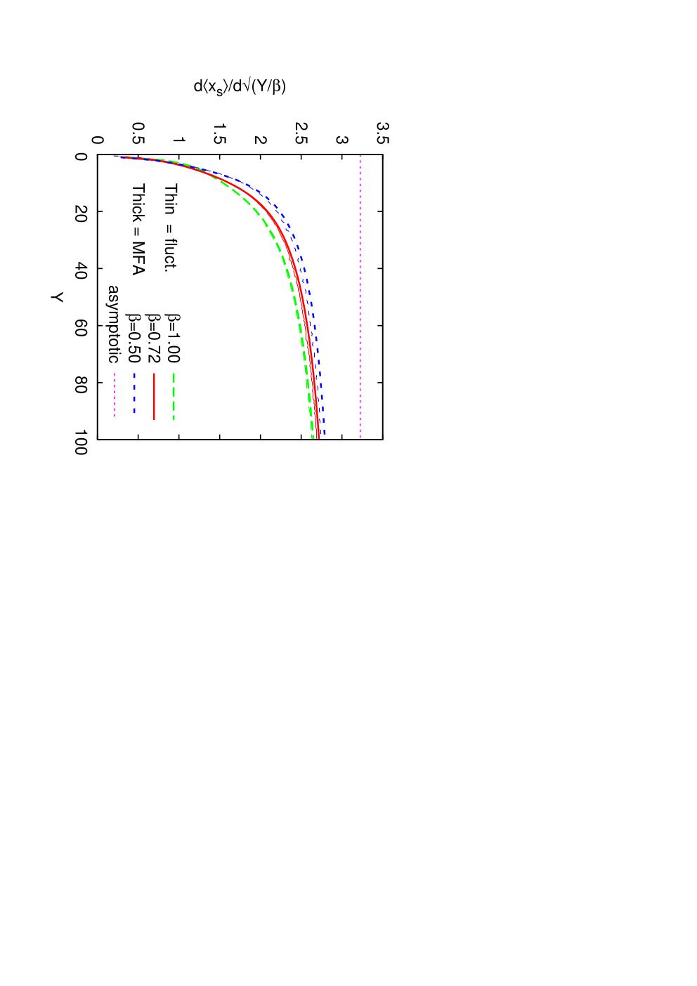
Further evidence for the suppression of fluctuations comes from a study of those quantities which exist already at mean field level, like the (average) position of the front and the corresponding velocity. Our respective numerical results are displayed in Fig. 6, for both the complete evolution and its mean field approximation. These results should be compared to the corresponding ones at FC, in Fig. 1. In the latter, the difference from the mean field behavior is manifest, and is increasing with . In Fig. 6, on the other hand, there are only minor differences between the full evolution and the MFA: the respective curves fall almost on top of each other, for all values of . (The small visible differences are in fact consistent with the magnitude of the dispersion reported in Fig. 3.) In particular, on the right hand figure, one sees that all the velocity curves remain well below the limiting value which is expected at asymptotically large both in the MFA, cf. Eq. (12), and in the full evolution with fluctuations. These results have the following implications:
(a) For the considered range in rapidities, both types of evolution (with or without fluctuations) are still far away from the asymptotic regime.
(b) In the full evolution including fluctuations, the rapidities covered by our simulations are too small for the fronts to be fully formed. (Since, if the fronts were fully formed at some intermediate value of , then their subsequent evolution would have been quite different from the mean field case.) In particular, the fact that the measured front velocity remains significantly smaller than the asymptotic value is not to be attributed to ‘cut–off’ effects due to fluctuations, but rather to preasymptotic effects, which for are the same with or without fluctuations.
Conclusion (b) above can be reformulated by saying that the front ‘formation time’ should be larger than, or marginally comparable to, the maximal rapidity which is covered by our analysis. This is also consistent with the previous results concerning the smallness of fluctuations: as explained in Sect. 3, the fluctuations cannot significantly develop until the individual fronts have been fully formed.
The fact that the front ‘formation time’ can be relatively large at RC should not be a surprise, in view of the discussion in Sect. 3. What is quite surprising, however, is that this quantity can be that large, namely of or even larger. (In fact, in our simulations, we have never seen any sign that the fronts have been formed, until the highest rapidities.) To further consolidate this discovery, we performed another numerical test, which directly measures the front region, and thus the formation time:
(iii) The reduced front: event–by–event geometric scaling
By inspection of the analytic results in Sect. 3 (see, especially, Eqs. (2) and (10) there), one sees that a study of the reduced front can give us access to the width of the geometric scaling window, for both fixed and running coupling. Indeed, for , which includes the saturation region and the transition region around , where the shape of the amplitude is not analytically known, vanishes exponentially, whereas for very large , such that , it rapidly vanishes once again, due to diffusion. On the other hand, within the window for geometric scaling, grows linearly with , cf. Eq. (15); hence, the width of the geometric scaling window can be identified as the region of linear increase for .


We have measured the reduced fronts with both FC and RC, with the results shown in Fig. 7. For fixed coupling (figure on the left), there is a clear difference between the MFA and the complete evolution including fluctuations: whereas in the former case, the scaling window keeps growing with , and quite fast (recall that the respective diffusive radius is expected to grow like , cf. Eq. (3)), in the presence of fluctuations, the growth of the scaling region is similar in the early stages, but then it saturates, around , at a maximal value which defines the width of the front. The fluctuations in the tail of the front at large are clearly visible.
Moving to the RC case (right figure), the situations looks very different: the curves corresponding to mean–field and, respectively, fluctuations are now very close to each other, no fluctuations are visible in the tail, and, besides, the width of the scaling region is much smaller than for FC, as expected (since with RC this region rises only like , cf. Eq. (14)). The fact that, in the fluctuation case, the width of the scaling region keeps growing with confirms that the front has not been formed, in agreement with the previous results in this section. In fact, the maximal extent of the geometric scaling window as seen on this plot is about for , which is rather small — at most, marginally comparable to our previous estimate, Eq. (18), for the front width evaluated for .
(iv) Approximate geometric scaling for the average amplitude
Since our numerical results show very small dispersion, cf. Fig. 3, it is quite clear that the shape of the average amplitude remains close to that of any of the individual fronts which compose the ensemble, and hence to the shape of the mean–field front. We thus expect to exhibit approximate geometric scaling, according to the pattern described below Eq. (10). In order to check this, we have displayed in Fig. 8 the average amplitude emerging from our RC simulations (with ) as a function of the scaling variable , for various values of up to . From this figure, one sees that the various curves fall almost on top of each other for , but they start to deviate from each other for larger values of , although this deviation remains quite small. This behavior is indeed consistent with both the analytic considerations in Sect. 3 and the previous numerical results in this present section. Namely, the value for the upper bound of the geometric scaling window is in agreement with our former results for the reduced front, as shown in the right plot in Fig. 7. Also, the fact that the dispersion between the various curves (at ) is decreasing when increasing , as it can be checked via a close inspection of Fig. 8, is in agreement with our theoretical expectation that the violation of geometric scaling proceeds via BFKL diffusion (cf. Eq. (10)).
The quality of the geometric scaling behavior88 8 This quality could be more precisely characterized with the method proposed in Ref. [42]. visible in Fig. 8 is considerably lower than for the corresponding mean–field results at FC, but much better than it would be for the full FC evolution, including fluctuations. (For , the stochastic FC evolution with would generate a dispersion , which is large enough for the geometric scaling to be completely washed out in the average amplitude, and replaced by diffusive scaling; cf. Fig. 2 and the discussion in Ref. [34].) In fact, the amount of geometric scaling violation in Fig. 8 is indeed comparable to the one observed in the small– data at HERA [40, 41, 42].

We conclude this section with a lesson from our analysis which may shed some light on a rather surprising recent finding in Ref. [32]: namely, in that work, an unexpectedly large ‘anomalous dimension’ was reported, , based on an exponential fit to the fronts generated by the BK equation with running coupling. This value is significantly larger than the saturation anomalous dimension which is expected to control the decay of the amplitude in the geometric scaling region. Or, as we have seen in both Fig. 7 (right figure) and Fig. 8, the window for true scaling is in fact quite narrow: at ; outside this window, the amplitude decays much faster, because of the diffusion term. It is therefore likely that the result reported in Ref. [32] is the consequence of enforcing an exponential fit over a relatively large window in , much larger than the actual window for geometric scaling.
5 Conclusions and outlook
In this paper we have presented the first analysis of the consequences of the running of the coupling on the high–energy evolution with Pomeron loops, in the context of a simple one–dimensional model which captures the relevant dynamics in QCD. We have found that the Pomeron loop effects are strongly suppressed by the running of the coupling, up to the highest energies that we have investigated — which go well beyond the energies of interest for the phenomenology of QCD. The main reason for this surprising behavior is the fact that, in the presence of a running coupling, the diffusive radius grows very slowly with rapidity. Therefore, the wave fronts preserve a pre–asymptotic shape which is not favorable for the growth of fluctuations. During this pre–asymptotic evolution, which in our simulations extends up to , the dynamics is similar to the respective prediction of the mean–field approximation (with running coupling, of course). In particular, due to the suppressed dispersion, approximate geometric scaling is preserved for the average scattering amplitude. The window for strict geometric scaling is rather narrow, but an approximate scaling behavior extends well outside this window. We believe that this should suffice to explain the respective scaling observed in the HERA data, but a firm conclusion in that sense would deserve a dedicated study.
In the course of our analysis, we have performed various numerical tests to verify that our conclusions are insensitive to the details of the numerical procedure (e.g., the discretization of the spatial axis), to the prescription used the ‘freeze’ the running of the coupling in the infrared, and also to the specific implementation of a running coupling in the context of the model (in addition to our main choice, Eq. (6), for the running of , we have also performed calculations with some other prescriptions, and obtained similar results).
It is also useful at this stage to summarize the limitations of our present analysis, and thus pave the way towards further studies: This study has been restricted to asymmetric initial conditions (dilute projectile vs. dense target), where the projectile corresponds to a dipole in QCD. This setup covers those physical problems which, in QCD, admit a dipolar factorization — chiefly among them, deep inelastic scattering, but also particle production at forward rapidities in hadron–hadron (, ) collisions. However, our current model can accommodate arbitrary initial conditions, including more symmetric ones, and it would be interesting to study the influence of the initial conditions on our main conclusion (the suppression of Pomeron loop effects by the running of the coupling). This could shed more light on the physical mechanism responsible for this suppression and, in particular, consolidate the argument about the front formation time that we have proposed, and which seems to be supported by the present analysis.
Furthermore, it would be important to clarify the model–dependence of our conclusions, if any. If the extension of the present analysis to real QCD (which would require solving the Pomeron loop equations of Refs. [8, 10]) looks still prohibitive for the time being, it would be nevertheless interesting to apply a similar study to other one–dimensional models of the ‘reaction–diffusion’ type, and thus check whether the universality expected for such models still persists after the inclusion of running coupling effects. This may have physical consequences for other kinds of problems, say in the framework of statistical physics, where what we call ‘running coupling’ in the context of QCD would actually correspond to an inhomogeneous medium, in which the rates for particle splitting and merging scale with like (powers of) .
Acknowledgments
We would like to thank Al Mueller for fruitful discussions and insightful remarks on our early numerical results. We acknowledge useful discussions with Guillaume Beuf and Robi Peschanski. L.P. would like to acknowledge CAPES for financial support. G.S. is funded by the National Funds for Scientific Research (FRNS, Belgium). This manuscript has been authored under Contract No. DE-AC02-98CH10886 with U.S. Department of Energy.
References
- [1] I. Balitsky, Nucl. Phys. B463 (1996) 99; Phys. Lett. B518 (2001) 235; “High-energy QCD and Wilson lines”, hep-ph/0101042.
- [2] Yu.V. Kovchegov, Phys. Rev. D60 (1999) 034008; ibid. D61 (1999) 074018.
- [3] J. Jalilian-Marian, A. Kovner, A. Leonidov and H. Weigert, Nucl. Phys. B504 (1997) 415; Phys. Rev. D59 (1999) 014014; J. Jalilian-Marian, A. Kovner and H. Weigert, Phys. Rev. D59 (1999) 014015; A. Kovner, J. G. Milhano and H. Weigert, Phys. Rev. D62 (2000) 114005.
- [4] H. Weigert, Nucl. Phys. A703 (2002) 823.
- [5] E. Iancu, A. Leonidov and L. McLerran, Nucl. Phys. A692 (2001) 583; Phys. Lett. B510 (2001) 133; E. Ferreiro, E. Iancu, A. Leonidov and L. McLerran, Nucl. Phys. A703 (2002) 489.
- [6] A.H. Mueller and A.I. Shoshi, Nucl. Phys. B692 (2004) 175.
- [7] E. Iancu, A.H. Mueller and S. Munier, Phys. Lett. B606 (2005) 342.
- [8] E. Iancu and D.N. Triantafyllopoulos, Nucl. Phys. A756 (2005) 419.
- [9] E. Iancu and D.N. Triantafyllopoulos, Phys. Lett. B610 (2005) 253.
- [10] A.H. Mueller, A.I. Shoshi, S.M.H. Wong, Nucl. Phys. B715 (2005) 440.
- [11] E. Levin and M. Lublinsky, Nucl. Phys. A763 (2005) 172.
- [12] A. Kovner and M. Lublinsky, Phys. Rev. Lett. 94 (2005) 181603; Phys. Rev. D71 (2005) 085004.
- [13] Y. Hatta, E. Iancu, L. McLerran, A. Stasto, D.N. Triantafyllopoulos, Nucl. Phys. A764 (2006) 423.
- [14] I. Balitsky, Phys. Rev. D72 (2005) 074027.
- [15] E. Brunet, B. Derrida, A. H. Mueller and S. Munier, Phys. Rev. E73 (2006) 056126 [cond-mat/0512021].
- [16] C. Marquet, R. Peschanski and G. Soyez, Phys. Rev. D73 (2006) 114005.
- [17] Y. Hatta, E. Iancu, C. Marquet, G. Soyez, D.N. Triantafyllopoulos, Nucl. Phys. A773 (2006) 95.
- [18] E. Iancu, C. Marquet, and G. Soyez, Nucl. Phys. A780 (2006) 52.
- [19] M. Kozlov, A.I. Shoshi, B.-W. Xiao, “Total gluon shadowing due to fluctuation effects”, hep-ph/0612053.
- [20] K. Golec-Biernat, L. Motyka, and A.M. Staśto, Phys. Rev. D65 (2002) 074037.
- [21] E. Iancu, K. Itakura, and L. McLerran, Nucl. Phys. A708 (2002) 327.
- [22] A.H. Mueller and D.N. Triantafyllopoulos, Nucl. Phys. B640 (2002) 331.
- [23] D.N. Triantafyllopoulos, Nucl. Phys. B648 (2003) 293.
- [24] S. Munier and R. Peschanski, Phys. Rev. D69 (2004) 034008.
- [25] K. Rummukainen and H. Weigert, Nucl. Phys. A739 (2004) 183.
- [26] E. Iancu, K. Itakura, and D.N. Triantafyllopoulos, Nucl. Phys. A742 (2004) 182.
- [27] J.L. Albacete, N. Armesto, J.G. Milhano, C.A. Salgado and U.A. Wiedemann, Phys. Rev. D71 (2005) 014003.
- [28] E. Gardi, J. Kuokkanen, K. Rummukainen and H. Weigert, Nucl. Phys. A784 (2007) 282.
- [29] Yu.V. Kovchegov and H. Weigert, Nucl. Phys. A784 (2007) 188.
- [30] I. Balitsky, Phys. Rev. D75 (2007) 014001.
- [31] Yu.V. Kovchegov and H. Weigert, Nucl. Phys. A789 (2007) 260.
- [32] J.L. Albacete and Yu.V. Kovchegov, arXiv:0704.0612.
- [33] V.S. Fadin, R. Fiore, A. Papa, Nucl. Phys. B769 (2007) 108; Phys. Lett. B647 (2007) 179.
- [34] E. Iancu, J.T. de Santana Amaral, G. Soyez, and D.N. Triantafyllopoulos, Nucl. Phys. A786 (2007) 131.
- [35]
L.N. Lipatov, Sov. J. Nucl. Phys. 23
(1976) 338;
E.A. Kuraev, L.N. Lipatov and V.S. Fadin, Zh. Eksp. Teor. Fiz 72, 3 (1977) (Sov. Phys. JETP 45 (1977) 199);
Ya.Ya. Balitsky and L.N. Lipatov, Sov. J. Nucl. Phys. 28 (1978) 822. - [36] J.-P. Blaizot, E. Iancu, and D.N. Triantafyllopoulos, Nucl. Phys. A784 (2007) 227.
- [37] For a recent review, see W. Van Saarloos, Phys. Rep. 386 (2003) 29.
- [38] E. Brunet and B. Derrida, Phys. Rev. E56 (1997) 2597; Comp. Phys. Comm. 121-122 (1999) 376; J. Stat. Phys. 103 (2001) 269.
- [39] S. Munier and R. Peschanski, Phys. Rev. Lett. 91 (2003) 232001.
- [40] A.M. Stasto, K. Golec-Biernat and J. Kwiecinski, Phys. Rev. Lett. 86 (2001) 596.
- [41] C. Marquet and L. Schoeffel, Phys. Lett. B639 (2006) 471.
- [42] F. Gelis, R. Pechanski, G. Soyez, and L. Schoeffel, Phys. Lett. B647 (2007) 376.
- [43] J. Bartels, K. Golec-Biernat, and H. Kowalski, Phys. Rev. D66 (2002) 014001.
- [44] E. Iancu, K. Itakura and S. Munier, Phys. Lett. B590 (2004) 199.
- [45] G. Soyez, “Saturation QCD predictions with heavy quarks at HERA”, arXiv:0705.3672.
- [46] A.H. Mueller and G.P. Salam, Nucl. Phys. B475 (1996) 293.
- [47] A.H. Mueller, Nucl. Phys. B415 (1994) 373; ibid. B437 (1995) 107.
- [48] E. Iancu and L. McLerran, Phys. Lett. B510 (2001) 145.
- [49] C. Marquet, G. Soyez, and Bo-Wen Xiao, Phys. Lett. B639 (2006) 635.
- [50] L.V. Gribov, E.M. Levin, and M.G. Ryskin, Phys. Rept. 100 (1983) 1.