Matching polytopes, toric geometry, and the totally non-negative GrassmannianThanks: Alexander Postnikov was supported in part by NSF CAREER Award DMS-0504629. David Speyer was supported by a research fellowship from the Clay Mathematics Institute. Lauren Williams was supported in part by the NSF
Abstract.
In this paper we use toric geometry to investigate the topology of the totally non-negative part of the Grassmannian, denoted . This is a cell complex whose cells can be parameterized in terms of the combinatorics of plane-bipartite graphs . To each cell we associate a certain polytope . The polytopes are analogous to the well-known Birkhoff polytopes, and we describe their face lattices in terms of matchings and unions of matchings of . We also demonstrate a close connection between the polytopes and matroid polytopes. We use the data of to define an associated toric variety . We use our technology to prove that the cell decomposition of is a CW complex, and furthermore, that the Euler characteristic of the closure of each cell of is .
Key words and phrases:
Total positivity, Grassmannian, CW complexes, Birkhoff polytope, matching, matroid polytope, cluster algebra2000 Mathematics Subject Classification
Primary 05Exx; Secondary 20G20, 14Pxx1. Introduction
The classical theory of total positivity concerns matrices in which all minors are non-negative. While this theory was pioneered by Gantmacher, Krein, and Schoenberg in the 1930’s, the past decade has seen a flurry of research in this area initiated by Lusztig [9, 10, 11]. Motivated by surprising connections he discovered between his theory of canonical bases for quantum groups and the theory of total positivity, Lusztig extended this subject by introducing the totally non-negative variety in an arbitrary reductive group and the totally non-negative part of a real flag variety .
Recently Postnikov [13] investigated the combinatorics of the totally non-negative part of a Grassmannian : he established a relationship between and certain planar bicolored graphs, producing a combinatorially explicit cell decomposition of . To each such graph he constructed a parameterization of a corresponding cell of by . In fact, this cell decomposition is a special case of a cell decomposition of which was conjectured by Lusztig and proved by Rietsch [15], although that cell decomposition was described in quite different terms. Other combinatorial aspects of , and more generally of , were investigated by Marsh and Rietsch [12], Rietsch [16], and the third author [22, 23].
It is known that is contractible [9] and it is conjectured that with its cell decomposition is a regular CW complex homeomorphic to a ball. In [23], the third author proved the combinatorial analogue of this conjecture, proving that the partially ordered set (poset) of cells of is in fact the poset of cells of a regular CW complex homeomorphic to a ball.
In this paper we give an approach to this conjecture which uses toric geometry to extend to a map onto the closure of the corresponding cell of . Specifically, given a plane-bipartite graph , we construct a toric variety and a rational map . We show that is well-defined on the totally non-negative part of and that its image is the closure of the corresponding cell of . The totally non-negative part of is homeomorphic to a certain polytope (the moment polytope) which we denote , so we can equally well think of this result as a parameterization of our cell by . The restriction of to the toric interior of the non-negative part of (equivalently, to the interior of ) is .
Our technology proves that the cell decomposition of the totally non-negative part of the Grassmannian is in fact a CW complex. While our map is well-defined on (which is a closed ball) and is a homeomorphism on the interior, in general is not a homeomorphism on the boundary of ; therefore this does not lead directly to a proof of the conjecture. However, we do obtain more evidence that the conjecture is true: using Williams’ result [23] that the face poset of is Eulerian, it follows that the Euler characteristic of the closure of each cell of is .
The most elegant part of our story is how the combinatorics of the plane-bipartite graph reflects the structure of the polytope and hence the structure of . See Table 1 for some of these connections. The torus fixed points of correspond to perfect orientations of , equivalently, to almost perfect matchings of . The other faces of correspond to certain elementary subgraphs of , that is, to unions of almost perfect matchings of . Every face of is of the form for some plane-bipartite graph obtained by deleting some edges of , and restricted to is . It will follow from this that, for every face of , the interior of is mapped to the interior of a cell of the totally non-negative Grassmannian with fibers that are simply affine spaces. We hope that this explicit description of the topology of the parameterization will be useful in studying the topology of .
| Plane-Bipartite graph | Polytope |
|---|---|
| Dimension of | |
| Perfect orientations / almost perfect matchings | Vertices of |
| Equivalence classes of edges | Facets of |
| Lattice of elementary subgraphs | Lattice of faces of |
The structure of this paper is as follows. In Section 2 we review the combinatorics of plane-bipartite graphs and perfect orientations. Next, in Section 3 we review toric varieties and their non-negative parts, and prove a lemma which is key to our CW complex result. We then, in Section 4, introduce the polytopes which will give rise to the toric varieties of interest to us. Using these polytopes, in Section 5 we make the connection between our polytopes and matroid polytopes and explain the relation of our results to problems arising in cluster algebras and tropical geometry. In Section 6 we use these polytopes to prove that the cell decomposition of is in fact a CW complex. In Section 7 we analyze the combinatorics of our polytopes in greater detail, giving a combinatorial description of the face lattice of in terms of matchings and unions of matchings of . Finally, in Section 8, we calculate -vectors, Ehrhart series, volumes, and the degrees of the corresponding toric varieties for a few small plane-bipartite graphs.
Acknowledgements: We are grateful to Vic Reiner for pointing out the similarity between our polytopes and Birkhoff polytopes, and to Allen Knutson for many helpful conversations.
2. The totally non-negative Grassmannian and plane-bipartite graphs
In this section we review some material from [13]. We have slightly modified the notation from [13] to make it more convenient for the present paper.
Recall that the (real) Grassmannian is the space of all -dimensional subspaces of , for . An element of can be viewed as a full-rank matrix modulo left multiplications by nonsingular matrices. In other words, two matrices represent the same point in if and only if they can be obtained from each other by row operations.
Let be the set of all -element subsets of . For , let denote the maximal minor of a matrix located in the column set . The map , where ranges over , induces the Plücker embedding .
Definition 2.1.
[13, Section 3] The totally non-negative Grassmannian is the subset of the real Grassmannian that can be represented by matrices with all maximal minors non-negative.
For , the positive Grassmann cell is the subset of the elements in represented by all matrices with the prescribed collection of maximal minors strictly positive , for , and the remaining maximal minors equal to zero , for .
A subset such that is nonempty satifies the base axioms of matroid. These special matroids are called positroids.
Clearly is a disjoint union of the positive Grassmann cells . It was shown in [13] that each of these cells is really a cell, that is, it is homeomorphic to an open ball of appropriate dimension . Moreover, one can explicitly construct a parametrization using certain planar graphs, as follows.
Definition 2.2.
A plane-bipartite graph is an undirected graph drawn inside a disk (considered modulo homotopy) with boundary vertices on the boundary of the disk, labeled in clockwise order, as well as some colored internal vertices. These internal vertices are strictly inside the disk and are colored in black and white such that:
- (1)
Each edge in joins two vertices of different colors.
- (2)
Each boundary vertex in is incident to a single edge.
A perfect orientation of a plane-bipartite graph is a choice of directions of its edges such that each black internal vertex is incident to exactly one edge directed away from ; and each white internal vertex is incident to exactly one edge directed towards . A plane-bipartite graph is called perfectly orientable if it has a perfect orientation. Let denote the directed graph associated with a perfect orientation of . The source set of a perfect orientation is the set of for which is a source of the directed graph . Similarly, if , then is a sink of .
All perfect orientations of a fixed have source sets of the same size where . Here the sum is over all internal vertices , for a black vertex , and for a white vertex; see [13]. In this case we say that is of type .
Let us associate a variable with each edge of . Pick a perfect orientation of . For and , define the boundary measurement as the following power series in the :
where the sum is over all directed paths in that start at the boundary vertex and end at the boundary vertex . The Laurent monomial is given by , where the product is over all edges in directed from a white vertex to a black vertex, and the product is over all edges in directed from a black vertex to a white vertex. For any path , let ,, …, be the directions of the edges of (in order). Let be the path through which travels from to to and so forth, traveling less then units of arc from each to the next. The winding index is the number of times winds around the circle , rounded to the nearest integer. The index is congruent to the number of self-intersections of the path modulo .
Remark 2.3.
Let us mention several differences in the notations given above and the ones from [13]. The construction in [13] was done for plabic graphs, which are slightly more general than the plane-bipartite graphs defined above. Edges in plabic graphs are allowed to join vertices of the same color. One can easily transform a plabic graph into a plane-biparte graph, without much change in the construction, by contracting edges which join vertices of the same color, or alternatively, by inserting vertices of different color in the middle of such edges.
Another difference is that we inverted the edge variables from [13] for all edges directed from a black vertex to a white vertex.
In [13] the boundary measurements were defined for any planar directed graph drawn inside a disk. It was shown that one can easily transform any such graph into a plane-bipartite graph with a perfect orientation of edges that has the same boundary measurements.
Let denote the edge set of a plane-bipartite graph , and let denote the set of vectors with strictly positive real coordinates .
Lemma 2.4.
[13, Lemma 4.3] The sum in each boundary measurement evaluates to a subtraction-free rational expression in the . Thus it gives a well-defined positive function on .
For example, suppose that has two boundary vertices, and and two internal vertices and , with edges , , and running connecting , , and . Then . The sum only converges when but, by interpreting it as a rational function, we can see that it gives a well defined value for any -tuple of positive reals.
If the graph is acyclic then there are finitely many directed paths , and for any . In this case the are clearly Laurent polynomials in the with positive integer coefficients, and the above lemma is trivial.
For a plane-biparte graph of type and a perfect orientation with the source set , let us construct the matrix such that
- (1)
The submatrix of in the column set is the identity matrix.
- (2)
For any and , the minor equals .
These conditions uniquely define the matrix . Its entries outside the column set are . The matrix represents an element of the Grassmannian . Thus, by Lemma 2.4, it gives the well-defined boundary measurement map
Clearly, the matrix described above will be different for different perfect orientations of . However, all these different matrices represent the same point in the Grassmannian .
Note that once we have constructed the matrix , we can determine which cell of we are in by simply noting which maximal minors are nonzero and which are zero.
Proposition 2.5.
[13, Theorem 10.1] For a perfectly orientable plane-bipartite graph , the boundary measurement map does not depend on a choice of perfect orientation of .
If we multiply the edge variables for all edges incident to an internal vertex by the same factor, then the boundary measurement will not change. Let denote the set of internal vertices of . Let be the quotient of modulo the action of given by these rescalings of the . If the graph does not have isolated connected components without boundary vertices11 1 Clearly, we can remove all such isolated components without affecting the boundary measurements., then . The map induces the map
which (slightly abusing the notation) we also call the boundary measurement map.
Talaska [21] has given an explicit combinatorial formula for the maximal minors (also called Plücker coordinates) of such matrices . To state her result, we need a few definitions. A conservative flow in a perfect orientation of is a (possibly empty) collection of pairwise vertex-disjoint oriented cycles. (Each cycle is self-avoiding, i.e. it is not allowed to pass through a vertex more than once.) For , a flow from to is a collection of self-avoiding walks and cycles, all pairwise vertex-disjoint, such that the sources of these walks are and the destinations are . So a conservative flow can also be described as a flow from to . The weight of a flow is the product of the weights of all its edges directed from the white to the black vertex, divided by the product of all its edges directed from the black to the white vertex.22 2 Note that here we slightly differ from Talaska’s convention in order to be consistent with our previous convention in defining . A flow with no edges has weight .
Theorem 2.6.
[21, Theorem 1.1] Fix a perfectly orientable and a perfect orientation . The minor of , with columns in position , is given by
Here the sum in the numerator is over flows from to and the sum in the denominator is over all conservative flows .
A point in the Grassmannian only depends on its Plücker coordinates up to multiplication by a common scalar. For our purposes, it is best to clear the denominators in Theorem 2.6, and give a purely (Laurent) polynomial formula:
Corollary 2.7.
Using the notation of Theorem 2.6, the point of corresponding to the row span of has Plücker coordinates
where the sum is over flows from to .
Theorem 2.6 implies that the image of the boundary measurement map lies in the totally non-negative Grassmannian . Moreover, the image is equal to a certain positive cell in .
Proposition 2.8.
[13, Theorem 12.7] Let be any perfectly orientable plane-bipartite graph of type . Then the image of the boundary measurement map is a certain positive Grassmann cell in . For every cell in , there is a perfectly orientable plane-bipartie graph such that is the image of . The map is a fiber bundle with fiber an -dimensional affine space, for some non-negative . For any cell of , we can always choose a graph such that is a homeomorphism onto this cell.
Let us say that a plane-bipartite graph is reduced if is a homeomorphism, and has no isolated connected components nor internal vertices incident to a single edge; see [13].
An almost perfect matching of a plane-bipartite graph is a subset of edges such that each internal vertex is incident to exactly one edge in (and the boundary vertices are incident to either one or no edges in ). There is a bijection between perfect orientations of and almost perfect matchings of where, for a perfect orientation of , an edge is included in the corresponding matching if is directed away from a black vertex or to a white vertex in .33 3 Note that typically is directed away from a black vertex if and only if it is directed towards a white vertex. However, we have used the word or to make the bijection well-defined when boundary vertices are not colored.
For a plane-bipartite graph and the corresponding cell in , one can combinatorially construct the matroid from the graph , as follows.
Proposition 2.9.
[13, Propostion 11.7, Lemma 11.10] A subset is a base of the matroid if and only there exists a perfect orientation of such that .
Equivalently, assuming that all boundary vertices in are black, is a base of if and only if there exists an almost perfect matching of such that
3. Toric varieties and their non-negative parts
We may define a (generalized) projective toric variety as follows [2, 19]. Let be any finite subset of , where can be thought of as the character group of the torus . Here . Then consider the map such that . Here denotes . We then define the toric variety to be the Zariski closure of the image of this map. We write for the inclusion of into The real part of is defined to be the intersection of with ; the positive part is defined to be the image of under ; and the non-negative part is defined to be the closure of in . We note for future reference that , and are unaltered by translating the set by any integer vector.
Note that is not necessarily a toric variety in the sense of [5], as it may not be normal; however, its normalization is a toric variety in that sense. See [2] for more details.
Let be the convex hull of . There is a homeomorphism from to , known as the moment map. (See [5, Section 4.2, page 81] and [19, Theorem 8.4]). In particular, is homeomorphic to a closed ball.
We now prove a simple but very important lemma.
Lemma 3.1.
Suppose we have a map given by
where the ’s are Laurent polynomials with positive coefficients. Let be the set of all exponent vectors in which occur among the (Laurent) monomials of the ’s, and let be the convex hull of the points of . Then the map factors through the totally positive part , giving a map . Moreover extends continuously to the closure to give a well-defined map .
Proof.
Let . Clearly the map factors as the composite map , and the image of under the first map is precisely . The second map, which we will call , takes a point of to , where the ’s are homogeneous polynomials of degree with positive coefficients. By construction, each occurs in at least one of the ’s.
Since is the closure inside of , any point of has all ’s non-negative; furthermore, not all of the ’s are equal to . And now since the ’s have positive coefficients and they involve all of the ’s, the image of any point of under is well-defined. Therefore extends continuously to the closure to give a well-defined map .
∎
In Section 6 we will use this lemma to prove that is a CW complex.
4. Matching polytopes for plane-bipartite graphs
In this section we will define a family of polytopes associated to plane-bipartite graphs .
Definition 4.1.
Given an almost perfect matching of a plane-bipartite graph , we associate to it the 0-1 vector in where the coordinates associated to edges in the matching are and all other coordinates are . We define to be the convex hull of these - vectors.
Remark 4.2.
Note that more generally, we could define for any graph with a distinguished subset of “boundary” vertices. Many of our forthcoming results about for plane-bipartite graphs should be extendable to this generality.
Because all of the - vectors above have the property that for all internal vertices of , the polytope lies in the subspace of defined by .
We will now see how one can arrive at these polytopes in another way. Recall that for each we have the boundary measurement map . Embedding the image into projective space via the Plücker embedding, we have an explicit formula for the coordinates given by Talaska (Corollary 2.7).
In the following definition, we use the notation of Theorem 2.6.
Definition 4.3.
Fix a perfect orientation of . We define to be the convex hull of the exponent vectors of the weights of all flows starting at . A priori this polytope lies in , but we will see that lies in a subspace of .
Remark 4.4.
We now relate and . We continue to use the notion of flows introduced in shortly before Theorem 2.6.
Lemma 4.5.
Fix a plane-bipartite graph and a perfect orientation . If we choose a flow in and switch the direction of all edges in this flow, we obtain another perfect orientation. Conversely, one can obtain any perfect orientation of from by switching all directions of edges in a flow in .
Proof.
The first claim is simple: a perfect orientation is one in which each black vertex has a unique outcoming edge and each white vertex has a unique incoming edge. If we switch the orientation of all edges along one of the paths or cycles in the flow, clearly this property will be preserved.
To see the converse, let denote the set of edges of in which the orientations and disagree. It follows from the definition of perfect orientation that every edge in incident to some vertex can be paired uniquely with another edge in which is also incident to (note that at each vertex of there are either or incident edges which are in ). This pairing induces a decomposition of into a union of vertex-disjoint (undirected) cycles and paths. Moreover, each such cycle or path is directed in both and (but of course in opposite directions). This set of cycles and paths is the relevant flow. ∎
Because of the bijection between perfect orientations and almost perfect matchings (see Section 2), Lemma 4.5 implies the following.
Corollary 4.6.
Fix and a perfect orientation . Flows in are in bijection with perfect orientations of (obtained by reversing all edges of the flow in ) which are in bijection with almost perfect matchings of .
We can now see the following.
Corollary 4.7.
For any perfect orientation , the polytope is a translation of by an integer vector.
Proof.
Let denote the empty flow on , be some other flow in , and the perfect orientation obtained from by reversing the directions of all edges in . Let and be the almost perfect matchings associated to and . Let , , , and be the vectors in associated to this flow and these perfect orientations. Of course is the all-zero vector. We claim that .
Fix an edge of : we will check that the -coordinates of and are equal. First, suppose that does not occur in . Then either appears in both and , or in neither. So and either or . Now, suppose that occurs in , and is oriented from its white to its black endpoint in . So and . The edge occurs in the matching and not in the matching , so and . Finally, suppose occurs in , and is oriented from its black to its white endpoint in . Then and . The edge occurs in the matching and not in the matching , so and . ∎
In particular, up to translation, does not depend on . Recall that translating a polytope does not affect the corresponding toric variety.
In Figure 1, we fix a plane-bipartite graph corresponding to the cell of such that the Plücker coordinates are positive and all others are . We display the three perfect orientations and the vertices of .

In Figure 2, we fix a plane-bipartite graph corresponding to the cell of such that the Plücker coordinates are positive while and are . We display the four perfect orientations and the vertices of .

In Figure 3 we have fixed a plane-bipartite graph corresponding to the top-dimensional cell of . has seven perfect orientations. We have drawn the edge graph of the four-dimensional polytope . This time we have depicted the vertices of using matchings instead of perfect orientations. Next to each matching, we have also listed the source set of the corresponding perfect orientation.

5. Connections with matroid polytopes and cluster algebras
Every perfectly orientable plane-bipartite graph encodes a realizable positroid, that is, an oriented matroid in which all orientations are positive. The bases of the positroid associated to a plane-bipartite graph of type are precisely the -element subsets which occur as source sets of perfect orientations of . This is easy to see, as each perfect orientation of gives rise to a parametrization of the cell of in which the Plücker coordinate corresponding to the source set is . Furthermore, if one takes a (directed) path in a perfect orientation and switches the orientation of each of its edges, this encodes a basis exchange.
Given this close connection of perfectly orientable plane-bipartite graphs to positroids, it is natural to ask whether there is a connection between our polytopes and matroid polytopes. We first recall the definition of a matroid polytope. Let be a matroid of rank on the ground set . The matroid polytope is the convex hull of the vectors where is the vector in whose th coordinate is if and is otherwise [7]. The vertices are in one-to-one correspondence with bases of . This polytope lies in the hyperplane and, if the matroid is connected, has dimension .
Proposition 5.1.
There is a linear projection from to . The fibers of this projection over the vertices of are the Newton polytopes for the Laurent polynomials which express the Plücker coordinates on in terms of the edge variables.
Proof.
If is a plane-bipartite graph of type , one can associate to each vertex of the basis of the corresponding positroid corresponding to the boundary edges which are matched in . In terms of the bijection between perfect matchings and perfect orientations, this is the source set of the corresponding perfect orientation. This gives the linear projection from to . To see that the statement about the fibers is true, see Corollary 2.7, and remember the relationship between matchings and flows. ∎
The second and third authors, in [20], related the Newton polytopes of Proposition 5.1 to the positive part of the tropical Grassmannian; our results in that paper can be summarized by saying that the positive part of the tropical Grassmannian is combinatorially isomorphic to the dual fan of the fiber polytope of the map . 44 4 We worked with face variables rather than edge variables in [20], but the two corresponding realizations of are linearly isomorphic.
The fact that the Plücker coordinates on can all be expressed as Laurent polynomials in the edge weights is not simply a fortunate coincidence, but is a consequence55 5 This consequence is not completely straightforward; one must express certain ratios of the edge weights as Laurent monomials in the variables of a certain cluster, and this involves a nontrivial “chamber Ansatz”. of the fact that the coordinate ring of has the structure of a cluster algebra. (See [4] for the definition of cluster algebras, [17] for the verification that the largest cell of the Grassmannian has the structure of a cluster algebra and [13] for the fact that every has this structure.) In general, if we had a better understanding of the Newton polytopes of Laurent polynomials arising from cluster algebras, we could resolve many of the open questions in that theory.
Example 5.2.
Consider the plane-bipartite graph from Figure 3. This corresponds to the positroid of rank two on the ground set such that all subsets of size are independent. The edge graph of the four-dimensional polytope is shown in Figure 3, and each vertex is labeled with the basis it corresponds to. The matroid polytope of this matroid is the (three-dimensional) octahedron with six vertices corresponding to the two-element subsets of . Under the map , each vertex of corresponding to the two-element subset gets mapped to the vertex of the octahedron whose th and th coordinates are (all other coordinates being ).
6. is a CW complex
We now prove that the cell decomposition of is a CW complex, and obtain as a corollary that the Euler characteristic of the closure of each cell is .
To review the terminology, a cell complex is a decomposition of a space into a disjoint union of cells, that is open balls. A CW complex is a cell complex together with the extra data of attaching maps. More specifically, each cell in a CW complex is attached by gluing a closed -dimensional ball to the -skeleton , i.e. the union of all lower dimensional cells. The gluing is specified by a continuous function from to . CW complexes are defined inductively as follows: Given a discrete space (a discrete union of -cells), and inductively constructed subspaces obtained from by attaching some collection of -cells, the resulting colimit space is called a CW complex provided it is given the weak topology and every closed cell is covered by a finite union of open cells.
Although we don’t need this definition here, we note that a regular CW complex is a CW complex such that the closure of each cell is homeomorphic to a closed ball and the boundary of each cell is homeomorphic to a sphere. It is not known if the cell decomposition of is regular, although the results of [23] suggest that the answer is yes.
Lemma 6.1.
Theorem 6.2.
The cell decomposition of is a finite CW complex.
Proof.
All of these cell complexes contain only finitely many cells; therefore the closure-finite condition in the definition of a CW complex is automatically satisfied. What we need to do is define the attaching maps for the cells: we need to prove that for each -dimensional cell there is a continuous map from to which maps to and extends the parameterization of the cell (a map from the interior of to ).
By Corollary 2.7, if we are given a perfectly orientable plane-bipartite graph , the image of the parameterization of the cell under the Plücker embedding can be described as a map to projective space, where the ’s are Laurent polynomials with positive coefficients. By Lemma 3.1 and Remark 4.4, the map gives rise to a rational map which is well-defined on (a closed ball). Furthermore, it is clear that the image of on lies in .
Since the totally positive part of the toric variety is dense in the non-negative part, and the interior gets mapped to the cell , it follows that gets mapped to the closure of . Furthermore, by construction, maps homeomorphically to the cell .
And now by Lemma 6.1, it follows that the boundary of gets mapped to the -skeleton of . This completes the proof that the cell decomposition of is a CW complex. ∎
It has been conjectured that the cell decomposition of is a regular CW complex which is homeomorphic to a ball. In particular, if a CW complex is regular then it follows that the Euler characteristic of the closure of each cell is .
In [23], the third author proved that the poset of cells of is thin and lexicographically shellable, hence in particular, Eulerian. In other words, the Mobius function of the poset of cells takes values for any in the poset. As the Euler characteristic of a finite CW complex is defined to be the number of even-dimensional cells minus the number of odd-dimensional cells, we obtain the following result.
Corollary 6.3.
The Euler characteristic of the closure of each cell of is .
7. The face lattice of
We now consider the lattice of faces of , and give a description in terms of unions of matchings of . This description is very similar to the description of the face lattice of the Birkhoff polytopes, as described by Billera and Sarangarajan [1]. In fact our proofs are very similar to those in [1]; we just need to adapt the proofs of Billera and Sarangarajan to the setting of plane-bipartite graphs.
We begin by giving an inequality description of the polytope .
Proposition 7.1.
For any plane bipartite graph , the polytope is given by the following inequalities and equations: for all edges , and for each internal vertex . If every edge of is used in some almost perfect matching, then the affine linear space defined by the above equations is the affine linear space spanned by .
Proof.
Let be the polytope defined by these inequalities. Clearly, is contained in . Note that lies in the cube because if is any edge of and an endpoint of then everywhere on we have . Let be a vertex of . We want to show that is a -vector. Suppose for the sake of contradiction that is not a -vector; let be the subgraph of consisting of edges for which . Note that, if is a vertex of , then has degree at least in since . Therefore, contains a cycle or a path from one boundary vertex of to another. We consider the case where contains a cycle, the other case is similar. Let , , …, be the edges of this cycle; the length of the cycle is even because is bipartite. Define the vector by and if . Let . Then and are both in , contradicting that was assumed to be a vertex of .
Now, assume that every edge of is used in some almost perfect matching. Then meets the interior of the orthant , so the affine linear space spanned by is the same as the affine linear space which cuts it out of this orthant. ∎
Corollary 7.2.
Suppose that every edge of is used in some almost perfect matching. Then has dimension .
Proof.
By proposition 7.1, the affine linear space spanned by is parallel to the vector space cut out by the equations . This is precisely , where is the set of boundary vertices of . Let be the graph formed from by identifying the vertices of . We embed in a sphere by contracting the boundary of the disc in which lives to a point. Then , which has dimension . ∎
Note that Corollary 7.2 is correct even when some components of are not connected to the boundary, in which case some of the faces of are not discs.
7.1. The lattice of elementary subgraphs
Following [8], we call a subgraph of elementary if it contains every vertex of and if every edge of is used in some almost perfect matching of . Equivalently, the edges of are obtained by taking a union of several almost perfect matchings of . (To see the equivalence, if , then each edge of occurs in some , which is an almost perfect matching of . Conversely, if is elementary, then let , , …, be the almost perfect matchings of contained in then, by the definition of “elementary”, .)
The main result of this section is the following.
Theorem 7.3.
The face lattice of is isomorphic to the lattice of all elementary subgraphs of , ordered by inclusion.
Proof.
We give the following maps between faces of and elementary subgraphs. If is a face of , let be the set of edges of such that is not identically zero on , and let be the subgraph of with edge set . Since is a face of a -polytope, is the convex hull of the characteristic vectors of some set of matchings, and is the union of these matchings. Thus, is a map from faces of to elementary subgraphs. Conversely, if is a subgraph of , let . Since defines a face of , the intersection is a face of . From the description in Proposition 7.1, every face of is of the form for some subgraph of . Note also that .
We need to show that these constructions give mutually inverse bijections between the faces of and the elementary subgraphs. For any face of , it is clear that . Suppose for the sake of contradiction that . Then is contained in some proper face of ; let this proper face be for some . Then there is an edge of which is not in . By the condition that is in , the function cannot be zero on , so is not contained in after all. We deduce that .
Conversely, let be an elementary subgraph of . It is clear that . Suppose for the sake of contradiction that there is an edge of which is not in . Since is elementary, there is a matching of which contains the edge . Let be the corresponding vertex of . Then is not zero on , so is in after all and we conclude that . ∎
The minimal nonempty elementary subgraphs of are the matchings, corresponding to vertices of .
Corollary 7.4.
Consider a cell of parameterized by a plane-bipartite graph . For any cell in the closure of , the corresponding polytope is a face of .
7.2. Facets and further combinatorial structure of
We now give a description of the facets of . Let us say that two edges and of are equivalent if they separate the same pair of (distinct) faces and with the same orientation. That is, if we travel across from face to , the black vertex of will be to our left if and only if when we travel across from to , the black vertex of is to our left.
Lemma 7.5.
If every edge of is used in an almost perfect matching then two edges and are equivalent if and only if the linear functionals and have the same restriction to .
Proof.
By Proposition 7.1, the affine linear space spanned by is cut out by the equations , where runs through the internal vertices of . Let be the linear space cut out by the equations ; the polytope is parallel to and thus the functionals and have the same restriction to if and only if they have the same restriction to . In the proof of Corollary 7.2 we identified with . So we just want to determine when the restrictions of and to are the same.
The restrictions of and to are elements of the dual vector space . We can identify with the vector space of functions on summing to zero as follows: Map to by sending an edge to the function which is on one of the faces it borders and on the other; the sign convention is that the sign is positive or negative according to whether lies to the right or left of , when is oriented from black to white. Then , which is defined as a quotient of , is the image of this map.
We now see that and restrict to the same functional on if and only if they correspond to the same function on the faces of . This occurs if and only if they separate the same pair of faces with the same orientation. ∎
Theorem 7.6.
Suppose that is elementary. Then the facets of correspond to the elementary subgraphs of the form , where is an equivalence class as above.
Proof.
First, note that if and are not equivalent then, by Lemma 7.5, and have different restrictions to . Thus, there is no facet of on which they both vanish. On the other hand, if and are equivalent then, again by Lemma 7.5, on every facet of where vanishes, also vanishes. So we see that every facet of is of the form , where is an equivalence class in . (Here is the function introduced in the proof of Theorem 7.3.)
If is a facet of then is elementary, by Theorem 7.3. Conversely, if is elementary then is a face of . Since all the edges of separate the same pair of faces, has one less face than , so is a facet of , as desired. ∎
As a special case of the preceding propositions, we get the following.
Remark 7.7.
Let be a face of and let be the number of regions into which the edges of divide the disk in which is embedded. Then is an edge of if and only if . Equivalently, two vertices and of form an edge if and only if can be obtained from by switching the orientation along a self-avoiding path or cycle in .
Recall that the Birkhoff polytope is the convex hull of the points in where is equal to if and is equal to otherwise. It is well-known that is an dimensional polytope, whose face lattice of is isomorphic to the lattice of all elementary subgraphs of the complete bipartite graph ordered by inclusion [1]. Our polytopes can be thought of as analogues of the Birkhoff polytope for planar graphs embedded in a disk.
8. Appendix: numerology of the polytopes
In this section we give some statistics about a few of the polytopes . Our computations were made with the help of the software polymake [6].
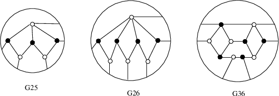
Let denote the plane-bipartite graph from Figure 3, and let , , and denote the plane-bipartite graphs shown in Figures 4. These plane-bipartite graphs give parameterizations of the top cells in , and , respectively.
The -vectors of the matching polytopes , , and are , , , and respectively. The Ehrhart series for , and , which give the Hilbert series of the corresponding toric varieties, are , , and . The volumes of the four polytopes are , , , and . Thus, the degrees of the corresponding toric varieties are , , , and .
Proposition 8.1.
Let (for ) be the family of graphs that extend the first two graphs shown in Figure 4. Then the number of vertices of is given by .
Proof.
This can be proved by induction on by removing the leftmost black vertex. We leave this as an exercise for the reader. ∎
Note that in general there is more than one plane-bipartite graph giving a parameterization of a given cell. But even if two plane-bipartite graphs and correspond to the same cell, in general we have . For example, the plane-bipartite graph in Figure 5 gives a parameterization of the top cell of . Let us refer to this graph as . However, : the -vector of is .

References
- [1] L. Billera, A. Sarangarajan, the Combinatorics of permutation polytopes, DIMACS Series in Discrete Mathematics and Theoretical Computer Science 24, 1996.
- [2] D. Cox, What is a toric variety? Topics in algebraic geometry and geometric modeling, 203–223, Contemp. math., 334, Amer. Math. Soc., Providence, RI, 2003.
- [3] S. Fomin, M. Shapiro, Stratified spaces formed by totally positive varieties, Mich. Math. J. 48 (2000), 253–270.
- [4] S. Fomin, A. Zelevinsky, Cluster Algebras I: Foundations, J. Amer. Math. Soc. 22 (2002), 497–527.
- [5] W. Fulton, Introduction to toric varieties, Annals of Mathematics Studies, 131, Princeton University Press, Princeton, NY, 1993.
- [6] E. Gawrilow, M. Joswig, polymake: a framework for analyzing convex polytopes and simplicial complexes. http://www.math.tu-berlin.de/polymake, 1997–2003. Version 2.0, with contributions by Thilo Schroder and Nikolaus Witte.
- [7] I. Gelfand, R. Goresky, R. MacPherson, V. Serganova, Combinatorial geometries, convex polyhedra, and Schubert cells, Adv. in Math. 63 (1987), no. 3, 301–316.
- [8] L. Lovasz, M. Plummer, Matching Theory, Elsevier Science Pub. Co. New York, 1986.
- [9] G. Lusztig, Introduction to total positivity, in Positivity in Lie theory: open problems, ed. J. Hilgert, J.D. Lawson, K.H. Neeb, E.B. Vinberg, de Gruyter Berlin, 1998, 133–145.
- [10] G. Lusztig, Total positivity in partial flag manifolds, Representation Theory, 2 (1998) 70–78.
- [11] G. Lusztig, Total positivity in reductive groups, in: Lie theory and geometry: in honor of Bertram Kostant, Progress in Mathematics 123, Birkhauser, 1994.
- [12] R. Marsh, K. Rietsch, Parametrizations of flag varieties, Representation Theory, 8 (2004).
- [13] A. Postnikov, Total positivity, Grassmannians, and networks. http://front.math.ucdavis.edu/math.CO/0609764
- [14] J. Propp, Lattice Structure for Orientations of Graphs, preprint. http://front.math.ucdavis.edu/math.CO/0209005
- [15] K. Rietsch, Total positivity and real flag varieties, Ph.D. Dissertation, MIT, 1998.
- [16] K. Rietsch, Closure relations for totally non-negative cells in , Math. Res. Lett. 13 (2006), no. 5-6, 775–786.
- [17] J. Scott, Grassmannians and cluster algebras, Proceedings of the London Math. Soc. (3) 92, 2006, no. 2, 345 – 380.
- [18] A. Schrijver, Theory of linear and integer programming, Wiley-Interscience series in discrete mathematics and optimization, John Wiley and Sons, New York, 1986.
- [19] F. Sottile, Toric ideals, real toric varieties, and the moment map, in Topics in Algebraic Geometry and Geometric Modeling, Contemp. Math. 334, 2003, 225 – 240.
- [20] D. Speyer and L. Williams, The tropical totally positive Grassmannian, J. Algebraic Combin. 22 (2005), no. 2, 189–210.
- [21] K. Talaska, A formula for Plücker coordinates of a perfectly oriented network, to appear in Internat. Math. Res. Not. arXiv:0801.4822
- [22] L. Williams, Enumeration of totally positive Grassmann cells, Adv. Math., 190 (2), 2005, 319–342.
- [23] L. Williams, Shelling totally non-negative flag varieties, J. Reine Angew. Math. (Crelle’s Journal), 609, 2007, 1–22.
- [24] G. Ziegler, Lectures on Polytopes, Graduate Texts in Mathematics, 152, Springer-Verlag, New York, 1995.