Multiple inflation and the WMAP ‘glitches’
II. Data analysis and cosmological parameter extraction

Paul Hunt^1,2 and Subir Sarkar¹ Affiliation: ¹ Rudolf Peierls Centre for Theoretical Physics, University of Oxford, 1 Keble Road, Oxford OX1 3NP, UK
² Institute of Theoretical Physics, Warsaw University, ul Hoża 69, 00-681 Warsaw, POLAND

Abstract

Detailed analyses of the WMAP data indicate possible oscillatory features in the primordial curvature perturbation, which moreover appears to be suppressed beyond the present Hubble radius. Such deviations from the usual inflationary expectation of an approximately Harrison-Zeldovich spectrum are expected in the supergravity-based ‘multiple inflation’ model wherein phase transitions during inflation induce sudden changes in the mass of the inflaton, thus interrupting its slow-roll. In a previous paper we calculated the resulting curvature perturbation and showed how the oscillations arise. Here we perform a Markov Chain Monte Carlo fitting exercise using the 3-year WMAP data to determine how the fitted cosmological parameters vary when such a primordial spectrum is used as an input, rather than the usually assumed power-law spectrum. The ‘concordance’ $\Lambda$ CDM model is still a good fit when there is just a ‘step’ in the spectrum. However if there is a ‘bump’ in the spectrum (due e.g. to two phase transitions in rapid succession), the precision CMB data can be well-fitted by a flat Einstein-de Sitter cosmology without dark energy. This however requires the Hubble constant to be $h\simeq 0.44$ which is lower than the locally measured value. To fit the SDSS data on the power spectrum of galaxy clustering requires a $\sim 10\%$ component of hot dark matter, as would naturally be provided by 3 species of neutrinos of mass $\sim 0.5$ eV. This CHDM model cannot however fit the position of the baryon acoustic peak in the LRG redshift two-point correlation function. It may be possible to overcome these difficulties in an inhomogeneous Lemaître-Tolman-Bondi cosmological model with a local void, which can potentially also account for the SN Ia Hubble diagram without invoking cosmic acceleration.

pacs

98.80.Cq, 98.70.Vc

I Introduction

Precision measurements of CMB anisotropies by the Wilkinson Microwave Anisotropy Probe (WMAP) are widely accepted to have firmly established the ‘concordance’ $\Lambda$ CDM model — a flat universe with $\Omega_{\Lambda}\simeq 0.7$ , $\Omega_{\mathrm{m}}\simeq 0.3$ , $h\simeq 0.7$ , seeded by a nearly scale-invariant power-law spectrum of adiabatic density fluctuations Spergel:2003cb; Spergel:2006hy. However the model fit to the data is surprisingly poor. For the WMAP-1 TT spectrum, $\chi_{\rm eff}^{2}/\nu=974/893$ Spergel:2003cb, so formally the $\Lambda$ CDM model is ruled out at $97\%$ c.l. Visually the most striking discrepancies are at low multipoles where the lack of power in the Sachs-Wolfe plateau and the absence of the expected $\Lambda$ -induced late integrated-Sachs-Wolfe effect have drawn much attention. However because cosmic variance and uncertainties in the foreground subtraction are high on such scales, it has been argued that the observed low quadrupole (and octupole) are not particularly unlikely, see e.g. refs.Efstathiou:2003wr; Slosar:2004xj; Park:2006dv. The excess $\chi^{2}$ in fact originates mainly from sharp features or ‘glitches’ in the power spectrum that the model is unable to fit Spergel:2003cb; Hinshaw:2006ia. Although these glitches are less pronounced in the 3-year data release, they are still present Hinshaw:2006ia. Hence although the fit to the concordance $\Lambda$ CDM model has improved with $\chi_{\rm eff}^{2}/\nu=1049/982$ for the WMAP-3 TT spectrum Spergel:2006hy, this model still has only a 6.8% chance of being a correct description of the data. This is less than reassuring given the significance of such a tiny cosmological constant (more generally, ‘dark energy’) for both cosmology and fundamental physics.

The WMAP team state: “In the absence of an established theoretical framework in which to interpret these glitches (beyond the Gaussian, random phase paradigm), they will likely remain curiosities” Hinshaw:2006ia. However it had been noted earlier by the WMAP team themselves Peiris:2003ff that these may correspond to sharp features in the spectrum of the underlying primordial curvature perturbation, arising due to sudden changes in the mass of the inflaton in the ‘multiple inflation’ model proposed in ref.Adams:1997de. This generates characteristic localized oscillations in the spectrum, as was demonstrated numerically in a toy model of a ‘chaotic’ inflationary potential having a ‘step’ starting at $\phi_{\mathrm{step}}$ with amplitude and gradient determined by the parameters $c_{\mathrm{ampl}}$ and $d_{\mathrm{grad}}$ : $V(\phi)=\frac{1}{2}m_{\phi}^{2}\phi^{2}\left[1+c_{\mathrm{ampl}}\tanh\left(\frac{\phi-\phi_{\mathrm{step}}}{d_{\mathrm{grad}}}\right)\right]$ Adams:2001vc. It was found that the fit to the WMAP-1 data improves significantly (by $\Delta\chi^{2}=10$ ) for the model parameters $\phi_{\mathrm{step}}=15.5\,M_{\mathrm{P}}$ , $c_{\mathrm{ampl}}=9.1\times 10^{-4}$ and $d_{\mathrm{grad}}=1.4\times 10^{-2}\,M_{\mathrm{P}}$ , where $M_{\mathrm{P}}\equiv(8\pi\,G_{\mathrm{N}})^{-1/2}\simeq 2.44\times 10^{18}$ GeV Peiris:2003ff. However the cosmological model parameters were held fixed (at their concordance model values) in this exercise. Recently this analysis has been revisited using the WMAP-3 data Covi:2006ci; these authors also consider departures from the concordance model and conclude that there are virtually no degeneracies of cosmological parameters with the modelling of the spectral feature Hamann:2007pa.

However $m$ in the toy model above is not the mass of the inflaton — in fact in all such chaotic inflation models with $V\propto\phi^{n}$ where inflation occurs at field values $\phi_{\mathrm{infl}}>M_{\mathrm{P}}$ , the leading term in a Taylor expansion of the potential around $\phi_{\mathrm{infl}}$ is always linear since this is not a point of symmetry German:2001tz. The effect of a change in the inflaton mass in multiple inflation can be sensibly modelled only in a ‘new’ inflation model where inflation occurs at field values $\phi<<M_{\rm Pl}$ and an effective field theory description of the inflaton potential is possible. The ‘slow-roll’ conditions are violated when the inflaton mass changes suddenly due to its (gravitational) coupling to ‘flat direction’ fields which undergo thermal phase transitions as the universe cools during inflation Adams:1997de. The resulting effect on the spectrum of the curvature perturbation was found by analytic solution of the governing equations to correspond to an upward step followed by rapidly damped oscillations Hunt:2004vt.¹¹ 1 A ‘hybrid’ inflation model wherein the inflaton is coupled to a ‘curvaton’ field also yields oscillations together with suppressed power on large scales Langlois:2004px. A similar phenomenon had been noted earlier for the case where the inflaton potential has a jump in its slope Starobinsky:ts; however such a discontinuity has no physical interpretation. The WMAP glitches have also been interpreted as due to the effects of ‘trans-Planckian’ physics Martin:2003sg; Danielsson:2006gg; Spergel:2006hy and due to resonant particle production Mathews:2004vu.

One can ask if spectral features are seen when one attempts to recover the primordial perturbation spectrum directly from the data. Such attempts may be divided into two classes. Usually the curvature perturbation, $\mathcal{P_{R}}(k)$ , is given a simple parameterisation and fitted to the data, together with the background cosmology, using MCMC likelihood analysis. The spectrum has been described using bins in wave number $k$ Bridle:2003sa; Hannestad:2003zs; Bridges:2005br; Bridges:2006zm, wavelets Mukherjee:2003ag, smoothing splines Sealfon:2005em and principal components Leach:2005av. However for MCMC analysis to be feasible, the number of parameters must be limited, so the reconstructed spectrum has too low a resolution to reveal anything interesting. By contrast, ‘non-parametric’ methods assume the background cosmology (usually the concordance $\Lambda$ CDM model) so that the transfer function is known, and then invert the data to find the primordial perturbation spectrum. Methods that have been used are the Richardson-Lucy deconvolution algorithm Shafieloo:2003gf; Shafieloo:2006hs, an iterative, semi-analytic process Kogo:2003yb; Kogo:2004vt, and a smoothed, least-squares procedure Tocchini-Valentini:2004ht; Tocchini-Valentini:2005ja. The perturbation spectra produced by the first and third methods have a prominent step followed by bumps which are rather reminiscent of decaying oscillations (see Fig.4 in ref.Hunt:2004vt). These features correspond in fact to the depressed quadrupole and the glitches at low multipole $\ell$ .

Encouraged by this we consider possible variations of the primordial perturbation spectrum beyond the limited set considered so far, and motivated by the multiple inflation model. We have shown earlier that a phase transition in a ‘flat direction’ field during inflation (in a supergravity framework) generates a step in the primordial spectrum followed by damped oscillations Hunt:2004vt. In a physical supergravity model there are many such flat directions and these will undergo phase transitions in rapid succession after the first $\sim 10-15$ e-folds of inflation (assuming they all start from the origin due e.g. to thermal initial conditions) Adams:1997de. Hence we also consider a possible ‘bump’ in the spectrum due to two phase transitions in rapid succession, which raise and then lower the inflaton mass. We wish to emphasise that there may well be other physical frameworks wherein one can expect similar features in the primordial spectrum. Our intention here is to use a definite and calculable framework, in order to illustrate how the extraction of cosmological parameters is dependent on the assumed form of the primordial spectrum. We find that the precision WMAP data can be fitted just as well without invoking dark energy if there is indeed a bump in the primordial spectrum around the position of the first acoustic peak in the angular power spectrum of the CMB. To fit the position of the first peak (assuming a flat model as motivated by inflation) requires however a low Hubble constant, $h\sim 0.44$ , in contrast to the value of $h=0.72\pm 0.08$ measured by the Hubble Key Project (HKP) in our local neighbourhood Freedman:2000cf. Although a pure CDM model is well known to suffer from excess power on small scales, data from the Sloane Digital Sky Survey (SDSS) on galaxy clustering Tegmark:2003uf can also be well fitted if there is a $\sim 10\%$ component of hot dark matter, as has been noted already using the 2dFGRS data Elgaroy:2003yh; Blanchard:2003du. This is encouraging given the evidence for neutrino mass from oscillations, and the required value of $\sim 0.5$ eV per species is well within the present experimental upper bound of 2.3 eV Yao:2006px. Such a cold + hot dark matter (CHDM) model with a low Hubble constant passes all the usual cosmological tests (e.g. cluster baryon fraction and $\sigma_{8}$ from clusters and weak lensing Blanchard:2003du) but has difficulty Blanchard:2005ev matching the position of the ‘baryon acoustic oscillation’ (BAO) peak observed in the redshift two-point correlation function of luminous red galaxies (LRG) in SDSS Eisenstein:2005su. We confirm that this is indeed the case but wish to draw attention to the possibility that this difficulty may be solved in an inhomogeneous Lemaître-Tolman-Bondi (LTB) cosmological model wherein we are located in an underdense void which is expanding faster than the global rate Biswas:2006ub. Such a model may also account for the SN Ia Hubble diagram without invoking cosmic acceleration Goodwin:1999ej; Celerier:1999hp; Tomita:2000jj; Alnes:2005rw; Enqvist:2006cg; Alnes:2006uk; Celerier:2007jc.

II Multiple Inflation

In previous work we have discussed the effective potential during inflation driven by a scalar field in $N=1$ supergravity, which has couplings to other flat direction fields having gauge and/or Yukawa couplings Adams:1997de. These fields acquire a potential due to supersymmetry breaking by the large vacuum energy driving inflation and evolve rapidly to their minima, which are fixed by the non-renormalisable terms which lift their potential at large field values. The inflaton’s own mass thus jumps as these fields suddenly acquire large vacuum expectation values (vevs), after having been trapped at the origin through their coupling to the thermal background for the first $\sim 10-15$ e-folds of inflation. Damped oscillations are also induced in the inflaton mass as the coupled fields oscillate in their minima losing energy mainly due to the rapid inflationary expansion. The resulting curvature perturbation was calculated in our previous work Hunt:2004vt and will be used in this paper as an input for cosmological parameter extraction using the WMAP-3 data.

In order to produce observable effects in the CMB or large-scale structure the phase transition(s) must take place as cosmologically relevant scales ‘exit the horizon’ during inflation. There are many flat directions which can potentially undergo symmetry breaking during inflation, so it is not unlikely that several phase transitions occurred in the $\sim 8$ e-folds which is sampled by observations Adams:1997de. The observation that the curvature perturbation appears to cut off above the scale of the present Hubble radius suggests that (this last period of) inflation may not have lasted much longer than the minimum necessary to generate an universe as big as the present Hubble volume. Whereas this raises a ‘naturalness’ issue, it is consistent given this state of affairs to consider the possibility that thermal phase transitions in flat direction fields $\sim 10-15$ e-folds after the beginning of inflation leave their mark in the observed scalar density perturbation on the microwave sky and in the large-scale distribution of galaxies.

II.1 ‘Step’ model

The potential for the inflaton $\phi$ and flat direction field $\psi$ (with mass $m$ and $\mu$ respectively) is similar to that given previously Hunt:2004vt:

V(\phi,\psi)=\left\{\begin{array}[]{lc}V_{0}-\frac{1}{2}m^{2}\phi^{2},&t<t_{1},\\ V_{0}-\frac{1}{2}m^{2}\phi^{2}-\frac{1}{2}\mu^{2}\psi^{2}+\frac{1}{2}\lambda\phi^{2}\psi^{2}+\frac{\gamma}{M_{\mathrm{P}}^{n-4}}\psi^{n},&t\geq t_{1}.\end{array}\right.

(1)

Here $t_{1}$ is the time at which the phase transition starts (at $t<t_{1}$ , $\psi$ is trapped at the origin by thermal effects), $\lambda$ is the coupling between the $\phi$ and $\psi$ fields, and $\gamma$ is the co-efficient of the leading non-renormalisable operator of order $n$ which lifts the potential of the flat direction field $\psi$ (and is determined by the nature of the new physics beyond the effective field theory description). Note that the quartic coupling above is generated by a term $\kappa\phi\phi^{\dagger}\psi^{2}/M_{\mathrm{P}}^{2}$ in the Kähler potential with $\kappa\sim 1$ (allowed by symmetry near $\phi\sim 0$ ), so $\lambda=\kappa\,H^{2}/M_{\mathrm{P}}^{2}$ Adams:1997de. We have not considered non-renormalisable operators $\propto\phi^{n}/M_{\mathrm{P}}^{n-4}$ German:2001tz since we are concerned here with the first $\sim 10-20$ e-folds of inflation when $\phi$ is still close to the origin so such operators are then unimportant for its evolution. We are also not addressing here the usual ‘ $\eta$ -problem’ in supergravity models, namely that $m\sim H$ due to supersymmetry breaking by the vacuum energy driving inflation. We assume that some mechanism suppresses this mass to enable sufficient inflation to occur Randall:1997kx; Lyth:1998xn. However this will not be the case in general for the flat direction fields, so one would naturally expect $\mu\sim H$ .

Then the change in the inflaton mass-squared after the phase transition is

\delta m_{\phi}^{2}=\lambda\Sigma^{2},\quad\Sigma=\left[\frac{M_{\mathrm{P}}^{n-4}}{n\gamma}\left(\mu^{2}-\lambda\phi^{2}\right)\right]^{1/\left(n-2\right)}\simeq\left(\frac{\mu^{2}M_{\mathrm{P}}^{n-4}}{n\gamma}\right)^{1/\left(n-2\right)},

(2)

where $\Sigma$ is the vev of the global minimum to which $\psi$ evolves during inflation. The equations of motion are

	$\displaystyle\ddot{\phi}+3H\dot{\phi}=$	$\displaystyle-\frac{\partial V}{\partial\phi}$	$\displaystyle=\left(m^{2}-\lambda\psi^{2}\right)\phi,$		(3)
	$\displaystyle\ddot{\psi}+3H\dot{\psi}=$	$\displaystyle-\frac{\partial V}{\partial\psi}$	$\displaystyle=\left(\mu^{2}-\lambda\phi^{2}-\frac{n\gamma}{M_{\mathrm{P}}^{n-4}}\psi^{n-2}\right)\psi.$		(4)

To characterise the comoving curvature perturbation $\mathcal{R}$ Mukhanov:1990me, we employ the gauge-invariant quantity $u=-z\mathcal{R}$ , where $z=a\dot{\phi}/H$ , $a$ is the cosmological scale-factor and $H$ is the Hubble parameter during inflation. The Fourier components of $u$ satisfy the Klein-Gordon equation of motion: $u^{\prime\prime}_{k}+(k^{2}-z^{\prime\prime}/z)u_{k}=0$ , where the primes indicate derivatives with respect to conformal time $\eta=\int{\rm d}t/a=-1/aH$ (the last equality holds in de Sitter space). For convenience, we use the variable $w_{k}\equiv\sqrt{2k}u_{k}$ , for which this equation reads:

w^{\prime\prime}_{k}+w^{\prime}_{k}+\left[\widetilde{k}^{2}\exp\left(-2\widetilde{t}\right)-2-\widetilde{m}^{2}+\widetilde{\lambda}\widetilde{\psi}^{2}-\frac{2\widetilde{\lambda}\widetilde{\psi}\widetilde{\psi}^{\prime}\widetilde{\phi}}{\widetilde{\phi}^{\prime}}\right]w_{k}=0.

(5)

where we have used the dimensionless variables: $\widetilde{t}=Ht$ , $\widetilde{\phi}=\phi/M_{\mathrm{P}}$ , $\widetilde{\psi}=\psi/M_{\mathrm{P}}$ , $\widetilde{m}=m/H$ , $\widetilde{\lambda}=\lambda M_{\mathrm{P}}^{2}/H^{2}$ and $\widetilde{k}=k/K_{0}$ , where $K_{0}=a_{0}H$ and $a=a_{0}\exp(\widetilde{t})$ . We also define $\widetilde{H}=H/M_{\mathrm{P}}$ and $\widetilde{\mu}=\mu/H$ for convenience. Note that now (and henceforth) the dashes refer to derivatives with respect to $\widetilde{t}$ .

We start the integration at an initial value of the scale-factor $a_{0}$ , which is taken to be several e-folds of inflation before the phase transition occurs. Similarly we choose an initial value $\phi_{0}$ for the inflaton field corresponding to several e-folds of inflation before the phase transition occurs (the precise value does not affect our results).

We use two parameters to characterise the primordial perturbation spectrum. The first is the amplitude of the spectrum on large scales in the slow-roll approximation:

\mathcal{P_{R}}^{(0)}=\left(\frac{H^{2}}{2\pi\dot{\phi}_{0}}\right)^{2}=\frac{9\widetilde{H}^{2}}{4\pi^{2}\widetilde{m}^{4}\widetilde{\phi}_{0}^{2}}.

(6)

The second is $k_{1}\equiv cK_{0}$ where $c$ is a constant chosen so that $k_{1}$ is the position of the step in the spectrum. This can be done because a mode with wavenumber $k$ ‘exits the horizon’ when the coefficient of $w_{k}$ in eq.(5) is zero, hence the wavenumber $k^{\prime}_{1}$ of the mode that exits at the start of the phase transition is

\displaystyle k^{\prime}_{1}\equiv

\displaystyle K_{0}\widetilde{k^{\prime}}_{1}

\displaystyle=K_{0}\sqrt{2+\widetilde{m}^{2}}\ \mathrm{e}^{\widetilde{t}_{1}},

(7)

where $\widetilde{t}_{1}$ is just the number of e-folds of inflation after which the phase transition occurs. Since we keep $\widetilde{m}^{2}$ and $\widetilde{t}_{1}$ fixed, we have $k^{\prime}_{1}\propto K_{0}$ . For the phase transition to significantly influence the primordial perturbation spectrum after the mode with $k=k^{\prime}_{1}$ exits the horizon requires several further e-folds of inflation, depending on how fast the flat direction evolves. The exponential growth of $\widetilde{\psi}$ is governed by the value of $\widetilde{\mu}$ , which we also keep fixed. Therefore the position of the step in the spectrum is proportional to $k_{0}$ . We repeat our analysis for integer values of $n$ , the order of the non-renormalisable term in the effective field theory description, in the range $12$ to $17$ . We set $\widetilde{\lambda}=\gamma=1$ , $\widetilde{m}^{2}=0.005$ , $\widetilde{\phi}_{0}=0.01$ and $\widetilde{\mu}^{2}=3$ . The fractional change in the inflaton mass-squared due to the phase transition is

\Delta m^{2}\equiv\frac{\lambda\Sigma^{2}}{m^{2}}=\frac{\widetilde{\lambda}}{\widetilde{m}^{2}}\left(\frac{\widetilde{\mu}^{2}\widetilde{H}^{2}}{n\gamma}\right)^{\frac{2}{n-2}}.

(8)

Thus fixing the value of $n$ does not entirely fix $\Delta m^{2}$ , because from eq.(6) varying $P_{\mathcal{R}}^{(0)}$ also alters $\widetilde{H}$ . A typical value is $P_{\mathcal{R}}^{(0)}\sim 10^{-9}$ so the corresponding Hubble parameter is $H\sim 3\times 10^{-8}M_{\mathrm{P}}$ i.e. an inflationary energy scale of $\sim 2\times 10^{14}$ GeV. This is comfortably within the upper limit of $\sim 2\times 10^{16}$ GeV set by the WMAP bound on inflationary gravitational waves Kinney:2006qm. Indeed the gravitational wave background is completely negligible for the ‘new’ inflation potential we consider, with the tensor to scalar ratio expected to be: $r\sim\widetilde{m}^{4}\widetilde{\phi}^{2}\sim 10^{-9}$ .

We varied four parameters describing the homogeneous background cosmology which is taken to be a spatially flat Friedman-Robertson-Walker (FRW) universe: the physical baryon density $\omega_{\mathrm{b}}\equiv\Omega_{\mathrm{b}}h^{2}$ , the physical cold dark matter density $\omega_{\mathrm{c}}\equiv\Omega_{\mathrm{c}}h^{2}$ , the ratio $\theta$ of the sound horizon to the angular diameter distance (multiplied by 100), and the optical depth $\tau$ (due to reionisation) to the last scattering surface. The dark energy density is given by $\Omega_{\Lambda}=1-\Omega_{\mathrm{m}}$ , where $\Omega_{\mathrm{m}}\equiv\Omega_{\rm c}+\Omega_{\rm b}$ .

II.2 ‘Bump’ model

Next we consider a multiple inflation model with two successive phase transitions caused by 2 flat direction fields, $\psi_{1}$ and $\psi_{2}$ . The potential is now:

V\left(\phi,\psi_{1},\psi_{2}\right)=\left\{\begin{array}[]{ll}V_{0}-\frac{1}{2}m^{2}\phi^{2},&t<t_{1},\\ V_{0}-\frac{1}{2}m^{2}\phi^{2}-\frac{1}{2}\mu_{1}^{2}\psi_{1}^{2}+\frac{1}{2}\lambda_{1}\phi^{2}\psi_{1}^{2}+\frac{\gamma_{1}}{M_{\mathrm{P}}^{n_{1}-4}}\psi^{n_{1}},&t_{2}\geq t\geq t_{1},\\ V_{0}-\frac{1}{2}m^{2}\phi^{2}-\frac{1}{2}\mu_{1}^{2}\psi_{1}^{2}+\frac{1}{2}\lambda_{1}\phi^{2}\psi_{1}^{2}+\frac{\gamma_{1}}{M_{P}^{n_{1}-4}}\psi^{n_{1}}\\ -\frac{1}{2}\mu_{2}^{2}\psi_{2}^{2}-\frac{1}{2}\lambda_{2}\phi^{2}\psi_{2}^{2}+\frac{\gamma_{2}}{M_{\mathrm{P}}^{n_{2}-4}}\psi^{n_{2}},&t\geq t_{2},\end{array}\right.

(9)

where $t_{1}$ and $t_{2}$ are the times at which the first and second phase transitions occur. After $t_{2}$ , for example, the equations of motion are

$\displaystyle\ddot{\phi}+3H\dot{\phi}=$	$\displaystyle-\frac{\partial V}{\partial\phi}$	$\displaystyle=\left(m^{2}-\lambda_{1}\psi_{1}^{2}+\lambda_{2}\psi_{2}^{2}\right)\phi,$	(10)
$\displaystyle\ddot{\psi_{1}}+3H\dot{\psi_{1}}=$	$\displaystyle-\frac{\partial V}{\partial\psi_{1}}$	$\displaystyle=\left(\mu_{1}^{2}-\lambda_{1}\phi^{2}-\frac{n_{1}\gamma_{1}}{M_{\mathrm{P}}^{n_{1}-4}}\psi_{1}^{n_{1}-2}\right)\psi_{1},$	(11)
$\displaystyle\ddot{\psi_{2}}+3H\dot{\psi_{2}}=$	$\displaystyle-\frac{\partial V}{\partial\psi_{2}}$	$\displaystyle=\left(\mu_{2}^{2}+\lambda_{2}\phi^{2}-\frac{n_{2}\gamma_{2}}{M_{\mathrm{P}}^{n_{2}-4}}\psi_{2}^{n_{2}-2}\right)\psi_{2},$	(12)

and

\frac{1}{z}\frac{d^{2}z}{d\eta^{2}}=a^{2}\left(2H^{2}+m^{2}-\lambda_{1}\psi_{1}^{2}+\lambda_{2}\psi_{2}^{2}-\frac{2\lambda_{1}\psi_{1}\dot{\psi_{1}}\phi}{\dot{\phi}}+\frac{2\lambda_{2}\psi_{2}\dot{\psi_{2}}\phi}{\dot{\phi}}\right).

(13)

The inflaton mass $m_{\phi}$ thus changes due to the phase transitions as

m^{2}\rightarrow m^{2}-\lambda_{1}\Sigma_{1}^{2}\rightarrow m^{2}-\lambda_{1}\Sigma_{1}^{2}+\lambda_{2}\Sigma_{2}^{2}.

(14)

By choosing $\lambda_{2}$ to be of opposite sign to $\lambda_{1}$ (possible in the supergravity model), a bump is thus generated in $\mathcal{P_{R}}$ . In the slow-roll approximation the amplitude of the primordial perturbation spectrum first increases from $\mathcal{P_{R}}^{(0)}$ to $\mathcal{P_{R}}^{(1)}$ then falls to $\mathcal{P_{R}}^{(2)}$ , moving from low to high wavenumbers, where

\mathcal{P_{R}}^{(0)}=\frac{9\widetilde{H}^{2}}{4\pi^{2}\widetilde{m}^{4}\widetilde{\phi}_{0}^{2}},\qquad\mathcal{P_{R}}^{(1)}=\frac{\mathcal{P}_{\mathcal{R}}^{\left(0\right)}}{\left(1-\Delta m_{1}^{2}\right)^{2}},\qquad\mathcal{P_{R}}^{(2)}=\frac{\mathcal{P_{R}}^{(0)}}{\left(1-\Delta m_{1}^{2}+\Delta m_{2}^{2}\right)^{2}}\ .

(15)

We calculate the curvature perturbation spectrum for this model in a way similar to that for the model with one phase transition. As before we specify the homogeneous background cosmology using $\omega_{\rm b}$ , $\theta$ and $\tau$ and, anticipating the discussion later, the fraction of dark matter in the form of neutrinos $f_{\nu}\equiv\Omega_{\nu}/\Omega_{\rm d}$ where the total dark matter density is $\Omega_{\rm d}\equiv\Omega_{\rm c}+\Omega_{\nu}$ . The primordial perturbation spectrum is parameterised in a similar way to that of the first model using $\mathcal{P_{R}}^{(0)}$ and $k_{1}\equiv cK_{0}$ , which is now the approximate position of the first step in the spectrum. A measure of the position of the second step is given by the third parameter

k_{2}\equiv k_{1}\mathrm{e}^{(\widetilde{t}_{2}-\widetilde{t}_{1})},

(16)

where the exponent is just the number of Hubble times after the beginning of the first phase transition when the second one starts. Initially we examined models with $n_{1}=12$ and $n_{2}=13$ , and then we let $\mathcal{P_{R}}^{(1)}$ and $\mathcal{P_{R}}^{(2)}$ vary freely. We set $\widetilde{\lambda}_{1}$ , $\widetilde{\lambda}_{2}$ , $\gamma_{1}$ and $\gamma_{2}$ all equal to unity, $\widetilde{m}^{2}=0.005$ , $\widetilde{\phi}_{0}=0.01$ and $\widetilde{\mu}_{1}^{2}=\widetilde{\mu}_{2}^{2}=3$ throughout.

III The Data Sets

We fit to the WMAP 3-year Hinshaw:2006ia temperature-temperature (TT), temperature-electric polarisation (TE), and electric-electric polarisation (EE) spectra alone as we wish to avoid possible systematic problems associated with combining other CMB data sets. We also fit the linear matter power spectrum $\mathcal{P}_{\mathrm{m}}(k)$ to the SDSS measurement of the real space galaxy power spectrum $\mathcal{P}_{\mathrm{g}}(k)$ Tegmark:2003uf. The two spectra are taken to be related through a scale-independent bias factor $b_{\rm SDSS}$ so that $\mathcal{P}_{\mathrm{m}}(k)=b_{\rm SDSS}^{2}\mathcal{P}_{\mathrm{g}}(k)$ . This bias is expected to be close to unity and we analytically marginalise over it using a flat prior.

We also fit our models to the redshift two-point correlation function of the SDSS LRG sample, which was obtained assuming a fiducial cosmological model with $\Omega_{\mathrm{m}}=0.3$ , $\Omega_{\Lambda}=0.7$ and $h=0.7$ Eisenstein:2005su. The correlation function is dependent on the choice of background cosmology so we rescale it appropriately as explained below, in order to confront it with the other cosmological models we consider. Again we consider a linear bias $b_{\mathrm{LRG}}$ , and determine it from the fit itself.

Parameter	Lower limit	Upper limit
$\omega_{\mathrm{b}}$	$0.005$	$0.1$
$\omega_{\mathrm{c}}$	$0.01$	$0.99$
$\theta$	$0.5$	$10.0$
$\tau$	$0.01$	$0.8$
$\ln\left(10^{10}\mathcal{P_{R}}^{(0)}\right)$	$0.01$	$6.0$
$10^{4}k_{1}/\mathrm{Mpc}^{-1}$	$0.01$	$600.0$
$b_{\mathrm{LRG}}$	$1.0$	$4.0$
$h$	$0.4$	$1.0$
Age/Gyr	$10.0$	$20.0$

Table 1: The priors adopted on the input parameters of the step model, as well as on the derived parameters: the Hubble constant and the age of the Universe.

Parameter	Lower limit	Upper limit
$\omega_{\mathrm{b}}$	$0.005$	$0.1$
$\theta$	$0.5$	$10.0$
$\tau$	$0.01$	$0.8$
$f_{\nu}$	$0.01$	$0.3$
$\ln\left(10^{10}\mathcal{P_{R}}^{(0)}\right)$	$0.01$	$6.0$
$b_{\mathrm{LRG}}$	$1.0$	$4.0$
$h$	$0.1$	$1.0$
Age/Gyr	$10.0$	$20.0$

Table 2: The priors adopted on the input parameters of the bump model with

n_{1}=12

n_{1}=13

, as well as on the derived parameters: the Hubble constant and the age of the Universe. The priors set on the position of the steps are given in Table 3.

	WMAP	+SDSS	+LRG	+SDSS+LRG
$10^{4}k_{1}/\mathrm{Mpc}^{-1}$	$600.0$	$600.0$	$600.0$	$600.0$
$10^{4}k_{2}/\mathrm{Mpc}^{-1}$	$1100.0$	$1100.0$	$600.0$	$600.0$

Table 3: The prior upper limits set for the position of the steps in the spectrum for the ‘bump’ model. In each case the lower limit is

10^{-6}\,\mathrm{Mpc}^{-1}

III.1 WMAP

To date the most accurate observations of the CMB angular power spectra, both TT and TE, have been made by the WMAP satellite using 20 differential radiometers arranged in 10 ‘differencing assemblies’ at 5 different frequency bands between 23 and 94 GHz. Each differencing assembly produces a statistically independent stream of time-ordered data. Full sky maps were generated from the calibrated data using iterative algorithms. The use of different frequency channels enable astrophysical foreground signals to be removed and the angular power spectra were calculated using both ‘pseudo- $C_{\ell}$ ’ and maximum likelihood based methods Hinshaw:2006ia. We use the 3-year data release of the TT, TE and EE spectra and also the code for calculating the likelihood (incorporating the covariance matrix), made publicly available by the WMAP team.²² 2 http://lambda.gsfc.nasa.gov/

Our special interest is in the fact that apart from the quadrupole there are several other multipoles for which the binned power lies outside the 1 $\sigma$ cosmic variance error. These are associated with small, sharp features in the TT spectrum termed glitches, e.g. at $\ell$ = 22, 40 and 120 in both the 1-year and 3-year data release. The pseudo- $C_{\ell}$ method produces correlated estimates for neighbouring $C_{\ell}$ ’s which means it is difficult to judge the goodness-of-fit of a model by eye. The contribution to the $\chi^{2}$ per multipole for the best fit $\Lambda$ CDM model is shown in Fig.17 of ref.Hinshaw:2006ia, where it is apparent that the excess $\chi^{2}$ originates largely from the multipoles at $\ell\lesssim 120$ .

III.2 SDSS

The Sloan Digital Sky Survey (SDSS) consists of a 5 band imaging survey and a spectroscopic survey covering a large fraction of the sky, carried out together using a 2.5 m wide-field telescope. For the spectroscopic survey targets are chosen from the imaging survey to produce three catalogues: the main galaxy sample, the luminous, red galaxy (LRG) sample and the quasar sample, which extend out to redshifts of $z\sim 0.3$ , 0.5 and 5 respectively. The matter power spectrum (up to a multiplicative bias factor $b_{\mathrm{SDSS}}$ ) has been measured using about $2\times 10^{5}$ galaxies which form the majority of the main galaxy sample from the second SDSS Data Release Tegmark:2003uf. After correcting for redshift-space distortion due to galaxy peculiar velocities, the galaxy density field was expanded in terms of Karhunen-Loeve eigenmodes (which is more convenient than a Fourier expansion for surveys with complex geometries) and the power spectrum was estimated using a quadratic estimator. We fit to the 19 k-band measurements in the range $0.01<k<0.2\,h\,\mathrm{Mpc^{-1}}$ , as the fluctuations turn non-linear on smaller scales.

III.3 LRG

The large effective volume of the SDSS LRG sample allowed an unambiguous detection of the BAO peak in the two-point correlation function of galaxy clustering Eisenstein:2005su. The redshifts of $5\times 10^{4}$ LRG’s were translated into comoving coordinates assuming a fiducial $\Omega_{\Lambda}=0.7,\Omega_{\mathrm{m}}=0.3$ cosmology. The correlation function was then found using the Land-Szalay estimator. This can be rescaled for other cosmological models as follows.

An object at redshift $z$ with an angular size of $\Delta\theta$ and extending over a redshift interval $\Delta z$ has dimensions in redshift space $x_{\|}$ and $x_{\bot}$ , parallel and perpendicular to the line-of-sight, given by

x_{\|}=\frac{\Delta z}{H\left(z\right)},\quad x_{\bot}=\left(1+z\right)D_{A}\left(z\right)\Delta\theta.

(17)

Thus the volume in redshift space is $\propto D_{\mathrm{A}}^{2}(z)/H(z)$ , where $D_{\mathrm{A}}$ is the angular diameter distance. The distances between galaxies in redshift space, hence the scale of features in the redshift correlation function, are proportional to the cube root of the volume occupied by the galaxies in redshift space. Therefore the multiplicative rescaling factor between the scale of the BAO peak in the fiducial model and that in another model is just:

\gamma_{\mathrm{res}}\equiv\left[\frac{D_{\mathrm{A}}^{2}(z)H_{\mathrm{fid}}(z)}{D_{\mathrm{A},\mathrm{fid}}^{2}(z)H(z)}\right]^{\frac{1}{3}},

(18)

i.e. $x_{\mathrm{peak}}=\gamma_{\mathrm{res}}\times x_{\mathrm{peak},\mathrm{fid}}$ . After rescaling in this way for the cosmological models we consider, the $\chi^{2}$ statistic for the fit of $\xi$ to the data points was found using the appropriate covariance matrix.³³ 3 http://cmb.as.arizona.edu/ eisenste/

IV Calculation of the observables

Since MCMC analysis of inflation requires the evaluation of the observables for typically tens of thousands of different choices of cosmological parameters, it is important that each calculation be as fast as possible.

The inflaton mass is constant before and after the phase transition(s), so the equations of motion for $\widetilde{\phi}$ and $w_{k}$ have the solutions

	$\displaystyle\widetilde{\phi}$	$\displaystyle=$	$\displaystyle c_{1}\mathrm{e}^{\widetilde{t}r_{+}}+c_{2}\mathrm{e}^{\widetilde{t}r_{-}},$		(19)
	$\displaystyle w_{k}$	$\displaystyle=$	$\displaystyle\mathrm{e}^{-\widetilde{t}/2}\left[c_{3}\mathrm{H}_{\nu}^{(1)}(\widetilde{k}\mathrm{e}^{-\widetilde{t}})+c_{4}\mathrm{H}_{\nu}^{(2)}(\widetilde{k}\mathrm{e}^{-\widetilde{t}})\right].$		(20)

Here $c_{1}$ to $c_{4}$ are constants, $\mathrm{H}_{\nu}^{\left(1\right)}$ and $\mathrm{H}_{\nu}^{\left(2\right)}$ are Hankel functions of order $\nu=\sqrt{\frac{9}{4}-\frac{m_{\phi}^{2}}{H^{2}}}$ , and $r_{\pm}=-3/2\pm\nu.$ We evolve $\widetilde{\phi}$ , $\widetilde{\psi}$ and $w_{k}$ numerically through the phase transition(s), matching to eqs.(19) and (20). The slow-roll approximation is applicable well before the phase transition(s), so the initial values are related as $\widetilde{\phi}_{0}^{\prime}=(\widetilde{m}^{2}/3)\widetilde{\phi}_{0}$ . We begin the integration of the Klein-Gordon equation at $\widetilde{t}_{\mathrm{start}}$ when the condition

\epsilon k^{2}=\frac{1}{z}\frac{\mathrm{d}^{2}z}{\mathrm{d}\eta^{2}}

(21)

is satisfied. The arbitrary constant $\epsilon$ is chosen to be $5\times 10^{-5}$ which is sufficiently small for $\mathcal{P_{R}}$ to be independent of the precise value of $\widetilde{t}_{\mathrm{start}}$ , yet large enough for the numerical integration to be feasible. For the Bunch-Davies vacuum, the initial conditions for $w_{k}$ are Mukhanov:1990me

w_{k}(\widetilde{t}_{\mathrm{start}})=1,\quad w^{\prime}_{k}(\widetilde{t}_{\mathrm{start}})=-i\widetilde{k}\exp\left(-\widetilde{t}_{\mathrm{start}}\right).

(22)

The amplitude of the primordial perturbation spectrum on large scales was given in eq.(6); on smaller scales it is

\mathcal{P_{R}}=\frac{k^{3}}{2\pi^{2}}\frac{\left|u_{k}\right|^{2}}{z^{2}}=\frac{\widetilde{k}^{2}\widetilde{H}^{2}}{4\pi^{2}\widetilde{\phi}^{\prime 2}\exp\left(2\widetilde{t}\right)}\left|w_{k}\right|^{2},

(23)

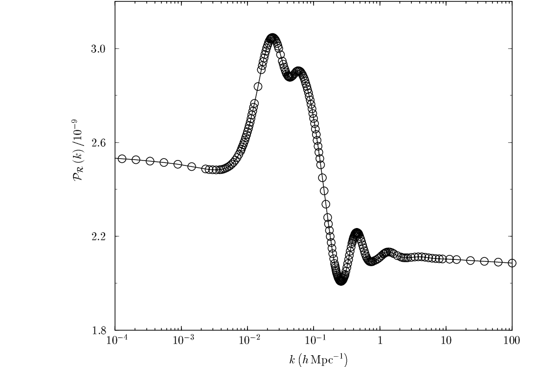
evaluated when the mode has crossed well outside the horizon. Rather than calculating $\mathcal{P}_{\mathcal{R}}$ in this way for every wavenumber, we use cubic spline interpolation between $\mathcal{O}\left(100\right)$ wavenumbers $k_{i}$ to save time. These sample the spectrum more densely where its curvature is higher, in order to minimise the interpolation error. The $k_{i}$ values are found each time using the adaptive sampling algorithm described in Appendix A.

Taking the interpolated primordial perturbation spectrum as input, we use a modified version of the cosmological Boltzmann code CAMB Lewis:1999bs to evaluate the CMB TT, TE and EE spectra, as well as the matter power spectrum.⁴⁴ 4 http://camb.info

We find the two-point correlation function using the following procedure: for $10^{-5}\leq k\leq 2\,h\,\mathrm{Mpc^{-1}}$ the linear matter power spectrum $P_{\mathrm{m}}(k)$ is obtained using CAMB, while outside this range baryon oscillations are negligible, and so to calculate the matter power spectrum $P_{\mathrm{m}}(k)$ for $10^{-6}\leq k\leq 10^{-5}\,h\,\mathrm{Mpc^{-1}}$ and $2\leq k\leq 10^{2}\,h\,\mathrm{Mpc^{-1}}$ we use the no-baryon transfer function fitting formula of ref.Eisenstein:1997ik normalised to the CAMB transfer function. This significantly increases the speed of the computation. The ‘Halofit’ procedure Smith:2002dz is then used to apply the corrections from non-linear evolution to produce the non-linear matter power spectrum $P_{\mathrm{m}}^{\mathrm{NL}}\left(k\right)$ . The LRG power spectrum is given by $P_{\mathrm{LRG}}(k)=b_{\mathrm{LRG}}^{2}P_{\mathrm{m}}^{\mathrm{NL}}(k)$ . The real space correlation function $\xi_{\rm c}(x)$ is then calculated by taking the Fourier transform. The integral is performed over a finite range of $k$ using the FFTLog code Hamilton:1999uv which takes the fast Fourier transform of a series of logarithmically spaced points. The wavenumber range must be broad enough to prevent ringing and aliasing effects from the FFT over the interval of $x$ for which we require $\xi_{\rm c}$ . We find the range $10^{-6}\leq k\leq 10^{2}\,h\,\mathrm{Mpc^{-1}}$ to be sufficient. Finally, the angle averaged redshift correlation function is found from the real space correlation function using

\xi(x)=\left(1+\frac{2}{3}f+\frac{1}{5}f^{2}\right)\xi_{\rm c}(x),\qquad f\equiv\frac{\Omega_{\mathrm{m}}^{3/5}}{b_{\rm LRG}},

(24)

which corrects for redshift space distortion effects Kaiser:1987qv; Hamilton:1991es.

V Results

We calculate the mean values of the marginalised cosmological parameters together with their $68$ % confidence limits, for the four combinations of data sets: WMAP, WMAP + SDSS, WMAP + LRG, WMAP + SDSS + LRG. In Table 4 we show this for the $\Lambda$ CDM model with a Harrison-Zeldovich spectrum. Adding an overall ‘tilt’ to the spectrum creates a noticeable improvement (by $\Delta\chi^{2}\sim 7-9$ ) as is seen from Table 5 which gives results for the $\Lambda$ CDM model with a power-law scalar spectral index of $n_{\mathrm{s}}\simeq 0.95$ (pivot point $k=0.05\,\mathrm{Mpc}^{-1}$ ). The $\chi^{2}$ goodness-of-fit statistic is calculated using the WMAP likelihood code, supplemented by our estimate for the LRG fits obtained using the covariance matrix used in ref.Eisenstein:2005su.

In order to quantify the desirable compromise between improving the fit and adding new parameters, it has become customary to use the “Akaike information criterion” defined as $\mathrm{AIC}\equiv-2\ln{\cal L}_{\mathrm{max}}+2N$ Akaike:1974, where ${\cal L}_{\mathrm{max}}$ is the maximum likelihood and $N$ the number of parameters. Although not a substitute for a full Bayesian evidence calculation (which is beyond the scope of this work), this is a commonly used guide for judging whether additional parameters are justified — the model with the minimum AIC value is in some sense preferred Liddle:2004nh. According to this criterion, the power-law $\Lambda$ CDM model is preferred over the scale-invariant $\Lambda$ CDM model, hence we consider the former to be the benchmark against which our models should be judged. However we wish to emphasise that we have physical motivation for the non-standard primordial spectra we consider. We are not performing a pure parameter fitting exercise for which criteria like the AIC might be more relevant.

	WMAP	+SDSS	+LRG	+SDSS+LRG
$\Omega_{\mathrm{b}}h^{2}$	$0.02381_{-0.00043}^{+0.00042}$	$0.02393_{-0.00039}^{+0.00039}$	$0.02395_{-0.00038}^{+0.00037}$	$0.02394_{-0.00038}^{+0.00038}$
$\Omega_{\mathrm{c}}h^{2}$	$0.1031_{-0.0079}^{+0.0077}$	$0.1131_{-0.0052}^{+0.0054}$	$0.1163_{-0.0045}^{+0.0046}$	$0.1173_{-0.0041}^{+0.0041}$
$\theta$	$1.0451_{-0.0027}^{+0.0029}$	$1.0463_{-0.0028}^{+0.0027}$	$1.0465_{-0.0028}^{+0.0029}$	$1.0465_{-0.0026}^{+0.0027}$
$\tau$	$0.139_{-0.013}^{+0.013}$	$0.129_{-0.012}^{+0.014}$	$0.123_{-0.011}^{+0.012}$	$0.120_{-0.012}^{+0.012}$
$\ln\left(10^{10}\mathcal{P_{R}}\right)$	$3.137_{-0.052}^{+0.055}$	$3.160_{-0.049}^{+0.050}$	$3.161_{-0.049}^{+0.051}$	$3.158_{-0.047}^{+0.053}$
$b_{\mathrm{LRG}}$			$2.123_{-0.091}^{+0.089}$	$2.129_{-0.093}^{+0.093}$
$\Omega_{\Lambda}$	$0.785_{-0.029}^{+0.029}$	$0.746_{-0.022}^{+0.021}$	$0.732_{-0.018}^{+0.018}$	$0.728_{-0.017}^{+0.017}$
Age/Gyr	$13.403_{-0.090}^{+0.091}$	$13.423_{-0.091}^{+0.091}$	$13.432_{-0.094}^{+0.092}$	$13.438_{-0.084}^{+0.088}$
$\Omega_{\mathrm{b}}$	$0.215_{-0.029}^{+0.029}$	$0.254_{-0.021}^{+0.022}$	$0.268_{-0.018}^{+0.018}$	$0.272_{-0.017}^{+0.017}$
$\sigma_{8}$	$0.801_{-0.050}^{+0.049}$	$0.856_{-0.032}^{+0.033}$	$0.870_{-0.031}^{+0.030}$	$0.873_{-0.029}^{+0.029}$
$z_{\mathrm{reion}}$	$14.5_{-2.0}^{+2.0}$	$14.1_{-2.1}^{+2.0}$	$13.7_{-1.9}^{+2.1}$	$13.5_{-2.0}^{+2.2}$
$h$	$0.772_{-0.029}^{+0.030}$	$0.736_{-0.020}^{+0.018}$	$0.724_{-0.015}^{+0.014}$	$0.721_{-0.014}^{+0.014}$
$\chi^{2}$	$11260$	$11279$	$11284$	$11301$
$\Delta_{\mathrm{AIC}}$	$5$	$6$	$7$	$7$

Table 4:

1\sigma

constraints on the marginalised cosmological parameters for a scale-invariant

\Lambda

CDM model. The 6 parameters in the upper part of the Table are varied by CosmoMC, while those in the lower part are derived quantities. The

\chi^{2}

of the fit is given, as is the Akaike information criterion relative to the power-law

\Lambda

CDM model in Table 5.

	WMAP	+SDSS	+LRG	+SDSS+LRG
$\Omega_{\mathrm{b}}h^{2}$	$0.02219_{-0.00070}^{+0.00070}$	$0.02236_{-0.00069}^{+0.00066}$	$0.02229_{-0.00068}^{+0.00069}$	$0.02240_{-0.00067}^{+0.00064}$
$\Omega_{\mathrm{c}}h^{2}$	$0.1052_{-0.0084}^{+0.0084}$	$0.1147_{-0.0054}^{+0.0056}$	$0.1147_{-0.0044}^{+0.0043}$	$0.1168_{-0.0038}^{+0.0038}$
$\theta$	$1.0391_{-0.0037}^{+0.0038}$	$1.0406_{-0.0036}^{+0.0036}$	$1.0403_{-0.0035}^{+0.0035}$	$1.0410_{-0.0033}^{+0.0033}$
$\tau$	$0.089_{-0.014}^{+0.014}$	$0.083_{-0.013}^{+0.014}$	$0.080_{-0.013}^{+0.013}$	$0.080_{-0.013}^{+0.013}$
$n_{\mathrm{s}}$	$0.9537_{-0.0081}^{+0.0072}$	$0.9542_{-0.0070}^{+0.0075}$	$0.9527_{-0.0075}^{+0.0072}$	$0.9547_{-0.0072}^{+0.0068}$
$\ln\left(10^{10}\mathcal{P_{R}}\right)$	$3.017_{-0.065}^{+0.065}$	$3.046_{-0.062}^{+0.061}$	$3.039_{-0.062}^{+0.062}$	$3.048_{-0.060}^{+0.060}$
$b_{\mathrm{LRG}}$			$2.26_{-0.10}^{+0.10}$	$2.25_{-0.10}^{+0.10}$
$\Omega_{\Lambda}$	$0.758_{-0.037}^{+0.037}$	$0.716_{-0.027}^{+0.028}$	$0.716_{-0.020}^{+0.020}$	$0.708_{-0.018}^{+0.019}$
Age/Gyr	$13.75_{-0.17}^{+0.16}$	$13.75_{-0.15}^{+0.15}$	$13.77_{-0.15}^{+0.15}$	$13.75_{-0.14}^{+0.14}$
$\Omega_{\mathrm{m}}$	$0.242_{-0.037}^{+0.037}$	$0.284_{-0.028}^{+0.027}$	$0.284_{-0.020}^{+0.020}$	$0.292_{-0.019}^{+0.018}$
$\sigma_{8}$	$0.754_{-0.050}^{+0.049}$	$0.804_{-0.034}^{+0.035}$	$0.801_{-0.035}^{+0.036}$	$0.813_{-0.032}^{+0.031}$
$z_{\mathrm{reion}}$	$11.1_{-2.4}^{+2.5}$	$10.8_{-2.4}^{+2.5}$	$10.5_{-2.5}^{+2.5}$	$10.5_{-2.6}^{+2.6}$
$h$	$0.730_{-0.034}^{+0.034}$	$0.697_{-0.023}^{+0.024}$	$0.695_{-0.017}^{+0.017}$	$0.691_{-0.016}^{+0.016}$
$\chi^{2}$	$11253$	$11271$	$11275$	$11292$
$\Delta_{\mathrm{AIC}}$	$0$	$0$	$0$	$0$

Table 5:

1\sigma

constraints on the marginalised cosmological parameters for the power-law

\Lambda

CDM model. The 6 parameters in the upper part of the Table are varied by CosmoMC, while those in the lower part are derived quantities. The

\chi^{2}

of the fit is given as is the relative Akaike information criterion (normalised to be zero for this model).

V.1 $\Lambda$ CDM ‘step’ model

In Tables 6 to 9 we show that adding a step to the spectrum improves the fit by $\Delta\chi^{2}\sim 1-2$ relative to the scale-invariant model, but not as much as addition of a tilt. Since the model has 2 additional parameters — the position of the step $k_{1}$ and $n$ (which determines $\Delta m^{2}$ ) — $\Delta_{\mathrm{AIC}}$ is positive relative to the power-law $\Lambda$ CDM model.

We have not shown the results for the $\Lambda$ CDM step model allowing an overall tilt in the spectrum; although the fits do improve again (by $\Delta\chi^{2}\sim 1-2$ ) relative to the power-law $\Lambda$ CDM model, they are not favoured by the AIC because of the 2 additional parameters $k_{1}$ and $n$ . The values of the background cosmological parameters do not change significantly with $n$ either, and remain similar to those of the power-law $\Lambda$ CDM model. However, the values of both $\mathcal{P_{R}}^{\left(1\right)}$ and $k_{1}$ fall with increasing $n$ , as seen in the 1-D likelihood distributions for the parameters shown in Fig.1.

$n$	12	13	14	15	16	17
$\Omega_{\mathrm{b}}h^{2}$	$0.02366_{-0.00043}^{+0.00042}$	$0.02366_{-0.00046}^{+0.00045}$	$0.02363_{-0.00046}^{+0.00046}$	$0.02362_{+0.00045}^{+0.00045}$	$0.02370_{-0.00044}^{+0.00044}$	$0.02371_{-0.00045}^{+0.00046}$
$\Omega_{\mathrm{c}}h^{2}$	$0.1030_{-0.0079}^{+0.0083}$	$0.1022_{-0.0082}^{+0.0084}$	$0.1002_{-0.0086}^{+0.0083}$	$0.1002_{-0.0083}^{+0.0080}$	$0.1006_{-0.0084}^{+0.0085}$	$0.1017_{-0.0087}^{+0.0086}$
$\theta$	$1.0446_{-0.0029}^{+0.0030}$	$1.0445_{-0.0031}^{+0.0030}$	$1.0444_{-0.0030}^{+0.0029}$	$1.0445_{-0.0029}^{+0.0030}$	$1.0450_{-0.0031}^{+0.0031}$	$1.0451_{-0.0030}^{+0.0029}$
$\tau$	$0.151_{-0.014}^{+0.014}$	$0.157_{-0.016}^{+0.016}$	$0.159_{-0.017}^{+0.015}$	$0.148_{-0.015}^{+0.013}$	$0.142_{-0.012}^{+0.013}$	$0.129_{-0.012}^{+0.014}$
$10^{4}k_{1}/\mathrm{Mpc}^{-1}$	$20.8_{-7.1}^{+4.8}$	$14.9_{-6.2}^{+5.6}$	$9.5_{-3.4}^{+0.7}$	$6.1_{-2.3}^{+1.8}$	$4.9_{-1.9}^{+2.5}$	$3.2_{-1.6}^{+0.4}$
$\ln\left(10^{10}\mathcal{P_{R}}^{(0)}\right)$	$3.090_{-0.050}^{+0.053}$	$2.941_{-0.059}^{+0.057}$	$2.678_{-0.054}^{+0.055}$	$2.260_{-0.047}^{+0.046}$	$1.648_{-0.038}^{+0.037}$	$0.738_{-0.033}^{+0.035}$
$\Omega_{\Lambda}$	$0.784_{-0.031}^{+0.030}$	$0.787_{-0.031}^{+0.031}$	$0.795_{-0.030}^{+0.031}$	$0.795_{-0.030}^{+0.031}$	$0.795_{-0.031}^{+0.031}$	$0.791_{-0.032}^{+0.033}$
Age/Gyr	$13.432_{-0.094}^{+0.092}$	$13.418_{-0.097}^{+0.097}$	$13.418_{-0.097}^{+0.097}$	$13.415_{-0.098}^{+0.096}$	$13.395_{-0.096}^{+0.094}$	$13.400_{-0.091}^{+0.090}$
$\Omega_{\mathrm{m}}$	$0.216_{-0.030}^{+0.031}$	$0.213_{-0.031}^{+0.031}$	$0.205_{-0.031}^{+0.030}$	$0.205_{-0.031}^{+0.030}$	$0.205_{-0.031}^{+0.031}$	$0.209_{-0.033}^{+0.032}$
$\sigma_{8}$	$0.808_{-0.049}^{+0.050}$	$0.808_{-0.055}^{+0.054}$	$0.796_{-0.047}^{+0.050}$	$0.788_{-0.049}^{+0.049}$	$0.787_{-0.050}^{+0.050}$	$0.784_{-0.053}^{+0.052}$
$z_{\mathrm{reion}}$	$15.4_{-2.0}^{+2.0}$	$15.8_{-2.2}^{+2.3}$	$15.8_{-2.3}^{+2.4}$	$15.1_{-2.1}^{+2.1}$	$14.7_{-1.9}^{+1.9}$	$13.8_{-2.1}^{+2.1}$
$h$	$0.770_{-0.031}^{+0.030}$	$0.773_{-0.031}^{+0.032}$	$0.781_{-0.032}^{+0.032}$	$0.782_{-0.032}^{+0.032}$	$0.782_{-0.033}^{+0.033}$	$0.778_{-0.033}^{+0.034}$
$\Delta m^{2}$	$0.07193_{-0.00072}^{+0.00077}$	$0.1419_{-0.0015}^{+0.0015}$	$0.2455_{-0.0022}^{+0.0022}$	$0.3815_{-0.0028}^{+0.0027}$	$0.5417_{-0.0029}^{+0.0028}$	$0.7058_{-0.0031}^{+0.0033}$
$\chi^{2}$	$11259$	$11258$	$11258$	$11258$	$11259$	$11259$
$\Delta_{\mathrm{AIC}}$	$8$	$7$	$7$	$7$	$8$	$8$

Table 6: 1

\sigma

constraints on the marginalised cosmological parameters for the

\Lambda

CDM step model using WMAP data alone. The 6 parameters in the upper part of the Table are varied by CosmoMC, while those in the lower part are derived quantities. The

\chi^{2}

of the fit is given, as is the Akaike information criterion relative to the power-law

\Lambda

CDM model in Table 5 (taking into account that

n

is also a parameter).

$n$	12	13	14	15	16	17
$\Omega_{\mathrm{b}}h^{2}$	$0.02382_{-0.00040}^{+0.00042}$	$0.02381_{-0.00039}^{+0.00042}$	$0.02381_{-0.00043}^{+0.00040}$	$0.02383_{-0.00038}^{+0.00039}$	$0.02385_{-0.00041}^{+0.00041}$	$0.02393_{-0.00040}^{+0.00039}$
$\Omega_{\mathrm{c}}h^{2}$	$0.1132_{-0.0053}^{+0.0055}$	$0.1126_{-0.0056}^{+0.0058}$	$0.1130_{-0.0056}^{+0.0055}$	$0.1127_{-0.0054}^{+0.0057}$	$0.1130_{-0.0055}^{+0.0055}$	$0.1133_{+0.0055}^{+0.0054}$
$\theta$	$1.0460_{-0.0029}^{+0.0028}$	$1.0458_{-0.0029}^{+0.0030}$	$1.0459_{-0.0028}^{+0.0029}$	$1.0459_{-0.0027}^{+0.0028}$	$1.0461_{-0.0029}^{+0.0029}$	$1.0469_{-0.0029}^{+0.0029}$
$\tau$	$0.138_{-0.013}^{+0.014}$	$0.144_{-0.015}^{+0.016}$	$0.138_{-0.016}^{+0.012}$	$0.133_{-0.013}^{+0.013}$	$0.128_{-0.012}^{+0.014}$	$0.118_{-0.012}^{+0.014}$
$10^{4}k_{1}/\mathrm{Mpc}^{-1}$	$21.1_{-7.9}^{+4.6}$	$14.1_{-6.6}^{+6.2}$	$7.1_{-3.1}^{+1.0}$	$4.9_{-1.9}^{+2.0}$	$3.5_{-1.2}^{+0.4}$	$2.5_{-1.1}^{+0.9}$
$\ln\left(10^{10}\mathcal{P_{R}}^{(0)}\right)$	$3.107_{-0.049}^{+0.051}$	$2.959_{-0.051}^{+0.054}$	$2.691_{-0.048}^{+0.051}$	$2.280_{-0.041}^{+0.043}$	$1.667_{-0.039}^{+0.039}$	$0.755_{-0.029}^{+0.032}$
$\Omega_{\Lambda}$	$0.746_{-0.022}^{+0.023}$	$0.747_{-0.023}^{+0.023}$	$0.745_{-0.023}^{+0.023}$	$0.747_{-0.022}^{+0.023}$	$0.746_{-0.023}^{+0.023}$	$0.746_{-0.022}^{+0.022}$
Age/Gyr	$13.443_{-0.092}^{+0.094}$	$13.446_{-0.096}^{+0.095}$	$13.443_{-0.095}^{+0.094}$	$13.441_{-0.087}^{+0.092}$	$13.435_{-0.094}^{+0.094}$	$13.407_{-0.095}^{+0.092}$
$\Omega_{\mathrm{m}}$	$0.255_{-0.023}^{+0.024}$	$0.253_{-0.023}^{+0.024}$	$0.255_{-0.023}^{+0.023}$	$0.253_{-0.023}^{+0.022}$	$0.254_{-0.023}^{+0.023}$	$0.254_{-0.022}^{+0.022}$
$\sigma_{8}$	$0.863_{-0.033}^{+0.034}$	$0.864_{-0.035}^{+0.035}$	$0.862_{-0.034}^{+0.033}$	$0.856_{-0.033}^{+0.034}$	$0.853_{-0.033}^{+0.034}$	$0.849_{-0.034}^{+0.034}$
$z_{\mathrm{reion}}$	$14.8_{-2.0}^{+2.1}$	$15.2_{-2.2}^{+2.3}$	$14.8_{-2.2}^{+2.2}$	$14.4_{-2.0}^{+2.1}$	$14.0_{-2.1}^{+2.1}$	$13.3_{-2.0}^{+2.1}$
$h$	$0.734_{-0.019}^{+0.019}$	$0.735_{-0.020}^{+0.020}$	$0.734_{-0.019}^{+0.020}$	$0.736_{-0.019}^{+0.020}$	$0.735_{-0.020}^{+0.019}$	$0.737_{-0.018}^{+0.019}$
$\Delta m^{2}$	$0.07219_{-0.00070}^{+0.00073}$	$0.1424_{-0.0013}^{+0.0014}$	$0.2460_{-0.0020}^{+0.0021}$	$0.3826_{-0.0024}^{+0.0025}$	$0.5431_{-0.0030}^{+0.0030}$	$0.7074_{-0.0028}^{+0.0030}$
$\chi^{2}$	$11278$	$11278$	$11277$	$11278$	$11278$	$11278$
$\Delta_{\mathrm{AIC}}$	$9$	$9$	$8$	$9$	$9$	$9$

Table 7: 1

\sigma

constraints on the marginalised cosmological parameters for the

\Lambda

CDM step model using WMAP + SDSS data. The 6 parameters in the upper part of the Table are varied by CosmoMC, while those in the lower part are derived quantities. The

\chi^{2}

of the fit is given, as is the Akaike information criterion relative to the power-law

\Lambda

CDM model in Table 5 (taking into account that

n

is also a parameter).

$n$	12	13	14	15	16	17
$\Omega_{\mathrm{b}}h^{2}$	$0.02383_{-0.00039}^{+0.00039}$	$0.02384_{-0.00040}^{+0.00039}$	$0.02386_{-0.00041}^{+0.00040}$	$0.02388_{-0.00040}^{+0.00041}$	$0.02389_{-0.00040}^{+0.00041}$	$0.02393_{-0.00040}^{+0.00039}$
$\Omega_{\mathrm{c}}h^{2}$	$0.1160_{-0.0044}^{+0.0044}$	$0.1159_{-0.0046}^{+0.0045}$	$0.1159_{-0.0045}^{+0.0046}$	$0.1159_{-0.0047}^{+0.0045}$	$0.1159_{-0.0044}^{+0.0047}$	$0.1163_{-0.0044}^{+0.0044}$
$\theta$	$1.0460_{-0.0029}^{+0.0029}$	$1.0460_{-0.0028}^{+0.0028}$	$1.0461_{-0.0027}^{+0.0027}$	$1.0464_{-0.0028}^{+0.0030}$	$1.0465_{-0.0028}^{+0.0029}$	$1.0468_{-0.0028}^{+0.0028}$
$\tau$	$0.133_{-0.013}^{+0.013}$	$0.137_{-0.014}^{+0.013}$	$0.128_{-0.013}^{+0.012}$	$0.125_{-0.012}^{+0.013}$	$0.120_{-0.011}^{+0.013}$	$0.113_{-0.012}^{+0.014}$
$10^{4}k_{1}/\mathrm{Mpc}^{-1}$	$20.2_{-8.3}^{+4.8}$	$13.1_{-6.5}^{+6.4}$	$6.3_{-2.2}^{+1.5}$	$4.8_{-1.8}^{+1.8}$	$3.5_{-1.0}^{+0.4}$	$2.5_{-1.1}^{+1.0}$
$\ln\left(10^{10}\mathcal{P_{R}}^{(0)}\right)$	$3.108_{-0.048}^{+0.050}$	$2.957_{-0.051}^{+0.053}$	$2.683_{-0.047}^{+0.047}$	$2.278_{-0.045}^{+0.045}$	$1.663_{-0.038}^{+0.038}$	$0.756_{-0.032}^{+0.032}$
$b_{\mathrm{LRG}}$	$2.104_{-0.092}^{+0.094}$	$2.100_{-0.092}^{+0.094}$	$2.117_{-0.089}^{+0.090}$	$2.119_{-0.091}^{+0.091}$	$2.135_{-0.092}^{+0.092}$	$2.143_{-0.091}^{+0.093}$
$\Omega_{\Lambda}$	$0.732_{-0.018}^{+0.018}$	$0.732_{-0.018}^{+0.018}$	$0.733_{-0.020}^{+0.019}$	$0.734_{-0.019}^{+0.019}$	$0.734_{-0.019}^{+0.018}$	$0.733_{-0.019}^{+0.018}$
Age/Gyr	$13.456_{-0.095}^{+0.094}$	$13.454_{-0.090}^{+0.093}$	$13.450_{-0.093}^{+0.088}$	$13.440_{-0.098}^{+0.096}$	$13.436_{-0.094}^{+0.095}$	$13.425_{-0.093}^{+0.095}$
$\Omega_{\mathrm{m}}$	$0.268_{-0.018}^{+0.018}$	$0.267_{-0.018}^{+0.018}$	$0.267_{-0.019}^{+0.020}$	$0.266_{-0.019}^{+0.019}$	$0.266_{-0.018}^{+0.019}$	$0.267_{-0.019}^{+0.019}$
$\sigma_{8}$	$0.878_{-0.032}^{+0.032}$	$0.878_{-0.032}^{+0.032}$	$0.870_{-0.031}^{+0.031}$	$0.869_{-0.031}^{+0.031}$	$0.864_{-0.030}^{+0.031}$	$0.861_{-0.031}^{+0.031}$
$z_{\mathrm{reion}}$	$14.5_{-2.0}^{+2.1}$	$14.8_{-2.2}^{+2.3}$	$14.1_{-2.1}^{+2.1}$	$13.9_{-2.1}^{+2.2}$	$13.4_{-2.1}^{+2.1}$	$12.9_{-2.2}^{+2.2}$
$h$	$0.708_{-0.015}^{+0.015}$	$0.724_{-0.015}^{+0.015}$	$0.724_{-0.016}^{+0.016}$	$0.725_{-0.015}^{+0.015}$	$0.726_{-0.015}^{+0.015}$	$0.725_{-0.015}^{+0.015}$
$\Delta m^{2}$	$0.07152_{-0.00069}^{+0.00072}$	$0.1423_{-0.0013}^{+0.0014}$	$0.2457_{-0.0019}^{+0.0019}$	$0.3825_{-0.0027}^{+0.0027}$	$0.5428_{-0.0029}^{+0.0029}$	$0.7075_{-0.0031}^{+0.0030}$
$\chi^{2}$	$11282$	$11282$	$11282$	$11282$	$11282$	$11283$
$\Delta_{\mathrm{AIC}}$	$9$	$9$	$9$	$9$	$9$	$10$

Table 8: 1

\sigma

constraints on the marginalised cosmological parameters for the

\Lambda

CDM step model using WMAP + LRG data. The 7 parameters in the upper part of the Table are varied by CosmoMC, while those in the lower part are derived quantities. The

\chi^{2}

of the fit is given, as is the Akaike information criterion relative to the power-law

\Lambda

CDM model in Table 5 (taking into account that

n

is also a parameter).

$n$	12	13	14	15	16	17
$\Omega_{\mathrm{b}}h^{2}$	$0.02386_{-0.00040}^{+0.00040}$	$0.02384_{-0.00039}^{+0.00039}$	$0.02385_{-0.00041}^{+0.00040}$	$0.02387_{-0.00040}^{+0.00040}$	$0.02391_{-0.00042}^{+0.00041}$	$0.02395_{-0.00040}^{+0.00039}$
$\Omega_{\mathrm{c}}h^{2}$	$0.1170_{-0.0040}^{+0.0039}$	$0.1172_{-0.0041}^{+0.0041}$	$0.1172_{-0.0040}^{+0.0040}$	$0.1171_{-0.0040}^{+0.0040}$	$0.1176_{-0.0043}^{+0.0040}$	$0.1174_{-0.0039}^{+0.0037}$
$\theta$	$1.0460_{-0.0028}^{+0.0028}$	$1.0461_{-0.0028}^{+0.0028}$	$1.0463_{-0.0028}^{+0.0028}$	$1.0467_{-0.0027}^{-0.0027}$	$1.0466_{-0.0027}^{+0.0027}$	$1.0469_{-0.0025}^{+0.0027}$
$\tau$	$0.130_{-0.012}^{+0.013}$	$0.135_{-0.014}^{+0.015}$	$0.126_{-0.014}^{+0.013}$	$0.124_{-0.012}^{+0.013}$	$0.118_{-0.011}^{+0.013}$	$0.111_{-0.012}^{+0.014}$
$10^{4}k_{1}/\mathrm{Mpc}^{-1}$	$19.1_{-9.3}^{+4.6}$	$13.1_{-6.4}^{+6.2}$	$6.5_{-2.6}^{+1.4}$	$4.4_{-1.6}^{+1.5}$	$3.2_{-1.0}^{+0.6}$	$2.5_{-1.1}^{+1.0}$
$\ln\left(10^{10}\mathcal{P_{R}}^{(0)}\right)$	$3.106_{-0.047}^{+0.049}$	$2.960_{-0.051}^{+0.051}$	$2.685_{-0.047}^{+0.047}$	$2.279_{-0.040}^{+0.040}$	$1.667_{-0.037}^{+0.037}$	$0.757_{-0.032}^{+0.031}$
$b_{\mathrm{LRG}}$	$2.110_{-0.089}^{+0.090}$	$2.098_{-0.091}^{+0.091}$	$2.118_{-0.094}^{+0.094}$	$2.122_{-0.088}^{+0.089}$	$2.133_{-0.091}^{+0.088}$	$2.143_{-0.092}^{+0.092}$
$\Omega_{\Lambda}$	$0.727_{-0.016}^{+0.016}$	$0.727_{-0.017}^{+0.017}$	$0.727_{-0.017}^{+0.017}$	$0.728_{-0.016}^{+0.016}$	$0.726_{-0.017}^{+0.017}$	$0.728_{-0.015}^{+0.016}$
Age/Gyr	$13.456_{-0.093}^{+0.090}$	$13.457_{-0.092}^{+0.093}$	$13.451_{-0.092}^{+0.092}$	$13.446_{-0.090}^{+0.091}$	$13.439_{-0.096}^{+0.093}$	$13.426_{-0.090}^{+0.089}$
$\Omega_{\mathrm{m}}$	$0.273_{-0.016}^{+0.016}$	$0.273_{-0.017}^{+0.017}$	$0.273_{-0.017}^{+0.017}$	$0.272_{-0.016}^{+0.016}$	$0.274_{-0.017}^{+0.017}$	$0.272_{-0.016}^{+0.015}$
$\sigma_{8}$	$0.879_{-0.028}^{+0.029}$	$0.884_{-0.029}^{+0.029}$	$0.877_{-0.029}^{+0.029}$	$0.874_{-0.028}^{+0.028}$	$0.873_{-0.030}^{+0.028}$	$0.866_{-0.029}^{+0.028}$
$z_{\mathrm{reion}}$	$14.3_{-2.0}^{+2.1}$	$14.7_{-2.2}^{+2.2}$	$14.0_{-2.2}^{+2.2}$	$13.8_{-2.0}^{+2.0}$	$13.4_{-2.1}^{+2.1}$	$12.8_{-2.2}^{+2.2}$
$h$	$0.719_{-0.014}^{+0.013}$	$0.719_{-0.013}^{+0.014}$	$0.720_{-0.014}^{+0.014}$	$0.720_{-0.013}^{+0.014}$	$0.720_{-0.013}^{+0.013}$	$0.722_{-0.013}^{+0.013}$
$\Delta m^{2}$	$0.07219_{-0.00068}^{+0.00071}$	$0.1424_{-0.0013}^{+0.0013}$	$0.2458_{-0.0020}^{+0.0020}$	$0.3826_{-0.0024}^{+0.0023}$	$0.5431_{-0.0029}^{+0.0029}$	$0.7076_{-0.0030}^{+0.0030}$
$\chi^{2}$	$11299$	$11299$	$11299$	$11299$	$11299$	$11299$
$\Delta_{\mathrm{AIC}}$	$9$	$9$	$9$	$9$	$9$	$9$

Table 9: 1

\sigma

constraints on the marginalised cosmological parameters for the

\Lambda

CDM step model using WMAP + SDSS + LRG data. The 7 parameters in the upper part of the Table are varied by CosmoMC, while those in the lower part are derived quantities. The

\chi^{2}

of the fit is given, as is the Akaike information criterion relative to the power-law

\Lambda

CDM model in Table 5 (taking into account that

n

is also a parameter).

Refer to caption — Figure 1: 1-dimensional likelihood distributions of the marginalised cosmological parameters for the $\Lambda$ CDM step model using the WMAP + SDSS + LRG data.

To understand this, recall that the amplitude of the primordial perturbation spectrum is well constrained by the TT spectrum on medium scales, but is uncertain on large scales due to cosmic variance. Therefore the data can accommodate a large step in $\mathcal{P_{R}}$ provided that the top of the step is at the right height to match the TT spectrum. Consequently $\mathcal{P_{R}}^{(0)}$ must vary with the inflaton mass change in such a way as to leave the primordial perturbation spectrum invariant on smaller scales. This is seen in Fig.2 which shows the primordial spectra for the best-fit models.

The position of the step in $\mathcal{P_{R}}(k)$ for $n=14$ means that the associated TT and TE spectra are lower on large scales than those of the best-fit power-law model — see Figs.3 and 4. For $n=15$ to $n=17$ the lower plateau of the step is too far outside the Hubble radius to suppress the TT and TE spectra. However the primordial spectrum has a prominent first peak at $k\simeq 6\times 10^{-4}$ $h$ Mpc^-1. This introduces a maximum in the TT spectrum centred on $\ell=4$ which fits the excess power seen there by WMAP. There is a corresponding peak at low $\ell$ in the TE spectrum. The peak at $k\simeq 1.5\times 10^{-3}\,h\,\mathrm{Mpc^{-1}}$ in the primordial spectrum (for $n=14$ to $n=17$ ) increases the amplitude of the TT spectrum around $\ell=15$ . However the glitches in the TT spectrum at $\ell=22$ and $\ell=40$ are too sharp to match the oscillations produced by the mechanism considered here.

As seen in Fig.6, the SDSS galaxy power spectrum is well matched in all cases but the features in the spectrum due to the phase transition appear far outside the scales probed by redshift surveys (see Fig.7). Moreover a step in the matter power spectrum does not significantly alter the two-point correlation function in a $\Lambda$ CDM universe as shown in Fig.8. Just as for the concordance power-law $\Lambda$ CDM model however, the amplitude of the predicted BAO peak is too low by a factor of $\sim 2$ , although its predicted position does match the data Blanchard:2005ev.

We conclude therefore that the observations favour a ‘tilted’ primordial spectrum over a scale-invariant one, as has been emphasised already by the WMAP team Spergel:2006hy. However the spectrum is not required to be scale-free. Very different primordial spectra (as shown in Fig.2) provide just as good a fit to the data, although this is admittedly penalised by the Akaike information criterion taking into account the 2 additional parameters characterising the step in the spectrum. This motivates us to ask whether even the best-fit cosmological model might be altered if a more radical departure from a scale-free spectrum is considered. For example in multiple inflation Adams:1997de, two phase transitions can occur in rapid succession resulting in a ‘bump’ in the primordial spectrum. Such a feature has been advocated earlier on empirical grounds for fitting a $\Lambda$ CDM model Silk:2000sn.

V.2 CHDM ‘bump’ model

We consider now a primordial spectrum with a bump at $k\simeq 2\times 10^{-3}\,h\,\mathrm{Mpc^{-1}}$ generated by 2 successive phase transitions which cause an upward step followed by a slightly larger downward step in the amplitude of the primordial perturbation, as shown in Fig.9. This boosts the amplitude of the TT spectrum on the left of the first acoustic peak but suppresses the second and third peaks. This is all that is necessary to fit the WMAP data to an Einstein-de Sitter cosmology as seen in Fig.10. Since there is no late ISW effect, the amplitude is smaller on large scales than in an universe with dark energy. The fits to the TE and EE spectra are also good as shown in Fig.11 and 12.

By adding a hot dark matter component in the form of massive neutrinos, the amplitude of the matter power spectrum on small scales is suppressed relative to a pure CDM model and a good fit obtained to SDSS data (see Fig.13). As noted earlier Blanchard:2003du, this suppresses $\sigma_{8}$ so as to provide better agreement with the value deduced from clusters and weak lensing. A further suppression occurs due to the downward step in the primordial spectrum.

The constraints on the marginalised cosmological parameters are given in Table 10 with the order of the non-renormalisable terms set to $n_{1}=12$ and $n_{2}=13$ (which we nevertheless count as 2 additional parameters). We also allow $n_{1}$ and $n_{2}$ to vary continuously (but find no further improvement), with the results shown in Table 11 and as 1-D likelihood distributions in Fig.14. The fit of this model to the WMAP data and the SDSS matter power spectrum is just as good as that of the power-law $\Lambda$ CDM model, as indicated by the $\chi^{2}$ values and the vanishing $\Delta_{\mathrm{AIC}}$ . However, as has been noted already Blanchard:2005ev, the CHDM model does not fit the LRG two-point correlation function well. This is because the BAO peak corresponds to the comoving sound horizon at baryon decoupling; the latter is a function of $\Omega_{\mathrm{m}}$ and is too low in an Einstein-de Sitter universe as seen in Fig.15.

	WMAP	+SDSS	+LRG	+SDSS+LRG
$\Omega_{\mathrm{b}}h^{2}$	$0.01748_{-0.00071}^{+0.00073}$	$0.01762_{-0.00078}^{+0.00080}$	$0.01692_{-0.00047}^{+0.00047}$	$0.01688_{-0.00045}^{+0.00044}$
$\theta$	$1.0365_{-0.0051}^{+0.0051}$	$1.0378_{-0.0049}^{+0.0049}$	$1.0300_{-0.0040}^{+0.0040}$	$1.0300_{-0.0039}^{+0.0039}$
$\tau$	$0.078_{-0.011}^{+0.012}$	$0.079_{-0.012}^{+0.012}$	$0.071_{-0.011}^{+0.011}$	$0.071_{-0.011}^{+0.012}$
$f_{\nu}$	$0.096_{-0.023}^{+0.017}$	$0.103_{-0.011}^{+0.011}$	$0.1360_{-0.0092}^{+0.0092}$	$0.1353_{-0.0067}^{+0.0075}$
$10^{4}k_{1}/\mathrm{Mpc}^{-1}$	$86_{-13}^{+15}$	$82_{-9.8}^{+11}$	$77_{-10}^{+12}$	$77_{-9.5}^{+11}$
$10^{4}k_{2}/\mathrm{Mpc}^{-1}$	$527_{-78}^{+78}$	$539_{-82}^{+84}$	$380_{-24}^{+24}$	$379_{-22}^{+22}$
$\ln\left(10^{10}\mathcal{P_{R}}^{(0)}\right)$	$3.282_{-0.047}^{+0.047}$	$3.276_{-0.046}^{+0.045}$	$3.270_{-0.046}^{+0.046}$	$3.270_{-0.047}^{+0.046}$
$b_{\mathrm{LRG}}$			$2.99_{-0.16}^{+0.16}$	$2.99_{-0.16}^{+0.16}$
$\Omega_{\mathrm{c}}h^{2}$	$0.155_{-0.011}^{+0.012}$	$0.1539_{-0.0083}^{+0.0084}$	$0.1387_{-0.0044}^{+0.0041}$	$0.1387_{-0.0036}^{+0.0037}$
$\Omega_{\mathrm{d}}h^{2}$	$0.1712_{-0.0062}^{+0.0063}$	$0.1715_{-0.0059}^{+0.0061}$	$0.1605_{-0.0031}^{+0.0030}$	$0.1604_{-0.0030}^{+0.0030}$
$\mathrm{Age/GYr}$	$15.01_{-0.27}^{+0.27}$	$14.99_{-0.27}^{+0.26}$	$15.48_{-0.14}^{+0.14}$	$15.48_{-0.14}^{+0.14}$
$\sigma_{8}$	$0.668_{-0.089}^{+0.093}$	$0.648_{-0.054}^{+0.053}$	$0.565_{-0.033}^{+0.032}$	$0.565_{-0.028}^{+0.029}$
$z_{\mathrm{reion}}$	$13.6_{-3.1}^{+3.1}$	$13.6_{-3.1}^{+3.0}$	$12.7_{-3.1}^{+3.1}$	$12.7_{-3.2}^{+3.1}$
$h$	$0.4344_{-0.0077}^{+0.0078}$	$0.4348_{-0.0076}^{+0.0079}$	$0.4212_{-0.0038}^{+0.0037}$	$0.4211_{-0.0038}^{+0.0038}$
$\Delta m_{1}^{2}$	$0.07476_{-0.00071}^{+0.00070}$	$0.07468_{-0.00069}^{+0.00068}$	$0.07459_{-0.00069}^{+0.00068}$	$0.07459_{-0.00070}^{+0.00068}$
$\Delta m_{2}^{2}$	$0.1510_{-0.0013}^{+0.0013}$	$0.1508_{-0.0013}^{+0.0012}$	$0.1507_{-0.0013}^{+0.0012}$	$0.1507_{-0.0013}^{+0.0012}$
$\widetilde{t}_{2}-\widetilde{t}_{1}$	$1.82_{-0.18}^{+0.16}$	$1.89_{-0.19}^{+0.15}$	$1.62_{-0.17}^{+0.12}$	$1.62_{-0.17}^{+0.11}$
$\chi^{2}$	$11247$	$11265$	$11297$	$11315$
$\Delta_{\mathrm{AIC}}$	$0$	$0$	$28$	$29$

Table 10:

1\sigma

constraints on the marginalised cosmological parameters for the CHDM bump model, with the changes in the inflaton mass set by choosing

n_{1}=12

n_{2}=13

(which are still counted as 2 additional free parameters). The 8 parameters in the upper part of the Table are varied by CosmoMC, while those in the lower part are derived quantities. The

\chi^{2}

of the fit is given, as is the Akaike information criterion relative to the power-law

\Lambda

CDM model in Table 5.

	WMAP	+SDSS	+LRG	+SDSS+LRG
$\Omega_{\mathrm{b}}h^{2}$	$0.0173_{-0.0013}^{+0.0013}$	$0.0175_{-0.0012}^{+0.0012}$	$0.01724_{-0.00097}^{+0.00098}$	$0.01739_{-0.00099}^{+0.00098}$
$\theta$	$1.0364_{-0.0062}^{+0.0061}$	$1.0374_{-0.0056}^{+0.0056}$	$1.0314_{-0.0052}^{+0.0053}$	$1.0319_{-0.0052}^{+0.0052}$
$\tau$	$0.075_{-0.012}^{+0.012}$	$0.075_{-0.012}^{+0.012}$	$0.071_{-0.012}^{+0.012}$	$0.073_{-0.012}^{+0.012}$
$f_{\nu}$	$0.088_{-0.025}^{+0.016}$	$0.094_{-0.014}^{+0.015}$	$0.1349_{-0.0085}^{+0.0088}$	$0.1354_{-0.0070}^{+0.0073}$
$10^{4}k_{1}/\mathrm{Mpc}^{-1}$	$88_{-15}^{+17}$	$85_{-13}^{+14}$	$83_{-16}^{+11}$	$80_{-13}^{+12}$
$10^{4}k_{2}/\mathrm{Mpc}^{-1}$	$586_{-90}^{+36}$	$585_{-82}^{+36}$	$385_{-27}^{+28}$	$386_{-27}^{+27}$
$\ln\left(10^{10}\mathcal{P}_{\mathcal{R}}^{\left(0\right)}\right)$	$3.285_{-0.057}^{+0.059}$	$3.287_{-0.057}^{+0.058}$	$3.289_{-0.060}^{+0.061}$	$3.290_{-0.059}^{+0.061}$
$\ln\left(10^{10}\mathcal{P}_{\mathcal{R}}^{\left(1\right)}\right)$	$3.435_{-0.050}^{+0.050}$	$3.429_{-0.049}^{+0.048}$	$3.418_{-0.048}^{+0.047}$	$3.421_{-0.049}^{+0.049}$
$\ln\left(10^{10}\mathcal{P}_{\mathcal{R}}^{\left(2\right)}\right)$	$3.088_{-0.067}^{+0.073}$	$3.091_{-0.067}^{+0.071}$	$3.132_{-0.056}^{+0.056}$	$3.140_{-0.058}^{+0.057}$
$b_{\mathrm{LRG}}$			$2.97_{-0.16}^{+0.16}$	$2.96_{-0.16}^{+0.16}$
$\Omega_{\mathrm{c}}h^{2}$	$0.157_{-0.014}^{+0.014}$	$0.156_{-0.011}^{+0.011}$	$0.1404_{-0.0055}^{+0.0054}$	$0.1407_{-0.0050}^{+0.0049}$
$\Omega_{\mathrm{d}}h^{2}$	$0.1723_{-0.0090}^{+0.0090}$	$0.1724_{-0.0077}^{+0.0079}$	$0.1622_{-0.0050}^{+0.0051}$	$0.1628_{-0.0050}^{+0.0050}$
$\mathrm{Age/GYr}$	$14.98_{-0.40}^{+0.40}$	$14.97_{-0.35}^{+0.35}$	$15.39_{-0.25}^{+0.25}$	$15.36_{-0.25}^{+0.25}$
$\sigma_{8}$	$0.678_{-0.099}^{+0.097}$	$0.662_{-0.064}^{+0.063}$	$0.572_{-0.036}^{+0.035}$	$0.574_{-0.031}^{+0.031}$
$z_{\mathrm{reion}}$	$13.2_{-3.3}^{+3.2}$	$13.2_{-3.2}^{+3.2}$	$12.5_{-3.1}^{+3.1}$	$12.8_{-3.2}^{+3.1}$
$h$	$0.435_{-0.012}^{+0.012}$	$0.436_{-0.010}^{+0.010}$	$0.4236_{-0.0068}^{+0.0070}$	$0.4244_{-0.0068}^{+0.0068}$
$\Delta m_{1}$	$0.072_{-0.022}^{+0.021}$	$0.068_{-0.023}^{+0.023}$	$0.062_{-0.025}^{+0.024}$	$0.064_{-0.024}^{+0.023}$
$\Delta m_{2}$	$0.176_{-0.030}^{+0.025}$	$0.172_{-0.028}^{+0.023}$	$0.145_{-0.018}^{+0.018}$	$0.141_{-0.018}^{+0.018}$
$\widetilde{t}_{2}-\widetilde{t}_{1}$	$1.91_{-0.28}^{+0.23}$	$1.93_{-0.24}^{+0.21}$	$1.61_{-0.21}^{+0.15}$	$1.63_{-0.21}^{+0.13}$
$\chi^{2}$	$11247$	$11265$	$11296$	$11315$
$\Delta_{\mathrm{AIC}}$	$0$	$0$	$27$	$29$

Table 11:

1\sigma

constraints on the marginalised cosmological parameters for the CHDM bump model, with the changes in the inflaton mass allowed to vary freely. The 10 parameters in the upper part of the Table are varied by CosmoMC, while those in the lower part are derived quantities. The

\chi^{2}

of the fit is given, as is the Akaike information criterion relative to the power-law

\Lambda

CDM model in Table 5.

VI Parameter degeneracies

If two different parameters have similar effects on an observable then they will be negatively correlated in a $2$ -D likelihood plot since the effect of increasing the value of one of them can be undone by decreasing the value of the other. On the other hand, if two parameters have opposite effects then increasing the value of one can compensate for increasing the value of the other and the parameters will be positively correlated. Such correlations are known as parameter degeneracies and they limit the constraints which the data can place on the parameter values.

VI.1 $\Lambda$ CDM ‘step’ model degeneracies

The results indicate a strong parameter degeneracy amongst the models with one phase transition. Moving in parameter space along the direction of the degeneracy, $\Delta m^{2}$ increases, while $\mathcal{P_{R}}^{(0)}$ and $k_{1}$ both decrease. This arises because the amplitude of the TT spectrum on the scale of the acoustic peaks is governed by the combination $\mathcal{P_{R}}^{(1)}\mathrm{e}^{-2\tau}$ , where $\mathcal{P_{R}}^{(1)}$ is the amplitude of the primordial spectrum after the phase transition:

P_{\mathcal{R}}^{(1)}=\frac{P_{\mathcal{R}}^{(0)}}{\left(1-\Delta m^{2}\right)^{2}}.

(25)

The fit to WMAP data thus requires $\mathcal{P_{R}}^{(1)}\propto\mathrm{e}^{2\tau}$ . Consequently $\tau$ at fixed $\Delta m^{2}$ is positively correlated with $\mathcal{P_{R}}^{(0)}$ (reflecting the well-known degeneracy between the optical depth and the normalisation of the TT spectrum). However $\tau$ falls going from $n=15$ to $n=17$ because decreasing $\tau$ reduces $P_{\mathcal{R}}^{(0)}$ , while increasing $\Delta m^{2}$ raises $P_{\mathcal{R}}^{(1)}$ .

The value of $\mathcal{P_{R}}^{(1)}$ is constrained after marginalising over $\tau$ , which means that the relationship between $\Delta m^{2}$ and $\mathcal{P_{R}}^{(0)}$ is fitted well by

P_{\mathcal{R}}^{(0)}=P_{\mathcal{R}}^{\rm HZ}\left(1-\Delta m^{2}\right)^{2},

(26)

where $P_{\mathcal{R}}^{\rm HZ}$ is a constant (being the amplitude of a scale-invariant Harrison-Zeldovich primordial spectrum). This is illustrated in Fig.16 using results from Table 9.

The parameter $k_{1}$ is negatively correlated with $\Delta m^{2}$ because the higher cosmic variance at low $\ell$ allows the data to accommodate more prominent features in the primordial spectrum at smaller $k$ . The likelihood distribution of $k_{1}$ is strongly non-Gaussian, as shown in Fig.1. Each distribution has maxima wherever the oscillations in the corresponding TT spectrum due to the phase transition match the glitches in the WMAP measurements.

VI.2 CHDM ‘bump’ model degeneracies

The CHDM bump model has several parameter degeneracies which are illustrated in Fig.17. There is a positive correlation between the optical depth and the amplitude of the primordial spectrum on medium and small scales. The correlation between $\tau$ and $P_{\mathcal{R}}^{(1)}$ is weaker because reionisation does not damp the TT spectrum on large scales.

Increasing the baryon density increases the height of the first acoustic peak relative to the second one Hu:1995en, while increasing $\Delta m^{2}_{2}$ increases the size of the second step in the primordial spectrum and so boosts the height of the first peak relative to the other peaks. Thus $\omega_{\rm b}$ and $\Delta m_{2}^{2}$ are negatively correlated since both parameters have the same effect on the height of the first peak relative to the second Hu:1995en.

The bump in the primordial spectrum becomes broader when $k_{1}$ is increased, which increases the height of the second acoustic peak relative to the third. Reducing the density of CDM has a similar effect on the peak heights, hence $k_{1}$ and $\omega_{\rm c}$ are positively correlated. The baryon and CDM densities are also positively correlated because increasing $\omega_{\rm b}$ increases the height of the first acoustic peak, while increasing $\omega_{\rm c}$ has the opposite effect Hu:1995en.

The error bars of the WMAP data are smallest in the region of the first acoustic peak, so $P_{\mathcal{R}}^{(1)}$ is more tightly constrained than $P_{\mathcal{R}}^{(0)}$ or $P_{\mathcal{R}}^{(2)}$ , as is apparent from Table 11. Consequently the parameters $P_{\mathcal{R}}^{(0)}$ and $\Delta m_{1}^{2}$ satisfy

P_{\mathcal{R}}^{(0)}=P_{\mathcal{R}}^{\mathrm{HZ}}\left(1-\Delta m_{1}^{2}\right)^{2},

(27)

which is similar to eq.(26).

From the last equality of eq.(15) it is apparent that increasing $\Delta m_{2}^{2}$ reduces $\mathcal{P_{R}}^{(2)}$ , hence these parameters are anti-correlated, as seen in the final panel of Fig.17.

VII Conclusions

Anisotropies in the CMB and correlations in the large-scale distribution of galaxies reflect the primordial perturbations, presumably from inflation, but convoluted with the a priori unknown effects of their evolution in matter. Thus the values of the parameters of the assumed cosmological model are necessarily uncertain due to our limited knowledge of both the dark matter content of the universe, as well as of the nature of the primordial perturbations. Nevertheless, by combining various lines of evidence, it has been possible to make a strong case for the concordance $\Lambda$ CDM model, based on a FRW cosmology Peebles:2002gy. This model appears deceptively simple, but invokes vacuum energy at an unnatural scale, $\rho_{\Lambda}\sim(10^{-30}M_{\mathrm{P}})^{4}$ , as the dominant constituent of the universe. There is no satisfactory understanding of this from fundamental theoretical considerations Weinberg:1988cp; Nobbenhuis:2004wn. It is therefore worth reexamining whether the precision WMAP data, which has played a key role in the general acceptance of the $\Lambda$ CDM model, cannot be otherwise interpreted.

In this work we have focussed on the fact that our present understanding of the physics of inflation is rather primitive and there is no compelling reason why the generated primordial adiabatic scalar density perturbation should be close to the scale-invariant Harrison-Zeldovich form, as is usually assumed. This is indeed what is expected in the simplest toy model of an inflaton field evolving slowly down a suitably flat potential, but attempts to realise this in a physical theory such as supergravity or string/M-theory are plagued with difficulties. Such considerations strongly suggest moreover that even if just one scalar field comes to dominate the energy density and drives inflation, the non-trivial dynamics of other scalar fields in the inflating universe can affect its slow-roll evolution and thus create features in the primordial spectrum. Indeed there is some indication for such spectral features in the WMAP observations. Whether they are real rather than systematic effects will be tested further in the WMAP 5-yr analysis and by the forthcoming Planck mission unknown:2006uk. It has also been noted that significant non-Gaussianity would be generated when there are sharp features in the inflaton potential Chen:2006xj. This can be computed in our model and would constitute an independent test.

We have demonstrated that such spectral features can have a major impact on cosmological parameter estimation, in that the WMAP data can be fitted without requiring any dark energy, if there happens to be a mild bump in the primordial spectrum on spatial scales of order the Hubble radius at the last scattering surface. This has been modelled here using the supergravity-based multiple inflation model Adams:1997de with reasonable choices for the model parameters. Although other possibilities for generating spectral features have been investigated, our framework has the advantage of being based on effective field theory and thus calculable.

We have also departed from earlier work on parameter estimation in considering possible values of the Hubble constant well below the HKP value Freedman:2000cf which is usually input as a prior. Moreover the CHDM ‘bump’ model cannot fit the luminosity distance measurements of SN Ia, since the supernovae are fainter than predicted in a homogeneous Einstein-de Sitter cosmology. However, it has been noted that deep measurements using physical methods yield a lower value of $h$ than that measured locally Freedman:2000cf; Blanchard:2003du as would be the case if we are located in an underdense void which is expanding faster than the average Zehavi:1998gz. There are ongoing attempts to test whether we are indeed inside such a ‘Hubble bubble’ Jha:2006fm; Conley:2007ng. This is enormously important since such an inhomogeneous LTB cosmology can in principle address the failures of our FRW framework, with regard to the SN Ia Hubble diagram and the BAO peak Biswas:2006ub.

Moreover we have shown that the observed power spectrum of galaxy clustering can also be accounted for by modifying the nature of the dark matter, in particular allowing for a significant component due to massive neutrinos. Whether neutrinos do have the required mass of $\sim 0.5$ eV will be definitively tested in the forthcoming KATRIN experiment Drexlin:2004as. The position of the baryon peak seen in the galaxy correlation function may also be matched in the LTB framework, with a low global Hubble constant Biswas:2006ub.

Regardless of whether this model is the right description of the physical universe, we wish to emphasise that it provides a good fit to the WMAP data. Thus for progress to be made in pinning down the cosmological parameters and extending our understanding of inflation using precision CMB data, it is clearly necessary for a broader analysis framework to be adopted than has been the practice so far.

Acknowledgements.

We thank Graham Ross for discussions concerning inflation and Jo Dunkley and Alex Lewis for advice on MCMC codes. We are grateful to the WMAP team for making their data and analysis tools publicly available, and to the Referee for helpful suggestions. This work was supported by a STFC Senior Fellowship award (PPA/C506205/1) and by the EU Marie Curie Network “UniverseNet” (HPRN-CT-2006-035863).

Appendix A adaptive sampling algorithm

For plotting or interpolating a function $y=f(x)$ over an interval $(x_{\mathrm{min}},x_{\mathrm{max}})$ it is useful to have an algorithm that generates a set of points $\left\{x_{i},f\left(x_{i}\right)\right\}$ , where $x_{i+1}>x_{i}$ , such that the density of the samples $x_{i}$ in the abscissa increases with $\mathrm{d}^{2}f/\mathrm{d}x^{2}$ . One such algorithm is listed here. It works by ensuring that the value of the function at the mid-point of each interval $(x_{i},x_{i+2})$ is within some tolerance $\varepsilon$ of the value there linearly interpolated from the end-points of the interval.

1.

Form two lists $\{x_{1},x_{2},\ldots,x_{N}\}$ and $\{y_{1},y_{2},\ldots,y_{N}\}$ where the $x_{i}^{\prime}s$ are equally spaced,

$x_{i}=x_{\mathrm{min}}+\left(\frac{i-1}{N-1}\right)x_{\mathrm{max}},\quad i=1,2,\ldots,N,$ (28)

and $y_{i}=f\left(x_{i}\right)$ .
2.

Start with the first interval $(x_{1},x_{2}).$
3.

For the interval $(x_{i},x_{i+1})$ under consideration calculate $x_{m}\equiv\left(x_{i}+x_{i+1}\right)/2$ and $y_{m}\equiv f(x_{m})$ . Insert $x_{m}$ between $x_{i}$ and $x_{i+1}$ in the list of $x$ values and $y_{m}$ between $y_{i}$ and $y_{i+1}$ in the list of $y$ values.
4.

If $\left|y_{m}-\left(y_{i}+y_{i+1}\right)/2\right|>\varepsilon$ repeat step $3$ with the new interval $(x_{i},x_{m})$ .
5.

Otherwise repeat step $3$ with the next interval $\left(x_{i+1},x_{i+2}\right)$ , unless $x_{i+1}=x_{\rm max}$ , in which case finish.

This algorithm requires a minimum number of function evaluations and none are wasted. In our work we set $x=\ln\widetilde{k}$ and achieve satisfactory results with $N=20$ and $\varepsilon=10^{-12}$ , as illustrated in Fig.18.

Appendix B MCMC likelihood analysis

We use the Monte Carlo Markov Chain (MCMC) approach to cosmological parameter estimation. It is a method for drawing samples from the posterior distribution $P\left(\mbox{\boldmath$\varpi$}|\mathrm{data}\right)$ of the parameters $\varpi$ , given the data. According to Bayes’ theorem, the posterior distribution is given by:

P\left(\mbox{\boldmath$\varpi$}|\mathrm{data}\right)=\frac{\mathcal{L}\left(\mathrm{data}|\mbox{\boldmath$\varpi$}\right)P\left(\mbox{\boldmath$\varpi$}\right)}{\int\mathcal{L}\left(\mathrm{data}|\mbox{\boldmath$\varpi$}\right)P\left(\mbox{\boldmath$\varpi$}\right)\mathrm{d}\mbox{\boldmath$\varpi$}},

(29)

where $\mathcal{L}\left(\mathrm{data}|\mbox{\boldmath$\varpi$}\right)$ is the likelihood of the parameters and $P\left(\mbox{\boldmath$\varpi$}\right)$ is their prior distribution. We use flat priors on all the parameters listed in Table 1. With the advent of massively parallel supercomputers which can run several chains simultaneously MCMC has become the standard tool for model fitting. At best, the number of likelihood evaluations required increases linearly with the number of parameters, $n$ . This is much slower than traditional grid based methods which need $m^{n}$ evaluations where $m$ is the number of grid points in each parameter.

We use a modified version of the CosmoMC software package Lewis:2002ah.⁵⁵ 5 http://cosmologist.info/cosmomc/ CosmoMC contains an implementation of the Metropolis-Hastings algorithm for generating Markov chains, which runs as follows: let the vector $\mbox{\boldmath$\varpi$}^{\left(i\right)}$ be the current location of the chain in parameter space. A candidate $\widetilde{\varpi}$ for the next step in the chain is chosen from some proposal distribution $q\left(\mbox{\boldmath$\widetilde{\varpi}$}\Big|\mbox{\boldmath$\varpi$}^{\left(i\right)}\right)$ . The proposed location $\widetilde{\varpi}$ may differ from $\mbox{\boldmath$\varpi$}^{\left(i\right)}$ by either some or all of the parameter values. Then $\mbox{\boldmath$\varpi$}^{\left(i+1\right)}=\mbox{\boldmath$\widetilde{\varpi}$}$ with probability

\alpha\left(\mbox{\boldmath$\widetilde{\varpi}$}\Big|\mbox{\boldmath$\varpi$}^{\left(i\right)}\right)=\min\left[1,\frac{q\left(\mbox{\boldmath$\varpi$}^{\left(i\right)}\Big|\mbox{\boldmath$\widetilde{\varpi}$}\right)}{q\left(\mbox{\boldmath$\widetilde{\varpi}$}\Big|\mbox{\boldmath$\varpi$}^{\left(i\right)}\right)}\frac{\mathcal{L}\left(\mathrm{data}\Big|\mbox{\boldmath$\widetilde{\varpi}$}\right)}{\mathcal{L}\left(\mathrm{data}|\mbox{\boldmath$\varpi$}^{\left(i\right)}\right)}\right],

(30)

and the step is said to be ‘accepted’, otherwise $\mbox{\boldmath$\varpi$}^{\left(i+1\right)}=\mbox{\boldmath$\varpi$}^{\left(i\right)}$ and the step is ‘rejected’. A chain that is built up from many such steps will be Markovian as the proposal distribution $q\left(\mbox{\boldmath$\widetilde{\varpi}$}\Big|\mbox{\boldmath$\varpi$}^{\left(i\right)}\right)$ is a function of $\mbox{\boldmath$\varpi$}^{\left(i\right)}$ only and not earlier steps. When $q\left(\mbox{\boldmath$\widetilde{\varpi}$}\Big|\mbox{\boldmath$\varpi$}^{\left(i\right)}\right)=q\left(\mbox{\boldmath$\widetilde{\varpi}$}-\mbox{\boldmath$\varpi$}^{\left(i\right)}\right)$ , as in the case of CosmoMC, the chain executes a random walk in parameter space, apart from the rejected steps. Since $\alpha$ satisfies the reversibility condition,

\mathcal{L}\left(\mbox{\boldmath$\varpi$}^{\left(i\right)}\right)q\left(\mbox{\boldmath$\varpi$}^{\left(i\right)}\Big|\mbox{\boldmath$\widetilde{\varpi}$}\right)\alpha\left(\mbox{ \boldmath$\varpi$}^{\left(i\right)}\Big|\mbox{\boldmath$\widetilde{\varpi}$}\right)=\mathcal{L}\left(\mbox{\boldmath$\widetilde{\varpi}$}\right)q\left(\mbox{\boldmath$\widetilde{\varpi}$}\Big|\mbox{\boldmath$\varpi$}^{\left(i\right)}\right)\alpha\left(\mbox{\boldmath$\widetilde{\varpi}$}\Big|\mbox{\boldmath$\varpi$}^{\left(i\right)}\right),

(31)

It can be shown by construction that $\mathcal{L}\left(\mbox{\boldmath$\varpi$}\right)$ will be the equilibrium distribution of the chain in nearly all practical situations. Thus when equilibrium is reached the chain represents a random walk where proportionally more time is spent in regions of higher likelihood. This occurs after a transient period known as the ‘burn in’ where the steps are highly correlated with the starting point (and are usually discarded). Once the chain is equilibrated, it must run long enough to explore all of the relevent parameter space after which the chain is said to be ‘mixed’. A chain which moves rapidly through parameter space so that this happens quickly is said to have ‘good mixing’. Shot noise in the statistics inferred from the chain is also reduced by running longer.

When the statistics accurately reflect the posterior distribution and the chain can be used reliably for parameter estimation, it is said to have ‘converged’. In practice, convergence is often taken to have occurred when the results derived from a chain are independent of its starting point. Many methods of diagnosing convergence have been proposed. CosmoMC uses one recommended in ref.gelman which involves running several chains with widely dispersed starting points. (For a different technique used in the context of cosmological parameter estimation see ref.Dunkley:2004sv.) A comparison is made between the within-chain variance of the chains, which is the mean of the variance of each of the chains, and the between-chain variance, which is equal to the length of the chains multiplied by the variance of the means of the chains (in the case where all chains have the same length). The idea is that they should be the same after convergence, as all the chains exhibit the same behaviour and the dependence on the starting position has been lost. Ref.gelman present a quantity $R$ containing the ratio of the within-chain and the between-chain variances such that at convergence $R\simeq 1$ . In our work we assume convergence to have occurred when $R=1.02$ .

The speed with which a chain converges is strongly dependent on the proposal distribution. If too many large steps are proposed, the acceptance rate will be low as most steps will be away from the region of high likelihood, and the chain will be stationary for long periods of time. If too many small steps are proposed, most will be accepted but the chain will move slowly through parameter space. In either case the chains will mix slowly and the steps will be highly correlated. We use the results of preliminary MCMC runs to fine-tune the width of the proposal distribution before proceeding with the final run.

Cosmological parameters in CosmoMC are divided into two classes: ‘fast’ and ‘slow’. Slow parameters are those upon which the transfer function is dependent. All others are fast parameters, including those which govern the primordial power spectrum or correspond to calibration uncertainties in the data. Steps in which any of the slow parameters change take a relatively long time to compute, because the complicated Einstein-Boltzmann equations for the transfer function must be solved. Once the transfer function is known however, steps in which only the fast parameters change can be taken quickly as CAMB uses linear perturbation theory. Although the calculation of the primordial power spectrum takes longer than usual in our modified version of CAMB, a fast step is still quicker than a slow one, and we retain the fast and slow division of parameters. CosmoMC exploits this split by alternately taking fast and slow steps, which allows a more rapid exploration of the parameter space than slow steps alone.

In the absence of a covariance matrix for the parameters, CosmoMC chooses at random a basis in the slow parameter subspace. It then proposes in turn a step in the direction of each basis vector with every subsequent slow step. Once all the basis vectors have been used in this way, CosmoMC chooses a new random set and repeats the cycle. The length of the step is determined by the proposal distribution, which in CosmoMC is based upon a two dimensional radial Gaussian function mixed with an exponential. Fast steps are taken in a similar way, by cycling through random basis vectors in the fast subspace. This is done to reduce the risk of the chain doubling back on itself.

When a covariance matrix is available, CosmoMC takes slow steps by cycling through random bases in the $n_{slow}$ dimensional subspace spanned by the $n_{slow}$ largest eigenvectors of the covariance matrix. In this way fast parameters that are correlated with slow ones are also changed during a slow step, in the direction of the degeneracies, which increases the mobility of the chain. Fast steps are just made in the fast subspace as before, and together the fast and slow steps can traverse the whole parameter space.

Given $N$ samples $\mbox{\boldmath$\varpi$}^{\left(i\right)}$ drawn from $P\left(\mbox{\boldmath$\varpi$}\right|\textrm{data})$ the best estimate for the distribution is formally

P_{N}\left(\mbox{\boldmath$\varpi$}\right|\textrm{data})=\frac{1}{N}\sum_{i=1}^{N}\delta\left(\mbox{\boldmath$\varpi$}-\mbox{\boldmath$\varpi$}^{\left(i\right)}\right).

(32)

However, rather than studying the full function $P\left(\mbox{\boldmath$\varpi$}\right|\textrm{data})$ it is often easier to interpret marginalised probability distributions obtained by integrating over a subset of the cosmological parameters,

P\left(\varpi_{1},\varpi_{2},\ldots,\varpi_{m}\right|\textrm{data})\equiv\int P\left(\varpi_{1},\varpi_{2},\ldots,\varpi_{n}\right|\textrm{data})\prod_{i=m+1}^{n}\mathrm{d}\varpi_{i}.

(33)

From eq.(32) the probability given the data that a parameter lies in a particular interval is proportional to the number of samples that fall into the interval. Thus the marginalised probability distributions can be found using histograms of the samples. For $1$ -D marginalised probability distributions confidence intervals are frequently quoted such that a fraction $1-\alpha$ of the samples fall within the interval, while $\alpha/2$ lie higher and $\alpha/2$ lie lower.

The expectation value of a parameter given the data is

\left\langle\varpi_{a}\right|\left.\mathrm{data}\right\rangle=\int\varpi_{a}P\left(\varpi_{a}\right|\textrm{data})\mathrm{d}\varpi_{a}.

(34)

Using eqs.(32) and (33) it is approximated by

\left\langle\varpi_{a}\right|\left.\mathrm{data}\right\rangle_{N}=\frac{1}{N}\sum_{i=1}^{N}\varpi_{a}^{\left(i\right)}.

(35)

References

(1) D. N. Spergel et al., Astrophys. J. Suppl. 148, 175 (2003).
(2) D. N. Spergel et al. [WMAP Collaboration], arXiv:astro-ph/0603449.
(3) G. Efstathiou, Mon. Not. Roy. Astron. Soc. 346, L26 (2003); ibid 348, 885 (2004).
(4) A. Slosar and U. Seljak, Phys. Rev. D 70, 083002 (2004)
(5) C. G. Park, C. Park and J. R. I. Gott, Astrophys. J. 660, 959 (2007).
(6) G. Hinshaw et al. [WMAP Collaboration], arXiv:astro-ph/0603451.
(7) H. V. Peiris et al., Astrophys. J. Suppl. 148, 213 (2003).
(8) J. A. Adams, G. G. Ross and S. Sarkar, Nucl. Phys. B 503, 405 (1997).
(9) J. Adams, B. Cresswell and R. Easther, Phys. Rev. D 64, 123514 (2001).
(10) L. Covi, J. Hamann, A. Melchiorri, A. Slosar and I. Sorbera, Phys. Rev. D 74, 083509 (2006).
(11) J. Hamann, L. Covi, A. Melchiorri and A. Slosar, Phys. Rev. D 76, 023503 (2007).
(12) G. German, G. G. Ross and S. Sarkar, Nucl. Phys. B 608, 423 (2001).
(13) P. Hunt and S. Sarkar, Phys. Rev. D 70, 103518 (2004).
(14) D. Langlois and F. Vernizzi, JCAP 0501, 002 (2005).
(15) A. A. Starobinsky, JETP Lett. 55, 489 (1992).
(16) J. Martin and C. Ringeval, Phys. Rev. D 69, 083515 (2004); ibid 69, 127303 (2004); JCAP 0501, 007 (2005).
(17) U. H. Danielsson, arXiv:astro-ph/0606474.
(18) G. J. Mathews, D. J. H. Chung, K. Ichiki, T. Kajino and M. Orito, Phys. Rev. D 70, 083505 (2004).
(19) S. L. Bridle, A. M. Lewis, J. Weller and G. Efstathiou, Mon. Not. Roy. Astron. Soc. 342, L72 (2003).
(20) S. Hannestad, JCAP 0404, 002 (2004).
(21) M. Bridges, A. N. Lasenby and M. P. Hobson, Mon. Not. Roy. Astron. Soc. 369, 1123 (2006).
(22) M. Bridges, A. N. Lasenby and M. P. Hobson, arXiv:astro-ph/0607404.
(23) P. Mukherjee and Y. Wang, Astrophys. J. 599, 1 (2003).
(24) C. Sealfon, L. Verde and R. Jimenez, Phys. Rev. D 72, 103520 (2005).
(25) S. Leach, Mon. Not. Roy. Astron. Soc. 372, 646 (2006).
(26) A. Shafieloo and T. Souradeep, Phys. Rev. D 70, 043523 (2004).
(27) A. Shafieloo, T. Souradeep, P. Manimaran, P. K. Panigrahi and R. Rangarajan, Phys. Rev. D 75, 123502 (2007).
(28) N. Kogo, M. Matsumiya, M. Sasaki and J. Yokoyama, Astrophys. J. 607, 32 (2004).
(29) N. Kogo, M. Sasaki and J. Yokoyama, Phys. Rev. D 70, 103001 (2004); Prog. Theor. Phys. 114, 555 (2005).
(30) D. Tocchini-Valentini, M. Douspis and J. Silk, Mon. Not. Roy. Astron. Soc. 359, 31 (2005)
(31) D. Tocchini-Valentini, Y. Hoffman and J. Silk, Mon. Not. Roy. Astron. Soc. 367, 1095 (2006).
(32) W. L. Freedman et al., Astrophys. J. 553, 47 (2001).
(33) M. Tegmark et al. [SDSS Collaboration], Astrophys. J. 606, 702 (2004)
(34) O. Elgaroy and O. Lahav, JCAP 0304, 004 (2003).
(35) A. Blanchard, M. Douspis, M. Rowan-Robinson and S. Sarkar, Astron. Astrophys. 412, 35 (2003).
(36) W. M. Yao et al. [Particle Data Group], J. Phys. G 33, 1 (2006).
(37) A. Blanchard, M. Douspis, M. Rowan-Robinson and S. Sarkar, Astron. Astrophys. 449, 925 (2006).
(38) D. J. Eisenstein et al. [SDSS Collaboration], Astrophys. J. 633, 560 (2005).
(39) T. Biswas, R. Mansouri and A. Notari, arXiv:astro-ph/0606703.
(40) S. P. Goodwin, P. A. Thomas, A. J. Barber, J. Gribbin and L. I. Onuora, arXiv:astro-ph/9906187.
(41) M. N. Celerier, Astron. Astrophys. 353, 63 (2000).
(42) K. Tomita, Mon. Not. Roy. Astron. Soc. 326, 287 (2001).
(43) H. Alnes, M. Amarzguioui and O. Gron, Phys. Rev. D 73, 083519 (2006).
(44) K. Enqvist and T. Mattsson, JCAP 0702, 019 (2007).
(45) H. Alnes and M. Amarzguioui, Phys. Rev. D 75, 023506 (2007).
(46) M. N. Celerier, arXiv:astro-ph/0702416.
(47) L. Randall, arXiv:hep-ph/9711471.
(48) D. H. Lyth and A. Riotto, Phys. Rept. 314, 1 (1999)
(49) V. F. Mukhanov, H. A. Feldman and R. H. Brandenberger, Phys. Rept. 215, 203 (1992).
(50) W. H. Kinney, E. W. Kolb, A. Melchiorri and A. Riotto, Phys. Rev. D 74, 023502 (2006).
(51) A. Lewis, A. Challinor and A. Lasenby, Astrophys. J. 538, 473 (2000).
(52) D. J. Eisenstein and W. Hu, Astrophys. J. 496, 605 (1998)
(53) R. E. Smith et al. [The Virgo Consortium Collaboration], Mon. Not. Roy. Astron. Soc. 341, 1311 (2003).
(54) A. J. S. Hamilton, Mon. Not. Roy. Astron. Soc. 312, 257 (2000).
(55) N. Kaiser, Mon. Not. Roy. Astron. Soc. 227, 1 (1987).
(56) A. J. S. Hamilton, A. Matthews, P. Kumar and E. Lu, Astrophys. J. 374, L1 (1991).
(57) H. Akaike, IEEE Trans. Auto. Control, 19, 716 (1974).
(58) A. R. Liddle, Mon. Not. Roy. Astron. Soc. 351, L49 (2004).
(59) J. Silk and E. Gawiser, Phys. Scripta T85, 132 (2000).
(60) W. Hu and N. Sugiyama, Astrophys. J. 471, 542 (1996)
(61) P. J. E. Peebles and B. Ratra, Rev. Mod. Phys. 75, 559 (2003).
(62) S. Weinberg, Rev. Mod. Phys. 61, 1 (1989); arXiv:astro-ph/0005265.
(63) S. Nobbenhuis, Found. Phys. 36, 613 (2006).
(64) Planck Collaboration, arXiv:astro-ph/0604069.
(65) X. Chen, R. Easther and E. A. Lim, JCAP 0706, 023 (2007).
(66) I. Zehavi, A. G. Riess, R. P. Kirshner and A. Dekel, Astrophys. J. 503, 483 (1998).
(67) S. Jha, A. G. Riess and R. P. Kirshner, Astrophys. J. 659, 122 (2007).
(68) A. Conley, R. G. Carlberg, J. Guy, D. A. Howell, S. Jha, A. G. Riess and M. Sullivan, arXiv:0705.0367 [astro-ph].
(69) G. Drexlin, Eur. Phys. J. C 33, S808 (2004).
(70) A. Lewis and S. Bridle, Phys. Rev. D 66, 103511 (2002).
(71) A. Gelman and D. B. Rubin, Stat. Sci. 7, 457 (1992).
(72) J. Dunkley, M. Bucher, P. G. Ferreira, K. Moodley and C. Skordis, Mon. Not. Roy. Astron. Soc. 356, 925 (2005).

Multiple inflation and the WMAP ‘glitches’ II. Data analysis and cosmological parameter extraction

Abstract

pacs

I Introduction

II Multiple Inflation

II.1 ‘Step’ model

II.2 ‘Bump’ model

III The Data Sets

III.1 WMAP

III.2 SDSS

III.3 LRG

IV Calculation of the observables

V Results

V.1 Λ\LambdaCDM ‘step’ model

V.2 CHDM ‘bump’ model

VI Parameter degeneracies

VI.1 Λ\LambdaCDM ‘step’ model degeneracies

VI.2 CHDM ‘bump’ model degeneracies

VII Conclusions

Acknowledgements.

Appendix A adaptive sampling algorithm

Appendix B MCMC likelihood analysis

References

Multiple inflation and the WMAP ‘glitches’
II. Data analysis and cosmological parameter extraction

V.1 $\Lambda$ CDM ‘step’ model

VI.1 $\Lambda$ CDM ‘step’ model degeneracies