Inversely Unstable Solutions of Two-Dimensional Systems on Genus-p Surfaces and the Topology of Knotted Attractors
Abstract
In this paper, we will show that a periodic nonlinear ,time-varying
dissipative system that is defined on a genus- surface contains
one or more invariant sets which act as attractors. Moreover, we
shall generalize a result in [Martins, 2004] and give conditions
under which these invariant sets are not homeomorphic to a circle
individually, which implies the existence of chaotic behaviour. This
is achieved by studying the appearance
of inversely unstable solutions within each invariant set.
Keywords: Knotted attractor, Automorphic
Functions, Functions, Periodic orbit, Inversely
unstable solution.
1 Introduction
The general theory of dynamical systems is, of course, a subject with a long and distinguished history , (see, for example, [Smale, 1967], [Bowen, 1928] and [Manning, 1974]). In particular, the study of the dynamical behaviour of non-conservative and chaotic systems has attracted a lot of attention in the past, (see, for example, [Levinson, 1944], [Martins, 2004] and [Wiggins, 1988]). Consider a system
| (1) |
where and are both periodic in t. It will be called dissipative or non-conservative if there is a locally proper invariant set on the corresponding -manifold on which the system is defined. Most real systems are of this kind. Up to the present a great deal of interest has been paid to the study of the topology of this invariant set (e.g. [Levinson, 1944]).
Recently, in [Martins, 2004], it is shown that a system
| (2) |
where and are smooth functions, periodic on both and , which is essentially a periodic nonlinear 2-dimensional, time-varying oscillator with appropriate damping, contains an invariant set which is not homeomorphic to a circle if there exists an inversely unstable solution.
In this paper we are interested in generalizing this result and we will show that instead of just one invariant set, several attractors can coexist and even be linked in a higher genus surface on which the system is defined. We will also study the topology of these attractors in a similar way to [Martins, 2004] and show the existence of an inversely unstable solution implies that the specific invariant set is not homeomorphic to a circle.
Moreover, in [Banks, 2002], a way to express a system situated on a genus- surface in terms of a spherical one is presented. This is achieved by opening each handle, i.e., cutting along a fundamental circuit which contains no equilibria and adding appropriate fixed points on the resulting sphere (as shown in fig (1)). In this paper, we will also study the relation between dissipative systems on a -hole surface and those sitting on a sphere.

In order to motivate the ideas, we reformulate Martins’ result in the following way.
The system given by (1) can be written in the form
| (3) |
where , and is -periodic in . The map is defined as . Since the vector field is periodic with period , the solutions and are equivalent and so the system may be defined on a cylinder, as in fig (2).

Here is the invariant set
where is some bounded set (which exists because the system is dissipative, as implied by the arrows in fig (2)). In [Martins, 2004], he shows that is not homeomorphic to a circle if there is an inversely unstable periodic orbit somewhere; we can think of the problem as sitting on a torus with one unstable cycle, as in fig (3). It is in this form that we shall generalize the result to higher genus surfaces.

2 Systems On Genus-p Surfaces
In [Banks & Song, 2006] we have shown how to write down analytic (or meromorphic) systems on genus- surfaces by the use of automorphic functions. These systems are not general enough, however, to include systems with knots, chaotic annuli, etc.. So we must consider vector fields which are but which are invariant under certain linear, fractional transforms. This will be the analogue of systems which are periodic in [Martins, 2004] and have inversely unstable periodic motions – the latter now becoming knots on the genus- surface.
In order to generate the most general systems on genus- surfaces, consider a fundamental domain in the upper-half plane model of the hyperbolic plane for the surface as in fig (4).

Let be a group (see [Ford, 1929] and [Banks & Song, 2006]) with a subset that contains maps which pair the sides of . Each map is of the form:
| (4) |
and we shall consider them in real form:
| (5) |
where .
Because of the need to generate systems defined on a genus- surface, we must ensure that, if pairs the sides and , as in fig (4), then the vector field in the hyperbolic plane at corresponding points satisfies
| (6) |
where is the tangent map of .
Lemma 2.1
There exists a map from F onto a rectangle R which is one-to-one on the interior and from at the cusp points.
Proof. We shall construct the map explicitly so that the required properties will be clear.

An elementary calculation shows that
where
| (7) |
where is the value of the starting angle corresponding to the curve within the fundamental region in the (as shown in fig (5)).
We shall call the modified fundamental region, and write this map as
| (8) |
Let
| (9) |
be the edges of the curves on the boundary of . From the above remarks we see that a vector field w on which is associated with one on the original surface must satisfy
| (10) |
where pairs the segments and . Let
denote the points
(i.e., the -image of the cusp points on ). Then we have
Lemma 2.2
Proof. The only part left to prove is the
converse. This follows from the above remarks and the
index theorem—any dynamical system on a
surface of genus must have at least one equilibrium point. We
can choose this as the cusp points of .

 |
We next consider the existence of periodic knotted trajectories on the surface. By the above results we can restrict attention to a rectangle as shown in fig (5). Any closed curve on the surface is given by a set of non-intersecting curves which ‘match’ in the sense of (10) at identified boundaries. For example, the set of curves shown in fig (6.a) form a closed curve on the corresponding surface; moreover, fig (6.b) stands for a trefoil knot on a -hole torus if we identify the sides properly.
Of course, the knot type of this closed curve depends on the embedding of the surface in (or ). For instance, the surface in fig (6.a) could be embedded as in fig (7), which also gives a knot diagram from which one can calculate a knot invariant (such as the Kauffman Polynomial).

Let denote the curve within the modified fundamental region , and be any functions that guarantee the matching of vector fields at the identified boundaries via (10). Hence we have
Lemma 2.3
If there are () curves within the modified fundamental region that stand for a periodic trajectory of a dynamical system on a genus-p surface in , then this system can be defined by
| (11) |
Proof. Since defines the curve in region , we get
| (12) | |||||
| (13) |
3 The Map and Knotted Attractors
Equation (11) now can be regarded as a general form of dynamical systems in the hyperbolic upper-half plane, which can be situated on a genus- surface after identification of the corresponding sides.
Again Consider the map given by
where is the solution of (11) starting from point . Because of the ‘periodicity’ from the automorphic form which is defined by the group , we have
| (15) |
where is the transformation from one fundamental region to another one next to it. Moreover, if is a solution of (11), so is . Restricting our attention onto one fundamental region (as shown in fig (4)), we only need to consider the dynamics within it, and obviously the map is well defined on .
If the system given by (11) is dissipative, then there exists an unstable periodic orbit, which means all the trajectories are pointing outward along this closed curve. Assume that it is represented by , we are mainly interested in what the dynamics will look like on the rest of the surface.
To begin, we need to perform some surgery to the -manifold. By
cutting along this closed orbit, the genus- surface will
effectively turn into
a -hole torus with two boundary circles being introduced.
Remark. To make this statement much clearer, we now look at an example of cutting along a trefoil knot that sits on a torus.

As shown in fig (8), by cutting the torus along this trefoil knot and identifying the corresponding parts on both sides, ‘m’ and ‘n’, we get a cylinder with the two ends being the original trefoil knot. This surgery can always be performed on the genus- surface such that the knot along which is cut will generate one pair of the sides in the fundamental domain, and this results in the constructed 2-manifold being a -hole torus with two boundary circles (as shown in fig (9)).

In [Martins, 2004], he studied the torus case, (i.e., ), and showed that if there exists a trivial unstable periodic orbit, then an invariant set , a band around the tube, which may or may not be homeomorphic to a circle, must exist (see fig (3) for an illustration). is a compact, non-empty, connected set, and it acts as an attractor towards which all the dynamics converge. It is given by the iterations of the map within the fundamental region to a well-defined bounded set.
In the case of genus- surfaces, the same argument applies for the existence of the invariant set as in [Martins, 2004], while the exact number of the invariant sets may vary. More specifically, if we cut a -hole torus along a knotted trajectory, topologically the surface will turn into a torus but with 2 boundary circles, as illustrated in fig (10).

Suppose that this knot is unstable; after the surgery, all the dynamics are pointing outward from the two resulting boundary circles. Since fig (10) is essentially a cylinder with a torus attached in the middle, from [Martins, 2004], we know that there exists some invariant set . However, the number of invariant sets differs from that of the genus- case. There can be at most three invariant sets, individually as shown in fig (11).

In this figure, denotes the invariant set, while and stand for the saddle type equilibrium points which have index respectively. This makes sense because , which accounts for the correct characteristic for a genus- surface. Note that the actual invariant set may be a combination of two or all of these three individual ones (see fig (12) for the illustration).

As the genus of a surface increases, the number of the invariant sets will increase accordingly, but they are all based on the three basic types shown in fig (11).
Lemma 3.1
For a system situated on the genus- surface, if only one unstable periodic orbit exists, then there can be at most attractors that might be knotted themselves and linked together. Moreover, a surgery can always be performed to make them look like a combination of the basic invariant sets shown in fig (11).
Proof. We prove it by induction.
In the torus case, it is known that the attractor is a band as shown in fig (3) ([Martins, 2004]); and on a -hole torus, from the discussion above, there can be at most attractors.
Assume it is true for the genus- surface such that it has invariant sets at most, then by adding the genus by , we essentially introduce another hole to the manifold which will give two more attractors at most, this proves the lemma.
4 Inversely Unstable Solutions and the Topology of Knotted Attractors
Inversely unstable solutions to a dynamical system has been studied for a long time. To be precise, we restate the main idea, which can be found in [Levinson, 1944], for example.
Denote (11) by
| (16) |
where and are both -periodic in .
Definition 4.1
Suppose , , we shall say that a solution of (16) is -periodic iff
where is the map between one fundamental region and the other one next to it.
Note that these solutions correspond to the trajectories that ‘wind around’ one of the tubes in the genus- surface times within a time interval before closing. If is a -periodic solution, then the initial point , , is a fixed point of . Assume is an isolated fixed point, and let denote the point near in the hyperbolic upper-half plane. Applying the map once we have
and is denoted by . By using a power series in and with coefficients functions in , we can express the solution trajectory of starting at by
| (17) |
In particular, by setting , we have
| (18) |
If we denote and by and respectively, then
| (19) |
where is the Jacobian of the map for the point . For very small values and , (4) is determined by its linear terms. So the characteristic multiplier can be determined by
Using the notations above, we have
Definition 4.2
Given an -periodic solution of (16) such that is an isolated fixed point of , we shall say the solution is inversely unstable iff .
In [Martins, 2004], it is shown that in the torus case, the invariant set may not be homeomorphic to a circle. We shall now extend the ideas to higher genus surfaces. To do this we need
Definition 4.3
A system defined on a surface S is dissipative relative to a knot K if there is a neighbourhood, say N, of K in S such that on , the vector field is pointing into N.
Then we have
Theorem 4.1
Given a system defined by (11) on a genus- surface, which is dissipative relative to a knot K situated on this surface as well, if there exists an inversely unstable solution within the (knotted) attractor , then is not homeomorphic to the circle .
Proof. We shall prove this theorem in a geometrical way. Due to the dissipative nature, there exist one or more unstable periodic orbits, and each of them is equivalent to a knot on the surface that the system is defined on respectively. By cutting the surface along one of these knots, we can reduce the surface genus by while introducing two boundary circles (as shown in fig (10)). Now gluing the two circles will produce a tube containing an attractor . Assume that there exists an inversely unstable solution in . Let be a fixed point of the associated map. Choose a neighbourhood where is the only fixed point within . Suppose is a point in close to (see fig (13) for illustration). If we apply the map to point , with the dynamics being determined by the characteristic multipliers, which are , will move to , a point lies in the other half plane with respect to -axis and is much closer to the fixed point . Now apply the map to point , and this time the characteristic multipliers will become under the action of , which gives a directly unstable solution that moves to , a point further away in the left-half plane. With the iteration of map, the corresponding characteristic multipliers will be alternatively positive and negative. However, all neighbouring dynamics tend towards the knotted attractor by dissipativity. In other words, within the invariant set near the inversely unstable solution, the dynamics tend either to get close to this trajectory or escape from it, while at the boundary, they are pushed back by the external dissipative condition. This is why chaotic behaviour can happen which means that is not homeomorphic to a circle. The same idea follows when there are more than one attractor contain separate inversely unstable solutions.

So generally speaking, a dissipative system given by (4) that situated on a genus- surface can have at most topologically distinct knotted attractors; whether they are homeomorphic to a circle individually depends on the existence of inversely unstable solution within themselves.
It is known that any dynamical system sitting on a -manifold with genus can be represented on a sphere by cutting each handle along a fundamental circuit which contains no equilibrium point and filling in the dynamics within the resulting region bounded by these curves (see [Banks, 2002]).
Conversely, we can get higher genus surface systems by performing surgery on certain spherical ones. Specifically, given a spherical system, irrespective of the rest of the dynamics, as long as it contains stable equilibria, we can choose a small neighbourhood around each of them such that they are the only equilibrium points within each region. Glue in a dissipative region with attractor as in fig (14), cut this attractor open, twist it and identify the two ends together in the appropriate way, we then obtain the desired knot. If the attractor contains an inversely unstable solution, then it is not homeomorphic to a circle, which means chaotic behaviour will occur within this invariant set.

Hence we have proved
Theorem 4.2
Any dynamical system on a genus- surface that contains a set of k (knotted) dissipative attractors each containing an inversely unstable orbit can be represented by a system with at least 2k stable equilibrium points on a sphere. Conversely, starting from a spherical system that contains at least 2k stable equilibria, we can construct a system on a genus- -manifold that contains k knotted attractors each with chaotic behaviour.
Remark. An important consequence of this theorem is that we can determine the general structure of a system with ‘chaotic’ dissipative attractors by studying systems with stable equilibrium points on the sphere. Of course, such a system must have other equilibrium points so that the total index is 2, by the index theorem. Thus the remaining equilibrium points must have index . This implies the existence of some hyperbolic points.
5 Examples
In this section we show that we can obtain systems with dissipative chaotic behaviour by choosing stable and unstable knotted orbits, and the unstable orbit acts as the dissipative ‘repeller’.

In [Banks, 2002], it is shown that for a dynamical system on a surface of genus , it can carry at most distinct types of (homotopically nontrivial) knots. For example, fig (15) shows the two distinct knot types that a system can have on a genus- surface.
Assume that these two knots act as two attractors, (the existence of chaotic behaviour will depend on whether there is an inversely unstable solution within each attractor,) then there must exist one or more unstable orbits due to which these two invariant sets are generated. To find it out explicitly, we first represent the system onto a sphere with four holes, which is achieved by cutting along two fundamental circuits to open the handles out, as shown in fig (16.a).

The unstable orbits therefore should bound each part of the attractors presented on the sphere such that they can push the dynamics toward the invariant sets and introduce possible chaotic behaviour. Moreover, there must exist some equilibrium points to give the correct index of a genus- surface, which is . Fig (16.b) shows a possible solution trajectories of two unstable orbits which satisfy the criteria discussed above. Please note that the solution trajectories may not be unique.

Recover the original 2-manifold by gluing the corresponding boundary circles, we eventually get a system on a genus- surface. It has two unstable periodic cycles, which generate two knotted attractors with distinct types, and two saddle equilibrium points which give the correct index of (See fig (17) for an illustration).
Moreover, as in fig (18), if each invariant set contains an inversely unstable orbit, then around each knot there exists a band within which chaotic behaviour will occur.

Now if reduce the number of invariant sets by one and assume the existence of only one unstable orbit, following the same algorithm as above, we get one possible solution for the dynamics as in fig (19). Note that again there are two saddle equilibria to count for the correct index.
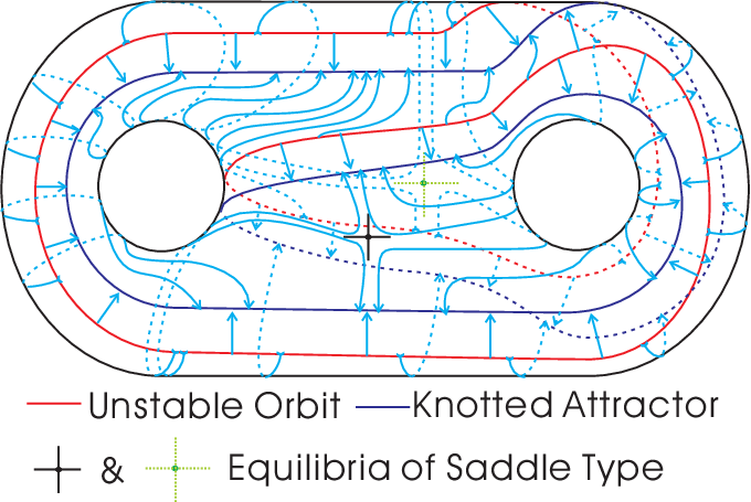
Under the existence of inversely unstable orbit, chaotic behaviour will occur within the invariant set (see fig (20)).

6 Conclusion
We have studied dynamical systems on a genus- surface and extend the generalized automorphic functions (see [Banks & Song, 2006]) to define a general form for these systems (both analytic and non-analytic). Also we look at the topology of knotted attractors under the existence of unstable periodic orbits and prove that for a genus- surface with only one unstable cycle, the number of invariant sets may vary while a maximum of must not be exceeded. Moreover, we extend the result in [Martins, 2004] and show that for a higher genus surface, the individual attractor is not homeomorphic to a circle if there exists an inversely unstable solution within itself. This is purely because of the property of inversely unstable solution which can generate a local behaviour to make the dynamics fight against the effect of global unstable orbit.
In the future paper, we will consider automorphic functions in 3-dimension which will give us systems naturally defined on genus- solid 3-manifolds.
References
- [1] Banks, S. P. “Three-dimensional stratifications, knots and bifurcations of two-dimensional dynamical systems”, Int. J. of Bifurcation and Chaos, Vol. 12, No. 1 (2002) 1-21.
- [2] Banks, S. P. and Song, Y. “Elliptic and automorphic dynamical systems on surfaces”, Int. J. of Bifurcation and Chaos, Vol. 16, No. 4 (2006) 911-923.
- [3] Bowen, R. “On axiom A diffeomorphisms”, AMS, Providence, RT., 1978.
- [4] Ford, L. R. “Automorphic functions”, McGraw–Hill, 1929
- [5] Levinson, N. “Transformation theory of non-linear differential equations of the second order”, The Annals of Mathematics, 2nd Ser., Vol. 45, No. 4. (Oct., 1944), 723-737.
- [6] Manning, A. “There are no new Anosov diffeomeophisms on tori”, Amer. J. Math., 96 (1974), 422.
- [7] Martins, R. “The effect of inversely unstable solutions on the attractor of the forced pendulum equation with friction”, J. of Differential Equations, Vol. 212, Issue 2, 15 May 2005, 351-365.
- [8] Richeson, D. and Wiseman, J. “Bounded homeomorphisms of the open annulus”, New York J. Math. 9 (2003) 55-68.
- [9] Smale, S. “Differentiable dynamical systems”, Bull. Amer. Math. Soc., 73 (1967), 747.
- [10] Wiggins, S. “Global bifurcations and chaos: Analytic methods”, Applied math. Sciences, (1988), New York: Springer–Verlag.