Magnetorotational collapse of very massive stars to black holes in full general relativity
Abstract
We perform axisymmetric simulations of the magnetorotational collapse of very massive stars in full general relativity. Our simulations are applicable to the collapse of supermassive stars with masses and to very massive Population III stars. We model our initial configurations by polytropes, uniformly rotating near the mass-shedding limit and at the onset of radial instability to collapse. The ratio of magnetic to rotational kinetic energy in these configurations is chosen to be small (1% and 10%). We find that such magnetic fields do not affect the initial collapse significantly. The core collapses to a black hole, after which black hole excision is employed to continue the evolution long enough for the hole to reach a quasi-stationary state. We find that the black hole mass is and its spin parameter is , with the remaining matter forming a torus around the black hole. The subsequent evolution of the torus depends on the strength of the magnetic field. We freeze the spacetime metric (“Cowling approximation”) and continue to follow the evolution of the torus after the black hole has relaxed to quasi-stationary equilibrium. In the absence of magnetic fields, the torus settles down following ejection of a small amount of matter due to shock heating. When magnetic fields are present, the field lines gradually collimate along the hole’s rotation axis. MHD shocks and the magnetorotational instability (MRI) generate MHD turbulence in the torus and stochastic accretion onto the central black hole. When the magnetic field is strong, a wind is generated in the torus, and the torus undergoes radial oscillations that drive episodic accretion onto the hole. These oscillations produce long-wavelength gravitational waves potentially detectable by the Laser Interferometer Space Antenna (LISA). The final state of the magnetorotational collapse always consists of a central black hole surrounded by a collimated magnetic field and a hot, thick accretion torus. This system is a viable candidate for the central engine of a long-soft gamma-ray burst.
pacs
04.25.Dm,97.20.Wt,97.60.-sI Introduction
Population III stars born with zero metallicity comprise the first generation of stars. It is believed that their formation causes the reionization of the universe and terminates the “dark ages” (see, e.g., lb01 and references therein). The disruption of Pop III stars following nuclear burning may be responsible for the small metal abundance observed in later generations of stars (e.g. Pop II stars). Simulations of the collapse of primordial molecular clouds suggest that Pop III stars tend to be massive. Masses in the range between and are not uncommon PopIII-mass. Some of these calculations suggest that the initial mass function for Pop III stars has a bimodal distribution, with peaks at and – nu01. Stars with masses between and encounter a pair instability and are likely to be completely disrupted by nuclear-powered explosions hw02. The recent observation of the peculiar Type IIn supernova SN2006gy in NGC1260 points to the possibility that such a disruption can occur in a massive star () even during the current epoch lum-SN. For stars with masses above , the explosive nuclear burning is unable to reverse the implosion and the stars are likely to collapse directly to black holes hw02.
Growing evidence indicates that supermassive black holes (SMBHs) with masses in the range exist and are the engines that power active galactic nuclei (AGNs) and quasars rees1; rees. There is also ample evidence that SMBHs reside at the centers of many, and perhaps most, galaxies richstone, including the Milky Way genzel. The highest redshift of a quasar discovered to date is , corresponding to QSO SDSS 1148+5251 fan03. Accordingly, if they are the energy sources in quasars (QSOs), the first SMBHs must have formed prior to , or within Gyr after the Big Bang in the concordance CDM cosmological model. This requirement sets a significant constraint on black hole seed formation and growth mechanisms in the early universe. Once formed, black holes grow by a combination of mergers and gas accretion.
The more massive the initial seed, the less time is required for it to grow to SMBH scale and the easier it is to have a SMBH in place by . One possible progenitor that readily produces a SMBH is a supermassive star (SMS) with rees1; s03. SMSs can form when gaseous structures build up sufficient radiation pressure to inhibit fragmentation and prevent normal star formation; plausible cosmological scenarios have been proposed that can lead to this situation g01. Alternatively, the seed black holes that later grow to become SMBHs may originate from the collapse of Pop III stars madau. To achieve the required growth to by , it may be necessary for gas accretion, if restricted by the Eddington limiting luminosity, to occur at low efficiency of rest-mass to radiation conversion (). Recent relativistic simulations accretion_disks; gsm04; dv05 show that accretion onto a rotating black hole that has reached spin equilibrium does occur at low efficiency in a magnetized disk with turbulence driven by the magnetorotational instability (MRI) MRI0; MRI; MRIrev. Such accretion may enable a Pop III seed to achieve the necessary growth by s05. But it may be more difficult to use the Pop III seeds to explain the origin of the first generation of the SMBHs should quasars be detected at redshifts significantly higher than .
Recent simulations of binary black hole mergers suggest that gravitational radiation reaction can induce a large kick velocity ( km/s) in the remnants following mergers GW_kick. These large kick velocities may pose a great hazard for the growth of black hole seeds to SMBHs by v07, but such large kicks are possible only if the spins of the black hole binary companions are appreciable and their masses are comparable. Determining the spins of the seed black holes formed from collapse and tracking their subsequent evolution via accretion and minor mergers hb03; gsm04 is therefore important for estimating the kick velocities following major mergers.
It is very likely that massive Pop III and SMSs are rotating and have magnetic fields. A SMS does not reach sufficiently high temperature for nuclear burning to become important before the onset of the general relativistic radial instability bs99. Quasistatic contraction driven by radiative cooling will spin up the star to the mass-shedding limit, provided that viscosity and/or magnetic fields are sufficient to maintain uniform rotation bs99. The star will then evolve secularly along the mass-shedding limit, simultaneously emitting electromagnetic radiation, matter, and angular momentum (see, e.g. zn; sms; bs99). After reaching the onset of radial instability, the star collapses on a dynamical timescale. During the collapse, the rotation becomes differential and the rotational and magnetic energies are both amplified. The black hole that forms will be rotating and surrounded by a magnetized accretion disk. A qualitatively similar final fate should characterize a massive Pop III star .
Shibata and Shapiro performed the first full general relativistic (GR) simulation of the collapse of a very massive, rotating star ss02. They modeled the massive star as a uniformly rotating polytrope spinning at the mass-shedding limit at the onset of radial instability. A massive star is supported largely by thermal radiation pressure and is adequately modeled by an polytrope. They terminated their simulation soon after the black hole formed because of numerical inaccuracies associated with the spacetime singularity that inevitably forms inside the black hole. They estimated the final state of the system using semi-analytic methods (see also ss02b; s04). They concluded that, independent of the initial mass of the progenitor star, the mass of the black hole that forms is and the hole spin parameter is . The remaining gas forms a rotating torus around the nascent black hole.
In this paper, we first repeat the full GR (axisymmetric) simulation performed by Shibata and Shapiro of massive star collapse to the appearance of a black hole. We then employ the technique of black hole excision excision; excision_hydro to continue the evolution. We are able to follow the spacetime evolution for another by this means. By this time, the central black hole and the spacetime metric have both settled down to a quasi-stationary state. We find that the mass and spin parameter of the final black hole are and . These results are close to the semi-analytic estimates in ss02; ss02b; s04. The torus surrounding the black hole continues to evolve long after the black hole has settled down. In order to study the subsequent evolution of the torus, we adopt the “Cowling approximation” whereby we freeze the metric at after the excision and continue to evolve the system for another . We find that a small amount of material () is ejected from the system due to shock heating, and the torus relaxes to a dynamical equilibrium state after the formation of the central black hole.
Next, to study the important role of magnetic fields, we add a small, seed poloidal magnetic field to the initial rotating star and follow the collapse once again. We consider two different strengths of the seed magnetic fields (models S1 and S2). The initial magnetic energy is 1% of the initial rotational kinetic energy for model S1, and 10% of for model S2. Since , we have in both models, where is the gravitational potential energy. Hence in both cases the magnetic fields represent small perturbations to the dynamics of the initial star. During the collapse, the frozen-in poloidal field is amplified as a result of compression. The development of differential rotation generates a toroidal field due to magnetic winding. However, we find that magnetic fields do not affect the collapse significantly before the formation of the central black hole. The final mass and spin parameter of the black hole are about the same as in the unmagnetized case. But magnetic fields do affect the evolution of the torus significantly. Magnetic fields intensify the outflow of the ejected material. The outflow also lasts longer than in the unmagnetized case. As the torus evolves, magnetic fields are collimated along the black hole’s rotation axis. For model S1, MHD shocks and the MRI in the torus create turbulence, which leads to stochastic accretion of material from the torus to the central black hole. For model S2, a strong wind is generated (possibly by the magneto-centrifugal mechanism magnetocen) during the period – following central black hole formation. This wind induces a radial oscillation of the torus, which leads to episodic accretion of material to the central black hole, and long-wavelength gravitational radiation potentially detectable by the Laser Interferometer Space Antenna (LISA).
The final state of the magnetorotational collapse consists of a central black hole surrounded by a collimated magnetic field and a massive, hot, accretion torus. These features provide the essential ingredients for generating ultrarelativistic jets at large distance. Our simple equation of state (EOS) is a reasonable approximation for the collapse of SMSs, but our omission of neutrino emission and other microphysics is certainly not adequate to capture all of the physical processes occurring during the collapse of massive Pop III and Pop I/II stars. Nevertheless, we expect that the black hole-torus remnant that we find will be qualitatively similar to the remnants formed from these progenitors if they are rotating rapidly at the onset of collapse. The reason is that these stars may also be crudely modeled by polytropes initially and their EOSs may also be represented by an adiabatic law during collapse (see s04).
Our simulations may also help explain the formation of the central engine in the collapsar model mw99 of long-soft gamma-ray bursts (GRBs). In addition, some GRBs observed at very high redshift might be related to the gravitational collapse of very massive Pop III stars PopIII-GRB. Hence our simulations may also provide insights into the formation of GRB central engines arising from these stars.
The reminder of this paper is organized as follows. In Sec. II, we briefly describe the mathematical formulation of the Einstein-Maxwell-MHD coupled equations and numerical techniques used to solve them. We then describe our initial data and computational setup in Sec. III. We present our numerical results in Sec. IV and provide a summary of our simulations in Sec. V. Throughout this paper, we adopt geometrical units in which , where and denote the gravitational constant and speed of light, respectively. Cartesian coordinates are denoted by . The coordinates are oriented so that the rotation axis is along the -direction. We define the coordinate radius , cylindrical radius , and azimuthal angle . Coordinate time is denoted by . Greek indices denote spacetime components (), small Latin indices denote spatial components (, and ).
II Formulation
II.1 Basic equations and numerical methods
The formulation and numerical scheme for our GRMHD simulations are the same as those reported in DLSS, to which the reader may refer for details. Here we briefly summarize the method and introduce our notation.
We use the 3+1 formulation of general relativity and decompose the metric into the following form:
| (1) |
The fundamental variables for the metric evolution are the spatial three-metric and extrinsic curvature . We adopt the Baumgarte-Shapiro-Shibata-Nakamura (BSSN) formalism BSSN to evolve and . In this formalism, the evolution variables are the conformal exponent , the conformal 3-metric , three auxiliary functions , the trace of the extrinsic curvature , and the tracefree part of the conformal extrinsic curvature . Here, . The full spacetime metric is related to the three-metric by , where the future-directed, timelike unit vector normal to the time slice can be written in terms of the lapse and shift as .
The Einstein equations are solved in Cartesian coordinates. In this paper, we assume both equatorial and axisymmetry so we only evolve the region with and . We adopt the Cartoon method cartoon to impose axisymmetry in the metric evolution, and use a cylindrical grid to evolve the MHD and Maxwell equations. As for the gauge conditions, we adopt the hyperbolic driver conditions as in excision_hydro to evolve the lapse and shift .
The fundamental variables in ideal MHD are the rest-mass density , specific internal energy , pressure , four-velocity , and magnetic field measured by a normal observer moving with a 4-velocity (note that ). The ideal MHD condition is written as , where is the electromagnetic tensor. The tensor and its dual in the ideal MHD approximation are given by
| (2) | |||
| (3) |
where is the Levi-Civita tensor. Here we have introduced an auxiliary magnetic 4-vector , where is the magnetic field measured by an observer comoving with the fluid and is related to by
| (4) |
The energy-momentum tensor is written as
| (5) |
where and denote the fluid and electromagnetic pieces of the stress-energy tensor. They are given by
| (6) | |||
| (7) |
where is the specific enthalpy, and . Hence, the total stress-energy tensor becomes
| (8) |
In our numerical implementation of the GRMHD and magnetic induction equations, we evolve the densitized density , densitized momentum density , densitized energy density , and densitized magnetic field . They are defined as
| (9) | |||
| (10) | |||
| (11) | |||
| (12) |
During the evolution, we also need the three-velocity .
The GRMHD and induction equations are written in conservative form for variables , , , and and evolved using a high-resolution shock-capturing (HRSC) scheme. Specifically, we use the monotonized central (MC) scheme vL77 for data reconstruction and the HLL (Harten, Lax and van-Leer) scheme HLL to compute the flux. The magnetic field has to satisfy the no monopole constraint . We adopt the flux-interpolated constrained transport (flux-CT) scheme t00 to impose this constraint. This scheme guarantees that no magnetic monopoles will be created in the computational grid during numerical evolution. At each timestep, the primitive variables must be computed from the evolution variables . This is done by numerically solving the algebraic equations (9)–(11) together with an EOS .
As in many hydrodynamic simulations in astrophysics, we add a tenuous “atmosphere” that covers the computational grid outside the star. The atmospheric rest-mass density is set to before the black hole forms, where is the initial rest-mass central density of the star. In the excision evolution where the system consists of a central black hole and a surrounding torus, the maximum density in the torus is , and we set the atmosphere density to .
The codes used here have been tested in multiple relativistic MHD simulations, including MHD shocks, nonlinear MHD wave propagation, magnetized Bondi accretion, and MHD waves induced by linear gravitational waves DLSS. We have also compared this code with the GRMHD code developed independently by Shibata and Sekiguchi SS05 by performing simulations of the evolution of magnetized, differentially rotating, relativistic, hypermassive neutron stars DLSSS; DLSSS2, and of magnetorotational collapse of stellar cores SLSS. We obtain good agreement between these two independent codes.
II.2 Equation of state
In this paper, we adopt the simple () polytropic EOS to construct the initial model and (-law EOS) during the evolution. This EOS is a good approximation for the pre-collapse core of a massive Pop III star bac84 or the bulk of a SMS zn; st83, where pressure is dominated by thermal radiation. For a Pop I/II star, which has smaller mass, the pressure of the pre-collapse core is dominated by the relativistic degenerate electron pressure, which is also well-approximated by a EOS. During the collapse, the EOS stiffens when the density exceeds nuclear density . However, if the mass of the collapsing core exceeds a critical value , the black hole horizon appears before the star reaches the nuclear density. In this case, the stiffening of the EOS has no effect on the collapse. To estimate , consider the collapse of a uniform density dust sphere (Oppenheimer-Snyder collapse). A horizon appears when the areal radius of the sphere reaches . At this time, the density is . Setting , gives . For a SMS, the mass is much larger than . For a Pop III star of mass , the mass of the collapsing core is hw02, which is still much larger than . Hence the EOS is also a good approximation during the entire collapse phase for very massive Pop III stars. For Pop I/II stars, on the other hand, the core mass is less than and a more realistic EOS is required in the late stages. In addition, neutrino emission and transport are also important to the dynamics of the collapse for these stars. Neutrino generation and transport also play a role in the collapse of Pop III stars hw02; stks07, but are probably not dynamically important for the most massive progenitors or for SMSs because of their low temperature and density.
II.3 Diagnostics
During the evolution, we monitor the L2 norm of the Hamiltonian and momentum constraints as in DLSSS2. We find the violation of the constraints is at most a few percent before excision. After the excision, the constraints can rise to %. We terminate the excision evolution before the constraints reach 20%.
We also compute the rest mass , ADM mass and angular momentum during the evolution. They are computed by the following volume integrals:
| (13) | |||||
| (14) | |||||
| (15) | |||||
| (16) |
where is the Christoffel symbol and is the Riemann scalar associated with . Note that the above formula for is only valid in an axisymmetric spacetime Wald. The rest mass is conserved as a result of the baryon number conservation. Angular momentum is conserved in axisymmetry, as gravitational radiation carries no angular momentum. However, is not conserved since gravitational radiation carries energy and propagates off the computational grid. We find that remains constant to within 2%. Our finite difference scheme guarantees that and computed from the above volume integrals are conserved to machine precision provided that no fluid leaves the computational grid. However, we perform several regriddings during the calculation (see Section III) and these leave behind a few percent of and in the outermost layers.
During the excision evolution, we compute the rest mass and angular momentum of the disk outside the black hole by computing integrals (13) and (16) over the volume outside the apparent horizon. The irreducible mass of the black hole is given by , where is the surface area of the apparent horizon. Since is conserved, we can compute the black hole’s angular momentum by
| (17) |
where is the loss of angular momentum as a result of regriddings and matter leaving the grid. The black hole’s mass is then computed from the formula
| (18) |
which is exact for a Kerr spacetime, and is in accord with the formula derived using the isolated and dynamical horizon formalism iso-dyn-hor.
At after the excision evolution, we find that the spacetime becomes nearly stationary. In this case, the energy is approximately conserved thereafter, where
| (19) |
We can then define the fluxes of rest mass, energy, and angular momentum across any closed two-dimensional surface in a time slice:
| (20) | |||
| (21) | |||
| (22) |
where
| (23) |
and is the Levi-Civita tensor associated with the three-metric . If is a sphere of radius , the above expressions reduce to
| (24) | |||
| (25) | |||
| (26) |
where . The total energy flux is very close to the rest-mass flux since is primarily composed of the rest-mass energy flow. Thus, we define another energy flux by subtracting the rest-mass flow: . We note that contains kinetic, thermal, electromagnetic, and gravitational potential energy fluxes. If at sufficiently large radius, an unbound outflow (overcoming gravitational binding energy) is present.
Another method to determine whether a fluid particle is unbound is to compute . In a stationary spacetime, the value of of a particle moving on a geodesic is conserved. If the particle is unbound, the radial velocity and at infinity. Hence and are useful diagnostics to determine if the fluid element is unbound, provided that the fluid motion is predominantly ballistic and pressure and electromagnetic forces can be neglected. This is usually the case in the low-density region.
During the excision evolution, the MRI may develop in the torus surrounding the central black hole. The growth time (-folding time) and wavelength of the fastest-growing MRI mode can be roughly estimated by the following formulae derived in linear perturbation theory in Newtonian gravitation MRIrev; SLSS:
| (27) | |||||
| (28) |
where is angular velocity, is the -component of the Alfvén speed and
| (29) |
is the epicyclic frequency.
III Initial Data and Grid setup
III.1 Initial Data
We model the pre-collapse star as a uniformly rotating star satisfying the polytropic EOS . We set in our code. As explained in cst92, our result can be scaled to arbitrary values of or, equivalently, the ADM mass ; only nondimensional ratios are invariant. For example, , , ,… etc.
We use the same initial model as in ss02, whereby the star is rotating near the mass-shedding limit with . The equatorial radius of the star is km. This is the configuration where the polytrope is on the verge of radial instability against gravitational collapse due to general relativity bs99. The central density of the star is . For a SMS with mass , this general relativistic instability triggers the collapse, as opposed to microphysical processes such as pair instability.
We add a small amount of poloidal seed magnetic field to this equilibrium star, employing a magnetic vector potential of the form
| (30) |
where , and is a constant that determines the strength of the initial magnetic field. The magnetic field is computed by the formula . A similar form of the initial magnetic field has been used in the study of magnetized accretion disks around a stationary black hole accretion_disks; dvhk03, the collapse of hypermassive neutron stars DLSSS; DLSSS2 and the collapse of a magnetized, stellar core of a high mass star SLSS. We choose two nonzero values of the constants so that the values of initial magnetic energy
| (31) |
are 1% and 10% of the initial rotational kinetic energy (corresponding to and ). Hence adding this seed magnetic field causes only a slight perturbation to the star. We label these two models as S1 and S2, respectively. We also study the unmagnetized case (, model S0) to compare with the previous result reported in ss02. We can also characterize the strength of the magnetic field by the volume-averaged ratio of gas pressure to the magnetic pressure. Specifically, we define , where the magnetic pressure is and
Here is the proper volume element and is the volume of the star. This definition of is used in dvhk03 in the study of magnetized accretion disks around central black holes. The value of for models S1 and S2 are 3700 and 370, respectively. We also define the averaged strength of magnetic field by . In cgs units, we find
for model S1 and
for model S2.
The strength of the magnetic field inside a Pop III star is unknown and is currently not addressed by theoretical models dealing with their cosmological formation abn02. Our goal is to determine what effects, if any, magnetic fields may have on the eventual collapse of the stars to black holes. After all, they are possible progenitors of GRBs, and many GRB models require a magnetized disk around a black hole. Here, we choose the strengths of the seed magnetic field to be sufficiently large for us to perform reliable simulations with limited computational resources and still be able to resolve the wavelength of the fastest growing MRI mode. We note that these magnetic field strengths are still quite small dynamically (small and large ), and so the magnetic field does not affect the dynamics of the collapse (see Sec. IV). However, the post-collapse evolution does depend on the chosen strengths. In Sec IV, we will discuss how our results may change for even smaller field strengths.
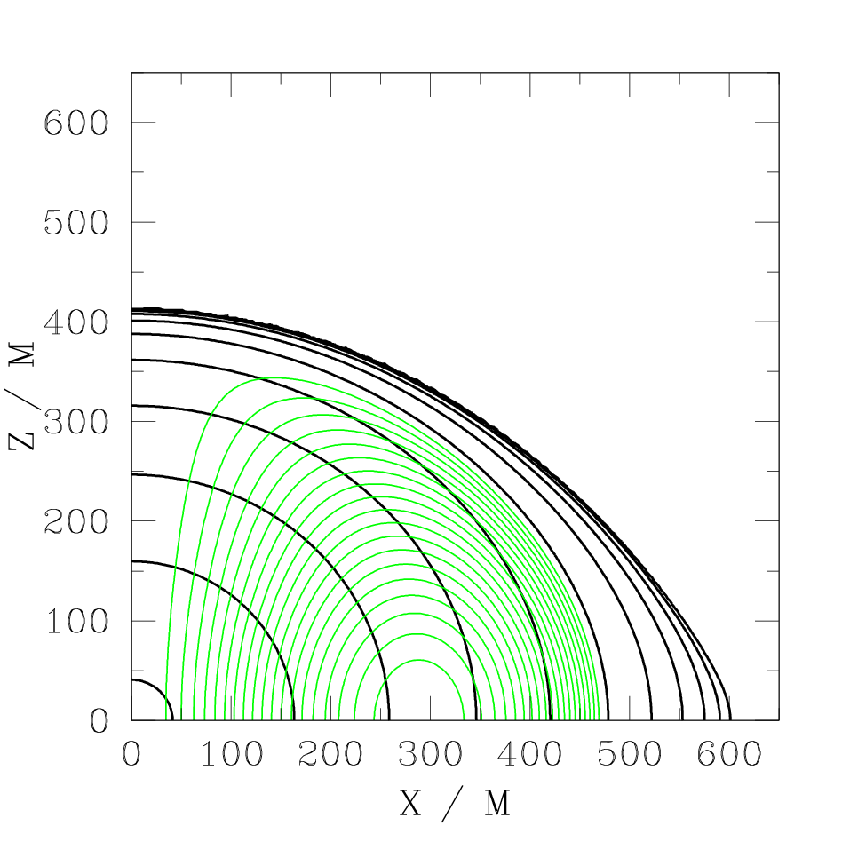
Following ss02, we induce collapse by depleting 1% of the pressure (i.e., ) everywhere inside the star. The parameters of our models are summarized in Table 1. The density and magnetic field profiles of our pre-collapse model are shown in Figure 1.
| Model | |||
|---|---|---|---|
| S0 | 0 | 0 | 0 |
| S1 | 0.01 | 3700 | G |
| S2 | 0.10 | 370 | G |
III.2 Grid Setup
We perform simulations using a cell-centered uniform grid with size in --, covering a computational domain , , and . Here, and are constants and . The variables in the planes are computed from the quantities in the plane by imposing axisymmetry. Since the characteristic radius of the star decreases by a factor of during the collapse (from to ), using a fixed uniform grid with sufficient resolution for the entire collapse phase is computationally prohibitive. In order to save computational resources and at the same time ensure adequate resolution throughout the simulation, we adopt a regridding technique similar to the algorithm described in ss02. When gravity is weak (in the Newtonian regime), the characteristic radius of the star is proportional to , where is the central lapse. We thus use a regridding algorithm based on the values of . During the early stages, the collapse proceeds in a homologous manner. We set and when . Keeping fixed, we decreases as the collapse proceeds: when , when . After this stage, the collapse in the core is faster than in the outer layers. We increase the grid number and decrease as follows: and when , and when . In the last stage, the star collapses to a black hole. In order to allocate our grid more effectively in this last stage, we interpolated the data onto a multiple-transition fisheye coordinates fisheye when .
The multiple transition fisheye coordinates are related to the original coordinates through the following transformation:
| (32) | |||||
| (33) | |||||
| (34) |
where , , , , and are constant parameters. In the last stage of collapse (), we use a cell-centered uniform grid with in fisheye coordinates with parameters , , , , and . When transformed back to the original coordinate system, the outer boundary is and the resolutions are
| (35) |
We find that the total rest mass and angular momentum that are discarded as a result of the regriddings are about 1% and 5–8% of their initial values for the models considered.
IV Results


Figure 2 shows the evolution of central density and lapse for the three models. Figures 3–5 show the density contours and velocity vectors during pre-excision evolution for models S0, S1 and S2 respectively. Poloidal magnetic field lines are also shown for models S1 and S2 in Figs. 4 and 5. We see that magnetic fields slightly slow down the collapse. As mentioned in Sec. III, the collapse proceeds in a homologous manner at the beginning. When the central lapse decreases to , the central region collapses faster than the outer layers. The apparent horizon appears at for model S0, for S1 and for S2. Without excision, the code becomes inaccurate soon after the formation of the apparent horizon because of the grid stretching.


To continue the evolution, we excise a spherical region inside the apparent horizon. We start the excision evolution a few after the apparent horizon forms. We are able to follow the evolution reliably for another , after which the Hamiltonian and momentum constraints increase substantially. This eventual breakdown is probably because the metric inside the horizon, which is not computed accurately, slowly leaks out to the region outside due to superluminal gauge modes. We are currently investigating other gauge conditions, as well as other techniques to overcome the numerical difficulty. As the collapse proceeds, the mass and angular momentum of the central black hole increase before settling down to quasi-stationary values. Figures 6–8 show the post-excision evolution of the black hole’s irreducible mass , mass , spin parameter , and the rest mass of the material outside the apparent horizon , for the three models. We see that after , the black hole settles down to a quasi-stationary state, with and for all the three models. This result agrees roughly with our earlier simulations and analytic estimates for unmagnetized collapse ( and ) in ss02; ss02b; s04. The remaining material, having too much angular momentum, forms a torus surrounding the black hole (see Figs. 9–11). Even though the central black hole has settled down after , the torus continues to evolve as material from the outer layers gradually reaches the central region. The dynamical timescale at radius is . Hence at , and at . Since the torus extends beyond , we need to follow the evolution for at least . To study the subsequent evolution, we adopt the Cowling approximation by freezing the metric at , where is the time when excision starts. This is a fairly good approximation since the material outside the horizon contributes only of the total mass and so the metric is dominated by the central black hole, which has settled down. We have compared the results of our Cowling (stationary metric) and non-Cowling (dynamic metric) runs during the transition interval and find good agreement.


Figure 9 shows snapshots of density contours and velocity fields for model S0 in the post-excision evolution. We terminate the simulation at , where most of the dynamical processes have ended. We find that an outflow develops at near the horizon and becomes prominent at . The outflow is due to the fact that material from the outer layers arrives into the inner region with a substantial amount of angular momentum. When it reaches the inner region, the centrifugal barrier prevents it from falling into the black hole. The fluid particles move with “zoom-whirl”-like trajectories zoom-whirl and accumulate near the black hole. As more fluid particles arrive and smash into interior layers, the fluid heats up and forms a shock, which propagates outward and creates an outflow along the surface of the torus. While this outflow is still expanding, we find that a secondary, weaker outflow forms at , which can be seen in the second and third plots in Fig. 9. A few more episodes of smaller outflow develop as more material from the outer layers arrive. However, the process damps by by which time most of the material has reached the central region and the residual infalling fluid does not have enough momentum to push on the torus and generate further outflow. To determine if the outflowing material is unbound, we calculate the quantity . As discussed in Sec. II, any unbound fluid particle moving in a low density region (in which pressure and electromagnetic forces are negligible) has . We find that the outflow material is indeed unbound, but the total rest mass of the unbound fluid is only . The outflow reaches the outer boundary of our grid () after . Most of the unbound material leaves the grid after . During this same time, the infalling material in the outer region of the torus close to the equatorial plane also rebounds outward because of the centrifugal barrier. We have checked that this outward moving fluid remains bound (), but about of rest mass leaves the grid by the time we terminate our simulation at . This outward moving fluid has too much angular momentum to be able to remain in the inner region. The torus in the inner region with settles down to quasi-equilibrium by .
Figures 10 and 11 show snapshots of density contours, velocity fields and poloidal magnetic field lines for models S1 and S2 in the post-excision evolution. We find similar outflow as in the case S0, but the outflow in S2 develops at time , much earlier than that in S0. Unlike S0, the outflow in S1 and S2 is generated continuously rather than intermittently. The outflow is stronger than S0 and about of the rest mass becomes unbound for S1 and for S2, much larger than the case of S0. In the presence of magnetic fields, the outflow carries the frozen magnetic field and travels outward along the torus’s surface. This causes the field lines near the boundary of the outflow and torus to bend (see Figs. 10 and 11). This bending amplifies the magnetic field in that region and hence the outflow is intensified by the extra magnetic pressure. A magnetic shock is also generated in the region, which leads to turbulence in the torus. The bending is more significant in S1 than in S2. This is because in S2, the magnetic field is strong enough to quickly counteract the bending and drives more fluid outward. Figure 12 shows the rest-mass flux , energy flux and angular momentum flux through a spherical surface of radius for the three models. We see that the outflow is significantly stronger in the presence of magnetic fields. Figure 12 also indicates that a sustained flux is present in the time period – for model S2. We find that this flux is not due to outflow generated near the black hole, but due to a wind that arises in the middle of the torus. We find that in the wind the fluid moves along the magnetic field lines. The inclination angle between the field lines and -axis is between and . This suggests that the wind is driven by the magneto-centrifugal mechanism magnetocen. The outflows in models S1 and S2 cause the field lines to collimate along the rotation axis of the black hole. For model S2, the outflow and the subsequent wind carry away a substantial amount of magnetic energy from the torus. At , the wind subsides and the interior of the remaining torus has a weak magnetic field. The outflow and wind in model S2 are so strong that they perturb the equilibrium of the inner torus and causes it to oscillate radially. As in the case of S0, there is bound fluid moving out of the grid as a result of centrifugal bounce in models S1 and S2. By the end of the simulation (), only 0.04M of the rest mass remains in the inner torus in model S1 and remains in model S2.

Figure 13 shows the rest-mass flux through the apparent horizon for the three models. For model S0, the inward flux decreases with time as the torus settles down to dynamical equilibrium. Without magnetic fields or viscosity, there is no dissipation to drive further accretion. For model S1, we see that at late time () material from the torus accretes into the central black hole in a stochastic manner. Stochastic accretion is often seen in simulations of magnetized accretion disks around stationary black holes (see e.g. dvhk03; mhd-disk). This suggests that the accretion is due to magnetic-induced turbulence in the torus. The turbulence is generated initially by the magnetic shock as a result of the outflow, and is then sustained by the MRI. To verify that we are able to resolve the MRI, we compute the wavelength of the fastest growing MRI mode using Eq. (28). We find that 15 in some region near the equatorial plane, where is our grid spacing. This suggests that the MRI can be resolved in our simulation. For model S2, the radial oscillation of the inner torus causes episodic accretion into the central black hole. When the torus swings away from the black hole, no accretion occurs. Accretion resumes when the torus swings towards the black hole. This explains the episodic mass accretion pattern seen in Fig. 13. The small accretion rate in the figure is due to accretion from the atmosphere.
When the magnetic field strength is much smaller than that in S1, we expect the dynamics of the fluid evolution to be very similar to S0 initially. As in the case of S1 and S2, the outflow is expected to collimate the magnetic field lines and generate magnetic shocks which may create turbulence in the torus. Turbulence can also be generated by the MRI, which operates on the orbital timescale of the torus independent of the field strength. We should then expect to see the stochastic accretion similar to the case in S1. Both a collimated magnetic field and a massive, accretion torus surrounding a central black hole are essential ingredients for launching ultrarelativistic jets jet-launching. The black hole-torus system observed in our simulations provides a viable central engine for long-soft GRBs.
The radial oscillation observed in model S2 gives rise to gravitational radiation. The oscillation period of corresponds to the gravitational wave frequency Hz at redshift . For a SMS with , the signal is in the LISA frequency band. To estimate its amplitude, we apply the quadrupole formula , where is the source’s luminosity distance, – is the tracefree quadrupole moment and . Here is the characteristic radius of the torus and is the amplitude of the oscillation. Setting and , we obtain
| (36) |
where Gpc corresponds to redshift in the concordance CDM cosmology model with , and wmap. We note that if the signal can be tracked for cycles, where is expected to be a few, the effective wave strength will be increased by a factor of . Such a gravitational wave signal may be detectable by LISA [see lisa-sen for LISA’s sensitivity curve].
Our simulations are adiabatic and do not take into account the heat loss due to neutrino cooling. To determine if this effect can be neglected during the phase in which the torus forms and evolves around the black hole, we estimate the neutrino cooling timescale. We first compute the temperature in the disk from the specific thermal energy density , where for our adopted EOS. We find from our data that the typical values of and in the disk at late times are
| (37) | |||||
| (38) |
where we have restored the speed of light in the above equation. To calculate the temperature , we adopt the expression of in pwf99:
| (39) |
where is the Boltzmann constant, is radiation constant, is proton mass, and is the mass fraction of free nucleons approximately given by qw96 . Here and . The first term in Eq. (39) is the specific thermal energy density of an ideal gas, and the second term is the contribution from thermal radiation. The quantity is a temperature-dependent numerical factor depending on the species of ultrarelativistic particles that contribute to thermal radiation. When , photons, ultra-relativistic electrons and positrons are present (assuming thermal neutrinos are negligible) and . On the other hand, when , only photons contribute to thermal radiation and . Combining Eqs. (37)–(39), we obtain
| (40) |
where . For , we find and, not surprisingly, is dominated by thermal photon radiation. At this density and temperature, the torus is optically thin to neutrinos. The cooling rate is dominated by the pair neutrino process and the value is itoh89. The neutrino cooling timescale is , which is much longer than the timescale in our simulations (). Even for , we find . The same conclusion (i.e. ) holds for all . Hence neutrino cooling can be neglected in the torus evolution.
V Summary and conclusion
In this paper, we study the magnetorotational collapse of very massive stars by performing full GRMHD simulations in axisymmetry. We model the pre-collapse star by an polytrope uniformly rotating near the mass-shedding limit at the onset of radial collapse. We adopt an adiabatic EOS for the fluid. We study three models, which we label S0, S1 and S2. The three models differ by the strength of the initial magnetic field (see Table 1). Model S0 is unmagnetized (), whereas the ratio of the initial magnetic to kinetic energies () are 1% and 10% for models S1 and S2, respectively.
We find that these magnetic fields do not affect the initial collapse significantly. An apparent horizon forms at time . The black hole grows as the collapse proceeds, and settles down at a time after the formation of the apparent horizon. For all three models we study, we find that the mass and spin parameter of the black hole are approximately and 0.7 respectively, where is the initial mass of the star. These values roughly agree with the semi-analytic estimates in ss02; ss02b; s04. The remaining material forms a torus around the central black hole. Although the central black hole has settled down to quasi-stationary equilibrium, the ambient torus continues to evolve as fluid from the outer layers of the star gradually reaches the central region. During this epoch, magnetic fields have substantial influence on the evolution of the torus. The infalling fluid particles have large angular momenta. They pile up near the black hole horizon, are heated by shocks and then get ejected along the surface of the torus, forming an unbound outflow. In the presence of magnetic fields, the outflow bends the magnetic field lines near the boundary of the outflow, which amplifies the field and induces magnetic shocks. The extra magnetic pressure makes the outflow stronger than in the unmagnetized case. The outflow also causes the magnetic fields to collimate along the black hole’s rotation axis. For model S0, when the outflow leaves the central region, the torus settles down to equilibrium. For model S1, MHD turbulence generated by magnetic shocks and MRI in the disk causes stochastic accretion of material into the black hole. For model S2, when the outflow leaves, strong magnetic fields in the torus create a magnetic wind, driving more material and magnetic field out of the torus. During this time, the torus acquires a quasiperiodic radial oscillation. The wind subsides as the magnetic field inside the torus decreases. The radial oscillations of the torus induce episodic accretion of material into the central black hole. The oscillations also generate gravitational radiation, which might be detectable by LISA at redshift if the mass of the star satisfies .
If the initial magnetic field strength is smaller than that in model S1, we expect the evolution to be similar to S1. In particular, the evolution in the collapse phase should remain unchanged. We also expect the outflow to collimate the magnetic field lines and generate magnetic shocks, which then leads to turbulence in the disk. Turbulence will be maintained as a result of the MRI. We thus expect stochastic accretion of the torus as in the case of S1.
In typical cases, the final stage of the magnetorotational collapse consists of a central black hole surrounded by a collimated magnetic field and a massive torus. These are the main ingredients for generating ultrarelativistic jets at large distance from the central source. The final system obtained in our simulations is thus capable of generating a long-soft GRB. In principle, the collapse of a very massive star could result in the simultaneous detection of gravitational waves and a GRB. The gravitational wave signal consists of an initial burst signal due to collapse, a black-hole ring-down signal, and a quasi-periodic signal due to the torus’s oscillation if the magnetic field is strong.
A few issues warrant further study. The first is the EOS. Our adiabatic EOS is a good approximation only for very massive stars. But most of the observed long-soft GRBs are believed to be triggered by the magnetorotational core collapse of smaller-mass Pop I/II stars mw99. The core mass of a Pop I/II star is less than . A EOS describes the early phase of core collapse in such a star, when the pressure is dominated by relativistic degenerate electrons. But the EOS stiffens when the core density exceeds nuclear density and this happens before an apparent horizon forms. Also, a realistic EOS for this scenario must incorporate more detailed microphysics and neutrino transport.
A second issue concerns a search for a more robust singularity-avoiding algorithm once a black hole forms. As mentioned in Sec. IV, we are only able to evolve the system for after the black hole formation with our current excision technique. However, the evolution timescale of the torus is . While this evolution could be reliably tracked in the Cowling approximation, we are interested in more general scenarios. We plan to explore this issue in two ways. The first will be to search for better lapse and shift conditions that can suppress troublesome superluminal gauge modes. The other will be to identify a gauge that can drive the metric inside the horizon to a puncture-like solution, a technique which has been used with great success in binary black hole simulations moving-punctures. Simple experimentation with vacuum black holes and black holes immersed in hydrodynamic fluid suggest that there exist such gauge choices fbest07.
The third issue concerns our assumption of axisymmetry. Nonaxisymmetric instabilities such as bar and/or one-armed spiral instabilities may develop during the collapse, which could affect the subsequent dynamics (but see sbss02 for a treatment of unmagnetized collapse in full post-Newtonian gravitation). Additionally, the MHD turbulence developed as a result of magnetic shocks and the MRI will be different. In particular, turbulence arises and persists more readily in due to the lack of symmetry. More specifically, according to the axisymmetric anti-dynamo theorem moffatt78, sustained growth of the magnetic field energy is not possible through axisymmetric turbulence. However, a full GRMHD simulation covering the required dynamic range for massive stellar collapse is computationally challenging and possibly beyond the resources currently available. This is because the torus extends to a large distance away from the central black hole, requiring vast dynamic range, and the dynamical timescale of the torus is very long. Though simulations in full dimensions will eventually be necessary to capture the full behavior of the collapse, the results presented here likely provide a reasonable first approximation.
Acknowledgements.
Numerical computations were performed at the National Center for Supercomputing Applications at the University of Illinois at Urbana-Champaign (UIUC). This work was supported in part by NSF Grants PHY-0205155, PHY-0345151 and PHY-0650377, NASA Grants NNG04GK54G, NNX07AG96G and NNG046N90H at UIUC.References
- (1) A. Loeb, and R. Barkana, Ann. Rev. Astron. & Astrophys., 39, 19 (2001); V. Bromm, and R.B. Larson, Ann. Rev. Astron. & Astrophys., 42, 79 (2004).
- (2) J.P. Ostriker, and N.Y. Gnedin, Astrophys. J. Lett., 472, L63 (1996); V. Bromm, P.S. Coppi, and R.B. Larson, Astrophys. J. Lett., 527, L5 (1999); T. Abel, G.L. Bryan, and M.L. Norman, Astrophys. J., 540, 39 (2000).
- (3) F. Nakamura, and M. Umemura, Astrophys. J., 548, 19 (2001).
- (4) C.L. Fryer, S.E. Woosley, and A. Heger, Astrophys. J., 550, 372 (2001);
- (5) N. Smith etal., submitted to Astrophys. J. (arXiv:astro-ph/0612617v2).
- (6) M.J. Rees, Ann. Rev. Astron. & Astrophys., 22, 471 (1984);
- (7) M.J. Rees, in Black Holes and Relativistic Stars, ed. R.M. Wald (Chicago: Chicago Univ. Press), 79 (1998); M.J. Rees, in Black Holes in Binaries and Galactic Nuclei, ed. L. Kaper, E.P.J. van den Heurel, and P.A. Woudt (New York: Springer-Verlag), 351 (2001); F.D. Macchetto, in Towards a New Millennium in Galaxy Morphology, ed. D.L. Block, I. Puerari, A. Stockton, and D. Ferreira (Dordrecht: Kluwer, 1999); F.D. Macchetto, Astrophys. Space Sci., 269, 269 (1999).
- (8) D. Richstone et al, Nature, 395, A14 (1998); L.C. Ho, in Observational Evidence for Black Holes in the Universe, ed. S.K. Chakrabarti (Dordrecht: Kluwer), 157 (1999).
- (9) R. Genzel, A. Eckart, T. Ott, and F. Eisenhauer, Mon. Not. Royal Astro. Soc., 291, 219 (1997); A.M. Ghez, M. Morris, E.E. Becklin, A. Tanner, and T. Kremenek, Nature, 407, 349 (2000); A.M. Ghez, E. Becklin, G. Duchene, S. Hornstein, M. Morris, S. Salim, and A. Tanner, Astron. Nachr./AN Supp. issue No. 1, 324, 527 (2003); R. Schödel et al., Nature, 419, 694 (2002).
- (10) X. Fan et al, Astron. J., 125, 1649 (2003).
- (11) S.L. Shapiro, in Carnegie Observatories Astrophysics Series, Vol. 1: Coevolution of Black Holes and Galaxies, ed. L. C. Ho (Cambridge Univ. Press: Cambridge), p. 103 (2004).
- (12) O.Y. Gnedin, Class. & Quant. Grav., 18, 3983 (2001); V. Bromm, and A. Loeb, Astrophys. J., 596, 34 (2003).
- (13) P. Madau, and M. Rees, Astrophys. J. Lett, 551, L27 (2001).
- (14) J.C. McKinney, and C.F. Gammie, Astrophys. J., 611, 977 (2004).
- (15) C.F. Gammie, S.L. Shapiro, and J.C. McKinney, Astrophys. J., 602, 312 (2004).
- (16) J-P. De Villiers, J.F. Hawley, J.H. Krolik, and S. Hirose, Astrophys. J., 620, 878 (2005).
- (17) V. P. Velikhov, Soc. Phys. JETP, 36, 995 (1959); S. Chandrasekhar, Proc. Natl. Acad. Sci. USA, 46, 253 (1960).
- (18) S. A. Balbus and J. F. Hawley, Astrophys. J. 376, 214 (1991)
- (19) S. A. Balbus and J. F. Hawley, Rev. Mod. Phys. 70, 1 (1998).
- (20) S.L. Shapiro, Astrophys. J., 620, 59 (2005); M. Volonteri, and M.J. Rees, Astrophys. J., 650, 669 (2006).
- (21) Ya.B. Zeldovich, and I.D. Novikov, Relativistic Astrophysics, University of Chicago Press, Chicago (1971).
- (22) S.L. Shapiro and S.A. Teukolsky, Black Holes, White Dwarfs, and Neutron Stars, Wiley Interscience (New York, 1983).
- (23) F. Herrmann, I. Hinder, D. Shoemaker, P. Laguna, and R.A. Matzner, Astrophys. J., in press (gr-qc/0701143); M. Koppitz, D. Pollney, C. Reisswig, L. Rezzolla, J. Thornburg, P. Diener, and E. Schnetter, gr-qc/0701163; M. Campanelli, C.O. Lousto, Y. Zlochower, and D. Merritt, Astrophys. J., in press (gr-qc/0701164); J.A. Gonzalez, M.D. Hannam, U. Sperhake, B. Brugmann, and S. Husa, gr-qc/0702052; M. Campanelli, C.O. Lousto, Y. Zlochower, and D. Merritt, gr-qc/0702133; W. Tichy, and P. Marronetti, gr-qc/0703075.
- (24) M. Volonteri, submitted to Astrophys. J. Lett. (astro-ph/0703180).
- (25) S.A. Hughes, and R.D. Blandford, Astrophys. J. Lett., 585, L101 (2003).
- (26) T.W. Baumgarte, and S.L. Shapiro, Astrophys. J., 526, 941 (1999).
- (27) G.S. Bisnovatyi-Kogan, Ya.B. Zeldovich, and I.D. Novikov, Soviet Astron., 11, 419 (1967).
- (28) M. Shibata, and S.L. Shapiro, Astrophys. J., 572, L39 (2002).
- (29) S.L. Shapiro, and M. Shibata, Astrophys. J., 577, 904 (2002).
- (30) S.L. Shapiro, Astrophys. J., 610, 913 (2004).
- (31) M. Alcubierre and B. Brügmann, Phys. Rev. D 63, 104006 (2001); H.-J. Yo, T. W. Baumgarte, and S. L. Shapiro, Phys. Rev. D 66, 084026 (2002);
- (32) M. D. Duez, S. L. Shapiro, and H.-J. Yo, Phys. Rev. D 69, 104016 (2004).
- (33) R. D. Blandford and D. G. Payne, Mon. Not. R. Astro. Soc. 199, 883 (1982).
- (34) A. MacFadyen, and S.E. Woosley, Astrophys. J., 524, 262 (1999).
- (35) R. Schneider, D. Guetta, and A. Ferrara, Mon. Not. Roy. Astro. Soc., 334, 173 (2002); V. Bromm, and A. Loeb, Astrophys. J., 642, 382 (2006).
- (36) M. D. Duez, Y. T. Liu, S. L. Shapiro, and B. C. Stephens, Phys. Rev. D 72, 024028 (2005).
- (37) M. Shibata and T. Nakamura, Phys. Rev. D 52, 5428 (1995); T. W. Baumgarte and S. L. Shapiro, Phys. Rev. D 59, 024007 (1998).
- (38) M. Alcubierre, S. Brandt, B. Brügmann, D. Holz, E. Seidel, R. Takahashi and J. Thornburg, Int. J. Mod. Phys. D 10, 273 (2001).
- (39) B. J. van Leer, J. Comput. Phys. 23, 276 (1977).
- (40) A. Harten, P. D. Lax, and B. J. van Leer, SIAM Rev. 25, 35 (1983).
- (41) J.R. Bond, W.D. Arnett, and B.J. Carr, Astrophys. J., 280, 825 (1984).
- (42) G.B. Cook, S.L. Shapiro, and S.A. Teukolsky, Astrophys. J., 398, 203 (1992).
- (43) G. Tóth, J. Comput. Phys. 161, 605 (2000); C.F. Gammie, J.C. McKinney, and G. Tóth, Astrophys. J. 589, 444 (2003).
- (44) M. Shibata and Y.-I. Sekiguchi, Phys. Rev. D 72, 044014 (2005).
- (45) M. D. Duez, Y. T. Liu, S. L. Shapiro, M. Shibata, and B. C. Stephens, Phys. Rev. Lett. 96, 031101 (2006); M. Shibata, M. D. Duez, Y. T. Liu, S. L. Shapiro, and B. C. Stephens, Phys. Rev. Lett. 96, 031102 (2006).
- (46) M. D. Duez, Y. T. Liu, S. L. Shapiro, M. Shibata, and B. C. Stephens, Phys. Rev. D, 73, 104015 (2006).
- (47) M. Shibata, Y.T. Liu, S.L. Shapiro, and B.C. Stephens, Phys. Rev. D, 74, 104026 (2006).
- (48) J-P. De Villiers, J.F. Hawley, and J.H. Krolik, Astrophys. J., 599, 1238 (2003).
- (49) T. Abel, G.L. Bryan, and M.L. Norman, ASP Conference Proceedings, Vol. 285, edited by E.K. Grebel & W. Brandner (San Francisco: Astro. Soc. of the Pacific, 2002).
- (50) Y. Suwa, T. Takiwaki, K. Kotake, and K. Sato, accepted for publication in PASJ (arXiv:0704.1945v1 [astro-ph]).
- (51) R. M. Wald, General Relativity (Univ. of Chicago, Chicago, 1984), p. 297.
- (52) A. Ashtekar, and B. Krishnan, Living Rev. Relativity, 7, 10 (2004) (http://www.livingreviews.org/lrr-2004-10); O. Dreyer, B. Krishnan, D. Shoemaker, and E. Schnetter, Phys. Rev. D, 67, 024018 (2003).
- (53) M. Campanelli, C.O. Lousto, and Y. Zlochower, Phys. Rev. D, 74, 084023 (2006).
- (54) K. Glampedakis, and D. Kennefick, Phys. Rev. D, 66, 044002 (2002)..
- (55) J.C. McKinney, and C.F. Gammie, Astrophys. J., 611, 977 (2004).
- (56) J-P. De Villiers, J. Staff, and R. Ouyed, (arXiv:astro-ph/0502225v2).
- (57) D.N. Spergel etal., Astrophys. J., in press (arXiv:astro-ph/0603449v2).
- (58) LISA Sensitivity Curve White Paper (http://www.srl.caltech.edu/lisa/tdi_wp/LISA_Whitepaper.pdf)
- (59) R. Popham, S.E. Woosley, and C. Fryer, Astrophys. J., 518, 356 (1999).
- (60) Y.-Z. Qian, and S.E. Woosley, Astrophys. J., 471, 331 (1996).
- (61) N. Itoh, T. Adachi, M. Nakagawa, and Y. Kohyama, Astrophys. J., 339, 354 (1989).
- (62) M. Campanelli, C.O. Lousto, P. Marronetti, and Y. Zlochower, Phys. Rev. Lett. 96, 111101 (2006); J.G. Baker, J. Centrella, D.I. Choi, M. Koppitz, and J. van Meter, Phys. Rev. Lett. 96, 111102 (2006).
- (63) J.A. Faber, T.W. Baumgarte, Z.B. Etienne, S.L. Shapiro, and K. Taniguchi, submitted to Phys. Rev. D.
- (64) M. Saijo, T.W. Baumgarte, S.L. Shapiro, and M. Shibata, Astrophys. J., 569, 349 (2002).
- (65) H.K. Moffatt, Magnetic Field Generation in Electrically Conducting Fluids (Cambridge Univ. Press, 1978).