Introduction

INSTITUT NATIONAL DE RECHERCHE EN INFORMATIQUE ET EN AUTOMATIQUE

Stability of boundary measures
Frédéric Chazal — David Cohen-Steiner — Quentin Mérigot N° 6219
14 June 2007

Stability of boundary measures

Frédéric Chazal , David Cohen-Steiner , Quentin Mérigot

Thème SYM — Systèmes symboliques

Projet Geometrica

Rapport de recherche n° 6219 — 14 June 2007 — ?? pages

Abstract: We introduce the boundary measure at scale $r$ of a compact subset of the $n$ -dimensional Euclidean space. We show how it can be computed for point clouds and suggest these measures can be used for feature detection. The main contribution of this work is the proof a quantitative stability theorem for boundary measures using tools of convex analysis and geometric measure theory. As a corollary we obtain a stability result for Federer’s curvature measures of a compact, allowing to compute them from point-cloud approximations of the compact.

Key-words: dimension detection, point clouds, curvature measures, convex functions, nearest neighbor.

Stabilité de mesures de bord

Résumé : Nous introduisons la notion de mesure de bord d’échelle $r$ d’un sous-ensemble compact de l’espace euclidien de dimension $n$ . Nous montrons comment calculer ces mesures pour un nuage de points et suggérons que ces mesures peuvent être utilisées pour de la détection de features. La principale contribution de ce travail est la démonstration d’un théorème quantitatif de stabilité des mesures de bord, utilisant des outils de l’analyse convexe et de la théorie géométrique de la mesure. En corollaire, wous obtenons un résultat de stabilité des mesures de courbure d’un compact (notion introduite par Federer), permettant de les calculer à partir d’approximations du compact par des nuages de points.

Mots-clés : détection de dimension, nuages de points, mesures de courbure, fonctions convexes, plus proche voisin.

Introduction

Motivations and previous work. The main goal of our work is to develop a framework for features detection: finding the boundaries, sharp edges, corners of a compact set $K\subseteq\mathbb{R}^{n}$ knowing only a possibly noisy point cloud sample of it.

This problem has been an area of active research in computer science for some years. Many of the currently used methods for feature and dimension detection (see [DGGZ03] and the references therein) rely on the computation of a Voronoï diagram. The cost of this computation is exponential in the dimension and cannot be practically realized for an ambient dimension much greater than three. In low dimension, several methods have been invented for boundary detection (mostly to detect holes), for example [FK06] (2D, graph-based), [BSK] (3D), and [RBBK06]. Sharp edges detection has also been studied in [GWM01], and recently in [DHOS07].

The algorithms we develop have three main advantages: they are built on a strong mathematical theory, are robust to noise and their cost depend only on the intrinsic dimension of the sampled compact set. None of the existing methods for feature detection share these three desirable properties at the same time.

Boundary measures and their stability. Given a scale parameter $r$ , we associate to each compact subset $K$ of $\mathbb{R}^{n}$ a probability measure $\beta_{K,r}$ . This boundary measure of $K$ at scale $r$ as we call it, gives for every Borel set $A\subseteq\mathbb{R}^{n}$ the probability that the projection on $K$ of a random point at distance at most $r$ of $K$ lies in $A$ (the projection on $K$ , denoted by $\mathrm{p}_{K}$ , maps almost any point in $\mathbb{R}^{n}$ to its closest point in $K$ ).

Intuitively, the measure $\beta_{K,r}$ will be more concentrated on the features of $K$ : for instance, if $K$ is a convex polyhedron in $\mathbb{R}^{3}$ , $\beta_{K,r}$ will charge the edges more than the faces, and the vertices even more (see example Examples). It should also be noticed that this measure is closely related to Federer’s curvature measures (introduced in [Fed59]).

This article focuses on the stability properties of the boundary measures, showing that they can be approximated from a noisy sample of $K$ . The problem of extracting geometric information from these boundary measures will be treated in an upcoming work. The main stability theorem can be stated as follow:

Theorem (IV.1).

If one endows the set of compact subsets of $\mathbb{R}^{n}$ with the Hausdorff distance, and the set of compactly supported probability measures on $\mathbb{R}^{n}$ with the Wasserstein distance, the map $K\mapsto\beta_{K,r}$ is locally $1/2$ -Hölder.

In the sequel we will make this statement more precise by giving explicit constants. A very similar stability result for a generalization of Federer’s curvature measures is deduced from this theorem. We deduce theorem IV.1 from the two theorems III.5 and II.3 below, which are also interesting in their own.

Theorem (III.5).

Let $E$ be an open subset of $\mathbb{R}^{n}$ with $(n-1)$ –rectifiable boundary, and $f,g$ be two convex functions such that $\diam(\nabla f(E)\cup\nabla g(E))\leqslant k$ . Then there exists a constant $C(n,E,k)$ depending only on $n$ and $E$ such that for $\left\|f-g\right\|_{\infty}$ small enough,

\left\|\nabla f-\nabla g\right\|_{\mathrm{L}^{1}(E)}\leqslant C(n,E,k)\left\|f-g\right\|_{\infty}^{1/2}

Theorem (II.3).

If $K$ is a compact set of $\mathbb{R}^{n}$ , for every positive $r$ , $\partial K^{r}=\{x\,;\,\mathrm{d}(x,K)=r\}$ is $(n-1)$ –rectifiable and $\mathcal{H}^{n-1}(\partial K^{r})\leqslant\mathcal{N}(\partial K,r)\times\omega_{n-1}(2r)$

Theorem III.5 is used to show that the map $K\mapsto\mathrm{p}_{K}\in\mathrm{L}^{1}(E)$ (where $\mathrm{p}_{K}$ is the projection on $K$ ) is locally $1/2$ -Hölder, which is the main ingredient for the stability result. Theorem II.3 improves upon [OP85], in which Oleksiv and Pesin prove the finiteness of the measure of the level sets of the distance function to $K$ . It is used here as a tool to show that $K^{r}\Delta{K^{\prime}}^{r}$ is small when $K$ and $K^{\prime}$ are close ( $A\Delta B$ being the symmetric difference between $A$ and $B$ , and $K^{r}$ being the set of points at distance at most $r$ from $K$ ).

Outline. In the first section we give some examples of boundary measures and show how they can be computed efficiently for point clouds. The second and third sections contain the proofs of theorems II.3 and III.5 respectively. In the fourth section we deduce from these theorems the stability results for boundary and curvature measures.

I Definition of boundary measures

Some examples of boundary measures

Notations.

If $K$ is a compact subset of $\mathbb{R}^{n}$ , the distance to $K$ is defined as $\mathrm{d}_{K}(x)=\min_{y\in K}\left\|x-y\right\|$ . The $r$ -tubular neighborhood or $r$ -offset around a subset $F\subseteq\mathbb{R}^{n}$ is the set of points at distance at most $r$ from $F$ , and is denoted by $F^{r}$ .

For $x\in\mathbb{R}^{n}$ , the set of points $y\in K$ that realizes this minimum is denoted by $\proj_{K}(x)$ . One can show that $\#\proj_{K}(x)=1$ iff $\mathrm{d}_{K}$ is differentiable at $x$ . Since $\mathrm{d}_{K}$ is $1$ -Lipschitz, a theorem of Rademacher ensures that both conditions are true for almost every point $x\in\mathbb{R}^{n}$ .

This allows us to define a function $p_{K}\in\mathrm{L}^{1}_{\mathrm{loc}}(\mathbb{R}^{n})$ , called the projection on $K$ , which maps (almost) every point $x\in\mathbb{R}^{n}$ to its only closest point in $K$ . The $s$ -dimensional Hausdorff measure is denoted by $\mathcal{H}^{s}$ ; in particular $\mathcal{H}^{n}$ coincides with the usual Lebesgue measure on $\mathbb{R}^{n}$ .

Definition I.1.

The $r$ -scale boundary measure $\beta_{K,r}$ of a compact $K$ of $\mathbb{R}^{n}$ associates to any Borel set $A\subseteq\mathbb{R}^{n}$ the probability that the projection of a random point at distance less than $r$ of $K$ lies in $A$ .

If we denote by $\mu_{K,r}$ the pushforward of the uniform measure on $K^{r}$ by the projection on $K$ , ie. for all Borel set $A\subseteq\mathbb{R}^{n}$ , $\mu_{K,r}(A)=\mathcal{H}^{n}(p_{K}^{-1}(A)\cap K^{r})$ , then $\beta_{K,r}=\mathcal{H}^{n}(K^{r})^{-1}\mu_{K,r}$ .

Examples.

1.

If $C=\{x_{i};1\leqslant i\leqslant N\}$ is a «point cloud», that is a finite set of points of $\mathbb{R}^{n}$ , then $\beta_{C,r}$ is a sum of weighted Dirac measures. Indeed, if $\Vor_{C}(x_{i})$ denotes the Voronoi cell of $x_{i}$ , that is the set of points closer to $x_{i}$ than to any other point of $C$ , we have

$\mu_{C,r}=\sum_{i=1}^{n}\mathcal{H}^{n}(\Vor_{C}(x_{i})\cap C^{r})\delta_{x_{i}}$
2.

Let $S$ be a unit-length segment in the plane with endpoints $a$ and $b$ . The set $S^{r}$ is the union of a rectangle of dimension $1\times 2r$ whose points projects on the segment and two half-disks of radius $r$ whose points are projected on $a$ and $b$ . It follows that

$\mu_{S,r}=2r\left.\mathcal{H}^{1}\right|_{S}+\frac{\pi}{2}r^{2}\delta_{a}+\frac{\pi}{2}r^{2}\delta_{b}$

Let $P$ be a convex solid polyhedron of $\mathbb{R}^{3}$ , $\{e_{j}\}$ be its edges and $\{v_{k}\}$ be its vertices. We denote by $a(e_{j})$ the angle between the normals of the two faces containing $e_{i}$ , and by $K(v_{k})$ the solid angle formed by the normal cone at $v_{k}$ . Then one can see that

\mu_{P,r}=\left.\mathcal{H}^{3}\right|_{P}+r\left.H^{2}\right|_{\partial P}+\sum_{j}r^{2}a(e_{j})\times\left.\mathcal{H}^{1}\right|_{e_{j}}+\sum_{k}r^{3}K(v_{k})\delta_{v_{k}}

4.

More generally, if $K$ is a compact with positive reach, in the sense that there exists a positive $r$ such that the projection on $K$ is unique for any point in $K^{r}$ , there exist Borel measures $(\Phi_{K,i})_{0\leqslant i\leqslant n}$ on $\mathbb{R}^{n}$ such that

$\mu_{K,r}=\sum_{i=0}^{n}r^{n-i}\omega_{n-i}\Phi_{K,i}$

where $\omega_{i}$ is the volume of the unit sphere in $\mathbb{R}^{i+1}$ . These measures $\Phi_{K,i}$ are called the curvature measures of the compact set $K$ and have been introduced under this form by Federer in [Fed59], generalizing existing notions in the case of convex subsets and compact smooth submanifolds of $\mathbb{R}^{n}$ (Minkowski’s Quermassintegral and Weyl’s tube formula, cf. [Wey39]).

The second and third examples show exactly the kind of behaviour we want to exhibit (and so does figure I.1): the measure $\beta_{K,r}$ can be written as a sum of weighted Hausdorff measures of various dimension, concentrated on the features of $K$ : its boundary, its edges and its corners. This remark together with the stability theorem for boundary measures shows that they are a suitable tool to be used in robust feature extraction algorithms. In the next paragraph we show how to compute them efficiently for point clouds.

The boundary measure of a point cloud

A fast method for computing the boundary measures of point clouds is of crucial importance for practical applications. Indeed, most real-world data, either $3$ D (laser scans) or higher dimensional is given in the form of an unstructured point cloud. Since computing the Voronoï diagram of a point cloud has an exponential cost in the ambient dimension, we will be using a probabilistic Monte-Carlo method to get an approximation of the boundary measures. In a very general way, if $\mu$ is an absolutely continuous measure on $\mathbb{R}^{n}$ , one can compute $\mathrm{p}_{\#C}\mu$ as shown below. The three main steps of this algorithm (I, II, and III) are described with more detail in the following paragraphs.

Input: a point cloud

C=\{x_{i}\}

, a measure

\mu

Output: an approximation of

\mathrm{p}_{C\#}\mu

in the form

\sum k(i)\delta_{X_{i}}

[I.] Choose

N

big enough to get a good approximation with high confidence

while

n\leqslant N

[II.] Choose a random point

X_{n}

with probability distribution

\mu

[III.] Finds its closest point

x_{i}

in the cloud

C

, add

1

n(x_{i})

end while

return

\left[n(x_{i})/N\right]_{i}

Step I. The measure $\mu_{N}=1/N\sum_{i\leqslant N}\delta_{X_{i}}$ where $(X_{i})$ is a sequence of independent random variables whose law are $\mu$ is called an empirical measure. The question of whether (and at what speed) $\mu_{N}$ converge to $\mu$ as $N$ grows to infinity is well-known to probabilists and statisticians. The results of this section are not original and can probably be improved, they are presented here only to give proof-of-concept bounds for $N$ .

Theorem I.2 (Hoeffding’s inequality).

If $(Y_{i})$ is a sequence of independent $[0,1]$ -valued random variables whose common law $\nu$ has a mean $m\in\mathbb{R}$ , and $\overline{Y}_{N}=(1/N)\sum_{i\leqslant N}Y_{i}$ then

\mathbb{P}(\left|\overline{Y}_{N}-m\right|\geqslant\varepsilon)\leqslant 2\exp(-2N\varepsilon^{2})

In particular, let’s consider a family $(X_{i})$ of independent random variables distributed according to the law $\mathrm{p}_{C\#}\mu$ . Then, for any $1$ -Lipschitz function $f:\mathbb{R}^{n}\to\mathbb{R}$ with $\left\|f\right\|_{\infty}\leqslant 1$ , one can apply Hoeffding’s inequality to the family of random variables $Y_{i}=f(X_{i})$ :

\mathbb{P}\left[\left|\frac{1}{N}\sum_{i=1}^{N}f(X_{i})-\int f\mathrm{d}\mu\right|\geqslant\varepsilon\right]\leqslant 2\exp(-2N\varepsilon^{2})

This kind of estimate also follows from Talagrand $\mathrm{T}_{1}(\lambda)$ -inequalities, in which case the factor $2$ in the exponential is replaced by $2\lambda$ . Bolley, Guillin and Villani use this fact to get quantitative concentration inequalities for empirical measures with non-compact support in [BGV07].

We now let $\mathrm{BL}^{1}(C)$ be set of Lipschitz functions $f$ on $C$ whose Lipschitz constant $\Lip f$ is at most $1$ and $\left\|f\right\|_{\infty}\leqslant 1$ . We let $\mathcal{N}(\mathrm{BL}^{1}(C),\left\|.\right\|_{\infty},\varepsilon)$ be the minimum number of balls of radius at most $r$ (with respect to the $\left\|.\right\|_{\infty}$ norm) needed to cover $\mathrm{BL}^{1}(C)$ . Proposition I.3 gives a bound for this number. It follows from the definition of the bounded-Lipschitz distance (see I.4) and from the union bound that

\mathbb{P}\left[d_{\mathrm{bL}}\left(\mathrm{p}_{C\#}\mu_{N},\mathrm{p}_{C\#}\mu\right)\geqslant\varepsilon\right]\leqslant 2\mathcal{N}(\mathrm{BL}^{1}(C),\left\|.\right\|_{\infty},\varepsilon/4)\exp(-N\varepsilon^{2}/2)

Proposition I.3.

For any compact metric space $K$ ,

\mathcal{N}(\mathrm{BL}^{1}(K),\left\|.\right\|_{\infty},\varepsilon)\leqslant\left(\frac{4}{\varepsilon}\right)^{\mathcal{N}(K,\varepsilon/4)}

Proof.

Let $X=\{x_{i}\}$ be an $\varepsilon/4$ -dense family of points of $K$ with $\#X=\mathcal{N}(K,\varepsilon/4)$ . It is easily seen that for every $1$ -Lipschitz functions $f,g$ on $K$ , $\left\|f-g\right\|_{\infty}\leqslant\left\|\left.(f-g)\right|_{X}\right\|_{\infty}+\varepsilon/2$ . Then, one concludes using that $\mathcal{N}(\mathrm{BL}^{1}(X),\left\|.\right\|_{\infty},\varepsilon/2)\leqslant(4/\varepsilon)^{\#X}$ . ∎

In fine one gets the following estimate on the bounded-Lipschitz distance between the empirical and the real measure:

\mathbb{P}\left[d_{\mathrm{bL}}\left(\mathrm{p}_{C\#}\mu_{N},\mathrm{p}_{C\#}\mu\right)\geqslant\varepsilon\right]\leqslant 2\exp\left(\ln(16/\varepsilon)\mathcal{N}(C,\varepsilon/16)-N\varepsilon^{2}/2\right)

Since $C$ is a point cloud, the coarsest possible bound on $\mathcal{N}(C,\varepsilon/16)$ , namely $\#C$ , shows that computing an $\varepsilon$ -approximation of the measure $\mathrm{p}_{\#}\mu$ with high confidence (eg. $99\%$ ) can be done with $N=O(\#C\ln(1/\varepsilon)/\varepsilon^{2})$ .

Step II. To simulate the uniform measure on $K^{r}$ one cannot simply shoot points in a bounding box of $K^{r}$ , keeping those that are actually in $K^{r}$ since this has an exponential cost in the ambient dimension. Luckily there is a simple algorithm to generate points according to this law which relies on picking a random point $x_{i}$ in the cloud $C$ and then a point $X$ in $B(x_{i},r)$ — taking into account the overlap of the balls $B(x,r)$ where $x\in C$ :

Input: a point cloud

C=\{x_{i}\}

, a scalar

r

Output: a random point in

C^{r}

whose law is

\left.\mathcal{H}^{n}\right|_{K^{r}}

repeat

Pick a random point

x_{i}

in the point cloud

C

Pick a random point

X

in the ball

B(x_{i},r)

Count the number

k

of points

x_{j}\in C

at distance at most

r

from

X

Pick a random integer

d

between

1

and

k

until

d=1

return

X

Step III. The trivial algorithm for computing the projection of a point on a point cloud takes exactly $n$ steps. Since generally $N$ will an order of magnitude greater than $n$ we might improve the overall $O(n^{2})$ cost by maintaining a data structure which allows fast nearest-neighbour queries. This problem is notoriously difficult and until recently most of the efficient algorithms in high dimension were only able to compute approximate nearest neighbours. This amounts to replacing $\mathrm{p}_{C}$ by a map $\tilde{\mathrm{p}}_{\varepsilon}$ with the property that for all $x$ , $\left\|\tilde{\mathrm{p}}_{\varepsilon}(x)-\mathrm{p}_{C}(x)\right\|\leqslant(1+\varepsilon)\mathrm{d}_{C}(x)$ . Unfortunately, the techniques we develop in this paper do not seem to apply directly to get quantitative closeness estimates for the measures $\tilde{\mathrm{p}}_{\varepsilon\#}\mu$ and $\mathrm{p}_{K\#}\mu$ .

It should be noted that for low entropy point clouds, nearest neighbor queries can be done more efficiently. For instance, a recent article by Beygelzimer, Kakade and Langford (cf. [BKL06]) introduces a structure called cover trees which allows an exact nearest neighbour query with complexity $O(c^{12}\log n)$ where $c$ is related to the intrinsic dimension of the point cloud, with an initialisation cost of $O(c^{6}n\log n)$ .

Refer to caption — Figure I.1: Boundary measure for a sampled mechanical part.

Wasserstein distance and stability

Since our goal is to give a quantitative stability result for boundary measures, we need to put a metric on the space of probability measures on $\mathbb{R}^{n}$ . The Wasserstein distance, related to the Monge-Kantorovich optimal transportation problem seemed intuitively (and later happened to really be) appropriate for our purposes. A good reference on this topic is Cédric Villani’s book [Vil03].

Definition I.4.

The set of measures (resp. probability measures) on $\mathbb{R}^{n}$ is denoted by $\mathcal{M}(\mathbb{R}^{n})$ (resp. $\mathcal{M}^{1}(\mathbb{R}^{n})$ ). We endow $\mathcal{M}(\mathbb{R}^{n})$ with the bounded Lipschitz distance, ie.

\forall\mu,\nu\in\mathcal{M}(\mathbb{R}^{n}),d_{\mathrm{bL}}(\mu,\nu)=\sup_{\left\|\varphi\right\|_{\mathrm{Lip}}\leqslant 1}\left|\int\varphi\mathrm{d}\mu-\int\varphi\mathrm{d}\nu\right|

where the supremum is taken over all Lipschitz functions $\varphi$ with $\left\|\varphi\right\|_{\mathrm{Lip}}=\Lip\varphi+\left\|\varphi\right\|_{\infty}\leqslant 1$ ( $\Lip\varphi$ being the smallest constant $k$ such that $\varphi$ is $k$ -Lipschitz).

We put two distances on $\mathcal{M}^{1}(\mathbb{R}^{n})$ (which are in fact identic, see below). The Fortet-Mourier distance, which is almost the same as the bounded Lipschitz one:

\forall\mu,\nu\in\mathcal{M}^{1}(\mathbb{R}^{n}),d_{\mathrm{FM}}(\mu,\nu)=\sup_{\Lip\varphi\leqslant 1}\left|\int\varphi\mathrm{d}\mu-\int\varphi\mathrm{d}\nu\right|

And the Wasserstein distance:

\mathcal{W}_{1}(\mu,\nu)=\inf\left\{\mathbb{E}(\mathrm{d}(X,Y))\,;\,\law(X)=\mu,~\law(Y)=\nu\right\}

where the infimum is taken over all random variables $X$ and $Y$ whose laws are $\mu$ and $\nu$ respectively.

Notations.

If $\mu$ and $\nu\in\mathcal{M}(\mathbb{R}^{n})$ are absolutely continuous with respect to $\mathcal{H}^{n}$ , ie. $\mathrm{d}\mu=\varphi\mathrm{d}\mathcal{H}^{n}$ and $\mathrm{d}\nu=\psi\mathrm{d}\mathcal{H}^{n}$ we denote by $\mu\cap\nu$ the measure defined by $\mathrm{d}(\mu\cap\nu)=\min(\varphi,\psi)\mathrm{d}\mathcal{H}^{n}$ , and $\mu\Delta\nu=\mu+\nu-2\mu\cap\nu$ .

Proposition I.5.

If $\mu\in\mathcal{M}(\mathbb{R}^{n})$ is absolutely continuous with respect to the Lebesgue measure, and $f,g:\mathbb{R}^{n}\to\mathbb{R}^{n}$ are two functions in $\mathrm{L}^{1}(\mu)$ , then

d_{\mathrm{bL}}(f_{\#}\mu,g_{\#}\mu)\leqslant\left\|f-g\right\|_{\mathrm{L}^{1}(\mu)}

If $\mu$ and $\nu$ are two absolutely continuous measures on $\mathbb{R}^{n}$ ,

d_{\mathrm{bL}}(f_{\#}\mu,g_{\#}\nu)\leqslant\left\|f-g\right\|_{\mathrm{L}^{1}(\mu\cap\nu)}+\mass(\mu\Delta\nu)

Proof.

For any $1$ -Lipschitz function $\varphi$ on $\mathbb{R}^{n}$ ,

	$\displaystyle\left\|\int\varphi\mathrm{d}f_{\#}\mu-\int\varphi\mathrm{d}g_{\#}\mu\right\|$	$\displaystyle=\left\|\int\varphi\circ f\mathrm{d}\mu-\int\varphi\circ g\mathrm{d}\mu\right\|$
		$\displaystyle\leqslant\Lip\varphi\int\left\\|f-g\right\\|\mathrm{d}\mu\leqslant\left\\|f-g\right\\|_{\mathrm{L}^{1}(\mu)}$

For the second inequality, let us first remark that there exists two positive measures $\mu_{r}$ and $\nu_{r}$ such that $\mu=\mu\cap\nu+\mu_{r}$ and $\nu=\mu\cap\nu+\nu_{r}$ . Then,

d_{\mathrm{bL}}(f_{\#}\mu,g_{\#}\nu)\leqslant d_{\mathrm{bL}}(f_{\#}\mu,f_{\#}\mu\cap\nu)+d_{\mathrm{bL}}(f_{\#}\mu\cap\nu,g_{\#}\mu\cap\nu)+d_{\mathrm{bL}}(g_{\#}\mu,g_{\#}\mu\cap\nu)

Now let us bound one of the extreme terms of the sum,

\forall\varphi\hbox{ s.t}\left\|\varphi\right\|_{\infty}\leqslant 1,\left|\int\varphi\mathrm{d}f_{\#}\mu-\int\varphi\mathrm{d}f_{\#}\mu\cap\nu\right|=\left|\int\varphi\circ f\mathrm{d}\mu_{r}\right|\leqslant\mass(\mu_{r})

One concludes using that $\mu_{r}+\nu_{r}=\mu\Delta\nu$ . ∎

Corollary I.6.

If $K$ and $K^{\prime}$ are two compact subsets of $\mathbb{R}^{n}$ ,

d_{\mathrm{bL}}(\mu_{K,r},\mu_{K^{\prime},r})\leqslant\left\|p_{K}-p_{K}^{\prime}\right\|_{\mathrm{L}^{1}(K^{r}\cap{K^{\prime}}^{r})}+\mathcal{H}^{n}(K^{r}\Delta{K^{\prime}}^{r})

Hence to get a quantitative continuity estimate for the map $K\mapsto\mu_{K,r}$ one needs to show that if $K$ and $K^{\prime}$ are Hausdorff-close, $K^{r}\Delta{K^{\prime}}^{r}$ is small, and to evaluate the continuity modulus of $K\mapsto\mathrm{p}_{K}\in\mathrm{L}^{1}(K^{r}\cap{K^{\prime}}^{r})$ . This is the purpose of the two following paragraphs.

II $K^{r}\Delta{K^{\prime}}^{r}$ is small when $K$ and $K^{\prime}$ are close

It is not hard to see that if $\mathrm{d}_{H}(K,K^{\prime})$ is smaller than $\varepsilon$ , then $K^{r}\Delta{K^{\prime}}^{r}$ is contained in $(K^{r+\varepsilon}\setminus K^{r-\varepsilon})$ . The volume of this thick tube around $K$ can then be expressed as an integral of the area of the hypersurfaces $\partial K^{t}$ .

The next proposition gives a bound for the measure of the $r$ -level set $\partial K^{r}$ of a compact set $K\subseteq\mathbb{R}^{n}$ depending only on its covering number $\mathcal{N}(K,r)$ (ie. the minimal number of closed balls of radius $r$ needed to cover $K$ ). In what follows, $K^{r}$ is the set of points of $\mathbb{R}^{n}$ at distance less than $r$ of $K$ , and $\partial K^{r}$ is the boundary of this set, ie. the $r$ -level set of $\mathrm{d}_{K}$ . In this paragraph, we prove the following theorem :

Theorem.

If $K$ is a compact set of $\mathbb{R}^{n}$ , for every positive $r$ , $\partial K^{r}$ is $\mathcal{H}^{n-1}$ –rectifiable and $\mathcal{H}^{n-1}(\partial K^{r})\leqslant\mathcal{N}(\partial K,r)\times\omega_{n-1}(2r)$

This proposition improves over a result of finiteness of the level sets of the distance function to a compact set, proved by by Oleksiv and Pesin in [OP85]. We begin by proving it in the special case of “ $r$ -flowers”. A $r$ -flower $F$ is the the boundary of the $r$ -tube of a compact set contained in a ball $B(x,r)$ , ie. $F=\partial K^{r}$ where $K\subseteq B(x,r)$ . The difference with the general case is that if $K\subseteq B(x,r)$ , then $K^{r}$ is a star-shaped set with respect to $x$ . Thus we can define a ray-shooting application $s_{K}:\mathcal{S}^{n-1}\to\partial K^{r}$ which maps any $v\in\mathcal{S}^{n-1}$ to the intersection of the ray emanating from $x$ with direction $v$ with $\partial K^{r}$ .

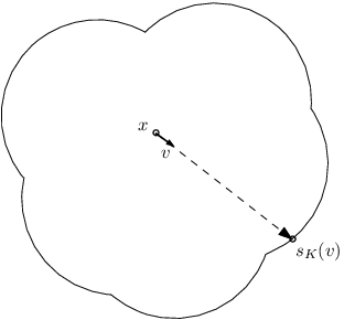
Lemma II.1.

Let $K=\{e\}\subseteq B(x,r)$ and define $s_{e}$ as above. Then $s_{e}$ is $2r$ -Lipschitz (with respect to the sphere’s inner metric) and its Jacobian is at most $(2r)^{n-1}$ .

Proof.

Solving the equation $\left\|x+tv-e\right\|=r$ with $t\geqslant 0$ gives

s_{e}(v)=x+\left(\sqrt{\langle v|x-e\rangle^{2}+r^{2}-\left\|x-e\right\|^{2}}-\langle v|x-e\rangle\right)v

Denote by $H_{v}$ the orthogonal of the $2$ -plane $P$ spanned by $v$ and $s_{e}(v)-e$ . For each vector $w$ chosen in $H_{v}$ , a simple calculation gives:

s_{e}(v+tw)=s_{e}(v)+tw\left\|s_{e}(v)-x\right\|+o(t^{2})

Hence the derivative of $s_{e}$ along $H_{v}$ is simply the multiplication by $\left\|s_{e}(v)-x\right\|\leqslant 2r$ .

Now, we now consider the case of the $2$ -plane $P$ . We denote by $\theta$ the angle between $s_{e}(v)-x$ and $s_{e}(v)-e$ and by $w$ a vector tangent to $v$ in the intersection of the sphere with $P$ . Then

\frac{\left\|(\mathrm{d}s_{e})_{v}(w)\right\|}{\left\|w\right\|}=\frac{\left\|s_{e}(v)-x\right\|}{\left|\cos(\theta)\right|}

Now let us remark that

	$\displaystyle\left\\|s_{e}(v)-e\right\\|\left\\|s_{e}(v)-x\right\\|\left\|\cos(\theta)\right\|$	$\displaystyle=\left\|\langle s_{e}(v)-e\|s_{e}(v)-x\rangle\right\|$
		$\displaystyle=\frac{1}{2}(\left\\|x-s_{e}(v)\right\\|^{2}+\left\\|s_{e}(v)-e\right\\|^{2}-\left\\|x-e\right\\|^{2})$
		$\displaystyle\geqslant\frac{1}{2}\left\\|x-s_{e}(v)\right\\|^{2}$

Finally we have proved that $\left\|(\mathrm{d}s_{e})_{v}\right\|\leqslant 2r$ . The result follows by integration. ∎

We denote by $\omega_{n}(r)$ the $n$ -Hausdorff measure of the $n$ -sphere of radius $r$ .

Corollary II.2.

A $r$ -flower in $\mathbb{R}^{n}$ is a $\mathcal{H}^{n-1}$ –rectifiable set and its measure is at most $\omega_{n-1}(2r)$ .

Proof.

Let $K\subseteq B(x,r)$ be the compact set generating the flower $\partial K^{r}$ . As above, for any vector $v\in\mathcal{S}^{n-1}$ , we denote by $s$ the intersection of the ray $\{x+tv\,;\,t>0\}$ with $\partial K^{r}$ . Since $K^{r}$ is a star-shaped set around $x$ , $s$ is a bijection from $\mathcal{S}^{n-1}$ to $\partial K^{r}$ .

Now let $(y_{k})$ be a dense sequence in $K$ , and denote by $s_{k}$ the projection from $\mathcal{S}^{n-1}$ to the flower $\partial(\cup_{i\leqslant k}\{y_{i}\})^{r}$ defined as above. Then $(s_{k})$ converges simply to $p$ on $\mathcal{S}^{n-1}$ . Indeed, if we fix $v\in\mathcal{S}^{n-1}$ and $\varepsilon>0$ , the segment joining $x$ and $s(v)$ truncated at a distance $\varepsilon$ of $s(v)$ is a compact set contained in $\interieur{K^{r}}$ . It is covered by the union $\cup_{i}B(y_{i},r)$ , so that for $N$ big enough it is also covered by $\cup_{k\leqslant N}B(y_{k},r)$ . For those $N$ , $\left\|s_{k}(x)-s(x)\right\|\leqslant\varepsilon$ .

Finally, $\partial K^{r}$ is the image of the sphere by $p$ , which is $2r$ -Lipschitz as a simple limit of $2r$ -Lipschitz functions. ∎

We now deduce a general bound on the measure of the tube boundary $\partial K^{r}$ around a general compact set $K$ by covering it with a family of flowers:

Theorem II.3.

If $K$ is a compact set of $\mathbb{R}^{n}$ , for every positive $r$ , $\partial K^{r}$ is a $\mathcal{H}^{n-1}$ -rectifiable subset of $\mathbb{R}^{n}$ and moreover,

\mathcal{H}^{n-1}(\partial K^{r})\leqslant\mathcal{N}(\partial K,r)\times\omega_{n-1}(2r)

Proof.

It is easy to see that $\partial K^{r}\subseteq\partial(\partial K^{r})$ . Thus, if we let $(x_{i})$ be an optimal covering of $\partial K$ by open balls of radius $r$ , and denote by $K_{i}$ the (compact) intersection of $\partial K$ with $B(x_{i},r)$ , the boundary $\partial K^{r}$ is contained in the union $\cup_{i}\partial K_{i}^{r}$ . Hence its Hausdorff measure does not exceed the sum $\sum_{i}\mathcal{H}^{n-1}(\partial K_{i}^{r})$ . One concludes by applying the preceding lemma.

∎

Remark II.4.

1.

The bound in the theorem is tight, as one can check taking $K=B(0,r)$ .

Let us notice that for some constant $C(n)$ , $\mathcal{N}(B(0,1),r)\leqslant 1+C(n)r^{-n}$ . From this and the above bound it follows that

	$\displaystyle\mathcal{H}^{n-1}(\partial K^{r})$	$\displaystyle\leqslant(1+C(n)\times(\diam(K)/r)^{n})\omega_{n-1}(2r)$
		$\displaystyle\leqslant C^{\prime}(n)\times(1+\frac{\diam(K)^{n}}{r})$

for some universal constant $C^{\prime}(n)$ depending only on the ambient dimension $n$ . This last inequality was the one proved in [OP85].

To conclude we use a weak formulation of the co-area formula, a standard result of geometric measure theory ([DG54], [Fed59]), which reads

\int_{\mathbb{R}^{n}}\left|\nabla_{x}f\right|\mathrm{d}\mathcal{H}^{n}(x)=\int_{\mathbb{R}}\mathcal{H}^{n-1}(f^{-1}(y))\mathrm{d}\mathcal{H}^{1}(y)

whenever $f:\mathbb{R}^{n}\to\mathbb{R}$ is a Lipschitz map. From this formula and the previous estimation follows that

Corollary II.5.

For any compact sets $K,K^{\prime}\subseteq\mathbb{R}^{n}$ , with $\mathrm{d}_{H}(K,K^{\prime})\leqslant\varepsilon$ ,

	$\displaystyle\mathcal{H}^{n}(K^{r}\Delta{K^{\prime}}^{r})$	$\displaystyle\leqslant\int_{r-\varepsilon}^{r+\varepsilon}\mathcal{H}^{n-1}(\partial K^{t})\mathrm{d}t$
		$\displaystyle\leqslant 2\mathcal{N}(K,r-\varepsilon)\omega_{n-1}(2r+2\varepsilon)\times\varepsilon$

III The map $K\mapsto p_{K}$ is locally $1/2$ -Hölder

We now study the continuity modulus of the map $K\mapsto p_{K}\in\mathrm{L}^{1}(E)$ , where $E$ is a suitable open set. We remind the reader of two well-known facts of convex analysis (see for instance [Cla83]):

1.

If $f:\Omega\subseteq\mathbb{R}^{n}\to\mathbb{R}$ is a locally convex function, its subdifferential at a point $x$ , denoted by $\partial_{x}f$ is the set of vectors $v$ of $\mathbb{R}^{n}$ such that for all $h\in\mathbb{R}^{n}$ small enough, $f(x+h)\geqslant f(x)+\langle h|v\rangle$ . Then $f$ admits a derivative at $x$ iff $\partial_{x}f=\{v\}$ is a singleton, in which case $\nabla_{x}f=v$ .
2.

A locally convex function has a derivative almost everywhere.

Lemma III.1.

The function $v_{K}:\mathbb{R}^{n}\to\mathbb{R},x\mapsto\left\|x\right\|^{2}-\mathrm{d}_{K}(x)^{2}$ is convex with gradient $\nabla v_{K}=2p_{K}$ almost everywhere.

Proof.

By definition, $v_{K}(x)=\sup_{y\in K}\left\|x\right\|^{2}-\left\|x-y\right\|^{2}=\sup_{y\in K}v_{K,y}(x)$ with $v_{K,y}(x)=2\langle x|y\rangle-\left\|y\right\|^{2}$ . Hence $v_{K}$ is convex as a supremum of affine functions. Because $v_{K,p_{K}(x)}$ and $v_{K}$ take the same value at $x$ , $\partial_{x}v_{K,p_{K}(x)}=\{2p_{K}(x)\}\subseteq\partial v_{K}$ . Since $v_{K}$ is differentiable almost everywhere, equality must be true almost everywhere which concludes the proof. ∎

This lemma shows that $\left\|p_{K}-p_{K^{\prime}}\right\|_{\mathrm{L}^{1}(E)}=1/2\left\|\nabla v_{K}-\nabla v_{K^{\prime}}\right\|_{\mathrm{L}^{1}(E)}$ . Our estimation of the continuity modulus of the map $K\mapsto\mathrm{p}_{K}$ will follow from a general theorem which asserts that if $\varphi$ and $\psi$ are two uniformly close convex functions with bounded gradients then $\nabla\varphi$ and $\nabla\psi$ are $\mathrm{L}^{1}$ -close. The next proposition below is the $1$ -dimensional version of this result, from which we then deduce the general theorem.

Proposition III.2.

If $I$ is an interval, and $\varphi:I\to\mathbb{R}$ and $\psi:I\to\mathbb{R}$ are two convex functions such that $\diam(\varphi^{\prime}(I)\cup\psi^{\prime}(I))\leqslant k$ , then letting $\delta=\left\|\varphi-\psi\right\|_{\mathrm{L}^{\infty}(I)}$ ,

\int_{I}\left|\varphi^{\prime}-\psi^{\prime}\right|\leqslant 6\pi(\mathrm{length}(I)+k+\delta^{1/2})\delta^{1/2}

Lemma III.3.

Let $f:I\to\mathbb{R}$ be a nondecreasing function with $\diam\varphi(I)\leqslant k$ . Then, if $F$ is the completed graph of $f$ , ie. the set of points $(x,y)\in I\times\mathbb{R}$ such that $\lim_{x^{-}}\varphi\leqslant y\leqslant\lim_{x^{+}}\varphi$ , then $\mathcal{H}^{n}(F^{r})\leqslant 3\pi(\mathrm{length}(I)+k+r)\times r$ .

Proof.

Let $\gamma:[0,1]\to F$ be a continuous parametrization of $F$ , increasing with respect to the lexicographic order on $\mathbb{R}^{2}$ . Then, for any increasing sequence $(t_{i})\in[0,1]$ and $(x_{i},y_{i})=\gamma(t_{i})$ ,

\sum_{i}\left\|\gamma(t_{i+1})-\gamma(t_{i})\right\|\leqslant\sum_{i}x_{i+1}-x_{i}+y_{i+1}-y_{i}\leqslant\mathrm{length}(I)+k

Hence $\mathrm{length}(F)\leqslant\mathrm{length}(I)+k$ . Thus we can choose a $1$ -Lipschitz parametrization of $F$ , $\tilde{\gamma}:[0,\mathrm{length}(I)+k]\to F$ . Then for any positive $r$ , the set $X=\{\tilde{\gamma}(i\times r)\,;\,0\leqslant i\leqslant N\}$ with $N$ the upper integer part of $(\mathrm{length}(I)+k)/r$ , is such that any point of $F$ is at distance at most $r$ of $X$ . Hence $F^{r}$ is contained in $X^{2r}$ , implying that $\mathcal{H}^{n}(F^{r})\leqslant N\pi(3r/2)^{2}\leqslant 3\pi(\mathrm{length}(I)+k+r)r$ . ∎

Proof of proposition III.2.

Let $I=[a,b]$ and $J=[c,c+k]$ be such that $\varphi^{\prime}(I)\cup\psi^{\prime}(I)\subseteq J$ . Without loss of generality we will suppose that $\psi^{\prime}(a)=\varphi^{\prime}(a)=c$ and $\psi^{\prime}(b)=\varphi^{\prime}(b)=c+k$ . With this assumption, the completed graphs $\Phi$ and $\Psi$ of $\varphi^{\prime}$ and $\psi^{\prime}$ defined as above are two rectifiable curves joining $(a,c)$ and $(b,c+k)$ . We let $V$ be the set of points $(x,y)\in\mathbb{R}^{2}$ lying between those graphs; the quantity we want to bound is $\int_{I}\left|\varphi^{\prime}-\psi^{\prime}\right|=\mathcal{H}^{2}(V)$ .

Let $\delta=\left\|\varphi-\psi\right\|_{\mathrm{L}^{\infty}(I)}$ . For any point $p=(x,y)$ in $V$ , and any $\delta^{\prime}>\delta$ , the closed disk $D=\overline{B}(p,\sqrt{2\delta^{\prime}/\pi})$ of volume $2\delta^{\prime}$ centered at $p$ cannot be contained in $V$ . Indeed if it were, then the difference $\kappa=\varphi-\psi$ would increase too much around $p$ : since $\kappa^{\prime}$ has a constant sign on this segment,

\left|\kappa(x+2\delta^{\prime}/\pi)-\kappa(x-2\delta^{\prime}/\pi)\right|=\int_{x-2\delta^{\prime}/\pi}^{x+2\delta^{\prime}/\pi}\left|\kappa^{\prime}\right|\geqslant\mathcal{H}^{2}(D)=2\delta^{\prime}>2\delta

This contradicts $\left\|\kappa\right\|_{\infty}=\delta$ . Hence, $D$ must intersects $\partial V$ implying that $V$ must be contained in $(\partial V)^{\sqrt{2\delta^{\prime}/\pi}}$ for any $\delta^{\prime}>\delta$ . Since $\partial V=\Phi\cup\Psi$ , the previous lemma gives

\mathcal{H}^{2}(V)\leqslant\mathcal{H}^{2}\left(\Phi^{\sqrt{2\delta^{\prime}/\pi}}\right)+\mathcal{H}^{2}\left(\Psi^{\sqrt{2\delta^{\prime}/\pi}}\right)\leqslant 6\pi(\mathrm{length}(I)+k+\sqrt{2\delta^{\prime}/\pi})\sqrt{2\delta^{\prime}/\pi}

Letting $\delta^{\prime}$ converge to $\delta$ concludes the proof. ∎

A generalization of this proposition in arbitrary dimension will follow from an argument coming from integral geometry, ie. we will integrate the inequality of proposition III.2 over the set of lines of $\mathbb{R}^{n}$ to get a bound on $\left\|\nabla\varphi-\nabla\psi\right\|_{\mathrm{L}^{1}(E)}$ .

We let $\mathcal{L}^{n}$ be the set of oriented affine lines in $\mathbb{R}^{n}$ seen as the submanifold of $\mathbb{R}^{2n}$ made of points $(u,p)\in\mathbb{R}^{n}\times\mathbb{R}^{n}$ with $u\in\mathcal{S}^{n-1}$ and $x$ in the hyperplane $\{u\}^{\bot}$ , and endowed with the induced Riemannian metric. The corresponding measure $\mathrm{d}\mathcal{L}^{n}$ is invariant under rigid motions. We let $\mathcal{D}_{u}^{n}$ be the set of oriented lines with a fixed direction $u$ .

The usual Crofton formula (cf. [Mor88] for instance) states that for any $\mathcal{H}^{n-1}$ –rectifiable subset $S$ of $\mathbb{R}^{n}$ , with $\beta_{n}$ the volume of the unit $n$ -ball,

\mathcal{H}^{n-1}(S)=\frac{1}{2\beta_{n-1}}\int_{\ell\in\mathcal{L}^{n}}\#(\ell\cap S)\mathrm{d}\ell

(III.1)

where $\#X$ is the cardinality of $X$ . We will also use the following Crofton-like formula: if $K$ is a $\mathcal{H}^{n}$ –rectifiable subset of $\mathbb{R}^{n}$ ,

\mathcal{H}^{n}(K)=\frac{1}{\omega_{n-1}}\int_{\ell\in\mathcal{L}^{n}}\mathcal{H}^{1}(\ell\cap K)\mathrm{d}\ell

(III.2)

which follows from the Fubini theorem (remember $\omega_{n-1}$ is the volume of the $(n-1)$ –sphere).

Lemma III.4.

Let $X:E\to\mathbb{R}^{n}$ be a $\mathrm{L}^{1}$ -vector field on an open subset $E\subseteq\mathbb{R}^{n}$ .

\int_{E}\left\|X\right\|=\frac{n}{2\omega_{n-2}}\int_{\ell\in\mathcal{L}^{n}}\int_{y\in\ell\cap E}\left|\langle X(y)|u(\ell)\rangle\right|\mathrm{d}y\mathrm{d}\ell

Sketch of proof.

The family of vector fields of the form $\sum_{i}X_{i}\chi_{\Omega_{i}}$ , where the $\Omega_{i}$ are a finite number of disjoint open subsets of $\mathbb{R}^{n}$ and $X_{i}$ are constant vectors, is $\mathrm{L}^{1}$ -dense in the space $\mathrm{L}^{1}(\mathbb{R}^{n},\mathbb{R}^{n})$ . Using this fact and the continuity of the two sides of the equality, it is enough to prove this equality for $X=x\left\|X\right\|\chi_{E}$ where $x$ is a constant unit vector and $E$ a bounded open set of $\mathbb{R}^{n}$ .

In that case, one has

	$\displaystyle\int_{\ell\in\mathcal{D}_{u}^{n}}\int_{y\in\ell}\left\|\langle X(y)\|u\rangle\right\|\mathrm{d}y\mathrm{d}\ell$	$\displaystyle=\left\\|X\right\\|\left\|\langle x\|u\rangle\right\|\int_{\ell\in\mathcal{D}_{u}^{n}}\mathrm{length}(E\cap\ell)\mathrm{d}\ell$
		$\displaystyle=\left\\|X\right\\|_{\mathrm{L}^{1}(E)}\left\|\langle x\|u\rangle\right\|$

By a Fubini-like theorem one has

	$\displaystyle\int_{\ell\in\mathcal{L}^{n}}\int_{y\in\ell}\left\|\langle X(y)\|u(\ell)\rangle\right\|\mathrm{d}y\mathrm{d}\ell$	$\displaystyle=\int_{u\in\mathcal{S}^{n-1}}\int_{\ell\in\mathcal{D}_{u}^{n}}\int_{y\in\ell}\left\|\langle X(y)\|u(\ell)\rangle\right\|\mathrm{d}y\mathrm{d}\ell\mathrm{d}u$
		$\displaystyle=\left\\|X\right\\|_{\mathrm{L}^{1}(E)}\int_{u\in\mathcal{S}^{n-1}}\left\|\langle x\|u\rangle\right\|\mathrm{d}u$

The last integral does, in fact, not depend on $x$ and its value can be easily computed:

	$\displaystyle\int_{u\in\mathcal{S}^{n-1}}\left\|\langle x\|u\rangle\right\|\mathrm{d}u$	$\displaystyle=2\omega_{n-2}\int_{0}^{1}t(1-t^{2})^{\frac{n}{2}-1}\mathrm{d}t$
		$\displaystyle=\frac{2}{n}\omega_{n-2}$

∎

Theorem III.5.

Let $E$ be an open subset of $\mathbb{R}^{n}$ with $(n-1)$ –rectifiable boundary, and $f,g$ be two locally convex functions on $E$ such that $\diam(\nabla f(E)\cup\nabla g(E))\leqslant k$ . Then, letting $\delta=\left\|f-g\right\|_{\mathrm{L}^{\infty}(E)}$

\left\|\nabla f-\nabla g\right\|_{\mathrm{L}^{1}(E)}\leqslant C_{1}(n)(\mathcal{H}^{n}(E)+(k+\delta^{1/2})\mathcal{H}^{n-1}(\partial E))\delta^{1/2}

with $C_{1}(n)\leqslant 6\pi n$ as soon as $n>5$ (in fact, $C_{1}(n)=O(\sqrt{n})$ ).

Proof of the theorem.

The $1$ -dimensional case follows from proposition III.2: in that case, $E$ is a countable union of intervals on which $f$ and $g$ satisfy exactly the hypothesis of the proposition. Summing the inequalities gives the result with $C_{1}(1)=6\pi$ .

The general case will follow from this one with the use of integral geometry. If we set $X=\nabla f-\nabla g$ , $f_{\ell}=\left.f\right|_{\ell\cap E}$ and $g_{\ell}=\left.g\right|_{\ell\cap E}$ . Lemma III.4 gives, letting $D(n)=n/(2\omega_{n-2})$ ,

	$\displaystyle\int_{E}\left\\|\nabla f-\nabla g\right\\|$	$\displaystyle=D(n)\int_{\ell\in\mathcal{L}^{n}}\int_{y\in\ell\cap E}\left\|\langle\nabla f-\nabla g\|u(\ell)\rangle\right\|\mathrm{d}y\mathrm{d}\ell$
		$\displaystyle=D(n)\int_{\ell\in\mathcal{L}^{n}}\int_{y\in\ell\cap E}\left\|f^{\prime}_{\ell}-g^{\prime}_{\ell}\right\|\mathrm{d}y\mathrm{d}\ell$

The functions $f_{\ell}$ and $g_{\ell}$ satisfy the hypothesis of the one-dimensional case, so that for each choice of $\ell$ , and with $\delta=\left\|f-g\right\|_{\mathrm{L}^{\infty}(E)}$ ,

\int_{y\in\ell\cap E}\left|f^{\prime}_{\ell}-g^{\prime}_{\ell}\right|\mathrm{d}y\leqslant 6\pi D(n)(\mathcal{H}^{1}(E\cap\ell)+(k+\delta^{1/2})\mathcal{H}^{0}(\partial E\cap\ell))\delta^{1/2}

It follows by integration on $\mathcal{L}^{n}$ that

\int_{E}\left\|\nabla f-\nabla g\right\|\leqslant 6\pi D(n)\left(\int_{\mathcal{L}^{n}}\mathcal{H}^{1}(E\cap\ell)\mathrm{d}\mathcal{L}^{n}+(k+\delta^{1/2})\int_{\mathcal{L}^{n}}\mathcal{H}^{0}(\partial E\cap\ell)\mathrm{d}\mathcal{L}^{n}\right)\delta^{1/2}

The formula III.1 and III.2 show that the first integral is equal (up to a constant) to the volume of $E$ and the second to the $(n-1)$ -measure of $\partial E$ . This proves the theorem with $C_{1}(n)=6\pi D(n)(\omega_{n-1}+2\beta_{n-1})$ . To get the bound on $C_{1}(n)$ one uses the formula $\omega_{n-1}=n\beta_{n}$ and $\beta_{n+1}\leqslant\beta_{n}$ as soon as $n>5$ . ∎

Multiplying $f$ and $g$ by the same positive factor $t$ and optimizing the result in $t$ yields a better, homogeneous, bound :

Corollary III.6.

Under the same hypothesis as in theorem III.5, one gets the following bound, with $\delta=\left\|f-g\right\|_{\mathrm{L}^{\infty}(E)}$ :

	$\displaystyle\left\\|\nabla f-\nabla g\right\\|_{\mathrm{L}^{1}(E)}\leqslant 2C_{1}(n)[(\mathcal{H}^{n}(E)\mathcal{H}^{n-1}(\partial E)$	$\displaystyle\diam(\nabla f(E)\cup\nabla g(E)))^{1/2}$
		$\displaystyle+\mathcal{H}^{n-1}(\partial E)\delta^{1/2}]\delta^{1/2}$

Remark III.7.

To get an homogeneous bound as in this corollary, one could also optimize the one-dimensional bound of proposition III.2 before integrating on the set of affine lines of $\mathbb{R}^{n}$ as in the proof of theorem III.5. The bound obtained this way is always strictly better than the ones of both theorem III.5 and corollary III.6, but involves an integral term

\int_{\ell\in\mathcal{L}^{n}}\sqrt{\mathcal{H}^{0}(\ell\cap\partial E)\mathcal{H}^{1}(\ell\cap E)}\mathrm{d}\ell

whose intuitive meaning is not quite clear.

Applying theorem III.5 to the functions $v_{K}$ and $v_{K^{\prime}}$ introduced at the begining of this part and using lemma III.1, one easily gets :

Corollary III.8.

If $E$ is an open set of $\mathbb{R}^{n}$ with rectifiable boundary, $K$ and $K^{\prime}$ two compact subsets of $\mathbb{R}^{n}$ then, with $R_{K}=\left\|d_{K}\right\|_{\mathrm{L}^{\infty}(E)}$ and $\varepsilon=\mathrm{d}_{H}(K,K^{\prime})$ ,

	$\displaystyle\left\\|p_{K}-p_{K^{\prime}}\right\\|_{\mathrm{L}^{1}(E)}\leqslant C_{1}(n)[\mathcal{H}^{n}(E)+(\diam$	$\displaystyle(K)+\varepsilon+(2R_{K}+\varepsilon)^{1/2}\varepsilon^{1/2})\mathcal{H}^{n-1}(\partial E)]$
		$\displaystyle\times(2R_{K}+\varepsilon)^{1/2}\varepsilon^{1/2}$

In particular, if $\mathrm{d}_{H}(K,K^{\prime})$ is smaller than $\min(R_{K},\diam(K),\diam(K)^{2}/R_{K})$ , there is another constant $C_{2}(n)$ depending only on $n$ such that

\left\|p_{K}-p_{K^{\prime}}\right\|_{\mathrm{L}^{1}(E)}\leqslant C_{2}(n)[\mathcal{H}^{n}(E)+\diam(K)\mathcal{H}^{n-1}(\partial E)]\sqrt{R_{K}\mathrm{d}_{H}(K,K^{\prime})}

Remarks III.9.

1.

This theorem gives in particular a quantitative version of the continuity theorem $4.13$ of [Fed59]: if $(K_{n})$ is a sequence of compact subsets of $\mathbb{R}^{n}$ with $\reach(K_{n})\geqslant r>0$ , converging to a compact set $K$ , then $\reach(K)\geqslant r$ and $\mathrm{p}_{K_{n}}$ converges to $\mathrm{p}_{K}$ uniformly on each compact set contained in $\{x\in\mathbb{R}^{n}\,;\,\mathrm{d}_{K}(x)<r\}$ . However we have to stress that the result we have proved is more general since it does not make any assumption on the regularity of $K_{n}$ — at the expense of uniform convergence.
2.

The second term of the bound involving $\mathcal{H}^{n-1}(\partial E)$ is necessary. Indeed, let us suppose that a bound $\left\|p_{K}-p_{K^{\prime}}\right\|_{\mathrm{L}^{1}(E)}\leqslant C(K)\mathcal{H}^{n}(E)\sqrt{\varepsilon}$ were true around $K$ for any open set $E$ . Now let $K$ be the union of two parallel hyperplane at distance $R$ intersected with a big sphere centered at a point $x$ of their medial hyperplane $M$ . Let $E_{\varepsilon}$ be a ball of radius $\varepsilon$ tangent to $M$ at $x$ and $K_{\varepsilon}$ be the translation by $\varepsilon$ of $K$ along the common normal of the hyperplanes such that the medial hyperplane of $K_{\varepsilon}$ touches the ball $E_{\varepsilon}$ on the opposite of $x$ . Then, for $\varepsilon$ small enough, $\left\|p_{K}-p_{K^{\prime}}\right\|_{\mathrm{L}^{1}(E_{\varepsilon})}\simeq R\times\mathcal{H}^{n}(E_{\varepsilon})$ , which clearly exceeds the assumed bound for a small enough $\varepsilon$ .
3.

According to this theorem, the map $K\mapsto p_{K}\in\mathrm{L}^{1}(E)$ is locally $1/2$ -Hölder. The following example shows that this result cannot be improved even around a very simple compact set.

Figure III.3: A sequence of «knife blades» converging to a segment.

Let $S$ and $S^{\prime}$ be two opposite sides of a rectangle $E$ , ie. two segments of length $L$ and at distance $R$ . We now define a Hausdorff approximation of $S$ : for any positive integer $N$ , divide $S$ in $N$ small segments $s^{i}$ of common length $\ell$ , and let $C_{i}$ be the unique circle with center in $S^{\prime}$ which contains the two endpoints of $s^{i}$ . We now let $S_{N}$ be the union of the circle arcs of $C_{i}$ comprised between the two endpoints of $s^{i}$ .

Then it is not very hard to see that if $R_{\varepsilon}=R+\varepsilon$ is the common radius of all the $C^{i}$ , $R_{\varepsilon}^{2}=R^{2}+(\ell/2)^{2}$ , ie. $\mathrm{d}_{H}(S,S_{N})=\sqrt{R^{2}+(\ell/2)^{2}}-R\leqslant R\ell^{2}/8$ . Then the $\mathrm{L}^{1}$ -distance between the projections on $S$ and $S_{N}$ is at least $\Omega(\ell)$ (because almost half of the points in $E$ projects on the corners of $S_{N}$ , see the shaded area in fig. III.3). Hence,

$\left\|p_{S}-p_{S_{N}}\right\|_{\mathrm{L}^{1}(E)}=\Omega(\ell)=\Omega(\mathrm{d}_{H}(S,S_{N})^{1/2})$

Replacing $\mathrm{L}^{1}(E)$ with $\mathrm{L}^{1}(\mu)$ where $\mu$ has bounded variation

As we have seen before, a corollary of the previous result is that if $\mu=\left.\mathcal{H}^{n}\right|_{E}$ , the map $K\mapsto\mathrm{p}_{K\#}\mu$ is locally $1/2$ -Hölder. This result can be generalized when $\mu=u\mathcal{H}^{n}$ where $u\in\mathrm{L}^{1}_{\mathrm{loc}}(\mathbb{R}^{n})$ has bounded variation. We recall some facts about the theory of functions with bounded variation, taken from [AFP00]. If $\Omega\subseteq\mathbb{R}^{n}$ is an open set and $u\in\mathrm{L}^{1}_{\mathrm{loc}}(\Omega)$ , the variation of $u$ in $\Omega$ is

\var(u,\Omega)=\sup\left\{\int_{\Omega}u\ddiv\varphi;\varphi\in\mathcal{C}^{1}_{c}(\Omega),\left\|\varphi\right\|_{\infty}\leqslant 1\right\}

A function $u\in\mathrm{L}^{1}_{\mathrm{loc}}(\Omega)$ has bounded variation if $V(u,\Omega)<+\infty$ . The set of functions of bounded variation on $\Omega$ is denoted by $\BV(\Omega)$ . We also mention that if $u$ is Lipschitz on $\Omega$ , then $\var(u,\Omega)=\left\|\nabla u\right\|_{\mathrm{L}^{1}(\Omega)}$ . Finally, we let $\var(u)$ be the total variation of $u$ in $\mathbb{R}^{n}$ .

Theorem III.10.

Let $\mu\in\mathcal{M}(\mathbb{R}^{n})$ be a measure with density $u\in\BV(\mathbb{R}^{n})$ with respect to the Lebesgue measure, and $K$ be a compact subset of $\mathbb{R}^{n}$ . We suppose that $\supp(u)\subseteq K^{R}$ . Then, if $\mathrm{d}_{H}(K,K^{\prime})$ is small enough,

d_{\mathrm{bL}}(\mathrm{p}_{K\#}\mu,\mathrm{p}_{K^{\prime}\#}\mu)\leqslant C_{2}(n)\left(\left\|u\right\|_{\mathrm{L}^{1}(K^{R})}+\diam(K)\var\left(u\right)\right)\sqrt{R}\times\mathrm{d}_{H}(K,K^{\prime})^{1/2}

Proof.

We begin with the additional assumption that $u$ has class $\mathcal{C}^{\infty}$ . The function $u$ can be written as an integral over $t\in\mathbb{R}$ of the characteristic functions of its superlevel sets $E_{t}=\{u>t\}$ , ie. $u(x)=\int_{0}^{\infty}\chi_{E_{t}}(x)\mathrm{d}t$ . Fubini’s theorem then ensures that for any Lipschitz function $f$ defined on $\mathbb{R}^{n}$ with $\left\|f\right\|_{\mathrm{Lip}}\leqslant 1$ ,

	$\displaystyle\mathrm{p}_{K^{\prime}\#}\mu(f)$	$\displaystyle=\int_{\mathbb{R}^{n}}f\circ\mathrm{p}_{K^{\prime}}(x)u(x)\mathrm{d}x$
		$\displaystyle=\int_{\mathbb{R}}\int_{\mathbb{R}^{n}}f\circ\mathrm{p}_{K^{\prime}}(x)\chi_{\{u\geqslant t\}}(x)\mathrm{d}x\mathrm{d}t$

By Sard’s theorem, for almost any $t$ , $\partial E_{t}=u^{-1}(t)$ is a $(n-1)$ -rectifiable subset of $\mathbb{R}^{n}$ . Thus, for those $t$ the previous corollary implies, for $\varepsilon=\mathrm{d}_{H}(K,K^{\prime})\leqslant\varepsilon_{0}=\min(R,\diam(K),\diam(K)^{2}/R_{K})$ ,

	$\displaystyle\int_{E_{t}}\left\|f\circ\mathrm{p}_{K}(x)-f\circ\mathrm{p}_{K^{\prime}}(x)\right\|\mathrm{d}x$	$\displaystyle\leqslant\left\\|\mathrm{p}_{K}-\mathrm{p}_{K^{\prime}}\right\\|_{\mathrm{L}^{1}(E_{t})}$
		$\displaystyle\leqslant C_{2}(n)[\mathcal{H}^{n}(E_{t})+\diam(K)\mathcal{H}^{n-1}(\partial E_{t})]\sqrt{R\varepsilon}$

Putting this inequality into the last equality gives

\left|p_{K\#}\mu(f)-p_{K^{\prime}\#}\mu(f)\right|\leqslant C_{2}(n)\left(\int_{\mathbb{R}}\mathcal{H}^{n}(E_{t})+\diam(K)\mathcal{H}^{n-1}(\partial E_{t})\mathrm{d}t\right)\sqrt{R\varepsilon}

Using Fubini’s theorem again and the coarea formula one finally gets that

\left|p_{K\#}\mu(f)-p_{K^{\prime}\#}\mu(f)\right|\leqslant C_{2}(n)\left(\left\|u\right\|_{\mathrm{L}^{1}(K^{R})}+\diam(K)\var(u)\right)\sqrt{R\varepsilon}.

This proves the theorem in the case of Lipschitz functions. To conclude the proof in the general case, one has to approximate the bounded variation function $u$ by a sequence of $\mathcal{C}^{\infty}$ functions $(u_{n})$ such that both $\left\|u-u_{n}\right\|_{\mathrm{L}^{1}(K^{R})}$ and $\left|\var(u)-\var(u_{n})\right|$ converge to zero, which is possible by theorem 3.9 in [AFP00]. ∎

Remark III.11.

Taking $u=\chi_{E}$ where $E$ is a suitable open set shows that theorem III.8 can also be recovered from III.10.

IV Stability of boundary and curvature measures

We combine the results of corollaries I.6, II.5 and III.8 to get

Theorem IV.1.

If $K$ and $K^{\prime}$ are two compact sets with $\varepsilon=\mathrm{d}_{H}(K,K^{\prime})$ smaller than $\min(\diam K,r,r^{2}/\diam K)$ , then

d_{\mathrm{bL}}(\mu_{K,r},\mu_{K^{\prime},r})\leqslant C_{3}(n)\mathcal{N}(K,r-\varepsilon)r^{n}[r+\diam(K)]\sqrt{\frac{\varepsilon}{r}}

In particular, if for a given bounded Lipschitz function $f$ on $\mathbb{R}^{n}$ , one defines $\varphi_{K,f}(r)=\mu_{K,r}(f)$ , the map $K\mapsto\varphi_{K,f}\in\mathcal{C}^{0}([r_{\mathrm{min}},r_{\mathrm{max}}])$ with $0<r_{\mathrm{min}}<r_{\mathrm{max}}$ is locally $1/2$ -Hölder.

In what follows we suppose that $(r_{i})$ is a sequence of $n$ distinct numbers $0<r_{0}<...<r_{n}$ . For any compact set $K$ and $f\in\mathcal{C}^{0}(\mathbb{R}^{n})$ , we let $\left[\Phi^{(r)}_{K,i}(f)\right]_{i}$ be the solutions of the linear system

\forall i\hbox{ s.t }0\leqslant i\leqslant n,~\sum_{j=0}^{n}\omega_{n-j}\Phi^{(r)}_{K,j}(f)r_{i}^{n-j}=\mu_{K,r_{i}}(f)

Since the system is linear in $(\mu_{K,r_{i}}(f))$ and these values depends continuously on $f$ , the map $f\mapsto\Phi_{K,i}^{(r)}(f)$ is also linear and continuous, ie. $\Phi^{(r)}_{K,i}$ is a signed measure on $\mathbb{R}^{n}$ . It is also to be noticed that if $K$ has positive reach with $\reach(K)>r_{n}$ , the $\Phi^{(r)}_{K,i}$ coincide with the usual curvature measures of $K$ . In that case, the following result gives a way to approximate the (usual) curvature measures of $K$ from a Hausdorff-approximation of it even if its reach is arbitrary small.

Corollary IV.2.

There exist a constant $C$ depending on $K$ and $(r)$ such that for any compact subset $K^{\prime}$ of $\mathbb{R}^{n}$ close enough to $K$ ,

\forall i,~d_{\mathrm{bL}}\left(\Phi_{K^{\prime},i}^{(r)},\Phi_{K,i}^{(r)}\right)\leqslant C\mathrm{d}_{H}(K,K^{\prime})^{1/2}

References

[AFP00] L. Ambrosio, N. Fusco, and D. Pallara. Functions of bounded variation and free discontinuity problems. Oxford Mathematical Monographs, 2000.
[BGV07] F. Bolley, A. Guillin, and C. Villani. Quantitative Concentration Inequalities for Empirical Measures on Non-compact Spaces. Probability Theory and Related Fields, 137(3):541–593, 2007.
[BKL06] A. Beygelzimer, S. Kakade, and J. Langford. Cover trees for nearest neighbor. Proceedings of the 23rd international conference on Machine learning, pages 97–104, 2006.
[BSK] G.H. Bendels, R. Schnabel, and R. Klein. Detecting Holes in Point Set Surfaces.
[Cla83] F.H. Clarke. Optimization and nonsmooth analysis. Wiley New York, 1983.
[DG54] E. De Giorgi. Su una teoria generale della misura (r- 1)-dimensionale in uno spazio adr dimensioni. Annali di Matematica Pura ed Applicata, 36(1):191–213, 1954.
[DGGZ03] T.K. Dey, J. Giesen, S. Goswami, and W. Zhao. Shape Dimension and Approximation from Samples. Discrete and Computational Geometry, 29(3):419–434, 2003.
[DHOS07] J. Daniels, L. K. Ha, T. Ochotta, and C. T. Silva. Robust smooth feature extraction from point clouds. In Shape Modeling International, 2007. Proceedings, 2007.
[Fed59] H. Federer. Curvature Measures. Transactions of the American Mathematical Society, 93(3):418–491, 1959.
[FK06] S. Funke and C. Klein. Hole detection or: how much geometry hides in connectivity? Proceedings of the twenty-second annual symposium on Computational geometry, pages 377–385, 2006.
[GWM01] S. Gumhold, X. Wang, and R. MacLeod. Feature extraction from point clouds. Proc. 10th International Meshing Roundtable, pages 293–305, 2001.
[Mor88] F. Morgan. Geometric Measure Theory: A Beginner’s Guide. Academic Press, 1988.
[OP85] I.Y. Oleksiv and NI Pesin. Finiteness of Hausdorff measure of level sets of bounded subsets of Euclidean space. Mathematical Notes, 37(3):237–242, 1985.
[RBBK06] G. Rosman, A. M. Bronstein, M. M. Bronstein, and R. Kimmel. Topologically constrained isometric embedding. In Proc. Conf. on Machine Learning and Pattern Recognition (MLPR), 2006.
[Vil03] C. Villani. Topics in Optimal Transportation. American Mathematical Society, 2003.
[Wey39] H. Weyl. On the Volume of Tubes. American Journal of Mathematics, 61(2):461–472, 1939.

	$\displaystyle\left\\|s_{e}(v)-e\right\\|\left\\|s_{e}(v)-x\right\\|\left\|\cos(\theta)\right\|$	$\displaystyle=\left\|\langle s_{e}(v)-e\|s_{e}(v)-x\rangle\right\|$
		$\displaystyle=\frac{1}{2}(\left\\|x-s_{e}(v)\right\\|^{2}+\left\\|s_{e}(v)-e\right\\|^{2}-\left\\|x-e\right\\|^{2})$
		$\displaystyle\geqslant\frac{1}{2}\left\\|x-s_{e}(v)\right\\|^{2}$

Introduction

Theorem (IV.1).

Theorem (III.5).

Theorem (II.3).

I Definition of boundary measures

Some examples of boundary measures

Notations.

Definition I.1.

Examples.

The boundary measure of a point cloud

Theorem I.2 (Hoeffding’s inequality).

Proposition I.3.

Proof.

Wasserstein distance and stability

Definition I.4.

Notations.

Proposition I.5.

Proof.

Corollary I.6.

II Kr​Δ​K′rK^{r}\Delta{K^{\prime}}^{r} is small when KK and K′K^{\prime} are close

Theorem.

Lemma II.1.

Proof.

Corollary II.2.

Proof.

Theorem II.3.

Proof.

Remark II.4.

Corollary II.5.

III The map K↦pKK\mapsto p_{K} is locally 1/21/2-Hölder

Lemma III.1.

Proof.

Proposition III.2.

Lemma III.3.

Proof.

Proof of proposition III.2.

Lemma III.4.

Sketch of proof.

Theorem III.5.

Proof of the theorem.

Corollary III.6.

Remark III.7.

Corollary III.8.

Remarks III.9.

Replacing L1​(E)\mathrm{L}^{1}(E) with L1​(μ)\mathrm{L}^{1}(\mu) where μ\mu has bounded variation

Theorem III.10.

Proof.

Remark III.11.

IV Stability of boundary and curvature measures

Theorem IV.1.

Corollary IV.2.

References

II $K^{r}\Delta{K^{\prime}}^{r}$ is small when $K$ and $K^{\prime}$ are close

III The map $K\mapsto p_{K}$ is locally $1/2$ -Hölder

Replacing $\mathrm{L}^{1}(E)$ with $\mathrm{L}^{1}(\mu)$ where $\mu$ has bounded variation