Arthur Jaffe and David Moser
Note: The authors thank an anonymous donor, whose
gift enabled this collaboration.
Affiliation: Harvard University
Affiliation: Cambridge, MA 02138, USA
Affiliation: Arthur_Jaffe@harvard.edu,
David.Moser@gmx.net
August 11, 2026
Abstract
We give an intuitive method—using local, cyclic replica symmetry—to isolate
exponential tree decay in truncated (connected) correlations. We give an
expansion and use the symmetry to show that all terms vanish, except those
displaying replica condensation. The condensation property ensures
exponential tree decay.
We illustrate our method in a low-temperature Ising system, but expect that one
can use a similar method in other random field and quantum field problems.
While considering the illustration, we prove an elementary upper bound on the
entropy of random lattice surfaces.
I Introduction
Symmetry is used widely in physics to unify laws or simplify results. Global
symmetries often arise and are characterized by Lie groups or their
representation acting on a manifold. Some symmetries, such as gauge symmetry,
are local; they are characterized by the action of a group on a bundle over a
manifold. Global replica symmetry has been introduced as a symmetry of the
Hamiltonian of certain interacting systems such as Ising models, random fields,
and quantum fields, leading to valuable insights.
In §III we study local replica symmetry. This is not a symmetry of the Hamiltonian in general, but it is a symmetry
within certain spin configurations. This enables us to simplify our expansion
of certain expectations in the low-temperature Ising system in order to exhibit
a desired property: exponential tree decay of truncated correlations. This
low-temperature expansion only serves to illustrate our method. We plan to
investigate the use of our method in other high-temperature and low-temperature
situations for random and quantum fields.
Consider the truncated expectations
, defined in §IV.1. The Ising spins are maps from the
unit lattice in dimensions to . The Hamiltonian is
, and the Gibbs factor is ,
where denotes the inverse temperature. We show in §VIII that there are constants such that for ,
(I.1)
where is the length of the minimal tree connecting the
points . Note the condition requires that
, where grows at least as fast as . It
would be of interest to eliminate the -dependence from the minimum value of
.
Our method uses replica variables, comprising identical, independent copies
of the original system; one considers expectations in the replicated system
that are product expectations for the individual systems. Replica symmetry is
the symmetry of these expectations under a permutation of the copies. For a
system in a finite volume , with , the same
estimate holds uniformly in . Our method requires unbroken replica
symmetry, so one must impose the same boundary conditions in each replica copy.
We develop a low-temperature expansion, based on the intuitive idea that
individual terms with less than the desired exponential tree-graph decay sum to
zero (vanish) due to symmetry under the local cyclic replica group. In §VIII we define and establish convergence of this expansion. The
terms in the expansion are parameterized by replica continents. These
replica continents are bounded by random surfaces. The convergence of our
expansion relies on an interplay between energy and entropy estimates; in
particular we give entropy estimates bounding the number of random surfaces
that occur in our expansion, as well as energy estimates showing that large
islands are suppressed at a desired rate.
Key to our method is the use of local cyclic replica symmetry, to show that all
non-zero terms in our expansion display replica condensation, defined in
§V. By this we mean that all the lattice sites
must live on a single continent. The size of the boundary of
the continent must therefore be larger than ; this is the
source of the exponential tree decay.
I.1 The Ising Model as Illustration
The Ising system is the simplest example of a
statistical mechanics interaction. We present our method for such a model on a
unit cubic lattice , with , although our methods clearly apply in
more generality. The Ising Hamiltonian in volume is
(I.2)
where denotes the sum over nearest-neighbor pairs of sites in the lattice,
namely sites with . The partition function
(I.3)
normalizes statistical averages of a function ,
namely
(I.4)
Often is a monomial in spins,
. The expectation is linear, so one can express the expectation of a general as a limit
of finite linear combinations of expectations of the form
.
II The Correspondence
Each subset of sites in the
lattice can be identified with a subset . Define the
latter as the union of closed, unit -cubes centered at the
lattice sites , as we illustrate in the upper part of Figure
1.
Figure 1: An example for the correspondence between subsets of and
, and their boundaries.
Connectedness:
We say that is connected if any two sites in can be
connected by a continuous path through nearest-neighbor lattice sites in the
set . This agrees with the notion that the interior of the set
is connected in the ordinary sense. Two cubes are connected if
they share a -dimensional face, but they are disconnected if they only
touch on a corner of dimension .
Boundary:
The boundary allows us to define the set of boundary lattice sites. These boundary sites are those lattice sites in lying in cubes that share a
-dimensional face with the boundary .
By we always refer to the area of the -dimensional
surface in and not the number of points in . (A single cube
, for example, contains exactly boundary lattice site, while
.) In most instances we will call this area the
“length” of the boundary, but in some cases we will also call it the number
of faces of the boundary surface. We illustrate the correspondence between the
boundary lattice sites and the boundary of regions in in the lower part
of Figure 1.
Surface:
More generally let a face in denote a
-cube; such a cube lies in the boundary of two -cubes in . A
surface is a union of -faces, and its area is the
number of -faces in . Lattice sites in may lie on either side of
the surface , but could be limited by selecting an orientation to
appropriate sets of faces in .
Connected Surface:
Define two faces to be adjacent, if they share a -cube.
Likewise, define to be connected if any two faces in can be
reached by a continuous path through a sequence of adjacent faces in .
III Replica Variables and Symmetry
Choose and consider independent copies of a
statistical-mechanical or quantum-field system; these are called replicas.
One can study the properties
of expectations under the group of permutations of the replica variables (the
replica group). The -element subgroup of cyclic permutation of all
the copies is abelian, and it provides useful one-dimensional representations
of replica symmetry.
III.1 Replica Variables
We assume that the different replicas are identical and independent. They are
defined on the same lattice, they have the same form of interaction, they are
given identical boundary conditions, etc. We label the spin variable at the
lattice site by , where
denotes the index of the copy. We also consider the replica spins at site
as a vector with the vector components .
III.2 The Global Replica Group
The global replica group is the symmetric group
comprising elements with action,
(III.1)
The element acts on the spins, giving a unitary
representation,
(III.2)
The global cyclic replica group is the subgroup of cyclic
permutations of objects, and is generated by the permutation ,
(III.3)
Treating the indices modulo , substitute for
and write
Let denote a subset of the lattice . The local cyclic
replica group is a bundle over defined as the action
of on the spins in and the identity on the complement. This
group is generated by which has the representation on spins,
(III.6)
III.4 Irreducible Representations
The cyclic replica group is abelian, so its irreducible representations are one
dimensional. We transform from to a set of coordinates to reduce the representation of . In particular, let
denote the primitive root of unity. Define
(III.7)
Note that for the -variables may be complex, even though the original
-spins are real. The choice (III.7) defines the entries of
the matrix as .
This is Fourier transform in the replica space.
Proposition III.1.
The matrix is unitary with eigenvalues , for
. Let be the diagonal matrix with . Then
(III.8)
Proof.
For an integer (modulo ),
(III.9)
Thus
(III.10)
Since acts on the components according to
(III.4), this means that
A further corollary of the unitarity of is the fact that for any
(III.13)
In particular, the expression on the right side of this identity is always
real. Furthermore, each individual term on the right is invariant under the
elements of the local, cyclic replica group as long as both
or both .
III.5 Replica Boundary Conditions
We consider finite volume Hamiltonians that, along with their boundary
conditions, have the global replica group as a symmetry. If one wished to
investigate the breaking of the replica group in the infinite volume limit,
then one might explicitly break replica symmetry in a finite volume by imposing
different boundary conditions for different replica copies of the system.
Since our system is originally given in terms of the variables , one
describes the boundary conditions in the volume in terms of the
variables for , with
defined in §II.
It is natural to ensure symmetry under the replica group by specifying the same
boundary condition on each component of the vector spin
(III.14)
In order to simplify the discussion, we impose boundary conditions in each
replica copy: set
(III.15)
The resulting boundary conditons for are
(III.16)
III.6 Replica Symmetry is Global, not Local
Define the total replica Hamiltonian as the sum of the
Hamiltonians for the replica copies of the Hamiltonian in volume ,
The replica Hamiltonian
(III.18) is invariant under a global replica permutation
defined in (III.2), namely
(III.19)
iii.
In general, the replica Hamiltonian is not invariant under the local
cyclic replica group defined in
(III.6).
Proof.
The relation (III.13) shows that has the form
(III.18). The invariance under the global replica
group follows by considering the effect on expressed in the
variables, where the transformation permutes the various terms
in the first expression for in
(III.17).
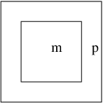
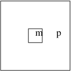
In order to see that is not invariant under the
local cyclic replica group, we give a configuration and set
that provides a counterexample in the case . It is easiest to
visualize this configuration by illustrating it; see the left side of Figure
2. We choose to be the centermost square
in the configuration (with and ), and choose
to flip the spins in . The action of
produces the configuration on the right side of the figure,
and it lowers the energy by . In other words, , showing that is not invariant
under the action of .
Figure 2: A counter-example to local cyclic replica symmetry.
∎
IV Expectations
Define the expectation for the
replicated system as follows: for a function , let
(IV.1)
where , with is given in (I.3).
In case that only depends on one
component , the expectation reduces to
the expectation . In this case
(IV.2)
We now introduce the generating function for expectations of products
of spins. Let be a function from to and let
(IV.3)
Then define
(IV.4)
The expectations of spins are derivatives of the generating function,
(IV.5)
The expectations (IV.5) are -multi-linear, symmetric,
functions of the spins,
(IV.6)
One can recover the expectation
from the expectations
of powers of by polarization,
(IV.7)
IV.1 Truncated Expectations
The truncated
expectation of a product of spins is a generalization of the correlation of
two spins. The truncated expectation vanishes asymptotically as one translates
any subset of the spin locations a large distance away from the others.
The generating function of the connected expectations is
(IV.8)
One defines the truncated (connected) expectations as
(IV.9)
A standard representation of
in terms of sums of products of expectations
can be formulated in terms of the set of partitions of
. Suppose that a set has cardinality
. Then
(IV.10)
Like the expectations (IV.5), the -truncated expectations
satisfy the -multi-linear relation
(IV.6)–(IV.7). Thus
(IV.11)
and
(IV.12)
IV.2 Truncated Functions as Replica Expectations
The form of the replica variables leads to an elementary
representation of the truncated (connected) expectations of products of spins.
Ultimately we show that this yields exponential decay at low temperatures with
a rate governed by the length of the shorted tree-graph connecting all the
spins. (A similar argument presumably works at high temperature.)
Our expansion method uses replica symmetry to arrange that each term in the
expansion either exhibits the desired decay rate, or else it is canceled by
other terms as a consequence of local cyclic replica symmetry. We begin by
establishing a known representation of the connected correlation of spins
as an expectation of replica variables introduced above. This
representation was discovered by P. Cartier (unpublished); our presentation is
based on Sylvester’s treatment [2] using . Let
denote the greatest common divisor.
Proposition IV.1.
Let be defined in (III.7)
with replica copies, and let satisfy
. Then
(IV.13)
Lemma IV.2.
For all ,
(IV.14)
Proof.
Using the multi-linearity (IV.11), and its analog for
the expectations and of the
truncated functions, we infer that
Since the different components of are independent, the
expectations on the right vanishes unless . In this
case the truncated expectation of each copy equals the truncated expectation of
the original spins, and the sum yields such terms. Therefore
(IV.14) holds as claimed.
∎
Lemma IV.3.
Let (modulo). Then
(IV.16)
Proof.
Expand the expectation
In the second equality, we use the symmetry of the expectation under the global cyclic replica group . Therefore
(IV.18)
As long as (modulo ), it is the case that . Therefore the expectation must vanish.
∎
Proof of the Proposition.
The relation
(IV.10) also holds for the replica expectations,
(IV.19)
Because , it is the case that (modulo ) for
all . Thus we can apply Lemma IV.3 to each such ,
and only the partition with all elements in one set survives in
(IV.19). We infer
In this section we investigate certain classes of configurations
of the replica spins. We see that for each class of configurations, there is a
local cyclic replica group (see §III.3) under which
the Hamiltonian of (III.17) is
invariant. This leads to the phenomenon of replica condensation in which
all the spin localizations must be localized within a given
region that we call a continent.
V.1 Continents
Each configuration of spins in the volume defines a
sea , surrounding a set of continents
. The sea starts at the boundary boundary of the region . The boundary of a continent appears if any
one of the components of changes its value. Continents have a
substructure arising from the different configurations of the individual
components within the continent. We say more about this
substructure when defining replica continent contours in
§VI.2. In the following we utilize the notion
of “connectedness” introduced in §II.
Definition V.1.
Consider a configuration . The replica sea
is the connected component of the set that meets the boundary of
. The continents are the connected components of the
complementary set,
The set of continents is
In §III.6 we saw that a global replica symmetry
transformation leaves invariant, and that a
local replica symmetry transformation does not necessarily do so. We now
recover local cyclic replica symmetry by choosing the localization in
to be a continent.
Proposition V.2.
Let . Then the local cyclic replica group defined in (III.6) preserves
the continent and the Hamiltonian . For
,
(V.2)
Proof.
The action of on leaves invariant spins
, so it changes neither the sea
nor the definition of continents. Hence it also does not
change the contribution of nearest neighbor spins to the energy either inside
or outside the continent. The local permutation also does not alter the energy
across the island boundary, because all the components outside the island have
value and are invariant under the permutation.
∎
V.3 Symmetry Ensures Condensation
We now establish the property of condensation. We use the representation
(IV.13) for the truncated correlation
function of spins. We may choose any with , so
for simplicity we consider the case .
Proposition V.3(Condensation).
In the expectation
, any configuration
giving a nonzero contribution has all the sites lying in a single
continent .
Lemma V.4.
Consider a given configuration and a continent containing at least one but not all the sites
. Let denote
applied times. Then
(V.3)
Proof.
From Proposition V.2 we infer that the energy in the permuted
configuration is unchanged by the permutation,
(V.4)
Therefore, we only need consider the changes to the spins . Let
denote the number of sites that
lie in ; clearly . According to
Proposition III.1, the application of to
gives a phase for . The sum equals
If is a configuration where some site lies in the sea then the spin has the value of the boundary,
. We also have , if and all
the take the same values on .
Therefore, the only contributing configurations have all the sites lying
in continents where actually yields new configurations. In this
case, the sum in Lemma V.4 is a sub-sum of
(V.6). According to the lemma the sum is only
nonzero if all or none of the lie in the contintent .
∎
(a)The contours of
(b)The contours of
(c)The contours of
(d)The set of continents
(e)The continent contours
Figure 4: An illustration of contours and continents in the case .
VI Contours and the Energy
VI.1 Contours for Vector Spins
For each component of the vector spin, we can define
contours in the usual statistical mechanics sense. These contours are the
boundaries between islands with different values of ,
as defined in §II. They are subsets of the lattice dual to , consisting of
-faces of -cubes.
The contours are the direct sum of contours in the individual
components. In order to picture the boundaries of , we assign
colors to the different components, corresponding to the label used
above. We illustrate these contours for a particular configuration in the case
in Figure 4(a)–Figure 4(c).
VI.2 Replica Continent Contours
Here we define appropriate replica continent contours
in order to analyze the probability of
the occurrence of configurations containing a continent with a contour of
length . We do not define as the boundary . The
problem is: while this boundary is a contour for , it is not
necessarily a contour for a component . Usually consists of segments of contours of the components.
To estimate we use the relation between the
configuration with the replica continent contour and a configuration
with the contour removed. This transformation removes all the contours of the component spins
that contribute to . With this motivation,
we now give the appropriate construction.
Definition VI.1.
For define the replica continent contour of
in the configuration as the vector
with components
(VI.1)
where is the measure of -surfaces. This is the subset
of contours for meeting the boundary of the continent .
See the example in Figure 4(e). In a generic configuration, these
contours touch the boundary and penetrate arbitrarily into the
interior of the continent.
Several different configurations of the spin may have different
contours, but a common continent . Define the set of
possible contours for the continent as
(VI.2)
Finally, the length of any contour is just the sum over
the length of the constituent contours,
(VI.3)
With these definitions it is obvious that removing
in the configuration is well-defined. We just remove the
respective contours for the components
, by flipping the sign of all the spins inside these
contours.
Definition VI.2.
For a configuration and a continent ,
write for the configuration where the contour for the continent
has been removed as described above.
As a consequence of the removal of the replica continent contour the energy
is decreased by two times the length of the removed contours.
This the generalization of the fact that for each component spin, the energy is
given by two times the total length of the contours,
(VI.4)
VII Counting Random Surfaces in
In order to prove the tree decay we need an exponential bound on the number of
possible connected contours. These are surfaces in composed of
faces, each a unit -cube. We call these random surfaces and prove
a bound that holds for general connected unions of faces, as defined in §II. We also use the term adjacent faces as
in that section, to indicate that two faces share a -dimensional
cube.
Definition VII.1.
Let denote the number of connected, random surfaces of dimension
, which contain exactly faces, including a given face
.
Proposition VII.2.
There is a constant (independent of dimension) such that for ,
(VII.1)
Figure 5: A surface covered by a tree graph and the corresponding tree graph
rooted at the center of . To simplify the illustration, all the angles
between the faces are set to , while in general they may equal
, , or .
Proof.
The idea of the proof is to map each connected surface onto a rooted
tree-graph, whose edges connect the centers of adjacent faces of the surface,
and which touches each face. We say that the graph covers the surface.
One then counts the number of possible surfaces that can correspond to one
graph. The product of the number of possible tree graphs, times the number of
surfaces per graph, gives our bound.
The tree graph will have length and edges; the root of the tree is
the center of , see Figure 5. The first branch
of the tree connects the root to the center of a face adjacent to
. From there we draw another edge connecting to the center of a new
adjacent face (but we do not return to ). If all the adjacent surface
elements are already in the tree graph, we cannot continue this branch. At this
point we move in the reverse direction along the branch, face by face, until we
reach a face having an adjacent face that is not yet covered by the
tree. Starting at this place we start a new branch. We continue in this manner
until we cover the entire surface.
In this manner we assign at least one tree diagram to every connected surface.
This also means that every possible connected surface with faces can be
constructed by choosing a tree graph and attaching new faces in the order given
by the tree structure. The number of planar tree graphs with edges is the
Catalan number , see example 6.19.e of Stanley [1]. Hence
(VII.2)
where the bound follows from the elementary inequality
(VII.3)
An upper bound for the number of ways to add a single face as one builds up the
surface along the tree-graph is . A face has sides to
attach an adjacent face, and every attachment can be done with one of the
angles , , or . Therefore we infer the bound
(VII.1) with , namely
(VII.4)
∎
VIII Tree Decay
In this section we prove the decay bound for the truncated correlation
functions. We base the proof on condensation. Starting from the
representation (IV.13), namely
(VIII.1)
we use the fact established in Proposition V.3 that every
non-vanishing contribution contains a continent with all the points
.
Proposition VIII.1.
There are constants depending on , but independent of ,
such that if (hence requiring ), then the truncated correlation functions satisfy
(VIII.2)
Here is the length of the shortest tree connecting
, , .
VIII.1 Outline of the Proof
We have shown in Proposition V.3 that each non-vanishing contribution
to the expectation (VIII.1) contains a
condensate continent containing all the points . As a
consequence, every possible replica contour has minimal
length .
We formulate the sum over configurations
(VIII.3)
as a sum over configurations with contours of length and a sum
over . We claim that the probability that a replica contour occurs with satisfies the bound
(VIII.4)
To complete the proof we use the entropy bound Proposition VII.2, along
with an estimate on the number of configurations that contain a given contour
. These estimates, together with the fact that , yield the desired bound. We now break the proof into a sequence of
elementary steps.
VIII.2 Details of the Proof
Rewrite the Sum:
Consider the sum (VIII.3), with the restriction of
Proposition V.3. Recall that the replica continent borders , and the set of configurations containing such a
replica continent is given in
Definition VI.1. One can rewrite the sum as an iterated sum,
(VIII.5)
For fixed and , the sum denotes the sum over
configurations containing the continent with the
continent border ,
(VIII.6)
The sum ranges over the possible continents containing the
sites , and their possible borders of length
. Thus
(VIII.7)
Finally we sum over , which is bounded from below by the minimal size
.
One interprets the sum as the energy contribution to the sum,
namely the probability
(VIII.8)
for the states with . Likewise
one interprets the sum as the entropy contribution to the sum.
Define the entropy factor by
(VIII.9)
The entropy counts the number of different shapes for .
Using , one has . Thus we obtain
the bound
(VIII.10)
In the following we prove bounds on and on that depend only
on , on , and on the dimension .
Bound the Entropy:
We show that there are constants depending only on such that
satisfies the exponential bound,
(VIII.11)
We obtain this result by constructing the border contour and
attaching colored sub-contours. In this way one constructs any possible
satisfying the conditions above. The geometry of the contour (which
must surround ) requires that the starting face we choose in constructing
must lie in a cube of side-length , centered at . Such a
cube contains at most possible starting faces.
Using Proposition VII.2, the number of possible border contours is less
than . We now build up the full contour by
attaching at least one and at most subcontours to to
obtain the total number of faces . This can be done in a number of ways.
For sub-contours, the number of ways is bounded by the product of
combinatorial factors:
where (implicitely contained in ) is any fixed connected set
with and is any fixed extended border with . The
idea is to compare every summand in the numerator to a summand in the
denominator. For any given with and
, we can take away the contours in
obtaining the unique as described in
Definition VI.2. Because of the difference in energy this gives an additional
factor for the term in the numerator. As the procedure works for
all the summands, we infer
(VIII.16)
Tree Decay:
The bound (VIII.2) now follows. Using (VIII.10),
one has
(VIII.17)
where and where . The last sum
converges for . With , this gives
[1]
Richard Stanley.
Enumerative Combinatorics, Volume 2.
Cambridge University Press.
Cambridge Studies in Advanced Mathematics 62, Cambridge, New York
1999.
[2]
Garrett Sylvester.
Representations and inequalities for Ising model Ursell
functions.
Comm. Math. Phys., 42:209–220, 1975.