Aharonov-Bohm effect and broken valley-degeneracy in graphene rings
Abstract
We analyze theoretically the electronic properties of Aharonov-Bohm rings made of graphene. We show that the combined effect of the ring confinement and applied magnetic flux offers a controllable way to lift the orbital degeneracy originating from the two valleys, even in the absence of intervalley scattering. The phenomenon has observable consequences on the persistent current circulating around the closed graphene ring, as well as on the ring conductance. We explicitly confirm this prediction analytically for a circular ring with a smooth boundary modelled by a space-dependent mass term in the Dirac equation. This model describes rings with zero or weak intervalley scattering so that the valley isospin is a good quantum number. The tunable breaking of the valley degeneracy by the flux allows for the controlled manipulation of valley isospins. We compare our analytical model to another type of ring with strong intervalley scattering. For the latter case, we study a ring of hexagonal form with lattice-terminated zigzag edges numerically. We find for the hexagonal ring that the orbital degeneracy can still be controlled via the flux, similar to the ring with the mass confinement.
pacs
73.23.-b, 73.23.Hk, 73.23.Ra, 81.05.UwI Introduction
Graphene offers the remarkable possibility to probe predictions of quantum field theory in condensed matter systems, as its low-energy spectrum is described by the Dirac-Weyl Hamiltonian of massless fermions.Geimreview However, in graphene, Dirac electrons occur in two degenerate families, corresponding to the presence of two different valleys in the band structure – a phenomenon known as “fermion doubling”. This valley degeneracy makes it difficult to observe the intrinsic physics of a single valley in experiments, because in many cases the contribution of one valley to a measurable quantity is exactly cancelled by the contribution of the second valley. A prominent example that single-valley physics is interesting, is the production of a fictitious magnetic field in a single valley by a lattice defect or distortion.AMFG The field has the opposite sign in the other valley, so its effect is hidden when both valleys are equally populated. Another example is the existence of weak antilocalization in diffusive graphene, which is destroyed by intervalley scattering.WAL Therefore, from a fundamental point of view, it is desirable to find a feasible and controlled way to lift the valley degeneracy in graphene. From a more practical point of view, the lifting of the orbital degeneracy is essential for spin-based quantum computing in graphene quantum dots graphenespinqubits, which is a promising direction of future research because of the superior spin coherence properties expected in carbon structures.

Here, we show that the confinement of electrons in graphene in an Aharonov-Bohm (AB) ring (see Fig. 1) provides a conceptually simple way to achieve a controlled lifting of the valley degeneracy. We find that the ring confinement – which breaks the effective time reversal symmetry (TRS) in a single valley in the absence of intervalley scattering Berry; Antonremark – leads generically to a lifting of the valley degeneracy controllable by magnetic flux. To demonstrate this, we choose an analytical model with a smooth ring boundary described by a mass term in Section II. Such a mass term might be generated in a real system by the influence of the lattice of the substrate on the band structure of the sample, see Refs. Giova07; Zhou07 for concrete examples of such an effect. However, our conclusions are not restricted to the mass confinement but potentially hold for any boundary that preserves the valley isospin as implied by general symmetry arguments.Antonremark We show that the signature of the broken valley degeneracy is clearly visible in the persistent current and the conductance through the ring. It is further illustrated how to use the lifting of the valley degeneracy with flux to manipulate and measure the valley isospin.
In Section III, we compare our analytical model for a smooth boundary to a system where intervalley scattering is strong. For this purpose, we study a ring of hexagonal shape with zigzag edges where intervalley scattering is induced at the corners of the hexagon. We calculate the spectrum numerically in a tight-binding approach and find that the orbital degeneracy can still be tuned by the magnetic flux, similar to the analytical model. We test this ability against a small distortion of the 6-fold symmetry of the ring and find small avoided crossings at zero flux.
II Ring with smooth boundary
In this section, we analyze in detail the spectral properties of a graphene ring subjected to a magnetic flux and its signatures in persistent current and conductance through the ring assuming a smooth confinement induced by a space-dependent mass term in the Dirac equation. We also discuss how to address the valley degree of freedom in such a ring structure.
II.1 Spectrum
The graphene ring with valley degree of freedom is modeled by the Hamiltonian ()
| (1) |
where we use the valley isotropic form AKBE for with , being the electron charge, the Fermi velocity and are the Pauli matrices. The vector potential is with the magnetic flux threading the ring, see Fig. 1. The term proportional to in Eq. (1) is a mass term confining the Dirac electrons on the ring. Introducing polar coordinates, the Hamiltonian is written as
| (2) |
The angular orbital momentum in the -direction is and . The two valleys decouple and we can solve the spectrum for each valley separately, . We note the similarity of to a ring with the Rashba interaction.Meijer; Frustaglia However, an important difference is that for graphene, the confinement potential acts on the (pseudo)spin, whereas for Rashba interaction the confinement potential is spin-independent. As a consequence, the confining potential in Eq. (1) couples the pseudo-spin components and breaks effective TRS (, ) even in the absence of a flux .Berry Since commutes with , its eigenspinors are eigenstates of ,
| (3) |
with eigenvalues , where is a half-odd integer, The radial component satisfies with
| (4) |
where we have defined .


For , and are solutions to Bessel’s differential equation of order and , respectively. Therefore, the eigenspinor for with energy and can be written as
| (5) |
where are Hankel functions of the (first, second) kind and the dimensionless radial coordinate is . The coefficients and are determined by the boundary condition of the ring induced by (with outside the graphene ring). We use the infinite mass boundary condition where at and with opposite sign at . Berry; AKBE Here is the ring radius and its width (see Fig. 1). Eliminating the coefficients and gives the energy eigenvalue equation with
| (6) |
which is equivalent to with the phase of and an integer. In Eq. (6), we have abbreviated and . To obtain an analytical approximation of the spectrum, we use the asymptotic form of the Hankel functions for large , including corrections up to order .Hankeldetails This indeed is the desired limit as when the ring radius is much larger than its width remarkring and leads to the following energy eigenvalue equation
| (7) |
An iteration of Eq. (7) by replacing on the right-hand-side of the equation by the first (leading) term of gives the energy eigenvalues (neglecting terms of )
| (8) |
In Eq. (8), , , and . These energy eigenvalues are plotted as a function of flux for and different values of (its half-odd integer values reflect the -Berry phase of closed loops in graphene) in Fig. 2. Fig. 2(a) shows the energy levels for one valley, . It is clearly visible that , since effective TRS is broken by the confinement. In Fig. 2(b), the spectrum of both valleys is shown with full lines for , and dashed lines for . At , as it should be, since real TRS is present at zero magnetic field. Crucially, however, at finite , in general, showing that the valley degeneracy is indeed lifted since effective and real TRS are broken. If , the term in Eq. (8) becomes suppressed and the valley degeneracy is restored, correctly predicting that the spectrum is insensitive to the boundary condition if , where is the transverse wave number.


We show next that a broken valley degeneracy results in observable features in the persistent current and the conductance through the ring.
II.2 Persistent current and conductance
The persistent current in the closed ring is given at zero temperature by where the sum runs over all occupied states. In Fig. 3, we show the persistent current as a function of number of electrons on the ring (including spin) and magnetic flux relative to the half-filled band. (We subtract the contribution to the persistent current that arises from all states with .) The persistent current is periodic in with period . In Fig. 3(a), only one valley, is considered and a finite persistent current at is predicted. Therefore, a non-zero persistent current at zero flux detects valley polarization. In Fig. 3(b), we show the case of equal population of both valleys. Then, the persistent current as a function of flux is zero at , but shows a substructure (kinks at ) within one period directly related to the broken valley degeneracy at finite flux. We note that this substructure is due to the linear term in of the spectrum Eq. (8) which is prominent within the first few transverse modes which can host many electrons .
In Fig. 4, we plot the conductance through the ring weakly coupled to leads as a function of Fermi energy (or gate voltage) assuming a constant interaction model Leobook with charging energy .charging
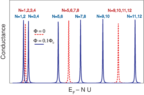
At , the conductance exhibits a four-fold symmetry due to spin and valley degeneracy. A finite flux breaks the valley degeneracy which is observable via a splitting of the conductance peaks moving with magnetic flux, see Fig. 4.
II.3 Valley qubit
We now turn to the question of how to make use of the broken valley degeneracy in order to directly address the valley degree of freedom in graphene experimentally (valleytronics valley-filter). The valley degree of freedom forms (in principle) a two-level system that can be represented by an isospin for valley and for valley . We point out that the graphene ring weakly coupled to current leads could be used to investigate the relaxation and coherence of such valley isospins.

Close to a degeneracy point of two levels belonging to different valleys (e.g. at ), Eq. (8) predicts a valley splitting of states with fixed -values controllable by flux, similar to the Zeeman-splitting for electron spins in a magnetic field. In semiconductor quantum dots, such pairs of spin-split states can be addressed via electron tunneling from/to leads weakly coupled to the quantum dot and can be used for read-out of single spins spin-read-out or measuring their relaxation () time.T1 The graphene ring could be used in very much the same way to measure the intrinsic valley isospin relaxation time in graphene as well as the valley isospin polarization.
In Fig. 5, we show the situation when some small level-mixing leads to avoided crossings of valley-split states near the degeneracy point . Such valley mixing naturally appears through boundary roughness of the ring or atomic defects in the bulk. Using the magnetic flux as a knob, we can sweep the system from a groundstate level, filled with one electron, to a superposition and further to a groundstate, see Fig. 5. Such a situation can be used to produce Rabi oscillations of the valley isospin states by tuning the system fast (non-adiabatically) from to the degeneracy point where the spin will oscillate between and in time: , where is the energy splitting at the degeneracy point.qubitH
We expect that this qubit is rather robust if intervalley scattering is weak, since time-reversal symmetry assures the (approximate) degeneracy of states from different valleys at zero flux . Indeed, the Hamiltonian Eq. (1) has the same spectrum in both valleys at zero flux, independent on the shape of the mass potential . spectrumproof This means that we do not rely on a special symmetry of the confining potential (like the circle discussed here). In addition, long-range disorder will also not lift the valley degeneracy.
II.4 Valley isospin-orbit coupling
In an open ring geometry with adiabatic contacts to leads, new interesting coherent rotations of the valley isospin occur while propagating along the ring. The linear term in in Eq. (8) can be thought of as a valley isospin-orbit coupling term, since the valley isospin couples to the orbital motion . A general incoming spinor is a superposition of spinors belonging to different valleys. Due to the valley isospin-orbit coupling, the angular momentum [determined by the incoming (continuous) energy and the applied magnetic flux via Eq. (8)] will be different for the two valleys. Consequently, the spinor in Eq. (3) will pick up different phases for the two valleys while propagating along the ring thereby rotating the valley isospin in a transport experiment.
III Spectrum for a hexagonal ring with zigzag edges
Here, we compare our analytical model with the infinite mass boundary described in Section II, to a ring with strong intervalley scattering. We numerically investigate the spectrum of a ring of hexagonal form with zigzag edges as shown in Fig. 6. (Electrical conduction through this geometry was studied in Ref. Adamringpaper.)

In a zigzag nanoribbon, the valley isospin is a good quantum number, i.e. the zigzag boundary does not mix valleys.BF Since two neighboring arms of the ring are rotated by with respect to each other, the roles of the A and B sublattices are interchanged in subsequent segments. Explicitly, this means, that if a zigzag edge is terminated on a A side, it will be terminated on a B side at a neighboring arm of the ring. Equivalently, in the reciprocal (-) space, this implies that equivalent states of subsequent zigzag nanoribbon segments are lying in opposite valleys. This necessarily induces intervalley mixing at the corners between two subsequent zigzag nanoribbon segments. This mixing is very strong in the lowest mode of the ring, where the direction of motion and the valley is tightly coupled in each arm of the hexagonal ring BF; valley-filter (the zigzag edge is therefore another example where effective TRS in a single valley is broken). An electron wave, approaching a corner of the hexagon in one valley, is either transmitted into the next arm, or reflected back into the same arm. In both cases, the valley index has to flip.
We investigate the spectrum of such a ring numerically in a tight-binding approach with Hamiltonian
| (9) |
The hopping element in the presence of a magnetic flux is where is the vector potential and are the on-site energies. The vector potential is chosen as with
| (10) |
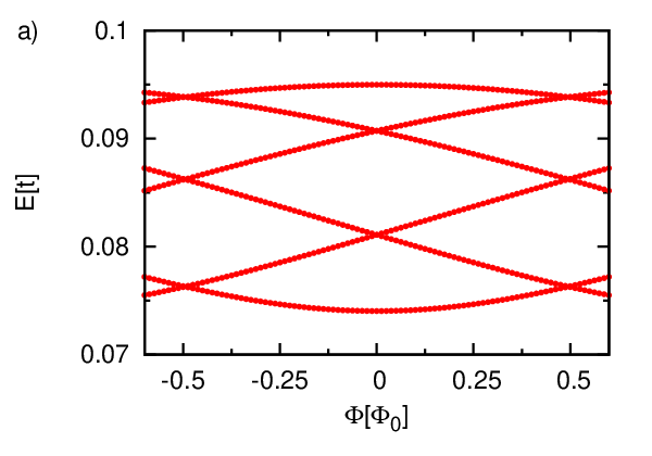
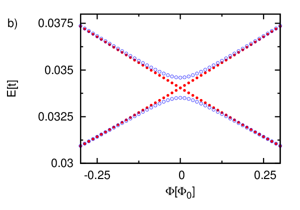
where , with for the perfect hexagon (shown in Fig. 6) and for a hexagon ring with one unit cell added to the top and bottom arm. This represents a uniform magnetic field inside the ring hole and zero outside. The spectrum as a function of magnetic flux is shown in Fig. 7 in an energy window which lies well within the lowest mode of a zigzag nanoribbon of width . modewidth A band of levels in the lowest mode is shown in Fig. 7(a). Within that mode, the spectrum follows a clear pattern which is observed for generic values of and . It consists of bands separated by energy gaps. Each band hosts six levels. The top and bottom level is non-degenerate with at zero flux (corresponding to standing waves). The other four levels are two-fold degenerate at with a broken degeneracy at finite flux. These levels correspond to right and left-going states in the ring.
We remark that this level pattern reflects the scattering off a periodic array of six scatterers subjected to periodic boundary conditions. periodic_array It is to be noted that the orbital degeneracy of the hexagonal ring can be tuned by the flux, similar to the ring with the smooth confinement discussed in Section II. If the 6-fold rotational symmetry of the ring is broken, the crossings at zero flux become slightly avoided as is shown in Fig. 7(b) (blue circles) where we have added one unit cell to two of the parallel arms of the ring (this corresponds to a length change of the arms by about 5). This shows that our results are also relevant for rings with a sligthly reduced symmetry. Note that the sensitivity of the level crossing at zero flux to the ring geometry is consistent with strong intervalley scattering where time-reversal symmetry does not protect the degeneracy at zero flux.
IV Conclusion
We have analyzed the Aharonov-Bohm effect in graphene rings. We have investigated two different ring systems – a ring with a smooth boundary (with zero or weak intervalley scattering) and a hexagonal ring with zigzag edges. For the ring with a smooth boundary, the combined effect of the effective time reversal symmetry (TRS) breaking within a single valley induced by a smooth boundary and the applied magnetic flux – breaking the real TRS – gives us at hand a controllable tool to break the valley degeneracy in such rings. We have shown that this effect of a broken valley degeneracy by flux is revealed in the persistent current and in the ring conductance. This tool could be useful for spin-based or valley-based quantum computing. The presence of a degenerate pair of levels from different valleys at zero flux is assured by time-reversal symmetry in the absence of intervalley scattering. Therefore, the proposed effect is not sensitive to the actual geometry of the ring.
We have also considered the opposite case of strong intervalley scattering by investigating numerically a hexagonal ring with lattice-terminated zigzag edges. Here, strong intervalley scattering is induced by the corners of the ring at low energies. We found that the orbital degeneracy of graphene can still be tuned by the flux similar to the ring with a smooth boundary. This effect, however, relies on a certain degree of symmetry of the ring as we show by sligthly distorting the ring. We therefore conclude that the orbital degeneracy in graphene rings can be controlled with an Aharonov-Bohm flux in rings with zero or weak intervalley scattering and in systems with strong intervalley scattering if the ring possesses an (approximate) geometric symmetry.
We acknowledge helpful discussions with A.R. Akhmerov and J.H. Bardarson. This work was financially supported by the Dutch Science Foundation NWO/FOM, the Swiss NSF, and the NCCR Nanoscience. A. Rycerz acknowledges support by the Polish Ministry of Science (Grant No. 1-P03B-001-29) and by the Polish Science Foundation (FNP).
References
- (1) For a recent review on the topic, see A.K. Geim and K.S. Novoselov, Nature Materials 6, 183 (2007).
- (2) S.V. Iordanskii and A.E. Koshelev, JETP Letters 41, 574 (1985); S.V. Morozov et al., Phys. Rev. Lett. 97, 016801 (2006); A.F. Morpurgo and F. Guinea, Phys. Rev. Lett. 97, 166804 (2006).
- (3) H. Suzuura and T. Ando, Phys. Rev. Lett. 89, 266603 (2002); D.V. Khveshchenko, Phys. Rev. Lett. 97, 036802 (2006); E. McCann, K. Kechedzhi, V.I. Fal’ko, H. Suzuura, T. Ando, and B.L. Altshuler, Phys. Rev. Lett. 97, 146805 (2006).
- (4) B. Trauzettel, D.V. Bulaev, D. Loss, and G. Burkard, Nature Physics 3, 192 (2007).
- (5) M.V. Berry and R.J. Mondragon, Proc. R. Soc. Lond. A412, 53 (1987).
- (6) Any boundary condition that does not mix the valleys can be written as , with determined by a unit vector in the plane tangent to the boundary.AKBE It holds that where ( denotes complex conjugation) is the time reversal operation in a single valley.
- (7) A.R. Akhmerov and C.W.J. Beenakker, Phys. Rev. Lett. 98, 157003 (2007).
- (8) G. Giovannetti, P.A. Khomyakov, G. Brocks, P.J. Kelly, and J. van den Brink, Phys. Rev. B 76, 073103 (2007).
- (9) S.Y. Zhou, G.-H. Gweon, A.V. Fedorov, P.N. First, W.A. de Heer, D.-H. Lee, F. Guinea, A.H. Castro Neto, and A. Lanzara, arXiv:0709.1706 (2007).
- (10) F.E. Meijer, A.F. Morpurgo, and T.M. Klapwijk, Phys. Rev. B 66, 033107 (2002).
- (11) D. Frustaglia and K. Richter, Phys. Rev. B 69, 235310 (2004).
- (12) We use with and .
- (13) In the regime , the breaking of the valley degeneracy with flux is also observed as we find numerically using Eq. (6).
- (14) L.P. Kouwenhoven, C.M. Marcus, P.L. McEuen, S. Tarucha, R.M. Westervelt, and N.S. Wingreen, in Mesoscopic Electron Transport, NATO ASI Series E, Vol. 345 (Kluwer Academic Publishers, Dordrecht, 1997) ed. by L.L. Sohn, L.P. Kouwenhoven, and G. Schön, p. 105.
- (15) We estimate meV for m and with a simple ring capacitor model with plate separation of nm and dielectric. The single-particle levelspacing for and small is eV and grows linearly with .
- (16) A. Rycerz, J. Tworzydło, and C.W.J. Beenakker, Nature Physics 3, 172 (2007).
- (17) J.M. Elzerman, R. Hanson, L.H.W. van Beveren, B. Witkamp, L.M.K. Vandersypen, and L.P. Kouwenhoven, Nature 430, 431 (2004).
- (18) R. Hanson, B. Witkamp, L.M.K. Vandersypen, L.H.W. van Beveren, J.M. Elzerman, and L.P. Kouwenhoven, Phys. Rev. Lett. 91, 196802 (2003).
- (19) Near , the spectrum is approximated by a “valley qubit”-Hamiltonian with being independent of , and and act in valley space.
- (20) This is shown as follows: If is an eigenstate of , then with the time-reversal operation in a single valley, is an (orthogonal) eigenstate of with mass potential and with the same energy. Berry But with mass potential is identical to with mass potential .
- (21) A. Rycerz and C.W.J. Beenakker, arXiv:0709.3397.
- (22) L. Brey and H.A. Fertig, Phys. Rev. B 73, 235411 (2006).
- (23) For , the energy spacing between the 1st (lowest) and 2nd mode in a zigzag nanoribbon is with . valley-filter For the ring dimensions used in Fig. 7, this gives .
- (24) R. Gilmore, Elementary Quantum Mechanics In One Dimension (The Johns Hopkins University Press, Baltimore, 2004), Chaps. 37 and 38.