Laplacian instability of planar streamer ionization fronts — an example of pulled front analysisThanks: G. Derks acknowledges a travel grant of the Royal Society, which initiated this research, and a visitor grant of the Dutch funding agency NWO and the NWO-mathematics cluster NDNS+ to finish the work. The work was also supported by a CWI PhD grant for B. Meulenbroek.
Abstract
Streamer ionization fronts are pulled fronts propagating into a linearly unstable state; the spatial decay of the initial condition of a planar front selects dynamically one specific long time attractor out of a continuous family. A stability analysis for perturbations in the transverse direction has to take these features into account. In this paper we show how to apply the Evans function in a weighted space for this stability analysis. Zeros of the Evans function indicate the intersection of the stable and unstable manifolds; they are used to determine the eigenvalues. Within this Evans function framework, a numerical dynamical systems method for the calculation of the dispersion relation as an eigenvalue problem is defined and dispersion curves for different values of the electron diffusion constant and of the electric field ahead of the front are derived. Numerical solutions of the initial value problem confirm the eigenvalue calculations. The numerical work is complemented with an analysis of the Evans function leading to analytical expressions for the dispersion relation in the limit of small and large wave numbers. The paper concludes with a fit formula for intermediate wave numbers. This empirical fit supports the conjecture that the smallest unstable wave length of the Laplacian instability is proportional to the diffusion length that characterizes the leading edge of the pulled ionization front.
Keywords: Pulled front, stability analysis, streamer ionization front, dispersion relation, wave selection of Laplacian instability.
AMS subject classifications: 37L15, 34L16, 35Q99.
1 Introduction
1.1 The streamer phenomenon, ionization fronts and Laplacian instability
A streamer is the first stage of electric breakdown in large volumes, it paves the way of sparks and lightning, but also occurs without successive breakdown in phenomena like sprite discharges above thunderclouds or in corona discharges used in numerous technical applications. Recent reviews of relevant phenomena can be found in [20, 45]. Considered as a nonlinear phenomenon, the streamer is a finger shaped ionized region that propagates by self generated field enhancement at its tip into nonionized media. It has multiple scales as described in [20]; as a consequence one can investigate a hierarchy of models on different levels of refinement that are reductions of each other, starting from the reduction from a particle to a continuum model [32] to the reduction from a continuum model to a moving boundary model [9] up to the formulation of effective models for complete multiple branched streamer trees without inner structure that are known as “dielectric breakdown models” [38, 39, 40, 7]. All these reductions are the subject of current research; the present paper analyzes the stability of fronts in the continuum model; the resulting dispersion relation provides a test case for moving boundary approximations.
Specifically, simulations of the simplest continuum model for negative streamers [15, 16, 47] have established the formation of a thin boundary layer around the streamer head. This layer is an ionization front that also carries a net negative electric charge. (Positive streamers with positive net charge occur as well, but are not the subject of the present study.) The configuration of the charge in a thin layer leads to the above mentioned field enhancement at the streamer head that creates high ionization rates and electron drift velocities and hence lets the streamer rapidly penetrate the non-ionized region. More recent numerical investigations show that the boundary layer or front can undergo a Laplacian instability that generates the streamer branch [4, 42, 36, 37]. (We remark that an additional interaction mechanism in composite gases like air somewhat modifies this picture [33] while the present analysis applies to negative streamers in simple gases like pure nitrogen or argon.)
1.2 Moving boundary layers and the transversal instability of pulled fronts
The streamer can be considered as a phenomenon where an ionized phase is separated from a non-ionized phase by a moving thin front. This concept [24, 4] implies that streamers show similar features as moving boundary problems like viscous fingers, solidification fronts propagating into undercooled liquids, growth of bacterial colonies or corals in a diffusive field of food etc. Quantitative predictions within such models require a proper understanding of the front dynamics, in particular, of their stability against perturbations in the transversal direction. This stability determines whether perturbations of the front position will grow or shrink, and on the long term whether the streamer will branch or not. As a first insight, one would therefore like to analyze the stability of planar fronts against transversal perturbations, more specifically, the growth or shrinking rate of a linear perturbation with transversal wave length .
The ionization front in the model for a negative streamer in a pure gas as treated in [15, 16, 47, 24, 25, 4, 42, 36, 37], including electron diffusion, creates a so-called pulled front that has a number of peculiar mathematical properties: (i) for each velocity , there is a dynamically stable front solution where the stability is conditional on the spatial decay of the perturbation, hence the long time dynamics is selected by the spatial decay of the initial front for (where is the spatial variable along the front); (ii) the convergence towards this front is algebraically slow in time [21, 22]; (iii) this slow dynamics is determined in the leading edge of the front that in principle extends up to and in the dynamically relevant space it will cause Fredholm integrals in the linear stability analysis to diverge, therefore curvature corrections cannot be calculated in the established manner [23], (iv) the unconventional location of the dynamically relevant region ahead of the front also requires particular care in numerical solutions with adaptive grid refinement [37]. For the calculation of the dispersion relation, which can be phrased as an eigenvalue problem for , these features pose two challenges: first, the condition on the one-dimensional dynamical stability and algebraic convergence properties, which are typical for pulled fronts, will lead to an apparently degenerate eigenvalue problem. Second, in a neighborhood of the origin, the dispersion curve is near the continuous spectrum. Hence numerical calculations of the eigenvalue problem with finite difference, collocation or spectral methods often lead to spurious eigenvalues. A dynamical systems method involving stable and unstable manifolds avoids this problem. The stable and unstable manifolds are at least two-dimensional and an exterior algebra approach is employed to calculate the manifolds accurately.
In [17, 4, 3], the treatment of pulled fronts and more-dimensional stable/unstable manifolds was circumvented by neglecting the electron diffusion that acts as a singular perturbation. In this way, the leading edge of the front together with its mathematical challenges is removed and the eigenvalue problem can be solved using shooting on the one-dimensional stable/unstable manifolds. The resulting problem is characterized by two length scales, namely the length scale of the transversal perturbation, and the longitudinal length scale of electric screening through the front that will be denoted by . The dispersion relation in this case shows a quite unconventional behavior, namely a short wave length instability whose consequences are further investigated in [35, 19]. In the present paper, we analyze the dispersion relation including diffusion, mastering the above challenges and deriving quantitative results through a combination of analytical and numerical methods.
1.3 The Evans function and pulled fronts
The Evans function is an analytic function whose zeros correspond to the eigenvalues of a spectral problem, usually a linearization about a coherent structure like a front or solitary wave. It was first introduced in [26] and generalized in [1]. In the last decade, the Evans function has been applied in the context of many problems and various extensions and generalizations have been found, see the review papers [30, 44] and references in there. One of the first uses of the Evans function in the analysis of a planar front can be found in [46], which analyzes the stability of a planar wave in a reaction diffusion system arising in a combustion model. In the current paper we will show how pulled fronts can be analyzed with the Evans function by using weighted spaces in its definition.
To define the Evans function, one writes the eigenvalue problem as a linear, first order, dynamical system with respect to the spatial variable . Along the dispersion curve , the dynamical system has a solution which is bounded for all values of . This can be phrased in a more dynamical way as: the manifold of solutions which are exponentially decaying for (stable manifold) and the manifold of solutions which are exponentially decaying for (unstable manifold) have a non-trivial intersection along the dispersion curve. The Evans function is a function of the spectral parameters and , which vanishes if the stable and unstable manifolds have a non-trivial intersection. Hence the Evans function can be viewed as a Melnikov function or a Wronskian determinant, see also [29] or references in there.
In case of a pulled front, the definition of the stable manifold, and hence the Evans function, is not straightforward. The temporal stability of the asymptotic state of the pulled front at is conditional on the spatial decay of the perturbation. So this decay condition should be included in the definition of the stable manifold, otherwise the dimension of this manifold might be too large. We will show that this condition can be built in the definition of the stable manifold by considering the stable manifold in a weighted space. The Evans function is defined by using the weighted space for the stable manifold. Hence the dispersion curve can be found as a curve of zeros of this Evans function.
1.4 Organization of the paper
In section 2, we recall the model equations and the construction and properties of planar fronts. In particular, we summarize the multiplicity, stability, dynamical selection and convergence rate of these pulled fronts. In section 3, the stability of these fronts is investigated as an eigenvalue problem for the dispersion relation of a linear perturbation with wave number . The dispersion relation depends on the far electric field and the electron diffusion as external parameters. In the stability analysis of the pulled ionization fronts, a constraint is imposed on the asymptotic spatial decay rate of the perturbations. This constraint corresponds to the decay condition for the one-dimensional stability, but has to be chosen quite subtly to avoid problems with the algebraic decay of the front solution. A consequence of the decay condition is that the eigenvalue problem (dispersion relation) is solved in a weighted space. In this weighted space, the apparent degeneracies have disappeared, the stable and unstable manifolds of the ODE related to the eigenvalue problem are well-defined and intersections of those manifolds are determined by using the Evans function. In section 3.4, dispersion relations for positive are derived numerically for a number of pairs of external parameters . The numerical implementation of the Evans function uses exterior algebra to reliably solve for the higher dimensional stable and unstable manifolds. In section 4, the numerical dispersion relation is tested thoroughly and confirmed with numerical simulations of the initial value problem for the complete PDE model for the particular values where is typically used for nitrogen [15, 16, 47, 24, 25, 4, 42, 36, 37] and is a representative value for the electric field. The later sections treat either general analytically or a larger range of numerically.
In section 5, explicit analytical asymptotic relations for the dispersion relation are derived for the limits of small and large wave numbers . For , two explicit eigenfunctions are known (which are related to the translation and gauge symmetry in the problem). These explicit solutions lead to expressions for the solutions on the stable manifold for small wave numbers. The interaction between the slow and fast behavior on this manifold leads to an asymptotic dispersion relation for small . For large wave numbers, the eigenvalue problem for the dispersion relation is dominated by a constant coefficient eigenvalue problem. An eigenvalue exists only if this constant coefficient system has no spectral gap. Using exponential dichotomies and the roughness theorem, the asymptotics of the dispersion relation is derived by a contradiction argument. In section 6, these asymptotic limits are tested on the numerical data derived in section 3. It is found that the asymptotic limit for small fits the data very well, while the asymptotic limit for large is not yet applicable in the range where is positive. After a discussion of relevant physical scales, we suggest a fit formula joining the analytical small asymptotic limit with our physically motivated guess. This formula fits the numerical data well for practical purposes and strongly supports the conjecture that the smallest unstable wave length is proportional to the diffusion length that determines the leading edge of the pulled front.
2 The streamer model and its ionization fronts
In this section we describe the streamer model and summarize the features of planar ionization fronts as solutions of the purely one-dimensional model as a preparation for the stability analysis in the dimensions transversal to the front. In particular, we recall the multiplicity of the front solutions that penetrate a linearly dynamically unstable state, and the dynamical selection of the pulled front.
2.1 Model equations
We investigate negative fronts within the minimal streamer model, i.e., within a “fluid approximation” with local field-dependent impact ionization reaction in a non-attaching gas like argon or nitrogen [24, 25, 17, 4, 42]. The equations for this model in dimensionless quantities are
| (2.1) | |||||
| (2.2) | |||||
| (2.3) |
where is the electron and the ion density, E is the electric field and is the electrostatic potential. For physical parameters and dimensional analysis, we refer to discussions in [24, 25, 17, 4, 42]. The electron current is approximated by diffusion and advection . The ion current is neglected, because the front dynamics takes place on the fast time scale of the electrons and the ion mobility is much smaller. Electron–ion pairs are assumed to be generated with rate where is the absolute value of electron drift current and the effective impact ionization cross section within a field . Hence is
| (2.4) |
For numerical calculations, we use the Townsend approximation [24, 25, 17, 4, 42]. For analytical calculations, an arbitrary function can be chosen where we assume that and therefore . We will furthermore assume that is monotonically increasing in , this is a sufficient criterion for the front to be a pulled one [22]. The electric field can be calculated in electrostatic approximation .
2.2 Two types of stationary states
It follows immediately from (2.1)-(2.3) that there can be two types of stationary states of the system, one characterized by and the other by (as implies .).
The stationary state with is the non-ionized state. As the dynamics is only carried by the electrons , there is no temporal evolution for even if the ion density has an arbitrary spatial distribution. The electric field then is determined by the solution of the Poisson equation and by the boundary conditions on . In certain ionization fronts in semiconductor devices [43], it is essential that the equivalent of does not vanish in the non-ionized region. In the gas discharges considered here, on the other hand, it is reasonable to assume that the non-ionized initial state with also has a vanishing ion density , and therefore no space charges.
The stationary state with vanishing electric field describes the ionized, electrically screened charge neutral plasma region behind an ionization front, the interior of the streamer. From the identity follows immediately, and therefore electron and ion densities have to be equal . In the absence of a field, the electrons diffuse while the ions stay put . Therefore, these densities only can stay equal if . Simulations [15, 16, 47, 24, 25, 4, 42, 36, 37] show that this occurs typically only if is homogeneous (though counter examples can be constructed).
2.3 Planar ionization front solutions
An ionization front separates such different outer regions: an electron-free and non-conducting state with an arbitrary electric field ahead of the front from an ionized and electrically screened state with arbitrary, but equal density of electrons and ions. In particular, we are interested in almost planar fronts propagating into a particle-free region (where therefore ), and we study negative fronts, i.e., fronts with an electron surplus that propagate into the electron drift direction towards an asymptotic electric field . For a planar front, it follows from that the electric field ahead of the front is homogeneous.
We assume that the front propagates into the positive direction; the electric field ahead of a negative front then is , , for . (Here is the unit vector in the -direction.) It is convenient to introduce the coordinate system moving with the front velocity . A planar, uniformly translating front is a stationary solution in this co-moving frame, hence it depends only on the co-moving coordinate , and will be denoted by a lower index 0. A front satisfies
| (2.5) |
where . This system can be reduced to 3 first order ordinary differential equations. First, due to electric gauge invariance, the system does not depend on explicitly, but only on . Using the variable instead of reduces the number of derivatives by one. Second, electric charge conservation can be rewritten in co-moving coordinates for a uniformly translating front as . Therefore it can be integrated once , . In the present problem, the space charge is and the electric current is . Furthermore, as there is a region with vanishing densities ahead of the front, the integration constant vanishes in this region, and therefore everywhere. Thus the planar front equations (2.5) can be written as
| (2.6) | |||||
where decouples from the other equations. The planar front equations imply that for all when [25].
The fronts connect the states
and the electrostatic potential connects (for ) with (for ). The ionization density behind the front and the electrostatic potential difference have to be determined for arbitrarily chosen electric field ahead of the front and for arbitrary, but sufficiently large, front velocity . (We remark that only the potential difference matters due to the gauge invariance of the electrostatic potential as one easily verifies on the equations.) The fronts can be constructed as heteroclinic orbits in a three-dimensional space as demonstrated in [25].
The diffusion constant is obviously a singular perturbation. For , the front equations can be solved analytically [25, 3], i.e., one can find explicit expressions for the particle densities , and for the front coordinate as a function of the electric field . For the negative fronts treated here, the front is continuous as function of and the limit exists and equals the value of the front at , while for positive fronts (), it is singular [25].
2.4 Multiplicity of front solutions, pulled fronts and dynamical selection
The non-ionized state with a nonvanishing electric field is linearly unstable under the temporal dynamics of the PDE (2.1)-(2.3). In fact, this spatial region ahead of the front dominates the dynamics, cf. the discussion in [25, 22]. Therefore, for fixed , there is a continuous family of uniformly translating solutions, parametrized by the velocity [24, 25, 21, 22], where
| (2.20) |
The dynamics of uniformly translating fronts with velocity are dominated by a flat spatial profile in the leading edge of the front
| (2.21) |
where velocity and decay rate are related through
| (2.22) |
and therefore for . The spatial profile (2.21) with cannot build up dynamically from some initial condition with larger ; and it will destabilize if perturbed with an initial condition with smaller , therefore such flat and fast fronts can be approached dynamically only by initial conditions with exactly the same profile (2.21) in the leading edge. For a thorough discussion of this dynamics, we refer to [22].
In practice, the continuum approximation for the electron density breaks down for very small densities in the leading edge and the initial electron distribution satisfies a decay condition of the form
| (2.23) |
if the penetrated state is really non-ionized. Therefore the velocity is called the “selected” one, because it is the generic attractor for most physical initial conditions. Mathematically speaking, the profile with velocity (the selected front) is the only profile that can build up dynamically from steeper initial conditions.
Therefore the condition (2.23) on the spatial decay of the initial electron distribution excludes all front solutions with velocity as long time attractors of the dynamics. If the criterion (2.23) is satisfied, then the selected front with speed is dynamically stable and is approached with the universal algebraic convergence rate in time [21, 22]
| (2.24) |
However, without the spatial decay condition on the initial condition, the selected front is formally not stable (although this is physically irrelevant). This will lead to specific problems and solutions in the transverse stability analysis presented in the next section.
The spatial profile of the electron distribution in the selected front is
| (2.25) |
To summarize, if the analysis is restricted to initial conditions with a sufficiently rapid spatial decay in the electron densities (2.23), then the fronts have only one free external parameter, namely the field ; it determines the asymptotic front velocity (2.20) and profile (2.25) after sufficiently long times. Furthermore, the equivariance in the system gives that the position of the front and its electrostatic potential are free internal parameters.
2.5 Full spatial profiles of the selected pulled planar front
The spatial decay behind the front will be important in the analysis as well, therefore we recall the basic behavior. For , the electron density approaches
| (2.26) |
and the electric field decays with the same exponent . For ,
| (2.27) |
was derived in [25]. For , decreases by a correction of order of , more precisely,
| (2.28) |
was proved in the appendix of [32]. The eigenvalue is given by
| (2.29) |
where both and depend on and . For small , can be approximated as
| (2.30) |
As an illustration, the spatial profiles of electron and ion density and the electric field of the selected front solution for a range of fields and diffusion constants are plotted in Figure 1.


3 Numerical calculation of the dispersion relation
First we will introduce the transversal perturbation setting and discuss an apparent degeneracy of the dispersion relation. However, it turns out that the constraint on the spatial decay of the electron density “selects” a single dispersion relation for every far field . This relation then is calculated numerically based on dynamical systems techniques involving intersections of stable and unstable manifolds. Results for different fields and diffusion constants are presented.
3.1 Linear transversal perturbations of planar fronts
Suppose that there is a linear transversal perturbation of the uniformly translating front
| (3.1) |
and similarly for and . The linearized equation for , and follows from Eqs. (2.1)-(2.3). By decomposing the perturbations into Fourier modes in the transversal directions and , by using isotropy in the transversal plane and by using a Laplace transformation in , the ansatz
| (3.2) |
can be used for each Fourier component. The resulting equation can be written as a linear first order system of ODEs, using the extra variables and . Introduce and the linear system is given by
| (3.3) | |||
In the matrix , the abbreviated notations and are used. For the terms with , we have used that , hence .
As the matrix depends on , but not on itself, the matrix is invariant under the transformation . Thus if , then also and vice versa. Therefore it is sufficient to determine the dispersion relation for and this will imply the relation for and from now on, we will use the convention that . Note that the invariance implies only that the dispersion relation will be a function of . As will be shown later, the dispersion relation is not an analytic function of near and its expansion near is linear in .
For future use, we remark that the linearization matrix does not involve any -dependent terms in the fourth and fifth row and implies that and are related by . Thus the -component of any solution of the linearized system (3.3) can be expressed as an integral
| (3.4) |
where the constants and are determined by the value of and at .
3.2 Stable and unstable manifolds and degeneracy of the dispersion relation
The linearized problem (3.3) is a spectral problem with the spectral parameters and . If the asymptotic matrices exist and are hyperbolic (i.e., no eigenvalues on the imaginary axis), then the system (3.3) has a bounded solution if and only if the unstable manifold from and the stable manifold from have a non-trivial intersection. So we will focus in this section on determining the stable and unstable manifolds.
The behavior of the unstable manifold at the back of the front is given by the asymptotic matrix
For and , this matrix has two negative and three positive eigenvalues:
| (3.5) |
Thus the unstable manifold is three dimensional. We remark that is identical to the spatial decay rate (2.29) behind the unperturbed front.
Finding the stable manifold ahead of the front is less straightforward. Normally the stable manifold ahead of the front would be characterized by the matrix . For and this matrix exists and has two positive and three negative eigenvalues:
| (3.6) |
Thus the stable manifold is three dimensional and a dimension count gives that the intersection of stable and unstable manifold is generically one dimensional. So for small values of and , a continuous family of eigenvalues seems to exist. This feature is related to the instability of the asymptotic state at , to the continuous family of uniformly translating solutions for all , and to the instability of fronts against perturbations with smaller spatial decay rate , as discussed in the previous section. The continuous family of eigenvalues for fixed wave number is eliminated by applying the analysis only to fronts with a sufficiently rapid spatial decay (2.23). This condition will be imposed in the definition of the stable manifold; it will make the spectrum discrete.
Define the scaled vector
| (3.7) |
where will be fixed later and depend on and . The freedom in the choice of is reminiscent of the fact that the decay condition holds for any , but not for . The system for is
| (3.8) |
with
Note that if , then the asymptotic matrix ahead of the front (at ) does not exist because grows linearly in according to (2.25). To get an asymptotic matrix ahead of the front, it is necessary that . In this case, the asymptotic matrix is
where . The matrix has the eigenvalues
| (3.9) |
Hence for and , there are two negative and three positive eigenvalues. Thus the stable manifold of (3.8) is two dimensional.
For the original unscaled system (3.3) this means that only the two-dimensional submanifold given by acting on the stable manifold of (3.8) is relevant for the transverse instability. This submanifold will be called the stable manifold of (3.3) from now on. With this convention, the dispersion relation is a well-defined curve and the curve is such that at , the linearized system (3.3) has a bounded solution which satisfies the spatial decay condition (2.23). Note that for both asymptotic matrices and , the eigenvalues become a degenerate eigenvalue 0 at . This leads to square root singularities and it can be expected that the dispersion relation will be a function of for is small. This will be confirmed in section 5.
3.3 The Evans function for the transverse stability problem
The occurrence of an intersection of the stable and unstable manifolds will be measured with the Evans function. Our numerical method to determine the dispersion curve as an eigenvalue problem is based on a definition of the Evans function in an exterior algebra framework and uses similar ideas as in [2, 11, 12, 8, 10, 14]. The approach of following the stable/unstable manifolds at with a standard shooting method and checking their intersection using the Evans function, works only if these manifolds are one-dimensional or have co-dimension one; in the present model, this is the case in the singular limit and a shooting method was used in [3]. Otherwise, any integration scheme will inevitably just be attracted by the eigendirection corresponding to the most unstable (stable) eigenvalue. Exterior algebra can be used to avoid this problem for higher dimensional manifolds and to preserve the analytic properties of the Evans function. Recently, a different method to calculate the Evans function for higher dimensional manifolds has been proposed in [27]. This method uses a polar coordinate approach and looks like a more suitable method for very high dimensional problems.
To calculate the evolution of the two dimensional stable and three dimensional unstable manifold in a reliable numerical way, we will use the exterior algebra spaces and , respectively. The advantage of these spaces is that in , an -dimensional linear subspace of can be described as a one-dimensional object, being the -wedge product of a basis of this space. Also, the differential equation on (or ) induces a differential equation on the spaces :
| (3.10) |
Here the linear operator (matrix) is defined on a decomposable -form , , as
| (3.11) |
and it extends by linearity to the non-decomposable elements in . General aspects of the numerical implementation of this theory can be found in [2]. The general form of the matrices and can be found in the appendix.
To determine the three-dimensional unstable manifold for , we will use (3.10) with . Since the induced matrix inherits the differentiability and analyticity of , the following limiting matrix exists:
The set of eigenvalues of the matrix consists of all possible sums of three eigenvalues of (see Marcus [34]). Therefore, for and , there is an eigenvalue of , which is the sum of the positive eigenvalues of , i.e.,
(note that the subscript “” in refers to exponentially decaying behavior at , not to the sign of , which is obviously positive). The eigenvalue is simple and has real part strictly greater than any other eigenvalue of (as is hyperbolic). We denote the eigenvector associated with as , i.e., . This vector can always be constructed in an analytic way (see [31, pp. 99-101], [10, 12, 28]). In this case it is easy to determine an explicit analytical expression for the eigenvector as is quite sparse. The unstable manifold corresponds to the solution of the linearized system (3.10) (with ) which satisfies .
The stable manifold can be determined in a similar way. As indicated in the previous section, the scaled system (3.8) will be used to determine the stable manifold. For the stable manifold with , we will use (3.10) with and the scaled matrix . As before, the asymptotic matrix
exists. Now the eigenvalues of consists of all possible sums of two eigenvalues of . Therefore, for , , has an eigenvalue , which is the sum of the negative eigenvalues of , i.e.,
As before, this eigenvalue is simple and has real part strictly less than any other eigenvalue of . The eigenvector associated with will be denoted by , i.e., The stable manifold of the scaled system (3.8) corresponds to the solution of the linearized system (3.10) (with and ) which satisfies . To get the stable manifold of the original unscaled system, the inverse scalings matrix has to be used. For arbitrary , the transformation in the wedge space is quite complicated, but we will only need the original stable manifold at . And at , the scalings matrix is the identity matrix. Hence at , the scaled stable manifold and the original stable manifold are the same and describes the stable manifold of (3.3) at .
With the stable and unstable manifold as found above, the Evans function can be defined as
| (3.12) |
Thus the Evans function is more or less the determinant of the matrix formed by a basis of the unstable manifold at and a basis of the stable manifold at . If this function is zero, then the bases are linearly dependent, hence the two manifolds have a non-trivial intersection.
We have focused on the case . For , the system is still hyperbolic, but with a two dimensional unstable manifold and a three dimensional stable manifold. The method above can be easily adapted to calculate the dispersion curve in this region too.
3.4 Numerical results on the dispersion relation with the Evans function
To calculate the Evans function numerically, first the front solution has to be determined numerically as it appears explicitly in the linearization matrix . The front is an invariant manifold connecting two fixed points of the ODE (2.6), so it can be easily determined by invariant manifold techniques or shooting, using the package DSTool [6]. Shooting works in this case as the front connects a one-dimensional unstable manifold to a three-dimensional center-stable manifold in the ODE (2.6).
After determining the fronts, the stable and unstable manifolds can be calculated by numerical integration, see e.g. [2, 10, 12]. In the numerical calculation of the stable manifold, we will use . For the stable manifold, the linearized equation on
is integrated from to , using the second order Gauss-Legendre Runge-Kutta (GLRK) method, i.e. the implicit midpoint rule. Here the scaling ensures that any numerical errors due to the exponential growth are removed and is bounded. The eigenvector can be determined explicitly as wedge product of the relevant eigenvectors of thanks to the sparse nature of this matrix.
For the unstable manifold, the linearized equation on
is integrated from to , also using the implicit midpoint rule and introducing the rescaling to remove potential exponential growth. Again, the eigenvector can be determined explicitly as wedge product of the relevant eigenvectors of .
At , the computed Evans function is (see (3.12))
| (3.13) |
For , the center-stable and the center-unstable manifold have a two-dimensional intersection, due to the translation and gauge invariance, see section 5.1 for details. In order to determine the dispersion curve, we start near and and then slowly increase and determine for which the Evans function vanishes.
The numerical errors in the calculation of the Evans function are mainly influenced by the step size used in the numerical integration with the GLRK method and errors in the numerically determined front. The numerical integration uses the step size . We have performed various checks with a decreased step size and this shows that the error in the value of for fixed is largest (order ) if is small and decreases for larger (order ). The accuracy of the front has been checked and is such that the error in the front gives a negligible error (compared to the error due to the error in the step size) in the value of . It turns out that the scheme is not very sensitive to errors in the front (at least for the and values considered).
In the following sections, we will present data for the dispersion curve for varying electric field and diffusion coefficient . A more detailed discussion of the data, relation with analytical asymptotics and some empirical fitting can be found in section 6.
3.4.1 Varying the electric field ahead of the front
First we consider how the dispersion curve depends on the electric field ahead of the front, while the diffusion coefficient is fixed to . In Figure 2(a), the dispersion curve is shown for , and . The figure shows that the shape of the dispersion curve stays similar, but the scales of and increase when increases. The dispersion curves can be characterized by the maximal growth rate and the corresponding wave number where as well as by the wave number with that limits the band of wave numbers with positive growth rates.


3.4.2 Varying the diffusion coefficient
Next we consider the effect of varying the diffusion coefficient , while keeping the electric field ahead of the front fixed at . In [3] it is shown that if diffusion is ignored (), the dispersion curve stays positive and is monotonically increasing to the saturation value for . Our numerics shows that if diffusion is present, this is not the case anymore. This is not surprising as diffusion is a singular perturbation. In Figure 2(b), the dispersion curve is shown for , and ; the data for is taken from [3]. It shows that the growth rate has a maximum if diffusion is present and becomes negative for larger than some . Furthermore for decreasing diffusion , the maximal growth rate moves upward towards the saturation value for . This suggests that some features of the dispersion curve behave regularly in , in spite of the fact that is a singular perturbation. For example, for a finite wave number interval, the limit of the dispersion curves for exists and is the curve for . However, the asymptotic profile for large values of the wave number is obviously singular in . This duality can also be found in the front itself: the velocity and the profile of the ionization density and the electric field of the uniformly translating negative front depend regularly on , while the profile of the ionization density is singular, as discussed in section 2.4 and shown in Fig. 1.
4 Numerical simulation of the perturbed initial value problem
In the previous section, we have determined the dispersion relation for transversal perturbations of ionization fronts as a temporal eigenvalue problem of the PDE system linearized about the uniformly translating planar front. Since we are dealing with pulled fronts (cf. sections 1 and 2.4), the problem is unconventional: both the velocity of the uniformly translating planar front and the dispersion relation of its transversal perturbations are unique only if the spatial decay constraint (2.23) is imposed. Furthermore a longitudinally perturbed planar front approaches its asymptotic profile and velocity algebraically slowly in time (2.24). Therefore it is worthwhile to test the predicted dispersion relation on direct numerical simulations of the corresponding initial value problem.
In this section, we will therefore simulate the temporal evolution of a perturbed planar front by numerically solving the full nonlinear PDEs (2.1)-(2.3), and we will determine the dispersion curve from a number of simulations with perturbations with different wave vectors . This is done for far field and diffusion constant .
To determine the instability curve with a simulation of the full PDE, we parametrize the evolution of a perturbed planar front with wave number as
| (4.1) |
If is small enough, the solution is in the linear regime, and can be determined from the evolution of the perturbation after has relaxed to some time independent function. Therefore in the numerical simulations, we choose for each wave number in such a manner that is large enough to extract meaningful growth rates and that is small enough that the dynamics at the final time is still well approximated by the linearization about the planar front.
Furthermore, an appropriate choice of the initial condition reduces the initial transient time during which in the co-moving frame still explicitly depends on time . Ideally, such an initial condition is of the form etc., where is a solution of the linearized system (3.3). To find an approximation for , we use that the instability acts on the position of the front, i.e., we write the perturbed front as . Therefore we choose and the initial condition as
| (4.2) |
As is a solution of the linearized system for , this choice will be very efficient for small values of and require longer transient times for larger .
To solve the full 2D PDE, the algorithm as described in [4, 42] is used, while adaptive grid refinement as introduced in [37] was not required. For fixed , the PDE with initial condition (4.2) is solved on the spatial rectangle . The length of the domain in the transversal -direction, , is such that exactly 5 wave lengths fit into the domain, i.e., , and periodic boundary conditions are imposed in this direction by identifying with . On the boundaries in the longitudinal -direction, Neumann conditions for the electron density are imposed. The potential is constant far behind the front and the electric field is constant far ahead of the front; therefore for the potential , the Dirichlet condition is imposed at , and the Neumann condition at accounts for the far field ahead of the front.
The amplitude of the perturbation is conveniently traced by the maximum of the electron density
| (4.3) |
evaluated across the front. The reason is as follows. First, Figure 1 shows the spatial profiles of planar fronts for different electric fields and illustrates that for fixed , the maximum of the electron density as well as the asymptotic density behind the front strongly depend on the field immediately ahead of the front, where for a planar front the close and the far field are identical: . Second, the modulation of the front position leads to a modulation of the electric field immediately before the front (cf. discussion in section 5.2); therefore as a function of is modulated as well.


An example of as a function of the transversal coordinate for a fixed time is plotted in Fig. 3(a). The amplitude of the wave modulation is determined by the Fourier integral
In Figure 3(b) we plot against time for . Note that is close to (see Figure 2(a) and Table 1) where the growth rate vanishes, , therefore the growth rate in the present example is small and particularly sensitive to numerical errors.
Figure 3(b) shows an initial temporal transient before steady exponential growth is reached (where exponential growth manifests itself as a straight line in the logarithmic plot). This is typically observed for the larger -values (); as said before, this is related to the fact that the function in the initial condition (4.2) is not optimal. For , there are less transients as for small values of .
To determine the growth rate , a least squares algorithm is used to fit the best line through the data points , and the initial transient time is ignored for larger values of . For each value of , the growth rate is determined with various choices of . The resulting growth rate is indicated in Figure 4 with crosses X and the error bars are related to the various choices of .

Fig. 4 also shows the dispersion relation for determined with the dynamical systems method in the previous section 3.4; these numerical results are denoted with and can now be compared with the results of the initial value problem from the present section. Around the maximum of the curve, the agreement between the numerical results of the two very distinct methods is convincing. For larger values of , the differences increase, but the error bars of the initial value problem results increase as well. Furthermore, the plotted error bars are an underestimation as they only account for the errors discussed above that emerge from the choice of the initial condition and from the time interval of evaluation and therefore from possible initial transients and from a possible transition to nonlinear behavior. Additional errors can be due to the numerical discretization and time stepping of the s themselves. We therefore conclude that the two results agree within the numerical error range of the initial value simulations over the whole curve.
5 Analytical derivation of asymptotic limits for and
Having determined the dispersion relation numerically for different values of electric field and diffusion constant in section 3, and having tested the correctness of the eigenvalue calculation against numerical solutions of the initial value problem in section 4, we now will analytically derive asymptotic expressions for the dispersion relation for small and large values of the wave modes . It will be shown that these asymptotic limits are
In doing so, we mathematically formalize and generalize the derivation of the small asymptotic limit that was presented in [3] for the singular limit , and we correct the result proposed in [5]; and we also rigorously derive the large asymptotic limit, in agreement with the form proposed in [5].
5.1 Analysis for the asymptotic limit
Translation invariance and electrostatic gauge invariance give two explicitly known bounded solutions of the linearized system (3.3) at and . These are
Note that is a solution of the linearized system (3.3) for and arbitrary.
From the asymptotics of (3.3) for at , we see that the only exponentially decaying solution at is given by . This solution is related to the only positive eigenvalue (see (3.5)). For , the solution , hence this solution is not exponentially decaying for . However, it is easy to obtain an explicit exponentially decaying solution at , this is .
From the eigenvalues in (3.5) it follows that for and , the three-dimensional unstable manifold at involves one eigenfunction with a fast exponential decay (related to the eigenvalue ) and two eigenfunctions with a slow exponential decay (related to the eigenvalues and ). Similarly, from the eigenvalues in (3.9), it follows that the two-dimensional stable manifold at involves one eigenfunction with a fast exponential decay (related to the eigenvalue ) and one eigenfunction with a slow exponential decay (related to the eigenvalue ). Recall that the stable manifold is defined as a subset of the full stable manifold to account for the spatial decay condition (2.23).
We focus on approximating an exponentially decaying solution on the stable manifold. As we have seen above, in lowest order, this solution is
To determine the next order, we will use the slow behavior of the asymptotic system and write
The second term on the right-hand side () is an approximation of the slow behavior on the stable manifold, while the other three terms are related to the fast decay. Because of the slow decay, the expansion is only valid on a -interval with , hence shouldn’t be too large.
Substitution of these expressions into the linearized system (3.3) gives that and have to satisfy
By analyzing the unperturbed system, we can find a particular solution of the first equation. The front solution satisfies
Differentiating this system with respect to gives
Hence
The asymptotic behavior of is
| (5.1) |
The polynomial growth in the -component will need to be canceled by the behavior of the other terms which involve and hence will give a relation between and .
In fact, the -components of the linearized system (3.3) for any or can be expressed by the integral equation (3.4). For all solutions on the stable manifold, the limit is well-defined, so we can write the -components on the stable manifold as
In the integral, must satisfy the decay condition (2.23) on the stable manifold and hence will have fast exponential decay. Furthermore, from (3.3), it can be seen that . As the term inside the integral has fast exponential decay, we get that on the stable manifold and has fast exponential decay too. Thus the integral in the expression for has fast exponential decay for large. Since , we get on the stable manifold for small and -values not too large, say (hence )
The exponentially decaying solution on the stable manifold is given by
and the arguments above show that the order contribution in the -components is given fully by and that does not contribute to those components at this order. So it follows that the polynomial growth in the -component of as given by (5.1) has to be canceled by the -component in , i.e., or
| (5.2) |
and given in Eq. (2.20). Equation (5.2) establishes the small limit of the dispersion relation .
5.2 A physical argument for the asymptotic limit
There is also a physical argument for the asymptotic limit (5.2) that generalizes the calculation in section IV.C of reference [3] to nonvanishing . For , the wave length of the transversal perturbation is the largest length scale of the problem. It is much larger than the inner longitudinal structure of the ionization front. On the length scale , the front can therefore be approximated by a moving boundary between ionized and non-ionized region at the position
| (5.3) |
and the local velocity of this perturbed front is
| (5.4) |
The electric field in the non-ionized region is determined by , where is the solution of the Laplace equation together with the boundary conditions; these are for fixing the field far ahead of the front and making the ionization front almost equipotential. (Due to gauge invariance the constant potential can be set to zero.) The solution of this problem is
| (5.5) |
here is the electric field extrapolated onto the boundary from the non-ionized side.
As the perturbation is linear, the front is almost planar . Therefore it will propagate with the velocity (2.20) of the planar front in the local field . Inserting from (5.5) and expanding about , we get
| (5.6) |
Comparison of (5.6) and (5.4) immediately gives the dispersion relation (5.2), that generalizes the result that was derived in [3] for the singular limit .
5.3 Analysis for the asymptotic limit
The asymptotic limit for is derived by a contradiction argument. We will suppose that is large and that is positive, but not small, i.e.,
| (5.7) |
and show that this does not allow for bounded solutions. With the assumptions above on and , the dominant contributions in the matrix on the whole axis are
| (5.8) |
Here the three entries , and are necessary for a nonvanishing determinant.
We want to use the Roughness Theorem [13] for exponential dichotomies to show that for large and not close to , the exponential dichotomy of the constant coefficient ODE is close to the exponential dichotomy of the full system. So first we recall the definition of an exponential dichotomy, which gives projections on stable or unstable manifolds.
Definition 1 ([13])
Let be a matrix in , , and , , or . Let be a solution matrix of the linear system
| (5.9) |
The linear system (5.9) is said to possess an exponential dichotomy on the interval if there exist a projection and constants and with the following properties:
An extension for PDEs of this definition can be found in [41].
The Roughness Theorem for exponential dichotomies states the following.
Theorem 2 (Roughness Theorem [13])
Consider the system
| (5.10) |
with a hyperbolic matrix and . Then for all there exists a such that for all matrix functions with , the system (5.10) has an exponential dichotomy on (and ) with its dichotomy exponents and projections -close to those of (in the norm).
A constant coefficient linear system does not have bounded solutions. So if the exponential dichotomy of the linearized system (3.3) is close to the one of the constant coefficient system with the matrix as in (5.8), the linearized system (3.3) does not have bounded solutions either. We will show that this is the case if and satisfy the assumptions (5.7).
First we introduce some scaling and coordinate transformations. Define the small parameter and the scaled spatial variable, the transformation matrix and transformed vector
Now (3.3) can be written as
| (5.11) |
with
and
The eigenvalues and eigenvectors of the constant coefficient matrix are
If , then the matrix is not hyperbolic at . However, this problem is not fundamental as it is known that there is a hyperbolic splitting in the full problem (see section 3.2) and there is a spectral gap between the positive and negative eigenvalues, even if is close to zero. The spectral gap disappears if (or ) and in this case the following arguments will not work. The spectral gap allows us to define a weight function which moves the spectrum away from the imaginary axis. To be specific, define
Then satisfies the ODE
| (5.12) |
and the spectrum of is bounded away from zero for all small (as long as is not small). The system
| (5.13) |
has an exponential dichotomy with projection such that the range of is the span of all eigenvectors of the negative eigenvalues and the kernel of is the span of all eigenvectors of the positive eigenvalues. Then is the projection on the stable subspace of the linear system (5.13) and is the projection on the unstable subspace.
Clearly the matrix is uniformly bounded for all and small. Thus applying the Roughness Theorem 2 gives that for small there is an exponential dichotomy for the system (5.12) on with projection onto the stable subspace such that is -close to for all . And similarly, there is an exponential dichotomy for the system (5.12) on with projection onto the unstable subspace such that is -close to for all . Thus the range of is -close to the range of and the range of is -close to the range of , so the range of and the range of have only a trivial intersection for small.
As the weight function has been chosen such that no eigenvalue crosses the imaginary axis, it affects only the value of the dichotomy exponentials, not their sign, nor the stable and unstable manifolds. Hence the stable and unstable manifolds of (5.11) have a trivial intersection only. And the same holds for the stable and unstable manifolds of (3.3), as the only difference between the systems (5.11) and (3.3) is a scaling. So it can be concluded that the linear system (3.3) does not have any bounded solutions for small ( large) and not close to .
If is close to , i.e., , then the matrix has a positive and negative eigenvalue of order and the spectral gap will disappear in the limit . So the roughness theorem can not be applied anymore and no conclusion about bounded solutions can be drawn.
The arguments above show that only if , there is a possibility for bounded solutions to exist. As the dispersion curve indicates a bounded solution of the ODE (3.3), this implies that for near zero, hence large, the dispersion curve is
| (5.14) |
So far we have used that . If one considers the linear system (3.3), an edge of the continuous spectrum is given by the curve . However, one should include the decay condition (2.23), i.e., the scaling (3.7). For any the edge becomes . By taking the limit for , we see that the curve is an edge of the continuous spectrum. Thus with the decay condition, either the dispersion curve satisfies or it ends at the continuous spectrum.
6 Physically guided fits to the numerical dispersion relations
In section 3 we have derived dispersion relations for a number of fields and diffusion constants by numerically solving an eigenvalue problem, we have confirmed these calculations by a numerical solutions of the initial value problem in section 4, and we have derived analytical asymptotic limits to these dispersion relations in section 5. This sets the stage for comparing the numerical results to the analytical asymptotic limits and for deriving physically guided empirical fits to the numerical dispersion curves where the analytical asymptotic limits are not applicable. The small -data derived in section 3.4 and the analysis of section 5.1 are shown to be consistent in section 6.1. After showing in section 6.2 that a simple cross-over formula joining the asymptotic behavior of the small wave numbers with the asymptotic behavior of the large wave numbers is not satisfactory, we give a data collapse, empirical fits and arguments on relevant scales in section 6.3.
6.1 Testing the small asymptotic limits
First the asymptotic relation (5.2) for small is tested on the numerical results. Beyond the results visible in the plots of figure 2, the numerical dispersion relation for and was evaluated carefully for small values of , and the result is shown in a double logarithmic plot in Figure 5 that zooms in on the small behavior. Also plotted is the analytical asymptotic limit (5.2). The comparison between numerical data and analytical asymptotic limit is convincing in the range of small .
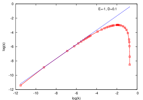
6.2 Testing both asymptotic limits
It is quite suggestive to join the small asymptotic limit (5.2) with the large asymptotic limit (5.14) into one cross-over formula
| (6.1) |
A formula similar to was suggested in [5], but with a different prefactor instead of . However, we now will confirm once more the correctness of the prefactor , and we will show that the large asymptotic limit is not yet applicable in the range of positive growth rates .
If (6.1) holds, then the dispersion relation for the rescaled variable as a function of the rescaled wave number becomes . Therefore the formula (6.1) can easily be tested on the numerical data from figure 2 by plotting them in rescaled variables and with appropriate values for and for each curve. The result is shown in Fig. 6, together with the parabola . The plot illustrates that the asymptotic limit (5.2) indeed is a very good fit to all data for small .
For larger , the curves differ quantitatively. In particular, vanishes for between 0.014 and 0.035 for the numerical dispersion curves while the formula (6.1) predicts this to happen for . Also the maximum of the dispersion curve is never higher than 0.0027 for the numerical data while formula (6.1) predicts 0.25. Of course, this is not in contradiction with the analytical results in Section 5.3 for large . Rather it says that the positive part of the dispersion curve lies completely in the range of small , where the asymptotic limit for large is not applicable. We conclude that cross-over formula (6.1) is not an appropriate fit for the numerically derived dispersion relations.

6.3 Data collapse, relevant length scales, empirical fits and conjectures
We finish this section with a data collapse and arguments on relevant scales that guide empirical fits.
6.3.1 Data collapse
First, we investigate whether the numerical data for different and can be collapsed onto one curve. This is done by determining the maximum of the dispersion curve and the wave number where the growth rate vanishes, , from the numerical data for each pair . In figure 7 all curves are plotted as and with their respective and . The plot shows that the curve shapes are very similar, but they do not coincide completely. For example, there seems to be a small drift in the position of the maximum.

6.3.2 Relevant length scales and the case
In a second step, we investigate which physical or mathematical mechanisms can suppress the growth rate for much smaller values of than suggested by the large asymptotic limit (5.14). In a first overview, there are three length scales in the problem. The transversal perturbation is characterized by its wave length . In the longitudinal direction, the front is characterized by two length scales, the electric screening length and the diffusion length , cf. Fig. 1,
| (6.2) |
For vanishing diffusion , the diffusion length vanishes, and the screening length has to be compared to the wave length of the perturbation; in [3] it was shown that it determines the cross-over from the small to the large asymptotic limit of the dispersion relation:
The actual curve for and is given in figure 2(b), where we remark that the form
| (6.6) |
for positive real reproduces the asymptotic limits (6.3.2), but does not fit the full numerical curve for satisfactorily for any power . The functional form of (6.6) will serve below as an inspiration for our empirical fits for .
Searching for why (6.6) does not properly fit the data, one realizes that there are actually two different definitions of the screening length possible:
| (6.7) |
with from (2.29). The dimensions of both quantities are the same, and they approach each other if is constant in a large part of the integration interval ; this is the case with the Townsend approximation for . Otherwise, characterizes the slopes of the fields near the discontinuity of [3], while characterizes the decay (2.26) of the fields far behind the front for . The analysis in [3] shows that linear perturbations with wave numbers couple to the inner local structure of the front and are dominated by , while smaller could couple to the larger spatial structure characterized by , this conjecture will be tested on the numerical data below and asks for future analysis.
6.3.3 Scales and fits for
When diffusion is included, the diffusion length emerges as another length scale in the front. As illustrated in figure 1, instead of the discontinuous electron density in the front for , a diffusive layer of width (2.25) builds up in the leading edge. While increases, the dispersion relation decreases as shown in figure 2(b). As the diffusive layer is the main new feature of the front for , it is plausible that the different behavior of is created within this boundary layer. The physical mechanism is that diffusion can smear perturbations of short wave length out, hence suppressing their growth. This process mainly takes place in the diffusive layer because gradients are largest in this region. This idea has inspired an attempt in [5] to calculate by local analysis within the diffusion layer. In principle, such an approach combined with proper matched asymptotic expansions could work. However, the calculation in [5] was intrinsically inconsistent [18], disagrees with our asymptotic limit for small and therefore fits the numerical results even worse than formula (6.1), cf. Fig. 6.
We have tested whether the diffusion length plays a role in the dispersion relation by plotting the numerical data from Fig. 2 this time for the rescaled variables over . The result is shown in Figure 8. It shows that the numerical dispersion curves are well approximated by
| (6.8) | |||||
| (6.9) |
The numerical evidence from Fig. 8 summarized in (6.9) together with the physical explanation above suggest the following conjecture.
Conjecture 1
The largest unstable wave number of the Laplacian instability is proportional to the inverse diffusion length.
We remark that the data gives , while the cross-over formula (6.1) would suggest that , highlighting again its inadequacy for intermediate values. Figure 8 also shows that the value of the wave number for which the maximum of the dispersion curve is attained, lies in the range of to .


The data in Figure 8 suggest an empirical formula of the form (for )
| (6.10) |
where the parameter will depend on the external parameters and . The factor creates the correct asymptotic limit (6.8) for . The factor creates the non-trivial zero of the dispersion relation at (6.9). The form of the numerator is inspired by (6.6), and the proper asymptotic limit (6.3.2) for large and would be reached for . Obviously, the empirical formula (6.10) is not valid in the asymptotic range where and where the asymptotic behavior is given by .
The functional form of formula (6.10) is supported by the following observation. If one calculates the maximum of (6.10), it follows that , independently of the value of . (The number 1/4 directly stems from the factor 4 in .) This relation indeed fits the numerical curves quite well, therefore the factor 4 is supported twice independently. Relevant numerical data for this and other fits is collected in Table 1.
The value for is less obvious. The empirical formula (6.10) gives the following relation between and the maximum of curve
The empirical values for those quotients are given in Table 1.
The limit of and suggests , but the fit is unconvincing (cf. also the discussion for above). However, we found that fits the data reasonably well. Formula (6.10) with this value of together with the numerical data are visualized in Figure 8(a). The fit is quite good for the lower two curves, the upper two display some discrepancies. The main problem is the value of with a relative error between and , while the position of has a relative error as low as to . As , another possible fit is , it is displayed in Figure 8(b). The fit is quite good for the upper two curves, but now the fit has some discrepancies for the lower two curves. And the value of has a larger error between and while the position of has a much smaller error of only to . Obviously, these observations ask for further analytical investigation. Note finally the striking relation between and the value of for larger values of the electric field in Table 1. As a basis for future work, all characteristic numerical data is collected in this table.
| 0.080(1) | 0.05190(2) | 0.1695(15) | 0.647(1) | 1.6305(15) | |
| 0.35(4) | 0.144(1) | 0.25(4) | 0.45(4) | 0.60(4) | |
| 1.575(15) | 0.4825(5) | 0.875(25) | 1.595(1) | 2.397(1) | |
| 4.56(56) | 3.35(3) | 3.60(65) | 3.57(33) | 4.01(27) | |
| 1.12 | 1.38 | 2.70 | 6.28 | 11.9 | |
| 1.12 | 1.38 | 2.52 | 5.77 | 11.0 | |
| 6.07 | 1.92 | 3.48 | 6.40 | 9.51 | |
| 0.37 | 0.37 | 0.61 | 0.82 | 0.90 | |
| 0.148 | 0.144 | 0.638 | 2.832 | 7.169 | |
| 0.13 | 0.10 | 0.23 | 0.45 | 0.60 | |
| 49.5 | 15.6 | 17.2 | 23.4 | 31.5 | |
| 55.5 | 21.6 | 21.7 | 27.0 | 34.8 | |
| 0.260(3) | 0.252(1) | 0.251(5) | 0.249(1) | 0.252(1) | |
| 0.0118(2) | 0.0196(1) | 0.0193(2) | 0.0175(1) | 0.0155(1) | |
| 1.9(2) | 0.78(1) | 0.8(2) | 1.1(1) | 1.3(1) | |
| 0.28(7) | 0.288(4) | 0.27(9) | 0.28(5) | 0.26(4) | |
| 40(6) | 17.7(1) | 21(2) | 22(2) | 31(2) | |
| 48.1(4) | 22.5(1) | 23.0(1) | 26.8(1) | 32.3(1) |
7 Conclusion and outlook
In this paper, we have found dispersion curves for negative streamer ionization fronts by numerically solving an eigenvalue problem, we have verified this prediction on the numerical solution of an initial value problem, we have derived analytical expressions for the asymptotics of the curve for large and small wave lengths, and we have presented a physically motivated fit formula to the numerical curves for intermediate wave lengths. The investigation is of interest for two reasons: because pulled fronts like these ones are mathematically challenging to investigate, and because explicit predictions on the linear stability of ionization fronts help to interpret numerical and experimental observations of propagating and branching streamer discharges.
The ionization front is a pulled front, i.e., the front is part of a family of traveling waves, which propagate into a temporally unstable steady state. For the dynamics with one spatial variable, most traveling waves in this family are attractors only for waves with exactly the same asymptotic decay profile. The exception is the pulled front, which has the steepest decay of all waves in the family and is an attractor for waves with a sufficiently fast decay (therefore excluding the slower decay rates for the other traveling waves in the family). The instability of the state ahead of the front and the related spatial decay condition imply that only a submanifold of the stable manifold in the transverse instability problem is relevant for the transverse instability analysis. This submanifold is identified by introducing a weighted solution space that excludes solutions with a too slow decay rate. We have integrated the relevant stable submanifold and unstable manifold numerically with a dynamical systems method to calculate the dispersion curve. This method of finding the dispersion curve does not use any details of the streamer model, except that it has a pulled front. The definition of a submanifold of the stable manifold and the subsequent numerical integration of this stable submanifold and the unstable manifold are ideas that can be applied to pulled fronts in other systems, too.
It is interesting to see that the band of unstable wave numbers seems to be limited by a multiple of the decay rate that characterizes the leading edge of the pulled ionization front; though the evidence up to now is only numerical. As such behavior is physically reasonable, the next step would be to derive it analytically, e.g., by a local analysis in the diffusive layer and matched asymptotic expansions. Such an expansion could be based on the limiting case where the diffusion length is much smaller than the screening length .
The calculated dispersion curves also contribute to understanding the stability of actual streamers. Two- and three-dimensional time dependent simulations [4, 42, 36, 37, 33] of the streamer model introduced in section 2 show them to become unstable and branch. Can the unstable wave lengths of this branching be related to the unstable band of wave lengths of the present calculation? Furthermore, if the inner front structure is approximated by a moving boundary [35, 19], how is the calculated dispersion relation of transversal perturbations to be taken into account? It will also be interesting to see whether the dispersion relation calculated for the present fluid model is also applicable to the corresponding particle model [32].
Finally, we mention that the extension of the streamer model with photo-ionization as an additional reaction term [33] in composed gases like air requires an extension of the present analysis as nonlocal interaction terms play a role.
Appendix A Matrices in exterior algebra spaces
In this appendix, we give explicit expressions for the matrices acting on the exterior algebra space for . Let be the standard basis for . Then an induced basis on is given by
The matrix can be associated with a complex matrix with entries such that
| (A.1) |
where, for any decomposable , . Let be an arbitrary matrix with complex entries,
| (A.2) |
then takes the explicit form
where .
In a similar way, the matrix can be associated with a complex matrix. First we define an induced basis on by
The matrix for has entries such that
| (A.3) |
where, for any decomposable , . If is given by (A.2), then takes the explicit form
where .
Acknowledgments
We thank Björn Sandstede for helpful discussions on the roughness theorem. We thank Willem Hundsdorfer and René Reimer for advice and help with the simulations in section 4.
References
- [1] J. Alexander, R. Gardner & C.K.R.T. Jones. A topological invariant arising in the stability analysis of traveling waves, J. Reine Angew. Math. 410 (1990), pp. 167–212.
- [2] L. Allen & T.J. Bridges. Numerical exterior algebra and the compound matrix method, Numerische Mathematik 92 (2002), pp. 197–232.
- [3] M. Arrayás and U. Ebert. Stability of negative ionization fronts: Regularization by electric screening?, Phys. Rev. E 69 (2004), article no. 036214 (10 pages).
- [4] M. Arrayás, U. Ebert and W. Hundsdorfer. Spontaneous branching of anode-directed streamers between planar electrodes, Phys. Rev. Lett. 88 (2002), article no. 174502 (4 pages).
- [5] M. Arrayás, M.A. Fontelos, and J.L. Trueba. Mechanism of branching in negative ionization fronts, Phys. Rev. Lett. 95 (2005), article no. 165001 (4 pages).
- [6] A. Back, J. Guckenheimer, M.R. Myers, F.J. Wicklin & P.A. Worfolk. DsTool: Computer assisted exploration of dynamical systems, Notices Amer. Math. Soc. 39 (1992), pp. 303-309.
- [7] A.D.O. Bawagan. A stochastic model of gaseous dielectric breakdown, Chem. Phys. Lett. 281 (1997), pp. 325–331.
- [8] K.B. Blyuss, T.J. Bridges and G. Derks. Transverse instability and its long-term development for solitary waves of the (2+1)-dimensional Boussinesq equation, Phys. Rev. E 67 (2003), article no. 056626 (9 pages).
- [9] F. Brau, A. Luque, B. Meulenbroek, U. Ebert, L. Schäfer. Construction and test of a moving boundary model for negative streamer discharges, preprint: arXiv:0707.1402 .
- [10] T. Bridges, G. Derks & G. A. Gottwald. Stability and instability of solitary waves of the fifth-order KdV equation: a numerical framework, Physica D 172 (2003), pp. 190–216.
- [11] L.Q. Brin. Numerical testing of the stability of viscous shock waves, Math. Comp. 70 (2001), pp. 1071–1088.
- [12] L.Q. Brin & K. Zumbrun. Analytically varying eigenvectors and the stability of viscous shock waves, Seventh Workshop on Partial Differential Equations, Part I (Rio de Janeiro, 2001). Mat. Contemp. 22 (2002), pp. 19–32.
- [13] W. Coppel. Dichotomies in stability theory. Lecture Notes in Mathematics. Springer, 1978.
- [14] G. Derks & G. A. Gottwald. A robust numerical method to study oscillatory instability of gap solitary waves, SIAM J. Appl. Dyn. Sys. 4 (2005), pp. 140–158.
- [15] S.K. Dhali, P.F. Williams. Numerical simulation of streamer propagation in nitrogen at atmospheric pressure, Phys. Rev. A 31 (1985), pp. 1219–1221.
- [16] S.K. Dhali, P.F. Williams. Two-dimensional studies of streamers in gases, J. Appl. Phys. 62 (1987), pp. 4696–4707.
- [17] U. Ebert and M. Arrayás, Pattern formation in electric discharges, pp. 270-282 in: Coherent Structures in Complex Systems (eds.: Reguera, D. et al), Lecture Notes in Physics 567 (Springer, Berlin 2001).
- [18] U. Ebert and G. Derks, Comment on [5], 1 page submitted to Phys. Rev. Lett.
- [19] U. Ebert, B. Meulenbroek, L. Schäfer. Rigorous stability results for a Laplacian moving boundary problem with kinetic undercooling, SIAM J. Appl. Math. 69 (2007), pp. 292–310.
- [20] U. Ebert, C. Montijn, T.M.P. Briels, W. Hundsdorfer, B. Meulenbroek, A. Rocco, E.M. van Veldhuizen. The multiscale nature of streamers, Plasma Sources Science and Technology 15 (2006), pp. S118–S129.
- [21] U. Ebert, W. van Saarloos, Universal algebraic relaxation of fronts propagating into an unstable state and implications for moving boundary approximations, Phys. Rev. Lett. 80 (1998), pp. 1650–1653.
- [22] U. Ebert, W. van Saarloos. Front propagation into unstable states: Universal algebraic convergence towards uniformly translating pulled fronts, Physica D 146 (2000), pp. 1–99.
- [23] U. Ebert, W. van Saarloos. Breakdown of the standard Perturbation Theory and Moving Boundary Approximation for “Pulled” Fronts, Phys. Rep. 337 (2000), pp. 139–156.
- [24] U. Ebert, W. van Saarloos and C. Caroli, Streamer Propagation as a Pattern Formation Problem: Planar Fronts, Phys. Rev. Lett. 77 (1996), pp. 4178–4181.
- [25] U. Ebert, W. van Saarloos and C. Caroli, Propagation and Structure of Planar Streamer Fronts, Phys. Rev. E 55 (1997), pp. 1530–1594.
- [26] J.W. Evans. Nerve axon equations IV. The stable and unstable impulse, Indiana Univ. Math. J. 24 (1975), pp. 1169–1190.
- [27] J. Humpherys and K. Zumbrun. An efficient shooting algorithm for Evans function calculations in large systems. Physica D 220 (2006), pp. 116–126.
- [28] J. Humpherys, B. Sandstede and K. Zumbrun. Efficient computation of analytic bases in Evans function analysis of large systems. Numerische Mathematik 103 (2006), pp. 631-642.
- [29] T. Kapitula, The Evans function and generalized Melnikov integrals. SIAM J. Math. Anal. 30 (1999), pp. 273-297.
- [30] T. Kapitula and B. Sandstede. Eigenvalues and resonances using the Evans function. Discrete and Continuous Dynamical Systems 10 (2004), pp. 857-869.
- [31] T. Kato. Perturbation Theory for Linear Operators. Second Edition, Springer Verlag: Heidelberg (1984).
- [32] C. Li, W.J.M. Brok, U. Ebert, J.J.A.M. van der Mullen. Deviations from the local field approximation in negative streamer heads, J. Appl. Phys. 101 (2007), article no. 123305 (14 pages).
- [33] A. Luque, U. Ebert, C. Montijn, W. Hundsdorfer. Photoionisation in negative streamers: fast computations and two propagation modes, Appl. Phys. Lett. 90 (2007), article no. 081501 (3 pages).
- [34] M. Marcus. Finite Dimensional Multilinear Algebra, Part II, Marcel Dekker: New York (1975).
- [35] B. Meulenbroek, U. Ebert, L. Schäfer. Regularization of moving boundaries in a Laplacian field by a mixed Dirichlet-Neumann boundary condition: exact results, Phys. Rev. Lett. 95 (2005), article no. 195004 (4 pages).
- [36] C. Montijn, U. Ebert, W. Hundsdorfer. Numerical convergence of the branching time of negative streamers, Phys. Rev. E 73 (2006), article no. 065401 (4 pages).
- [37] C. Montijn, W. Hundsdorfer, U. Ebert. An adaptive grid refinement strategy for the simulation of negative streamers, J. Comp. Phys. 219 (2006), pp. 801–835.
- [38] L. Niemeyer, L. Pietronero, H.J. Wiesman. Fractal Dimension of Dielectric Breakdown, Phys. Rev. Lett. 52 (1984), pp. 1033–1036.
- [39] L. Niemeyer, L. Ullrich, N. Wiegart. The mechanism of leader breakdown in electronegative gases, IEEE Trans. Electr. Insul. 24 (1989), pp.309–324.
- [40] V.P. Pasko, U.S. Inan, T.F. Bell. Mesosphere-troposphere coupling due to sprites, Geophys. Res. Lett. 28 (2001, pp. 3821–3824.
- [41] D. Peterhof, B. Sandstede and A. Scheel. Exponential dichotomies for solitary-wave solutions of semilinear elliptic equations on infinite cylinders. Journal of Differential Equations, 140 (1997) pp. 266–308.
- [42] A. Rocco, U. Ebert and W. Hundsdorfer. Branching of negative streamers in free flight, Phys. Rev. E, 66 (2002), article no. 035102(R) (4 pages).
- [43] P. Rodin, U. Ebert, W. Hundsdorfer, I.V. Grekhov. Superfast fronts of impact ionization in initially unbiased layered semiconductor structures, J. Appl. Phys. 92 (2002), pp. 1971–1980.
- [44] B. Sandstede. Stability of travelling waves. In: Handbook of Dynamical Systems II (B Fiedler, ed.). North-Holland (2002), pp 983-1055.
- [45] S.M. Starikovskaia. Plasma assisted ignition and combustion, J. Phys. D: Appl. Phys. 39 (2006), pp. R265–R299.
- [46] D. Terman. Stability of Planar Wave Solutions to a Combustion Model, SIAM J. Math. Anal. 21 (1990), pp 1139-1171.
- [47] P.A. Vitello, B.M. Penetrante, J.N. Bardsley. Simulation of negative streamer dynamics in nitrogen, Phys. Rev. E 49 (1994), pp. 5574–5598.