Testing Radiative Neutrino Mass Generation at the LHCPreprint:
Abstract:
We investigate in detail a model that contains an additional singlet and triplet scalar fields than the Standard Model (SM). This allows the radiative generation of Majorana neutrino masses at two-loop order with the help of doubly charged Higgs bosons that arise from the extended Higgs sector. The phenomenology of the Higgs and neutrino sectors of the model is studied. We give the analytical form of the masses of scalar and pseudoscalar bosons and their mixings, and the structure of the active neutrino mass matrix. It is found that the model accommodates only normal neutrino mass hierarchy, and that there is a large parameter space where the doubly charged Higgs can be observed at the Large Hadron Collider (LHC), thereby making it testable at the LHC. Furthermore, the neutrino-less double beta () decays arise predominantly from exchange processes involving the doubly charged Higgs, whose existence is thus unmistakable if decays are observed. The production and decays of the doubly charged Higgs are analyzed, and distinct and distinguishing signals are discussed.
Keywords:
Neutrino Mass, Doubly Charged Higgs, LHC1 Introduction
The origin of small active neutrino masses remains one of the most challenging problem in physics. The small neutrino masses generated through the seesaw mechanism is popularly viewed as heralding new physics at scales larger than GeV, and thus provide a window to Grand Unified Theories (GUTs) with or without supersymmetry. Crucial to the construction is the introduction of heavy Standard Model (SM) singlet fermions commonly known as sterile neutrinos.
Recently, the idea of extra spatial dimensions together with brane world scenarios offers a very different perspective to the question of neutrino masses. Here their smallness results from either the suppression factors associated with the relatively large extra dimensions, or from the small overlap between the wave functions of the sterile neutrinos in the extra dimensions.
It is interesting to note that these different perspectives can be incorporated into a single framework in brane world scenarios; a recent discussion can be found in [1]. However the existence of sterile neutrinos is required in both constructions which, along with the value of their masses, are all important questions by themselves. To date the best information on light sterile neutrinos comes from cosmological considerations; direct experimental tests are very challenging due to the fact that they have no SM interactions.
It is well known that the masses of active neutrinos can be generated without sterile right-handed (RH) neutrinos via quantum loop effects. Without the RH states there are no Dirac couplings of the SM lepton doublet to the Higgs fields, and consequently the active neutrinos can only have Majorana masses. The prototype model was constructed in [2] where there is an extended Higgs sector, and the gauge symmetry is that of the SM. Crucial to the construction was the use of an singlet Higgs field with a nontrivial hypercharge. Unfortunately the model gives rise to bimaximal neutrino mixings which is disfavored by the most recent neutrino data (for a recent review see [3]). More realistic neutrino masses can be obtained using doubly charged Higgs fields [4].
In our construction, we keep the SM gauge group and extend the Higgs sector by adding both an triplet and a doubly charged singlet field. We also postulate that lepton number violating effects take place only in the scalar potential, while the rest of the Lagrangian respect lepton number. A brief discussion of our model has already appeared in [5] where we showed how naturally small neutrino masses can arise from just two-loop radiative corrections. In this paper we will give a detail discussion of rich scalar phenomenology of the model. In particular the signals at the Large Hadron Collider (LHC) are investigated.
The rest of the paper is organized as follow. In Sec. 2 we describe in detail our model. We work out the constraints on the vacuum expectation value and other parameters that control the mass of the two physical doubly charged Higgs bosons . We show that at least one of the doubly charged Higgs can have mass at the electroweak scale if we demand the theory be perturbative up to the TeV scale. In Sec. 3 we discuss in detail the phenomenology of the neutrino sector in our model. We examine closely the neutrino mass matrix and the constraints from the oscillation data. We show that normal hierarchy arises naturally in our model, and we place constraints on the neutrino-lepton Yukawa couplings. Lastly, we discuss the implications these constraints have on the decays of nuclei in our model. In Sec. 4 we discuss the phenomenology of the doubly charged Higgs production at the LHC, and their decays. We show that the decay pattern of the doubly charged Higgs in our model can be very different, and can therefore be used to distinguish our model from others that also contain doubly charged Higgs. Sec. 5 contains our conclusions.
2 A minimal model with radiative neutrino mass generation.
The model is based on the SM gauge symmetry with an extended Higgs sector and minimal matter content. Group theory dictates that only singlets and triplets are allowed for the generation of Majorana masses for the neutrinos. Besides the SM Higgs doublet given by
| (1) |
we introduce a complex triplet Higgs represented by a matrix
| (2) |
as well as a complex singlet scalar . The subscripts denote the weak hypercharges of the fields as given by the relation . The most general potential for the scalar fields is given by
| (3) |
One can assign a lepton number 2, and a lepton number 0. Then terms in the square brackets at the end of Eq. (2) contain lepton number violating interactions. We will take both , to be positive so that spontaneous symmetry breaking (SSB) takes place. Minimizing the potential gives us the VEVs: and .
With the additional fields and , two new Yukawa terms can be constructed that are allowed by the gauge symmetry. The first is , which is lepton number conserving. Here are family indices and is a lepton singlet. The second is that violates lepton number, which we assume not to occur at the tree level ** * There are several ways to naturally suppress the Yukawa couplings of . One way is to embed the model in a 5-dimensional set-up and compactify the extra dimensions on an orbifold . The lepton and Higgs fields are then assigned with different orbifold parities to forbid the term while still allows the term. Another way is to further extend the Higgs sector by including a second Higgs doublet and then employ an appropriate discrete symmetry. The term will be generated radiatively after symmetry breaking, but is small.. The absence of this term frees one from having to put in by hand a very small value of in the eV range that plagues other Higgs models of neutrino masses. Adding in the SM terms and the covariant derivatives of and we have a complete renormalizable model.
From Eq. (2) it can be seen that the various Higgs fields will mix among themselves. In particular, the pair and will mix that give rise to two physical neutral scalars, and , and the pair and will mix with one combination that is eaten by the boson to leave a physical pseudoscalar . Similarly for the charged states and , one combination will be eaten by the bosons leaving only a pair of singly charged scalars. Finally the weak eigenstates and will also mix to form physical states and , with the mixing angle denoted by , and masses and respectively. All the masses and mixing angles are free parameters in our model, which we can use to replace some of the parameters in . They are to be determined experimentally. In summary, the physical spin 0 particles consist of a pair of singly charged bosons, , two pairs of doubly charged bosons and , a pair of Higgs scalars and , and a pseudoscalar .
The value of is constrained by the electroweak phenomenology. After the electroweak symmetry breaking, the and bosons pick up masses at the tree level given by
| (4) |
where we have used standard notations, and the tree level relation holds. From the Particle Data Group (PDG) we have [6] and GeV [7]. This implies that GeV. We will see below that this is a controlling scale for the neutrino masses.
In the limit where , the model conserves lepton number, and is thus technically natural. Since is a dimensionless coupling, it is expected to be of order unity () so that perturbation is valid, which is assumed throughout this paper. The value of is important in setting the scale of lepton number violation. It enters in the conditions for minimizing the scalar potential :
| (5) | ||||
| (6) |
where and . Taking to be of the electroweak scale and , the interesting limiting cases are:
- A.
: The minimum conditions, Eq. (5), can be naturally satisfied without fine tuning between the parameters if .
- B.
: To satisfy the minimum conditions, is required. This appears to be unnatural although not forbidden.
- C.
: The minimum conditions can only be satisfied by tuning the dimensionful and/or the dimensionless couplings. We will not consider this case.
For convenience define . Then Case A and B correspond to and respectively. Qualitatively, we see that is more natural in our model. We will therefore concentrate mostly in this region of the parameter space below.
We now turn to the masses of the physical scalar and pseudoscalar particles in our model. The mass of the singly charged Higgs boson is given by
| (7) |
For , we expect the charged Higgs to have mass in the 100 to 1000 GeV range.
For the two doubly charged scalars, their masses are given by
| (8) |
where the state takes the upper sign, and
| (9) |
Note that () is a mass parameter for the singlet and should not be confused with the physical mass. As such it is in general not constrained.
Consider now Case A. In the limit where is large (), we have from Eqs. (8) and (9):
| (10) | ||||
| (11) |
We see in this limit, saturates to an m-independent value, , which is also its maximal value for a given set of model parameters. On the other hand, increases as , which means the state will be too heavy to be of interest to the LHC in the large limit.


In Fig. 1 we plot the maximal value of as a function of , with and set to 4 GeV. The coupling is set to , the upper limit under which perturbation is expected to be valid. In Fig. 2 we plot as a function of for three different values of , with all dimensionless couplings kept perturbative. We see clearly here the saturation of at large values of . Figs. 1 and 2 show that the mass range of the state is well within the reach of the LHC, its existence is thus a testable feature of our model at the LHC.
Note that if we take the opposite limit where , two weak scale doubly charged scalars are possible. For example, if we take , , , and , we get GeV and GeV. However, this will not hold in Case B. In this case the state will be heavy with mass above a TeV, while the state remains at the weak scale.
The doubly charged scalars form a two-level system in which the mass and weak eigenstates are related by
| (12) |
The mixing angle is a measurable physical parameter. It is given by
| (13) |
where , and are those given in Eq. (9). For Case A, if , the mixing can be large and close to maximal. But if , the mixing will be small, which is expected since the two states are widely split. For case B, large mixing can be achieved only if a cancellation occurs between the various parameter in Eq. (2).
We now turn to the three physical neutral scalar bosons in our model. The pseudoscalar has mass given by
| (14) |
Note that if , becomes a Majoron.
The masses of the neutral scalars and again have the general form
| (15) |
where the state takes the upper sign, and
| (16) |
The physical neutral scalars also form a two-level system in which the mass and weak eigenstates mix, with the mixing angle, given by
| (17) |
It can be seen that is of order for both Case A and B.
For Case A, and can both be light and almost degenerate. If they are lighter than half the Z boson mass they will contribute to its invisible width [8]:
| (18) |
where the notation is standard. Demanding that this contributes less than 150 MeV to the invisible width we obtain . For Case B, all the neutral bosons have weak scale masses and the above limit does not apply. However, we still expect and to be close in mass.
We summarize our findings on the masses of the scalar and pseudoscalar bosons in our model:
- A.
: The mass of is expected to be greater than GeV if TeV. But if is much larger than that, the mass of will saturate to a constant value which is at most GeV; the states are expected to be very heavy in the large limit. The singly charged Higgs has a mass at the weak scale that is -independent. The masses of neutral Higgs-like bosons are also of the weak scale. Being the would-be Majoron, provides a bound on : .
- B.
: Here, only the mass of is expected to be at the weak scale. All the other scalars with the exception of (which is mostly a SM Higgs boson) will be too heavy to be of interest at the LHC, since their masses are controlled by .
3 Neutrino phenomenology and constraints
3.1 Two-loop neutrino masses and neutrino oscillations
A feature of our model is that neutrino masses are generated at the two-loop level, and the crucial couplings are the Yukawa terms. It is well known that the Yukawa couplings of to fermions are diagonalized by a biunitary transformation effected via and such that the charged leptons are mass eigenstates. Clearly, applying this transformation does not in general diagonalize . Hence we expect flavor violating couplings between families of RH leptons and the physical states. †† † In the following we assume that the charged leptons are in the mass basis, and so . For notational simplicity we will drop the prime henceforth. Thus in general, the decay modes such as must occur. The coupling of to fermions, on the other hand, is similar to SM but scaled by a factor .

The active neutrino mass matrix can now be calculated. The leading contribution is given by the two-loop Feynman diagram depicted in Fig. 3. After a standard but lengthy calculation we find
| (19) |
where . The integral is given by
| (20) |
The integral can be evaluated analytically as in [9]. Note that there is a generalized GIM mechanism at work here. This can be seen clearly in the limit [10]:
| (21) |
We see that not only is the neutrino mass two-loop suppressed, there is also a helicity suppression from the charged lepton masses, whose origin can be clearly seen from Fig. 3(b). It is clear that the internal lepton lines must have mass insertions since only couples to RH leptons. As a result, will be vanishingly small. This has important consequences in decays as well as the choice of signatures for the detection of these scalars at the LHC.
Explicitly, the neutrino mass matrix is given by
| (22) |
where
| (23) |
and gives a qualitatively estimate of the overall scale of active neutrino masses. Now for normal hierarchy, the neutrino mass matrix has the following structure
| (24) |
where , and . Comparing Eq. (3.1) to Eq. (24), we see there is a qualitatively agreement.


We plot the behavior of as a function of and in Fig. 4. The range of parameters used is applicable to Case A. We see that overall, the neutrino mass increases as the mass difference of the two doubly charged scalar increases. In Fig. 5 we plot the behavior of for parameter range applicable to Case B. In both cases we expect neutrino masses to be in the sub-eV range.
We proceed next to examine how the neutrino oscillation data can constrains our model. Neutrino oscillations depend on the difference of mass-squared, hence we will focus on accordingly. Since the eigenvalues of are in general complex, and it is customary to separate out a phase matrix, we write
| (25) |
where is the neutrino mixing matrix [11] and in standard notation is the same as the quark mixing matrix [6], whereas is the Dirac phase. For normal hierarchy, we have , , and . Oscillation experiments currently place limits on the following relevant parameters [3]:
| (26) |
Using Eqs. (3.1) and (25) and the oscillation data we can get six constraints on the elements of . From the first row of we obtain
| (27) |
Since the phases involved are unknown, we do not get lower bounds for these quantities. As will be seen below, the bounds given in Eq. (27) are very loose compared to that found from rare muon and decays. The remaining three constraints are more stringent relatively, and they came by demanding a good fit to normal hierarchy:
| (28) | ||||
| (29) | ||||
| (30) |
Using Eqs. (29) and (30), we plot in Fig. 6 the allowed parameter space for and , with set to eV. ‡‡ ‡ In plotting Fig. 6, we have used the fact that , which we show below.

3.2 Rare muon and decays
The doubly charged Higgs bosons lead to many lepton number violating processes. Since no such signals were found in current experiments, they lead to very strong constraints on the Yukawa couplings. In the following, we work out these constraints.
- A.
Muonium anti-muonium conversion
The effective Hamiltonian is given by the exchange at tree level:
(31) where is the reduced mass of the pair of doubly charged Higgs given by
(32) The current experimental limit [6] gives
(33) - B.
Effective , , contact interactions
The effective Hamiltonian for Bhabha scattering is
(34) The bounds are
(35) - C.
Rare decays and its counterparts
These decays can all be induced at the tree level and thus provide the most stringent limits on the Yukawa couplings. For , the branching ratio is given by
(36) with similar equations for decays. The constraints impose by the data is given by
(37) - D.
Radiative flavor violating charged leptonic decays
We consider here rare radiative decays of and . The fact that they are not seen to a very high precision make them of paramount importance for probing the physics of lepton flavor violation. The branching for is calculated in [12] using an effective theory approach:
(38) with obvious substitutions for decays. The limits are given by
(39)
Comparing the sets of constraints we find that Eq. (C) gives the strongest limits. Although the limits from contact interactions, Eq. (B), are less stringent, they are useful nonetheless as they constrain individual couplings. We illustrate in Fig. 7 how and are restricted by both contact and rare decay experiments for a chosen value of the reduced mass GeV.

It is also interesting to compare the limits from the rare decays with that from neutrino oscillations. We plot in Fig. 8 the parameter space allowed in this case for and , with eV and GeV. Other comparisons are less instructive.

3.3 decays of nuclei
In our model, decays of nuclei are induced by the exchanges of virtual bosons and Majorana neutrino as depicted in Fig. 9.

The quark level amplitude due to neutrino exchanges is given by §§ § In our order of magnitude estimation, we have ignored spinor and kinematic factors, as well as factors from nuclear physics.
| (42) |
where is the average momentum of the light neutrino exchanged. For notational simplicity we will drop the subscript for the mass matrix. Typically, GeV which reflects the long range nature of light particle exchanges. Note that there is a cancellation between the contributions from and , which is characteristic of a two level system.
The doubly charged Higgs exchange amplitude is given by
| (43) |
where is given by Eq. (3.1). We estimate that . The smallness of this ratio is due to the fact that in our model, is suppressed not only by a two-loop factor, it is also suppressed by the electron mass factor coming from the doubly charged scalar coupling. We conclude that if seen, decays of nuclei will be due to the existence of doubly charged Higgs at the weak scale. This can be tested at the LHC, and is the subject of next section. Since there is no conclusive evidence for these decays, we use it to set a limit of . The result is displayed in Fig. 10. It can be seen that the limit here is comparable to that from the contact interactions.

4 Doubly Charged Higgs at the LHC
4.1 Production of the doubly charged Higgs
A central ingredient in our neutrino mass generation is the two doubly charged Higgs, . We have argued that if not both, at least one of the doubly charged Higgs is well within reach of the LHC. Without loss of generality, we will take to be this (lighter) state, and focus on its production and decay below.
Now the doubly charged Higgs, , have no direct couplings to the quarks, which is characteristic of models with doubly charged scalars. However, they do couple to the SM gauge bosons. Thus at the LHC, will be produced predominantly via the fusion processes, as illustrated in Fig. 9(a) (the d-quark is replaced by the u-quark for ), and the Drell-Yan (DY) annihilation processes,
| (44) |
The relevant gauge-scalar couplings are given by ¶¶ ¶ For couplings with , , .
| (45) |
where , , and .
We calculate the production cross sections numerically using the CalcHEP package [13], which allows an easy implementation of our model. The calculations are leading order, and are done in unitary gauge. The cross sections are calculated for pp collisions in the center-of-mass (CM) frame with energy TeV, and CTEQ6M [14] parton distributions functions are used to fold in the cross section for the hard partonic production processes.
From Eq. (4.1) we see that the only model parameters the production cross section explicitly depend on are and the mixing angle . The dependence on all other model parameters are implicit through the dependence on the mass, , as given in Eq. (8). The choice we made in our calculations is thus to set
| (46) |
and vary by varying . Note that with this choice, is independent of , and thus . For the SM parameters, we take GeV, and .

We plot in Fig. 11 the production cross section for from fusion and Drell-Yan pair annihilation as a function of . Note that QCD corrections are expected to increase the DY production cross section by a factor of about 1.25 at next-to-leading order [15]. The CalcHEP results are checked with that calculated from Pythia [16], and are found to be consistent.
Except for the mixing angle factors and , the coupling of to the weak gauge bosons are the same as that of to the , bosons in the left-right symmetric model [17], while the couplings to photon is the same in both models. Thus, the results for the cross section should agree once the scaling factors are taken into account. Comparing the results of our model to that of Refs. [18, 19], we find good agreements.
We see from Fig. 11 that DY pair production is dominant compared to the single production channel via fusion for the whole range of masses in our model. This is a robust feature in the production of the doubly charged Higgs at hadron colliders in many models. This is because the virtual photon exchange is the same for all models and only the exchange term is model dependent, which is subdominant. The relative magnitude of production via WW fusion compared to the DY pair production can thus be used to distinguish between the different models containing the doubly charged Higgs.
4.2 The decay of
At the leading order, there are six decay channels possible for :
| (47) |
Kinematically, mode (4) and (6) are not allowed in our model, while the availability of the rest depends on the value of the scalar boson masses. The coupling for mode (2) has been given in Eq. (4.1), for mode (1), (3) and (5) the couplings are given by
| (48) |
where for respectively.
The leptonic decays are kinematically the most favorable mode of decay for the doubly charge Higgs, , and this is a universal feature in any model that contains them. The leptonic decay width has a very simple form given by
| (49) |
Note that in our model, the final state charged leptons are right-handed. Hence in principle, helicity measurements can be used to distinguish between our model and those whose doubly charged Higgs coupling only to left-handed leptons (see e.g. [20, 21, 22, 23, 24]).
From the discussion above, it is not unreasonable to take (except for , which is constrained to be ten times smaller). Thus, provided the mixing angle between the doubly charged Higgs bosons, , is not too small, one can expect spectacular signals from like-sign dileptons such as , and , that are directly produced from .
The channel opens up once . Its decay width is
| (50) |
which is proportional to . Given that is small, and is of order the electroweak scale, whether the leptonic or mode dominates depends on the value of the mixing angle .
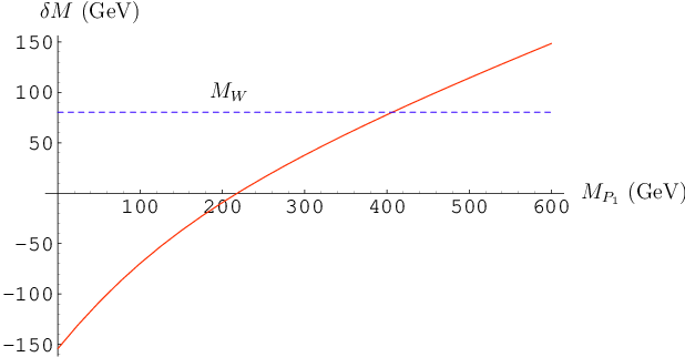
The mode opens up once the mass difference, , where is the mass of the singly charged Higgs boson, is greater than . From Eq. (7), we see that if is to be of interest at the LHC, needs to be order unity (the validity of perturbation theory constrains to be less than ). This implies that , and in Fig. 12 we plot as a function of for GeV. We vary the same way as detailed in Sec. 4.1, with the same choice of parameters, Eq. (46). For this choice, the decay channel opens up once GeV.
The decay width for the mode is given by
| (51) |
where . With a dependence of and no suppression coming from factors of , the mode is expected to dominate over the mode once it becomes available. Note that the singly charged Higgs decays primarily into rather than fermion pairs, which is the dominant decay mode for the usual charged Higgs originating from SM doublets.
In general, the three-body decay mode , , is expected to be relatively suppressed by the three-body phase space when compared to the two-body modes. However, since the couplings do not depend on , if , it may become important compared to the lepton and modes.
The masses of the neutral pseudoscalar and scalar bosons, , are given by Eqs. (14) and (15). Here too, is required to keep the neutral bosons at electroweak scale. Note that once is fixed, and are governed by independent sets of parameters. Below, we will choose as the representative three-body mode, which has the least and simplest model dependence compared to the neutral scalar cases. The difference in the decay widths would come in only as ratios of masses, and from the neutral mixing angle factors, and .

For the choice GeV, GeV, and the mode opens up once GeV. Since there is no known closed form for the phase space of general three-body decays, we calculate the three-body decay widths numerically using CalcHEP as a function of . We display the result and compared with all the allowed two-body modes listed in Eq. (4.2) in Fig. 13. We work in the small mixing scenario where , since for , the results are qualitatively that of the left-right symmetric models [17].
There are several noteworthy features. First, despite the phase space advantage, the suppression of the lepton mode by the factor is such that the mode is never negligible for , and dominating for even for small values of . Next as discussed above, the mode dominates over both the lepton and modes, and does so almost at once after it becomes kinematically available. Moreover, even if one were to push to the perturbative limit of , the mode would still become dominant soon above its threshold. Lastly, and perhaps most interestingly, the three-body mode dominates over the lepton mode when (suppression by ), and is significant relative to the mode and even overtakes it at large values of (suppression by ).
These are features that are not shared by other doubly charged Higgs models, and will serve to distinguish our model from them at the LHC.
5 Conclusion
We have given a detail study of the phenomenology of a model where Majorana neutrino mass is induced radiatively at two-loop. This is made possible by extending the Higgs sector of the SM, and the new structure involves a triplet and a doubly charged singlet field. Lepton number is violated only in the scalar sector by a hard and a soft term. When these two terms are set to zero, the model conserves lepton number, and is technically natural.
Since the active neutrinos masses are two-loop effects due to new physics at the TeV scale, the model is testable at the LHC. In our study, we have focused on the production and decays of the doubly charged Higgs bosons. We find it is possible in the enlarged Higgs sector parameter space to have always at least one doubly charged Higgs with mass GeV. Furthermore, in much of the parameter space, two doubly charge Higgs can be expected to have masses within reach of the LHC. We find that Drell-Yan mechanism is the dominant production mechanism, with single production from fusion coming into play only for masses greater than 600 GeV. This is common to most doubly charged Higgs models. We find cross sections ranging from fb without including QCD effects, which typically cause an enhancement by a factor of 1.25.
The decays of the doubly charged Higgs are potentially the best way of differentiating between the different doubly charged Higgs models. We find that with reasonable values of the Yukawa couplings, the leptonic decays are not always dominant despite being kinematically favorable. Nevertheless, decay modes producing directly same sign dilepton pairs such as , , and , are distinctive and unmistakable. Moreover, since the doubly charged Higgs only couples to RH leptons in our model, their decays into a pair of tauons offer opportunities for helicity measurements. Another interesting feature of the doubly charged Higgs decays is that three-body modes involving the neutral scalar and pseudoscalar bosons can become as important as the two-body modes, particularly when the mixing between the doubly charged Higgs is small.
The model we studied here can only accommodate the normal hierarchy for the active neutrino mass matrix. It predicts that the first element to be very small. Moreover, decays of nuclei can still occur via the exchange of doubly charged Higgs. This give rise to the interesting situation whereby if such decays are seen, the doubly charged Higgs will also be seen at the LHC, and vice versa. If the neutrino mass hierarchy turns out to be other than the normal hierarchy, neutrino masses are not generated by the model we studied.
Acknowledgments.
We thank Dr. D. Axen for kindly sharing with us his knowledge and insights on Pythia, and Dr. G. Azuelos for useful discussions. This work is supported in part by the National Science Council of R.O.C. under Contract No. NSC-95-2112-M-007-059-MY3, and by the Natural Science and Engineering Council of Canada.References
- [1]
K. R. Dienes, E. Dudas and T. Gherghetta,
Light neutrinos without heavy mass scales: A higher-dimensional seesaw mechanism,
Nucl. Phys. B 557 (1999) 25 [hep-ph/9811428];
S. J. Huber and Q. Shafi, Seesaw mechanism in warped geometry, Phys. Lett. B 583 (2004) 293. - [2]
A. Zee,
A Theory Of Lepton Number Violation, Neutrino Majorana Mass, And Oscillation,
Phys. Lett. B 93 (1980) 389 [Erratum-ibid. B 95 (1980) 461];
Charged Scalar Field And Quantum Number Violations, Phys. Lett. B 161 (1985) 141. - [3] G. L. Fogli, E. Lisi, A. Marrone and A. Palazzo, Global analysis of three-flavor neutrino masses and mixings, Prog. Part. Nucl. Phys. 57 (2006) 742 [hep-ph/0506083].
- [4]
A. Zee,
Quantum Numbers Of Majorana Neutrino Masses,
Nucl. Phys. B 264 (1986) 99;
K.S. Babu, Model of ’Calculable’ Majorana Neutrino Masses, Phys. Lett. B 203 (1988) 132. - [5] C. S. Chen, C. Q. Geng and J. N. Ng, Unconventional neutrino mass generation, neutrinoless double beta decays, and collider phenomenology, Phys. Rev. D 75 (2007) 053004 [hep-ph/0610118].
- [6] W. M. Yao et al. [Particle Data Group], Review of particle physics, J. Phys. G 33 (2006) 1.
- [7] O. Stelzer-Chilton [for the CDF Collaboration], First Run II Measurement of the W Boson Mass with CDF, hep-ex/0706.0284.
- [8] M. C. Gonzalez-Garcia and Y. Nir, Implications Of A Precise Measurement Of The Z Width On The Spontaneous Breaking Of Global Symmetries, Phys. Lett. B 232 (1989) 383.
- [9]
J. van der Bij and M. J. G. Veltman,
Two Loop Large Higgs Mass Correction To The Rho Parameter,
Nucl. Phys. B 231 (1984) 205;
K. L. McDonald and B. H. J. McKellar, Evaluating the two loop diagram responsible for neutrino mass in Babu’s model, hep-ph/0309270. - [10] K. S. Babu and C. Macesanu, Two-loop neutrino mass generation and its experimental consequences, Phys. Rev. D 67 (2003) 073010 [hep-ph/0212058].
- [11]
B. Pontecorvo,
Neutrino experiments and the question of leptonic-charge conservation,
Sov. Phys. JETP 26 (1968) 984;
Z. Maki, M. Nakagawa, and S. Sakata, Remarks on the unified model of elementary particles, Prog. Theor. Phys. 28 (1962) 870. - [12] M. Raidal and A. Santamaria, – conversion in nuclei versus : An effective field theory point of view, Phys. Lett. B 421 (1998) 250
- [13] A. Pukhov et al., CompHEP: A package for evaluation of Feynman diagrams and integration over multi-particle phase space. User’s manual for version 33, hep-ph/9908288; A. Pukhov, CalcHEP 3.2: MSSM, structure functions, event generation, batchs, and generation of matrix elements for other packages, hep-ph/0412191.
- [14] J. Pumplin, D. R. Stump, J. Huston, H. L. Lai, P. Nadolsky and W. K. Tung, New generation of parton distributions with uncertainties from global QCD analysis, J. High Energy Phys. 0207 (2002) 012 [hep-ph/0201195].
- [15] M. Mühleitner and M. Spira, Note on doubly charged Higgs boson pair production at hadron colliders, Phys. Rev. D 68 (2003) 117701
- [16] T. Sjostrand, S. Mrenna and P. Skands, PYTHIA 6.4 physics and manual, J. High Energy Phys. 0605 (2006) 026 [hep-ph/0603175].
- [17] J. F. Gunion, J. Grifols, A. Mendez, B. Kayser and F. I. Olness, Higgs Bosons In Left-Right Symmetric Models, Phys. Rev. D 40 (1989) 1546.
- [18] K. Huitu, J. Maalampi, A. Pietila and M. Raidal, Doubly charged Higgs at LHC, Nucl. Phys. B 487 (1997) 27 [hep-ph/9606311].
- [19] G. Azuelos, K. Benslama and J. Ferland, Prospects for the search for a doubly-charged Higgs in the left-right symmetric model with ATLAS, J. Phys. G 32 (2006) 73 [hep-ph/0503096].
- [20] J.A. Coarasa, A. Méndez, and J. Solà, Higgs triplet effects in purely leptonic processes, Phys. Lett. B 374 (1996) 131.
- [21] A. G. Akeroyd and M. Aoki, Single and pair production of doubly charged Higgs bosons at hadron colliders, Phys. Rev. D 72 (2005) 035011 [hep-ph/0506176].
- [22] A. G. Akeroyd, M. Aoki and Y. Okada, Lepton Flavour Violating tau Decays in the Left-Right Symmetric Model, hep-ph/0610344.
- [23] A. Hektor, M. Kadastik, M. Muntel, M. Raidal and L. Rebane, Testing neutrino masses in little Higgs models via discovery of doubly charged Higgs at LHC, hep-ph/0705.1495.
- [24] T. Han, B. Mukhopadhyaya, Z. Si and K. Wang, Pair Production of Doubly-Charged Scalars: Neutrino Mass Constraints and Signals at the LHC, hep-ph/0706.0441.