跳到论文正文
W Papers独立论文阅读器 arXiv:0706.1793 论文正文 计算阅读时间 · 0%
引用这篇论文根据当前论文元数据生成,正式投稿前建议核对。


License: Assumed arXiv.org perpetual non-exclusive license
arXiv:0706.1793v2 [hep-th] 26 Jun 2007

UNIVERSIDADE DE SANTIAGO DE COMPOSTELA

Departamento de Física de Partículas

The beta function of gauge theories
at two loops in differential renormalization

Tesis presentada para optar al grado de Doctor en Física.

César Seijas Naya

Santiago de Compostela, febrero 2007.

Agradecimientos

Si sale, sale. Y si no sale
hay que volver a empezar.
Lo demás son fantasías
Edouard Manet

En un trabajo que ha llevado tanto tiempo, es normal el tener un montón de gente a la que agradecerle el apoyo prestado para terminarlo. Espero que no se me olvide nadie, ya que como dijo Quevedo: “el agradecimiento es la parte principal de un hombre de bien”.

En primer lugar, tengo que agradecer al profesor Javier Mas la oportunidad que me ha brindado de poder realizar esta tesis doctoral. Entre otras muchas cosas, y dejando a parte toda la física que he aprendido con él, me gustaría destacar su apoyo en las diferentes circunstancias por las que he pasado durante todo este tiempo, así como el haber intentado enseñarme a tener la visión crítica necesaria para llevar a cabo una investigación. También me gustaría agradecer la ayuda que me han brindado los profesores Manuel Pérez-Victoria y Jose Ignacio Latorre. A Manuel tengo que darle las gracias por haber compartido conmigo su amplio conocimiento de renormalización diferencial y simetrías, y por su disponibilidad en todo momento para revisar y responder mis dudas de estos temas. En cuanto a Jose Ignacio, aunque no llegamos a trabajar juntos directamente, le estoy muy agradecido por haberme proporcionado información muy valiosa de su trabajo en el desarrollo del método de renormalización diferencial.

También tengo que darles las gracias a mis compañeros de despacho y departamento de la facultad. Tanto en los buenos momentos (que fueron la mayoría) como en los malos (realmente muy pocos) me disteis todo vuestro apoyo. Muchísimas gracias.

En cuanto a “la banda”, qué os puedo decir que no sepais. Siempre habéis estado ahí, y soy muy consciente de lo afortunado que he sido por eso. Nunca os agradeceré lo suficiente el haberme aguantado y apoyado durante todo este tiempo.

Uno de los mejores recuerdos que tengo en mi vida es el paso por Santiago. Y esto es así, gracias a la gente excepcional que conocí allí. Lo más seguro es que poco a poco nos vayamos alejando cada vez más, pero el compañerismo y las horas de estudio y ocio compartidas con vosotros son algo que nunca olvidaré.

También tengo muchas cosas que agradecer a la gente que encontré en mi etapa madrileña. En un momento lleno de cambios e incertidumbres en mi vida, fuisteis el apoyo que necesitaba. Además, si tuve el empuje de retomar los cálculos cuando estaba en lo que parecía un callejón sin salida, fue en gran parte ayudado por vosotros. Gracias de todo corazón.

Tampoco quiero dejar olvidados a todos los compañeros (bueno, y en muchos casos ya amigos) con los que he trabajado en Softgal Gestión. Realmente, vosotros me habeis demostrado que el capital humano es la mayor riqueza que tiene una empresa.

Finalmente, si el hombre es uno mismo y sus circunstancias, una gran parte de las mías son mi familia. Si he llegado a poder escribir este trabajo, ha sido por vosotros. Os quiero.

Introduction

At the beginning of the past century, two basic blocks of the modern physics were established: Quantum Theory and the Theory of Relativity. In the following years, Quantum Field Theory was developed in order to made both theories compatible (or, to be more precise, Quantum Mechanics and the Special Theory of Relativity, as the complete connection with General Relativity is still an open problem). One of the surprising points of this theory is that some of the calculations involved divergent quantities. At first this was thought to be a problem, but soon it was found that it was inherent to any Quantum Field Theory calculation, reflecting only the infinite degrees of freedom of these processes. Finally, the standard way of treating these divergences was established to be a two-step work:

  • •

    First of all, we have to regularize the divergence. The idea is to introduce an extra parameter (the regulator) in terms of which we can rewrite the divergent expression as a finite function, being the infinite result a certain limit of this parameter.

  • •

    Once we have parametrized the divergence in terms of this regulator, the next step is to drop off the divergent part of each diagram, retaining only the finite part. This is what we call renormalization. The easiest way of performing this is to modify the coefficients of the terms of the action, making them regulator-dependent, so that we have new terms in the calculation (counter-terms) that can be adjusted to cancel the divergent parts. The mass scale at which this procedure is applied is called renormalization scale.

Renormalizable theories are those theories where the previous procedure can be applied and only the values of a few parameters are affected. The origin of the harmlessness of the quantum fluctuations in these theories can be easily understood with a method developed by Wilson [1]. Here, using a functional approach, we begin by considering a theory which has an ultraviolet cutoff scale Λ\Lambda. Then, integrating over a momentum shell, we define the theory e have a new (infinitesimally) lower cutoff scale Λ′\Lambda^{\prime}. Although at first this redefinition implies that an infinite set of new different terms can appear in the lagrangian, it can be shown that in a renormalizable theory only a finite subset of them tend to grow if we iterate this procedure, whereas the rest vanishes. The differential equations that govern the flow of the coefficients of the lagrangian are called renormalization group equations. Another approach to the renormalization group is the Callan-Symanzik equation [2, 3], which is obtained from the arbitrariness in the election of the scale that we use to impose the renormalization conditions when obtaining the parameters of a renormalized field theory. So, with the Callan-Symanzik equation, the renormalization group flows are obtained by looking at how the parameters of the theory depend on the renormalization scale. The shifts of the coupling constants are reflected in one special parameter of the equation, which is called the beta function. Hence, by studying this parameter, we can obtain relevant physical information, as the validity of perturbative approach to obtain the short- or large-distance behaviour of the theory.

Central to the physics is the idea of symmetry, which is the invariance of a physical system under some kind of transformation. When Quantum Field Theory was developed, two different types of symmetries were found: the space-time symmetries, generated by the Poincare group, and on the other hand internal symmetries. It was shown that both types of symmetries can not be non-trivially mixed [5], unless we consider fermionic symmetry generators [6](ie., operators that interchange fermions with bosons and vice versa). These generators allow us to obtain an extended Poincare algebra, which is called supersymmetry algebra. Since its discovery, and although it has not yet been experimentally verified, supersymmetry has become one of the basic elements of modern theoretical physics. Among the different reasons for that, we can stand out that is a key ingredient of the theoretical efforts for the unification of gravity and the other forces of nature (e.g., supergravity and superstring theories), and it provides models that are simpler to study and quantize, as the symmetry between fermions and bosons implies that some “miraculous” cancellations occur in the calculations.

As a renormalized quantum theory should have (if possible) the same symmetries as the classical one, among the relevant features that we have to maintain in a renormalization procedure, we have the invariance with respect to local symmetry transformations, which is called gauge invariance. However, the quantization procedures force us to loose gauge invariance in the intermediate results (for example, we have to pick up only one representative gauge field of each gauge orbit in a functional quantization approach). To maintain explicit gauge invariance in every step of the calculations, the background field method [4] was developed. Here, the gauge field is split into two parts: quantum and background. We quantize the first one, which implies that we have to break the gauge invariance on it. At the same time, the second field is treated as a classical one, and therefore gauge invariance is retained in terms of it. This has relevant consequences: for example, it imposes a relation between the gauge coupling and background field renormalizations and allows us to obtain the beta function from a calculation of only the background field two-point function.

When quantizing a gauge theory, it was found that only some renormalization procedures can preserve explicitly the symmetries, except for some exceptional cases called anomalies, being the most successful one dimensional renormalization. The key point of this method is to rewrite the original divergent integrals in four dimensions as integrals in DD dimensions, being the regulator the ε\varepsilon parameter of this continuous dimension D=4−2​εD=4-2\varepsilon. As we have stated before, it preserves explicitly gauge invariance, making also the calculations easy to perform (even in the higher-loop cases). However, this procedure has some drawbacks. In concrete, due to the fact of changing the space-time dimension, some incongruities are expected to appear when applying this method to a dimension-dependent theory as can be a supersymmetric one.

To solve this problem, and offer an alternative renormalization procedure that works only in four dimensions, differential renormalization (DiffR) was developed [7]. The basics of the method are to work in coordinate space rather in momentum space, rewriting expressions that are too singular to have a well defined Fourier transform in terms of derivatives of less singular ones. With this prescription, it can be shown that the coefficients of the renormalization group equations that are satisfied by the correlators of the theory are easily obtained. At the same time, we stay all the time in four dimensions, making this a suitable renormalization procedure when dealing with supersymmetric theories. However, one important practical difficult arises. Although gauge invariance is not broken, to recover the explicit form of this invariance in the final results we have to fix the ambiguities generated by the method. So, we have to impose a posteriori the Ward identities.

This important point was solved (at one loop) by the introduction of Constrained Differential Renormalization (CDR) [21]. The basic idea here is to give a minimal set of rules to manipulate singular expressions, so that all the ambiguities of the calculations are fixed a priori. At the same time, all of these manipulations are required to be compatible with the symmetries that have to be maintained. With this prescription, it can be seen that the renormalized expressions directly fulfil the Ward identities without any adjustment.

The objective of this work is to show that differential renormalization can be easily and applied to the renormalization of gauge theories at the two-loop level. In concrete, we will show that with this method we can obtain with little effort the two-loop coefficient of the expansion of the beta function of these theories. We have to point out that, although it is only fully developed for the one-loop case, to perform some of these calculations we will use CDR prescriptions. This is due to the fact that when imposing CDR at the one-loop level, the coefficients of the logarithms of the mass-scales of the two-loop renormalized expression get fixed a priori. No Ward identities are needed to be used. Also, we will show that differential renormalization clearly distinguishes between ultraviolet and infrared divergences as both are renormalized with different and independent mass-scales. This is not the case for dimensional regularization, where both types of divergences get mixed in the results, as they are renormalized with the same dimensional parameter ε\varepsilon. Hence, this feature allows us to revisit one controversial point: the origin (ultraviolet of infrared) of the higher-order perturbative contributions to the beta function in supersymmetric gauge theories. Originally, Novikov, Shifman, Vainshtein and Zakharov obtained the so-called “exact beta function” of N=1N=1 SYM (βN​S​V​Z\beta_{NSVZ}) by means of instanton analysis [8], where the origin of the higher-order contributions was clearly infrared. However, this was questioned by Arkani-Hamed and Murayama [9, 10], as they were able to obtain βN​S​V​Z\beta_{NSVZ} in a purely wilsonian framework, which only depends on the ultraviolet properties of the theory. With our approach, we will obtain perturbatively the two-loop coefficient of βN​S​V​Z\beta_{NSVZ} with the advantage of having the UV and IR divergences clearly separated.

The structure of the work is as follows: In the first chapter, we made a brief presentation of DiffR and CDR, showing also how the results of the latter can be used in two-loop calculations. In the second chapter, we give a complete treatment of the calculation of the beta function of two of the most relevant abelian gauge theories: QED and SuperQED. Although these two theories were yet renormalized in the literature with standard DiffR, we will re-obtain their two-loop beta functions without imposing Ward identities. The third chapter is devoted to the renormalization of non-abelian gauge theories, studying the concrete models of Yang-Mills and SuperYang-Mills. Finally, we present our conclusions. In appendices A and B we made a brief presentation of our supersymmetic conventions and the background field method respectively. In appendix C, in order to obtain the function that takes into account the running of the gauge parameter in the RG equations, we evaluate the one-loop RG equations for the quantum gauge field two-point functions of each theory that we treat. Finally, in appendix D we list some identities and calculations that are used in this work.

Chapter 1 Differential Renormalization and CDR

1.1 Differential Renormalization

Differential Renormalization (DiffR) [7] is a renormalization method in real space that consists in replacing coordinate-space expressions that are too singular by derivatives of less singular ones. This method does not need cutoff nor explicit counterterms, although they are implicitly used when performing formal integration by parts. The basic idea is that divergent expressions are well defined for non-coincident points, but at short distances the amplitude is too singular and does not have a Fourier transform. Hence, to renormalize we are instructed by the method to replace the divergent expression with the derivative of a less singular one that has the same values as the original outside the origin, but with a well defined Fourier transform (if formal integration by parts is used with the derivatives). This method is especially well suited for dimensional dependent theories (such as supersymmetric theories), because all the time we stay in four dimensions, which is not the case for dimensional regularization or dimensional reduction.

As an example consider the one-loop contribution of λ​ϕ4\lambda\phi^{4} theory. The bare expression is

Γ⁡(x1,x2,x3,x4)\displaystyle\Gamma(x_{1},x_{2},x_{3},x_{4}) =\displaystyle= λ22​[δ(4)​(x1−x2)​δ(4)​(x3−x4)​[Δ⁡(x1−x4)]2+(2​p​e​r​m​s)],\displaystyle\frac{\lambda^{2}}{2}\left[\delta^{(4)}(x_{1}-x_{2})\delta^{(4)}(x_{3}-x_{4})[\Delta(x_{1}-x_{4})]^{2}+(2\;perms)\right]\;,

where Δ⁡(x−y)\Delta(x-y) is the massless propagator

Δ⁡(x−y)≡Δx​y\displaystyle\Delta(x-y)\equiv\Delta_{xy} =\displaystyle= 1(4​π2)​1(x−y)2.\displaystyle\frac{1}{(4\pi^{2})}\frac{1}{(x-y)^{2}}\;. (1.1.2)

At short distance 1x4\frac{1}{x^{4}} does not have a well defined Fourier transform, and DiffR proposes to replace it for the solution of

1x4=□​G​(x2)x≠0,\displaystyle\frac{1}{x^{4}}=\Box G(x^{2})\;\;\;\;\;~x\neq 0\;, (1.1.3)

which is

1x4→[1x4]R\displaystyle\frac{1}{x^{4}}\rightarrow\left[\frac{1}{x^{4}}\right]_{R} =\displaystyle= −14​□​ln⁡x2​M2x2.\displaystyle-\frac{1}{4}\Box\frac{\ln x^{2}M^{2}}{x^{2}}\;. (1.1.4)

Both expressions coincide for x≠0x\neq 0, but the new one has a well defined Fourier transform if we neglect the divergent surface terms that appears upon integrating by parts the d’alembertian. It is in these surface terms where the counterterms hide, and by applying formal integration by parts [7] we are implicitly taking them into account, as we will detail later. Thus, with the renormalized expression we obtain

∫d4​x​ei​p⋅x​[1x4]R\displaystyle\int d^{4}x\;e^{ip\cdot x}\left[\frac{1}{x^{4}}\right]_{R} =\displaystyle= −14∫d4xei​p⋅x□ln⁡x2​M2x2=p24∫d4ei​p⋅xln⁡x2​M2x2\displaystyle-\frac{1}{4}\int d^{4}xe^{ip\cdot x}\Box\frac{\ln x^{2}M^{2}}{x^{2}}=\frac{p^{2}}{4}\int d^{4}e^{ip\cdot x}\frac{\ln x^{2}M^{2}}{x^{2}} (1.1.5)
=\displaystyle= −π2​ln⁡(p2M¯2).\displaystyle-\pi^{2}\ln\left(\frac{p^{2}}{{\bar{M}}^{2}}\right)\;.

A constant with mass dimension MM has been introduced for dimensional reasons. It parametrizes the local ambiguity

□​ln⁡x2​M′2x2=□​ln⁡x2​M2x2+2​ln⁡M′M​δ​(x).\displaystyle\Box\frac{\ln x^{2}{M^{\prime}}^{2}}{x^{2}}=\Box\frac{\ln x^{2}M^{2}}{x^{2}}+2\ln\frac{M^{\prime}}{M}~\delta(x)\;. (1.1.6)

A crucial observation is that this shift M→M′M\rightarrow M^{\prime} can be absorbed in a rescaling of the coupling constant λ\lambda [7]. This is a hint that renormalized amplitudes satisfy renormalization group equations, with M playing the rôle of the renormalization group scale.

Let us take a closer look to the implicit counterterms that we are using in all of this procedure (this is discussed in [7] and with more detail in [12]). As we have stated previously, along with the substitution of the divergent expression with the solution of the differential equation, we also have to use the following formal integration by parts prescription

∫d4x1x4T(x)≡−14∫d4x(□ln⁡x2​M2x2)T(x)≡−14∫d4xln⁡x2​M2x2□T(x),\displaystyle\int d^{4}x\;\frac{1}{x^{4}}T(x)\equiv-\frac{1}{4}\int d^{4}x\;(\Box\frac{\ln x^{2}M^{2}}{x^{2}})T(x)\equiv-\frac{1}{4}\int d^{4}x\;\frac{\ln x^{2}M^{2}}{x^{2}}\Box T(x)\;,

i.e., we have neglected divergent surface terms. If we made this calculation again, but excluding a ball ℬε{\cal{B}}_{\varepsilon} of radius ε\varepsilon around the origin and keeping surface terms we have

∫R4/ℬεd4​x​T​(x)​□​ln⁡x2​M2x2\displaystyle\int_{R^{4}/{\cal{B}}_{\varepsilon}}d^{4}x\;T(x)\Box\frac{\ln x^{2}M^{2}}{x^{2}} =\displaystyle= ∫Sεd​σμ​T​(x)​∂μln⁡x2​M2x2\displaystyle\int_{S_{\varepsilon}}d\sigma_{\mu}\;T(x)\partial_{\mu}\frac{\ln x^{2}M^{2}}{x^{2}} (1.1.8)
−∫R4/ℬεd4x∂μT(x)∂μln⁡x2​M2x2.\displaystyle-\int_{R^{4}/{\cal{B}}_{\varepsilon}}d^{4}x\;\partial_{\mu}T(x)\partial_{\mu}\frac{\ln x^{2}M^{2}}{x^{2}}\;.

The contribution of the surface integral can be found to be

∫Sεd​σμ​T​(x)​∂μln⁡x2​M2x2=4​π2​T​(0)​(1−ln⁡ε2​M2)+𝒪⁡(ε).\displaystyle\int_{S_{\varepsilon}}d\sigma_{\mu}\;T(x)\partial_{\mu}\frac{\ln x^{2}M^{2}}{x^{2}}=4\pi^{2}T(0)(1-\ln\varepsilon^{2}M^{2})+{\cal{O}}(\varepsilon)\;. (1.1.9)

This is divergent as ε→0\varepsilon\rightarrow 0. However, this singular contribution in the 4-point function can be cancelled if we add to the action a local counterterm proportional to ∫d4​x​ϕ4​(x)​(1−ln⁡ε2​M2)\int d^{4}x\;\phi^{4}(x)(1-\ln\varepsilon^{2}M^{2}). Hence, as we have seen, the formal integration by parts rule is valid because we are implicitly using these counterterms. At the same time, we have to remark that the regularization method does not require us to make explicit use of them in any calculation.

1.1.1 Higher Loops

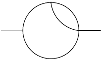
Differential renormalization can be applied not only to one-loop diagrams, but to multi-loop expressions. In general, new scales appear corresponding to the renormalization of the different subdiagrams that form the total expression. From the various types of subdivergences that can occur in a typical higher-loop diagram, we will take a closer look to one of them, where independent scales are neatly seen to appear at each stage: nested divergences. As an example we consider the following amplitude which, in principle, could form part of a bigger one: Δ⁡(x−y)​I1​(x−y)\Delta(x-y)I^{1}(x-y), where I1​(x)I^{1}(x) is

I1​(x−y)=∫d4​u​Δx​u​Δy​u2.I^{1}(x-y)=\int d^{4}u\Delta_{xu}\Delta^{2}_{yu}\;. (1.1.10)

It corresponds to a diagram that looks as follows
Refer to caption

Figure 1.1: Two-loop diagram with nested divergences.

As can be seen, divergences occur whenever 2 points come together. We can renormalize them starting from the most inner one, and proceeding recursively

[Δx​y​∫d4​u​Δx​u​[Δy​u2]R]R\displaystyle\left[\Delta_{xy}\int d^{4}u\Delta_{xu}[\Delta^{2}_{yu}]_{R}\right]_{R} =\displaystyle= [−14​(4​π2)41(x−y)2∫d4u1(x−u)2□ln⁡(y−u)2​M12(y−u)2]R\displaystyle\left[-\frac{1}{4(4\pi^{2})^{4}}\frac{1}{(x-y)^{2}}\int d^{4}u\;\frac{1}{(x-u)^{2}}\Box\frac{\ln(y-u)^{2}M^{2}_{1}}{(y-u)^{2}}\right]_{R} (1.1.11)
=\displaystyle= [14​(4​π2)3​ln⁡(x−y)2​M12(x−y)4]R\displaystyle\left[\frac{1}{4(4\pi^{2})^{3}}\frac{\ln(x-y)^{2}M_{1}^{2}}{(x-y)^{4}}\right]_{R}
=\displaystyle= −132​(4​π2)3​□​ln2⁡(x−y)2​M12+2​ln⁡(x−y)2​M22(x−y)2\displaystyle-\frac{1}{32(4\pi^{2})^{3}}\Box\frac{\ln^{2}(x-y)^{2}M_{1}^{2}+2\ln(x-y)^{2}M_{2}^{2}}{(x-y)^{2}}

where, in going to the second line, we have integrated by parts the d’alembertian and made use of □​1(x−u)2=δ⁡(x−u)\Box\frac{1}{(x-u)^{2}}=\delta(x-u). We observe the appearance of an independent scale associate with each renormalization step.

A systematic implementation of differential renormalization to all orders in perturbation theory was presented in [13]. The basics of the method are the separation of the divergences in two groups: one corresponds to divergences derived from two points collapsing, and the other to three or more points simultaneously closing up. For the first one the singularity is replaced with the renormalized form (once the derivatives are pulled in front), whereas the other one can be shown to be recursively written as two-point function problems of the first type. This procedure follows the BPHZ renormalization program and guarantees that differential renormalization maintains unitarity and it can be applied consistently (fulfilling locality and Lorentz invariance) to all orders [13].

1.1.2 Massive theories

Differential renormalization of massive theories has been studied in [7, 11]. The appearance of a bare mass does not interfere with the method, since DiffR is related to short-distance singularities and masses only change the long-distance behaviour of the correlators. Although in this work we will only deal with massless theories, we will give briefly as an example how this procedure works with massive λ​ϕ4\lambda\phi^{4}. The propagator of a particle of mass mm is

Δm​(x)\displaystyle\Delta_{m}(x) =\displaystyle= 14​π2​m2x2​K1​(m2​x2)\displaystyle\frac{1}{4\pi^{2}}\sqrt{\frac{m^{2}}{x^{2}}}K_{1}(\sqrt{m^{2}x^{2}}) (1.1.12)

where K1K_{1} is a modified Bessel function. Let us now consider again the 4-point function contribution; in this case is clear that the expression we have to renormalize is

[m2x2​K1​(m2​x2)]2.\displaystyle\left[\sqrt{\frac{m^{2}}{x^{2}}}K_{1}(\sqrt{m^{2}x^{2}})\right]^{2}\;. (1.1.13)

We have to solve the massive generalization of the differential equation (1.1.3), which has a solution of the form of

[m2x2​K1​(m2​x2)]R2\displaystyle\left[\sqrt{\frac{m^{2}}{x^{2}}}K_{1}(\sqrt{m^{2}x^{2}})\right]^{2}_{R} =\displaystyle= 12​(□−4​m2)​m2x2​K0​(m2​x2)​K1​(m2​x2)\displaystyle\frac{1}{2}(\Box-4m^{2})\sqrt{\frac{m^{2}}{x^{2}}}K_{0}(\sqrt{m^{2}x^{2}})K_{1}(\sqrt{m^{2}x^{2}}) (1.1.14)
+π2​ln⁡M¯2m2​δ​(x),\displaystyle+\pi^{2}\ln\frac{\bar{M}^{2}}{m^{2}}\delta(x)\;,

where M¯=2​M/γ\bar{M}=2M/\gamma and γ\gamma is the Euler constant. The general solution has a contact term which depends on a new mass parameter MM. This guarantees that in the limit where m→0m\rightarrow 0 the renormalized expressions for (1.1.4) and (1.1.14) coincide.

1.1.3 IR divergences

DiffR can be also applied to expression with IR divergences [15], i.e. expressions that exhibit a divergence for pμ→0p^{\mu}\rightarrow 0. The idea is to apply a dual version of Differential Renormalization to such quantities

[1p4]R~=−14            pln⁡p2/M¯I​R2p2+aI​Rδ(p).\left[\frac{1}{p^{4}}\right]_{\tilde{R}}=-\frac{1}{4}{\mathop{\mathchoice{\vbox{\vbox{\hrule height=0.4pt\hbox{\vrule width=0.4pt,height=6.0pt\kern 6.0pt\vrule width=0.4pt}\hrule height=0.4pt}}}{\vbox{\vbox{\hrule height=0.4pt\hbox{\vrule width=0.4pt,height=6.0pt\kern 6.0pt\vrule width=0.4pt}\hrule height=0.4pt}}}{\vbox{\vbox{\hrule height=0.4pt\hbox{\vrule width=0.4pt,height=3.75pt\kern 3.75pt\vrule width=0.4pt}\hrule height=0.4pt}}}{\vbox{\vbox{\hrule height=0.4pt\hbox{\vrule width=0.4pt,height=3.0pt\kern 3.0pt\vrule width=0.4pt}\hrule height=0.4pt}}}}\nolimits}_{p}\frac{\ln p^{2}/\bar{M}_{IR}^{2}}{p^{2}}+a_{IR}\delta(p)\;. (1.1.15)

We have defined for convenience M¯I​R=2​MI​R/γE\bar{M}_{IR}=2M_{IR}/\gamma_{E}, where γE\gamma_{E} is Euler’s constant, and distinguished the IR scale from the UV one. As DiffR is an implementation of Bogoliubov’s RR operation (an operation that yields directly renormalized correlation functions satisfying renormalization group equations), in momentum space this is an explicit realization of the so-called R~\tilde{R} operation that subtracts IR divergences. Again, diagrams with IR subdivergences are treated according to a recursion formula [16, 17] analogous to the UV one.
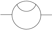
Refer to caption

Figure 1.2: Two-loop diagram with UV and IR divergences.

Now, when going to higher loops a new effect will show up, namely the coexistence of UV and IR scales. Let us start by examining a prototypical diagram where such divergences arise in a λ​ϕ3\lambda\phi^{3} type theory (figure 1.2). The associated amplitude that we have in this case is of the form G⁡(x−y)=Δ⁡(x−y)​I0​(x−y)G(x-y)=\Delta(x-y)I^{0}(x-y), where I0I^{0} is

I0​(x−y)\displaystyle I^{0}(x-y) =\displaystyle= ∫d4​u​d4​v​Δx​u​Δy​v​Δu​v2.\displaystyle\int d^{4}ud^{4}v\;\Delta_{xu}\Delta_{yv}\Delta^{2}_{uv}\;. (1.1.16)

We begin by renormalizing the inner UV divergence as

IR0​(x−y)\displaystyle I^{0}_{R}(x-y) =\displaystyle= −14​(4​π2)2∫d4ud4v□ln⁡(u−v)2​M2(u−v)2Δx​uΔv​y\displaystyle-\frac{1}{4(4\pi^{2})^{2}}\int d^{4}ud^{4}v\;\Box\frac{\ln(u-v)^{2}M^{2}}{(u-v)^{2}}\Delta_{xu}\Delta_{vy} (1.1.17)
=\displaystyle= 14​(4​π2)2​∫d4​u​ln⁡(u−y)2​M2(u−y)2​Δx​u.\displaystyle\frac{1}{4(4\pi^{2})^{2}}\int d^{4}u\;\frac{\ln(u-y)^{2}M^{2}}{(u-y)^{2}}\Delta_{xu}\;.

In order to renormalize the IR divergence we have to pass to momentum space

IR0​(x−y)\displaystyle I^{0}_{R}(x-y) =\displaystyle= −14​(4​π2)5∫d4ud4pd4qln⁡p2/M2p21q2e−i​p​(u−y)e−i​q​(x−u)\displaystyle-\frac{1}{4(4\pi^{2})^{5}}\int d^{4}ud^{4}pd^{4}q\;\frac{\ln p^{2}/M^{2}}{p^{2}}\frac{1}{q^{2}}e^{-ip(u-y)}e^{-iq(x-u)} (1.1.18)
=\displaystyle= −14​(4​π2)3∫d4pln⁡p2/M2p4e−i​p​(x−y).\displaystyle-\frac{1}{4(4\pi^{2})^{3}}\int d^{4}p\;\frac{\ln p^{2}/M^{2}}{p^{4}}e^{-ip(x-y)}\;.

We explicitly observe that the IR singularity at p→0p\rightarrow 0 involves an UV scale MM.

Since UV and IR overall divergences are local in coordinate and momentum space, respectively, the RR and R~\tilde{R} operations commute, and one can define an operation R∗=R~​RR^{*}=\tilde{R}R to renormalize both UV and IR divergences [16, 17]. The fact that the UV and IR renormalizations decouple means that the UV and IR renormalization scales should be independent. This is a non-trivial point that in DiffR can be achieved by a careful adjustment of the local terms involving both scales11 1 IR DiffR was investigated in [18] where it was concluded that the combination of UV and IR DiffR was inconsistent, as the results depended on the order in which integrations were performed. According to [19], however, this corresponds to the natural arbitrariness of the IR renormalization, and this author has actually proposed in [20] a consistent version of DiffR that deals with both UV and IR divergences. Our approach here will be closer to the original version of DiffR.

As we have to guarantee that the IR renormalization commute with a rescaling of MM, we have to fulfill the relation

M​δδ​M​[ln⁡p2/M¯2p4]R~=[M​δδ​M​ln⁡p2/M¯2p4]R~.M\frac{\delta}{\delta M}\left[\frac{\ln p^{2}/\bar{M}^{2}}{p^{4}}\right]_{\tilde{R}}=\left[M\frac{\delta}{\delta M}\frac{\ln p^{2}/\bar{M}^{2}}{p^{4}}\right]_{\tilde{R}}\;. (1.1.19)

If we consider the usual expression for the renormalization of (ln⁡p2/M¯2)/p4(\ln p^{2}/\bar{M}^{2})/p^{4}

[ln⁡p2/M¯2p4]R~=−18​□p​ln2⁡p2/M¯2+2​ln⁡p2/MI​R¯2p2,\displaystyle\left[\frac{\ln p^{2}/\bar{M}^{2}}{p^{4}}\right]_{\tilde{R}}=-\frac{1}{8}\Box_{p}\frac{\ln^{2}p^{2}/\bar{M}^{2}+2\ln p^{2}/\bar{M_{IR}}^{2}}{p^{2}}\;, (1.1.20)

we find that the left hand side of (1.1.19) is

M​δδ​M​[ln⁡p2/M¯2p4]R~\displaystyle M\frac{\delta}{\delta M}\left[\frac{\ln p^{2}/\bar{M}^{2}}{p^{4}}\right]_{\tilde{R}} =\displaystyle= 12​□p​ln⁡p2/M¯I​R2+ln⁡M¯2/M¯I​R2p2,\displaystyle\frac{1}{2}\Box_{p}\frac{\ln p^{2}/\bar{M}_{IR}^{2}+\ln{\bar{M}}^{2}/\bar{M}_{IR}^{2}}{p^{2}}\;, (1.1.21)

whereas the right and side has the form of

[M​δδ​M​ln⁡p2/M¯2p4]R~\displaystyle\left[M\frac{\delta}{\delta M}\frac{\ln p^{2}/\bar{M}^{2}}{p^{4}}\right]_{\tilde{R}} =\displaystyle= −2​[1p4]R\displaystyle-2\left[\frac{1}{p^{4}}\right]_{R} (1.1.22)
=\displaystyle= 12​□p​ln⁡p2/M¯I​R2p2,\displaystyle\frac{1}{2}\Box_{p}\frac{\ln p^{2}/\bar{M}_{IR}^{2}}{p^{2}}\;,

So, the second expression differs from the first one in a local term in momentum space, that will be a non local one in position space. Hence, in order to fulfill (1.1.19), we propose the following minimal solution that does the job [15]

[ln⁡p2/M¯2p4]R~=−18            p−ln2p2/M¯I​R2+2lnp2/M¯I​R2(1+lnp2/M¯2)p2+(aI​RlnMI​R2M2+bI​R)δ(p)\left[\frac{\ln p^{2}/\bar{M}^{2}}{p^{4}}\right]_{\tilde{R}}=-\frac{1}{8}{\mathop{\mathchoice{\vbox{\vbox{\hrule height=0.4pt\hbox{\vrule width=0.4pt,height=6.0pt\kern 6.0pt\vrule width=0.4pt}\hrule height=0.4pt}}}{\vbox{\vbox{\hrule height=0.4pt\hbox{\vrule width=0.4pt,height=6.0pt\kern 6.0pt\vrule width=0.4pt}\hrule height=0.4pt}}}{\vbox{\vbox{\hrule height=0.4pt\hbox{\vrule width=0.4pt,height=3.75pt\kern 3.75pt\vrule width=0.4pt}\hrule height=0.4pt}}}{\vbox{\vbox{\hrule height=0.4pt\hbox{\vrule width=0.4pt,height=3.0pt\kern 3.0pt\vrule width=0.4pt}\hrule height=0.4pt}}}}\nolimits}_{p}\frac{-\ln^{2}p^{2}/\bar{M}_{IR}^{2}+2\ln p^{2}/\bar{M}_{IR}^{2}\,(1+\ln p^{2}/\bar{M}^{2})}{p^{2}}+(a_{IR}\ln\frac{M^{2}_{IR}}{M^{2}}+b_{IR})\delta(p) (1.1.23)

This expression differs from the usual one by scale-dependent local terms proportional to ln2⁡M2/MI​R2\ln^{2}M^{2}/M_{IR}^{2} (apart from the explicit local terms with coefficients aI​Ra_{IR} and bI​Rb_{IR}). It should be used whenever the “new” scale is to be treated as independent from the “old” one, for consistency of the loop expansion. It has to be noted that when we consider a purely UV expression as in (1.1.11), we do not have to take care of all of this, because the extra term is cancelled in the RG equation when we derive wrt. the UV scales. With this, the result for I0I^{0} (not taking care of the local terms aI​Ra_{IR} and bI​Rb_{IR}) is

IR0​(x−y)\displaystyle I^{0}_{R}(x-y) =\displaystyle= 132​(4​π2)3​∫d4​p​□p​−ln2p2/M2I​R+2lnp2/M2I​R(1+lnp2/M2)p2​e−i​p​(x−y)\displaystyle\frac{1}{32(4\pi^{2})^{3}}\int d^{4}p\;\Box^{p}\frac{-\ln^{2}p^{2}/M^{2}_{IR}+2\ln p^{2}/M^{2}_{IR}\left(1+\ln p^{2}/M^{2}\right)}{p^{2}}e^{-ip(x-y)}
=\displaystyle= −(x−y)232​(4​π2)3∫d4p−ln2p2/M2I​R+2lnp2/M2I​R(1+lnp2/M2)p2e−i​p​(x−y),\displaystyle-\frac{(x-y)^{2}}{32(4\pi^{2})^{3}}\int d^{4}p\;\frac{-\ln^{2}p^{2}/M^{2}_{IR}+2\ln p^{2}/M^{2}_{IR}\left(1+\ln p^{2}/M^{2}\right)}{p^{2}}e^{-ip(x-y)}\;,

That in position space is

IR0​(x)\displaystyle I^{0}_{R}(x) =\displaystyle= 132​(4​π2)2​[ln2⁡x2​MI​R2+2​ln​x2​MI​R2​(1−ln⁡x2​M2)].\displaystyle\frac{1}{32(4\pi^{2})^{2}}\left[\ln^{2}x^{2}M^{2}_{IR}+2\ln x^{2}M^{2}_{IR}(1-\ln x^{2}M^{2})\right]\;. (1.1.25)

Observe that the UV scale MM only appears in (1.1.23), and hence in the above expression for I0I^{0}, in single logarithms. This is fine, for double logarithms of MM are expected to appear only when the bare expression contains both a UV subdivergence and a UV overall divergence. Finally, once we have obtained I0I^{0}, we can straightforwardly evaluate GG to be

G⁡(x)=132​(4​π2)3​ln2⁡x2​MI​R2+2​ln​x2​MI​R2​(1−ln⁡x2​M2)x2.\displaystyle G(x)=\frac{1}{32(4\pi^{2})^{3}}\frac{\ln^{2}x^{2}M^{2}_{IR}+2\ln x^{2}M^{2}_{IR}(1-\ln x^{2}M^{2})}{x^{2}}\;. (1.1.26)

1.1.4 Symmetries with DiffR

One of the important properties that is required to every sensible renormalization procedure is not to break gauge symmetry when it is applied to a gauge theory. For DiffR it is found that gauge symmetry is preserved as long as Ward identities can be always satisfied with the renormalized amplitudes (except anomalies). However, at the same time we find that we have to make always explicit use of these identities to fix all the ambiguities that have appeared in the calculations; in particular with Ward identities we relate the different scales that we have to use when renormalizing different amplitudes related by a symmetry(i.e. we fix a renormalization scheme).

As an example of this, consider the case of the one-loop renormalization of the photon self-energy in QED [14]. The bare expression is

Πμ​ν​(x)|b​a​r​e=−4​e2​[2​(∂μΔ⁡(x))​(∂νΔ⁡(x))−δμ​ν​(∂βΔ⁡(x))​(∂βΔ⁡(x))],\displaystyle\Pi_{\mu\nu}(x)|_{bare}=-4e^{2}\left[2(\partial_{\mu}\Delta(x))(\partial_{\nu}\Delta(x))-\delta_{\mu\nu}(\partial_{\beta}\Delta(x))(\partial_{\beta}\Delta(x))\right]\;, (1.1.27)

and renormalizing, this becomes

Πμ​ν​(x)|R\displaystyle\Pi_{\mu\nu}(x)|_{R} =\displaystyle= −e212​π4​[∂μ∂ν1x4−8​δμ​ν​1x6]R\displaystyle-\frac{e^{2}}{12\pi^{4}}\left[\partial_{\mu}\partial_{\nu}\frac{1}{x^{4}}-8\delta_{\mu\nu}\frac{1}{x^{6}}\right]_{R}
=\displaystyle= −e212​π4[−14∂μ∂ν□ln⁡x2​M12x2+14δμ​ν□□ln⁡x2​M22x2−8δμ​νμ2δ(x)].\displaystyle-\frac{e^{2}}{12\pi^{4}}\left[-\frac{1}{4}\partial_{\mu}\partial_{\nu}\Box\frac{\ln x^{2}M_{1}^{2}}{x^{2}}+\frac{1}{4}\delta_{\mu\nu}\Box\Box\frac{\ln x^{2}M^{2}_{2}}{x^{2}}-8\delta_{\mu\nu}\mu^{2}\delta(x)\right]\;.

In this expression we have renormalized with an independent scale the logarithmic divergence (M1M_{1}) and the quadratic one (M2M_{2}). At the same time, related to the latter, we have added a possible local term with a parameter of mass dimensions (μ\mu). The Ward identity satisfied by this expression imposes that this has to be transverse, so that we have to fix M1=M2M_{1}=M_{2} and μ2=0\mu^{2}=0.

When going to higher loop computations, the Ward identities play a non-trivial rôle, as they influence part of the divergences that are obtained in the next step. The reason is that these identities relate all the relevant mass scales found. So, they allow us to write the one-loop renormalized subdiagrams that made up the two-loop expressions in terms of the same scale, say MM, and fixed local terms, which then are promoted to logarithms of the scale. Going back to the example at two loops that was solved in (1.1.11), suppose that after imposing the Ward identities we have the inner divergence written as −14□lnx2M2/x2+aδ(x)-\frac{1}{4}\Box\ln x^{2}M^{2}/x^{2}+a\delta(x), with aa a fixed coefficient. Thus, in the two-loop expression we find

[Δx​y​∫d4​u​Δx​u​[Δy​u2]R]R\displaystyle\left[\Delta_{xy}\int d^{4}u\Delta_{xu}[\Delta^{2}_{yu}]_{R}\right]_{R} =\displaystyle= [14​(4​π2)4​ln⁡(y−u)2​M2+a(x−y)4]R\displaystyle\left[\frac{1}{4(4\pi^{2})^{4}}\frac{\ln(y-u)^{2}M^{2}+a}{(x-y)^{4}}\right]_{R}
=\displaystyle= −132​(4​π2)3​□​ln2x2M2+2lnx2M2′2+2alnx2M2′′2x2,\displaystyle-\frac{1}{32(4\pi^{2})^{3}}\Box\frac{\ln^{2}x^{2}M^{2}+2\ln x^{2}M_{2}^{\prime 2}+2a\ln x^{2}M_{2}^{\prime\prime 2}}{x^{2}}\;,

where M2′M_{2}^{\prime} and M2′′M_{2}^{\prime\prime} are two-loop scales. Hence, as we have anticipated, the one-loop Ward identities have fixed the coefficients of the logarithms of the scales in the two-loop final expression. Concerning the new two-loop scales M2′M_{2}^{\prime} and M2′′M_{2}^{\prime\prime}, it is clear that both can be set also equal to MM modulo a local ambiguity that will depend on quotients M2′/MM_{2}^{\prime}/M and M2′′/MM_{2}^{\prime\prime}/M (like in (1.1.6)). Again, use of the Ward identities would set these quotients to certain computable values. In other words, after use has been made of the symmetry, in the two-loop expression the only scale that remains can be chosen to be MM and sits only inside the terms with logarithms whose coefficients were determined from the one-loop Ward identities. This observation is at the heart of the present work an permeates implicitly all the calculations contained in it. So we repeat it here for full clarity: if one is interested in computing a physical amplitude at two loops, a concrete value of the local terms is essential and use Ward identities at two loops is unavoidable. If however, as is the case of the present work, one is looking for the RG equations, then all the relevant information on the scale MM resides in the terms with logarithms, whose coefficients only need one-loop Ward identities to be fixed.

1.2 Constrained Differential Renormalization

Constrained Differential Renormalization (CDR) was developed in [21, 22, 23, 27] to avoid the necessity of imposing Ward identities in each calculation to fix the renormalization scheme, as we have seen in the previous section. The idea is to give a procedure that allows us to fix the scheme a priory. Central to the fulfilment of the Ward identities (and the action principle, from which they can be derived) is that the application of the kinetic differential operator to some propagator line inside a Feynman graph is equivalent to the contraction of the line to a point [21]. This statement is guaranteed to hold if we apply the following set of rules

  1. 1.

    Differential reduction

    • •

      Functions with singular behaviour worse than logarithmic are reduced to derivatives of (at most) logarithmically divergent functions without introducing extra dimensionful constants.

    • •

      Logarithmically divergent expressions are written as derivatives of regular functions, introducing one single constant MM, which has dimensions of mass and plays the rôle of the renormalization group scale.

  2. 2.

    Formal integration by parts. We do not take care of the divergent surface terms that appear when we integrate by parts. Related to this, differentiation and renormalization must be two commutative operations: let FF an arbitrary function, then [∂F]R=∂[F]R[\partial F]_{R}=\partial[F]_{R}.

  3. 3.

    Renormalization rule of the delta function:

    [F⁡(x,x1,…,xn)​δ​(x−y)]R=[F⁡(x,x1,…,xn)]R​δ​(x−y)[F(x,x_{1},\ldots,x_{n})\delta(x-y)]_{R}=[F(x,x_{1},\ldots,x_{n})]_{R}\delta(x-y) (1.2.30)
  4. 4.

    Validity of the propagator equation

    [F⁡(x,x1,…,xn)​(□−m2)​Δm​(x)]R=−[F⁡(x,x1,…,xn)​δ​(x)]R[F(x,x_{1},\ldots,x_{n})(\Box-m^{2})\Delta_{m}(x)]_{R}=-[F(x,x_{1},\ldots,x_{n})\delta(x)]_{R} (1.2.31)

    where Δm\Delta_{m} is the propagator of a particle of mass mm and FF an arbitrary function.

The upshot is a basic set of renormalized expressions (basic functions) with different numbers of propagators and various differential operators acting only on one of them, involving a single scale MM. Therefore the CDR program amounts to the following two step operation:

  • •

    Express the Feynman diagram in terms of these basic functions performing all the index contractions (this is an important point, because CDR does not commute with index contraction) and, by means of the Leibniz rule, moving all the derivatives to make them act on one of the propagators.

  • •

    Replace the basic functions with their renormalized version.

Let us now obtain as an example some of these functions. Consider the one-point basic function Δ⁡(x)​δ​(x)\Delta(x)\delta(x) (this corresponds to the one-loop correction to the two-point function in λ​Φ4\lambda\Phi^{4} theory). Power counting and the locality of the expression implies that the most general renormalized value that we have for this is

[Δ⁡(x)​δ​(x)]R=(c​□+μ2)​δ​(x),\displaystyle[\Delta(x)\delta(x)]_{R}=(c\Box+\mu^{2})\delta(x)\;, (1.2.32)

where μ\mu is a mass-dimension constant and cc an adimensional constant. However, rule 11 implies that μ=0\mu=0. Now, considering [Δ⁡(x)​δ​(x)]R​δ​(y)[\Delta(x)\delta(x)]_{R}\delta(y) and using rule 33 we find

[Δ⁡(x)​δ​(x)]R​δ​(y)\displaystyle[\Delta(x)\delta(x)]_{R}\delta(y) =\displaystyle= [Δ⁡(x)​δ​(x)​δ​(x+y)]R=[Δ⁡(x)​δ​(x)]R​δ​(x+y)\displaystyle[\Delta(x)\delta(x)\delta(x+y)]_{R}=[\Delta(x)\delta(x)]_{R}\delta(x+y)

and integrating over xx we arrive to

δ⁡(y)​∫d4​x​[Δ⁡(x)​δ​(x)]R=[Δ⁡(y)​δ​(y)]R.\displaystyle\delta(y)\int d^{4}x\;[\Delta(x)\delta(x)]_{R}=[\Delta(y)\delta(y)]_{R}\;. (1.2.34)

Finally, with this result rule 22 implies that c=0c=0. Proceeding in a similar way we find that all the massless one-point functions in CDR vanish.

As two-point function examples, we will consider Δ​∂μΔ\Delta\partial_{\mu}\Delta and Δ​□​Δ\Delta\Box\Delta. In the first case we have to apply the Leibniz rule to find

[Δ⁡(x)​∂μΔ⁡(x)]R\displaystyle[\Delta(x)\partial_{\mu}\Delta(x)]_{R} =\displaystyle= ∂μ[Δ⁡(x)​Δ​(x)]R−[(∂μΔ⁡(x))​Δ​(x)]R\displaystyle\partial_{\mu}[\Delta(x)\Delta(x)]_{R}-[(\partial_{\mu}\Delta(x))\Delta(x)]_{R} (1.2.35)
=\displaystyle= 12∂μ[Δ2(x)]R=−18​(4​π2)2∂μ□ln⁡x2​M2x2,\displaystyle\frac{1}{2}\partial_{\mu}[\Delta^{2}(x)]_{R}=-\frac{1}{8(4\pi^{2})^{2}}\partial_{\mu}\Box\frac{\ln x^{2}M^{2}}{x^{2}}\;,

where we have used the result of (1.1.4). If we study now Δ​□​Δ\Delta\Box\Delta, we have only to use rule 4 to arrive at

[Δ⁡(x)​□​Δ​(x)]R\displaystyle[\Delta(x)\Box\Delta(x)]_{R} =\displaystyle= −[Δ⁡(x)​δ​(x)]R=0.\displaystyle-[\Delta(x)\delta(x)]_{R}=0\;. (1.2.36)

Here we present as a summary the most relevant CDR identities that are used in this work. We only list the massless examples, although a complete list including massive propagators can be found in [23, 27]

[Δ2]R​(x)\displaystyle\left[\Delta^{2}\right]_{R}(x) =\displaystyle= −14​(4​π2)2​□​ln⁡x2​M2x2\displaystyle-\frac{1}{4(4\pi^{2})^{2}}\Box\frac{\ln x^{2}M^{2}}{x^{2}}
[Δ​∂μΔ]R​(x)\displaystyle\left[\Delta\partial_{\mu}\Delta\right]_{R}(x) =\displaystyle= −18​(4​π2)2∂μ□ln⁡x2​M2x2\displaystyle-\frac{1}{8(4\pi^{2})^{2}}\partial_{\mu}\Box\frac{\ln x^{2}M^{2}}{x^{2}}
[Δ​∂μ∂νΔ]R​(x)\displaystyle\left[\Delta\partial_{\mu}\partial_{\nu}\Delta\right]_{R}(x) =\displaystyle= −112​(4​π2)2(∂μ∂ν−14δμ​ν□)□ln⁡x2​M2x2+\displaystyle-\frac{1}{12(4\pi^{2})^{2}}(\partial_{\mu}\partial_{\nu}-\frac{1}{4}\delta_{\mu\nu}\Box)\Box\frac{\ln x^{2}M^{2}}{x^{2}}+
+1288​π2(∂μ∂ν−δμ​ν□)δ(x)\displaystyle+\frac{1}{288\pi^{2}}(\partial_{\mu}\partial_{\nu}-\delta_{\mu\nu}\Box)\delta(x)
[Δ​□​Δ]R​(x)\displaystyle\left[\Delta\Box\Delta\right]_{R}(x) =\displaystyle= 0.\displaystyle 0\;. (1.2.37)

CDR can be applied to more than two propagators. In particular, when dealing with three propagators, defining T⁡[𝒪]=Δ​Δ​𝒪​ΔT[{\cal{O}}]=\Delta\Delta{\cal{O}}\Delta, we can find the following relation to hold when making a decomposition into trace and traceless parts [21, 23]

TR[∂μ∂ν]\displaystyle T^{R}[\partial_{\mu}\partial_{\nu}] =\displaystyle= TR[∂μ∂ν−14δμ​ν□]+14δμ​νTR[□]−1128​π2δμ​νδ(x)δ(y).\displaystyle T^{R}[\partial_{\mu}\partial_{\nu}-\frac{1}{4}\delta_{\mu\nu}\Box]+\frac{1}{4}\delta_{\mu\nu}T^{R}[\Box]-\frac{1}{128\pi^{2}}\delta_{\mu\nu}\delta(x)\delta(y)\;. (1.2.38)

When using other gauges different from Feynman gauge, some bare expressions are written in terms of a quantity we define as Δ¯​(x)=14​(4​π2)​ln⁡x2​s2\bar{\Delta}(x)=\frac{1}{4(4\pi^{2})}\ln x^{2}s^{2}, where ss is an irrelevant constant with mass dimension. For this structure, CDR prescribes [21]

[Δ​□​Δ¯]R​(x)\displaystyle\left[\Delta\Box\bar{\Delta}\right]_{R}(x) =\displaystyle= −14​(4​π2)2​□​ln⁡x2​M2x2\displaystyle-\frac{1}{4(4\pi^{2})^{2}}\Box\frac{\ln x^{2}M^{2}}{x^{2}}
[Δ​∂μ∂νΔ¯]R​(x)\displaystyle\left[\Delta\partial_{\mu}\partial_{\nu}\bar{\Delta}\right]_{R}(x) =\displaystyle= 14​(−δμ​ν​14​(4​π2)2​□​ln⁡x2​M2x2−132​π2​∂μ∂ν1x2).\displaystyle\frac{1}{4}\left(-\delta_{\mu\nu}\frac{1}{4(4\pi^{2})^{2}}\Box\frac{\ln x^{2}M^{2}}{x^{2}}-\frac{1}{32\pi^{2}}\partial_{\mu}\partial_{\nu}\frac{1}{x^{2}}\right)\;. (1.2.39)

CDR has been checked in abelian and non-abelian gauge theories [21, 24] and in supersymmetric calculations [25, 26]. As an example of its use, we will re-obtain the one-loop renormalization of the photon self-energy of QED that we have renormalized with DiffR in the previous section. From the bare expression (1.1.27) we apply rule number 2 to write it in terms of the CDR basic functions as

Πμ​ν​(x)|R\displaystyle\Pi_{\mu\nu}(x)|_{R} =\displaystyle= −4​e2​[2​∂μ(Δ​∂νΔ)−2​Δ​∂μ∂νΔ−δμ​ν​∂β(Δ​∂βΔ)+δμ​ν​(Δ​□​Δ)]R.\displaystyle-4e^{2}\left[2\partial_{\mu}(\Delta\partial_{\nu}\Delta)-2\Delta\partial_{\mu}\partial_{\nu}\Delta-\delta_{\mu\nu}\partial_{\beta}(\Delta\partial_{\beta}\Delta)+\delta_{\mu\nu}(\Delta\Box\Delta)\right]_{R}\;.

Now, we have to replace each basic expression with its renormalized value, and straightforwardly we arrive to

Πμ​ν​(x)|R\displaystyle\Pi_{\mu\nu}(x)|_{R} =\displaystyle= (∂μ∂ν−δμ​ν□)[e23​(4​π2)2□ln⁡x2​M2x2+e236​π2δ(x)].\displaystyle(\partial_{\mu}\partial_{\nu}-\delta_{\mu\nu}\Box)\left[\frac{e^{2}}{3(4\pi^{2})^{2}}\Box\frac{\ln x^{2}M^{2}}{x^{2}}+\frac{e^{2}}{36\pi^{2}}\delta(x)\right]\;. (1.2.41)

As we have remarked, CDR has fixed all the ambiguities a priori, obtaining a direct final result that is transverse, as it has to be to fulfill the Ward identity.

Finally, it is worth to mention that this method is equivalent to a momentum-space regularization method defined also in four dimensions: Constrained Implicit Regularization (CIR). Implicit Regularization [28, 29] is a regularization method based in the assumption of a regulating function as part of the integrand of divergent amplitudes, and the extension of the properties of regular integrals to regularized ones. As in differential renormalization, this procedure generates arbitrary parameters that with CIR are fixed a priori [30].

1.3 Two-loop uses of one-loop CDR results

As we have seen, one of the drawbacks of DiffR is the plethora of scales that pop up at each step of the calculation. In symmetric theories, at fixed order in the perturbative expansion, these scales should reduce to a single one upon use of the Ward identities. In the previous section we have explained how CDR paves the way to this reduction of scales at the one-loop level. So far, CDR has not been fully developed at loop-order higher than one, and therefore it is not useful for computing, say, scattering amplitudes. However, as is mentioned at the end of section 1.1.4, as long as we are interested in the RG equations, all that we need are the terms with logarithms, and to obtain them the knowledge of the local terms at one loop-level is enough. Hence, we will discuss both the way the logarithms are generated from one loop to the next, and the implementation of the CDR rules in such diagrams [31].

1.3.1 Nested divergences

This case is particularly simple because CDR can be applied in a systematic way. Starting from the “inner” divergence, its regularization according to CDR gives an expression with logarithms of a single scale (ln⁡x2​M2\ln x^{2}M^{2}) and fixed local terms. The one-loop Ward identities are fulfilled. In the next step, when tackling the outer part of the diagram, a simple logarithm like the one shown above is promoted to an expression of the form ln2⁡x2​M2+C​ln⁡x2​M′2\ln^{2}x^{2}M^{2}+C\ln x^{2}M^{\prime 2}, with CC a calculable coefficient and M′M^{\prime} a two-loop scale; at the same time, the local terms that multiply outer divergences will produce additional logarithms of new scales. CDR does not yet prescribe what the different two-loop scales should be; hence, we may take all of them the same, and equal to MM, at the price of leaving undetermined local terms which are irrelevant when obtaining the RG equation.

This simple scheme has some subtleties when considering diagrams with indices because, even at one-loop, index contraction does not commute with CDR. Therefore, the correct order is to first insert into the outer diagram the non-renormalized expression for the “inner” one-loop diagram, perform all the index contractions, and then renormalize. This crucial observations looks as the first one in a list of rules that eventually would setup the implementation of CDR at higher loops.

Let us consider now the two-loop example discussed in sections 1.1.1 and 1.1.4. If we had imposed CDR in the first step, M1=MM_{1}=M is the only scale generated upon renormalizing the most internal divergence, and the local one-loop ambiguity will be fixed to zero, as can be seen from (1.2.37). We express this by stating that the renormalization of I1​(x−y)=∫d4​u​Δx​u​Δy​u2I^{1}(x-y)=\int d^{4}u\Delta_{xu}\Delta^{2}_{yu} according to CDR rules is given by

IR1​(x)=14​(4​π2)2​ln⁡x2​M2x2.I^{1}_{R}(x)=\frac{1}{4(4\pi^{2})^{2}}\frac{\ln x^{2}M^{2}}{x^{2}}\;. (1.3.42)

Once we have this, to renormalize the complete two-loop expression Δ​I1\Delta I^{1}, we have to apply usual differential renormalization and set, modulo local terms, the two-loop mass-scale M2′=MM_{2}^{\prime}=M. So, we arrive to an expression of the form of

[Δ​I1]R​(x)=−132​(4​π2)3​□​ln2⁡x2​M2+2​ln⁡x2​M2x2+…,\displaystyle\left[\Delta I^{1}\right]_{R}(x)=-\frac{1}{32(4\pi^{2})^{3}}\Box\frac{\ln^{2}x^{2}M^{2}+2\ln x^{2}M^{2}}{x^{2}}+\ldots\;, (1.3.43)

where …\ldots stand for the two-loop local terms that we are not taking into account. Notice that in the rest of the work (unless explicitly stated otherwise) …\ldots in a two-loop renormalized expression like the one shown above will have the same meaning: local terms not considered. With this procedure we have renormalized all the different structures made of I1I^{1} that we have encountered in our calculations. Apart from the previous one, we have found the following relevant expressions

[Δ​∂μI1]R​(x)\displaystyle\left[\Delta\partial_{\mu}I^{1}\right]_{R}(x) =\displaystyle= −164​(4​π2)3∂μ□ln2⁡x2​M2+ln⁡x2​M2x2+…\displaystyle-\frac{1}{64(4\pi^{2})^{3}}\partial_{\mu}\Box\frac{\ln^{2}x^{2}M^{2}+\ln x^{2}M^{2}}{x^{2}}+\ldots (1.3.44)
[Δ​∂μ∂νI1]R​(x)\displaystyle\left[\Delta\partial_{\mu}\partial_{\nu}I^{1}\right]_{R}(x) =\displaystyle= −196​(4​π2)3[∂μ∂ν□ln2⁡x2​M2+23​ln⁡x2​M2x2\displaystyle-\frac{1}{96(4\pi^{2})^{3}}\left[\partial_{\mu}\partial_{\nu}\Box\frac{\ln^{2}x^{2}M^{2}+\frac{2}{3}\ln x^{2}M^{2}}{x^{2}}\right. (1.3.45)
−14δμ​ν□□ln2⁡x2​M2+113​ln⁡x2​M2x2]+…\displaystyle-\left.\frac{1}{4}\delta_{\mu\nu}\Box\Box\frac{\ln^{2}x^{2}M^{2}+\frac{11}{3}\ln x^{2}M^{2}}{x^{2}}\right]+\ldots
[Δ​□​I1]R​(x)\displaystyle\left[\Delta\Box I^{1}\right]_{R}(x) =\displaystyle= 132​(4​π2)2​□​□​ln⁡x2​M2x2+…\displaystyle\frac{1}{32(4\pi^{2})^{2}}\Box\Box\frac{\ln x^{2}M^{2}}{x^{2}}+\ldots (1.3.46)

To obtain each of these results, we only have to consider the CDR renormalization of I1I^{1}, and apply afterwards usual DiffR, setting all the two-loop mass scales equal to MM. Let us illustrate the simplicity of the procedure with Δ​∂μI1\Delta\partial_{\mu}I^{1}. Given the renormalized form of I1I^{1} we find

[Δ​∂μI1]R​(x)\displaystyle\left[\Delta\partial_{\mu}I^{1}\right]_{R}(x) =C​D​R\displaystyle\stackrel{{\scriptstyle CDR}}{{=}} 14​(4​π2)3​[1x2​∂μln⁡x2​M2x2]R\displaystyle\frac{1}{4(4\pi^{2})^{3}}\left[\frac{1}{x^{2}}\partial_{\mu}\frac{\ln x^{2}M^{2}}{x^{2}}\right]_{R} (1.3.47)
=D​i​f​f​R\displaystyle\stackrel{{\scriptstyle DiffR}}{{=}} −116​(4​π2)3​[∂μ1−2​ln⁡x2​M2x4]R\displaystyle-\frac{1}{16(4\pi^{2})^{3}}\left[\partial_{\mu}\frac{1-2\ln x^{2}M^{2}}{x^{4}}\right]_{R}
=\displaystyle= −164​(4​π2)3∂μ□ln2⁡x2​M2+ln⁡x2​M2x2+…\displaystyle-\frac{1}{64(4\pi^{2})^{3}}\partial_{\mu}\Box\frac{\ln^{2}x^{2}M^{2}+\ln x^{2}M^{2}}{x^{2}}+\ldots

1.3.2 Overlapping divergences

Diagrams with overlapping divergences are more complex as it is sometimes difficult to recognize the one-loop subdivergences that need to be treated with CDR to start with. Our approach will be to obtain through different methods (that we will explain later in detail), a list of renormalized two-loop integrals with overlapping divergences, where in each calculation one-loop CDR rules have been maintained in every step. Although this list is restricted to integrals with at most four derivatives acting on the propagators and two free indices, it is found to be very useful, as serves as a basis that we can use to express the renormalized overlapping contributions to two-point functions in theories with derivative couplings at two loops. As we detail in appendix B, these two-point functions are what we need to obtain the beta function if we use the background field method. This list will be applied in our work to renormalize and obtain the two-loop beta function of (Super)QED and (Super)Yang-Mills. We use the conventions of z=x−yz=x-y and ∂μ≡∂μx\partial_{\mu}\equiv\partial_{\mu}^{x}. We also define H⁡(x−y)≡H⁡(z)H(x-y)\equiv H(z) as

H⁡[𝒪1,𝒪2;𝒪3,𝒪4]=∫d4​u​d4​v​(𝒪1x​Δx​u)​(𝒪2x​Δx​v)​(𝒪3y​Δy​u)​(𝒪4y​Δy​v)​Δu​v,\displaystyle H[{\cal{O}}_{1},{\cal{O}}_{2}\;;\;{\cal{O}}_{3},{\cal{O}}_{4}]=\int d^{4}ud^{4}v\;({\cal{O}}_{1}^{x}\Delta_{xu})({\cal{O}}_{2}^{x}\Delta_{xv})({\cal{O}}_{3}^{y}\Delta_{yu})({\cal{O}}_{4}^{y}\Delta_{yv})\Delta_{uv}\;, (1.3.48)

with 𝒪i{\cal{O}}_{i} a differential operator.

HR​[1,1; 1,1]\displaystyle H^{R}[1,1\;;\;1,1] =\displaystyle= 6​π4​ξ​(3)(4​π2)4​Δ≡a​Δ\displaystyle\frac{6\pi^{4}\xi(3)}{(4\pi^{2})^{4}}\Delta\equiv a\Delta (1.3.49)
HR[∂μ,1; 1,1]\displaystyle H^{R}[\partial_{\mu},1\;;\;1,1] =\displaystyle= 3​ξ​(3)16​(4​π2)2​(∂μΔ)≡a2​∂μΔ\displaystyle\frac{3\xi(3)}{16(4\pi^{2})^{2}}(\partial_{\mu}\Delta)\equiv\frac{a}{2}\partial_{\mu}\Delta (1.3.50)
HR[1,∂λ; 1,∂λ]\displaystyle H^{R}[1,\partial_{\lambda}\;;\;1,\partial_{\lambda}] =\displaystyle= −116​(4​π2)3​□​ln⁡z2​M2z2+…\displaystyle-\frac{1}{16(4\pi^{2})^{3}}\Box\frac{\ln z^{2}M^{2}}{z^{2}}+\ldots (1.3.51)
∂λHR[1,∂μ; 1,∂λ]\displaystyle\partial_{\lambda}H^{R}[1,\partial_{\mu}\;;\;1,\partial_{\lambda}] =\displaystyle= −132​(4​π2)3∂μ□12​ln⁡z2​M2z2+…\displaystyle-\frac{1}{32(4\pi^{2})^{3}}\partial_{\mu}\Box\frac{\frac{1}{2}\ln z^{2}M^{2}}{z^{2}}+\dots (1.3.52)
∂λHR[1,1;∂λ∂ν,1]\displaystyle\partial_{\lambda}H^{R}[1,1\;;\;\partial_{\lambda}\partial_{\nu},1] =\displaystyle= 132​(4​π2)3​∂ν□​14​ln2​z2​M2+34​ln⁡z2​M2z2+…\displaystyle\frac{1}{32(4\pi^{2})^{3}}\partial_{\nu}\Box\frac{\frac{1}{4}\ln^{2}z^{2}M^{2}+\frac{3}{4}\ln z^{2}M^{2}}{z^{2}}+\ldots (1.3.53)
HR[1,∂λ;∂λ∂μ,1]\displaystyle H^{R}[1,\partial_{\lambda}\;;\;\partial_{\lambda}\partial_{\mu},1] =\displaystyle= 132​(4​π2)3​∂μ□​18​ln2​z2​M2−78​ln⁡z2​M2z2+…\displaystyle\frac{1}{32(4\pi^{2})^{3}}\partial_{\mu}\Box\frac{\frac{1}{8}\ln^{2}z^{2}M^{2}-\frac{7}{8}\ln z^{2}M^{2}}{z^{2}}+\ldots (1.3.54)
HR[∂μ∂λ,∂λ; 1,1]\displaystyle H^{R}[\partial_{\mu}\partial_{\lambda},\partial_{\lambda}\;;\;1,1] =\displaystyle= 132​(4​π2)3​∂μ□​−12​ln2​z2​M2−ln⁡z2​M2z2+…\displaystyle\frac{1}{32(4\pi^{2})^{3}}\partial_{\mu}\Box\frac{-\frac{1}{2}\ln^{2}z^{2}M^{2}-\ln z^{2}M^{2}}{z^{2}}+\ldots (1.3.55)
∂λHR[1,∂μ;∂ν∂λ,1]\displaystyle\partial_{\lambda}H^{R}[1,\partial_{\mu}\;;\;\partial_{\nu}\partial_{\lambda},1] =\displaystyle= 132​(4​π2)3[∂μ∂ν□18​ln2​z2​M2+18​ln⁡z2​M2z2\displaystyle\frac{1}{32(4\pi^{2})^{3}}\left[\partial_{\mu}\partial_{\nu}\Box\frac{\frac{1}{8}\ln^{2}z^{2}M^{2}+\frac{1}{8}\ln z^{2}M^{2}}{z^{2}}\right. (1.3.56)
+δμ​ν□□−14​ln⁡z2​M2z2]+…\displaystyle\left.+\delta_{\mu\nu}\Box\Box\frac{-\frac{1}{4}\ln z^{2}M^{2}}{z^{2}}\right]+\ldots
HR[1,∂μ; 1,∂ν]\displaystyle H^{R}[1,\partial_{\mu}\;;\;1,\partial_{\nu}] =\displaystyle= 132​(4​π2)3​δμ​ν​□​−12​ln⁡z2​M2z2+…\displaystyle\frac{1}{32(4\pi^{2})^{3}}\delta_{\mu\nu}\Box\frac{-\frac{1}{2}\ln z^{2}M^{2}}{z^{2}}+\ldots (1.3.57)
∂λHR[1,∂λ;∂μ∂ν,1]\displaystyle\partial_{\lambda}H^{R}[1,\partial_{\lambda}\;;\;\partial_{\mu}\partial_{\nu},1] =\displaystyle= 132​(4​π2)3[∂μ∂ν□−12​ln⁡z2​M2z2\displaystyle\frac{1}{32(4\pi^{2})^{3}}\left[\partial_{\mu}\partial_{\nu}\Box\frac{-\frac{1}{2}\ln z^{2}M^{2}}{z^{2}}\right. (1.3.58)
+δμ​ν□□18​ln2​z2​M2+38​ln⁡z2​M2z2]+…\displaystyle\left.+\delta_{\mu\nu}\Box\Box\frac{\frac{1}{8}\ln^{2}z^{2}M^{2}+\frac{3}{8}\ln z^{2}M^{2}}{z^{2}}\right]+\ldots
∂λHR[1,∂λ; 1,∂μ∂ν]\displaystyle\partial_{\lambda}H^{R}[1,\partial_{\lambda}\;;\;1,\partial_{\mu}\partial_{\nu}] =\displaystyle= 132​(4​π2)3[∂μ∂ν□12​ln⁡z2​M2z2\displaystyle\frac{1}{32(4\pi^{2})^{3}}\left[\partial_{\mu}\partial_{\nu}\Box\frac{\frac{1}{2}\ln z^{2}M^{2}}{z^{2}}\right. (1.3.59)
+δμ​ν□□18​ln2​z2​M2+38​ln⁡z2​M2z2]+…\displaystyle\left.+\delta_{\mu\nu}\Box\Box\frac{\frac{1}{8}\ln^{2}z^{2}M^{2}+\frac{3}{8}\ln z^{2}M^{2}}{z^{2}}\right]+\ldots
HR[1,1;∂μ∂ν,1]\displaystyle H^{R}[1,1\;;\;\partial_{\mu}\partial_{\nu},1] =\displaystyle= 132​(4​π2)3​δμ​ν​□​14​ln2​z2​M2+34​ln⁡z2​M2z2+…\displaystyle\frac{1}{32(4\pi^{2})^{3}}\delta_{\mu\nu}\Box\frac{\frac{1}{4}\ln^{2}z^{2}M^{2}+\frac{3}{4}\ln z^{2}M^{2}}{z^{2}}+\ldots (1.3.60)
∂λHR[1,1;∂λ∂ν,∂μ]\displaystyle\partial_{\lambda}H^{R}[1,1\;;\;\partial_{\lambda}\partial_{\nu},\partial_{\mu}] =\displaystyle= 132​(4​π2)3​δμ​ν​□​□​18​ln2​z2​M2+38​ln⁡z2​M2z2+…\displaystyle\frac{1}{32(4\pi^{2})^{3}}\delta_{\mu\nu}\Box\Box\frac{\frac{1}{8}\ln^{2}z^{2}M^{2}+\frac{3}{8}\ln z^{2}M^{2}}{z^{2}}+\ldots (1.3.61)
∂λHR[1,1;∂μ∂ν,∂λ]\displaystyle\partial_{\lambda}H^{R}[1,1\;;\;\partial_{\mu}\partial_{\nu},\partial_{\lambda}] =\displaystyle= 132​(4​π2)3​∂μ∂ν□​18​ln2​z2​M2+38​ln⁡z2​M2z2+…\displaystyle\frac{1}{32(4\pi^{2})^{3}}\partial_{\mu}\partial_{\nu}\Box\frac{\frac{1}{8}\ln^{2}z^{2}M^{2}+\frac{3}{8}\ln z^{2}M^{2}}{z^{2}}+\ldots (1.3.62)
HR[1,∂μ∂λ;∂ν∂λ,1]\displaystyle H^{R}[1,\partial_{\mu}\partial_{\lambda}\;;\;\partial_{\nu}\partial_{\lambda},1] =\displaystyle= 132​(4​π2)3[∂μ∂ν□16​ln2​z2​M2−536​ln⁡z2​M2z2\displaystyle\frac{1}{32(4\pi^{2})^{3}}\left[\partial_{\mu}\partial_{\nu}\Box\frac{\frac{1}{6}\ln^{2}z^{2}M^{2}-\frac{5}{36}\ln z^{2}M^{2}}{z^{2}}\right. (1.3.63)
+δμ​ν□□−124​ln2​z2​M2−2972​ln⁡z2​M2z2]+…\displaystyle\left.+\delta_{\mu\nu}\Box\Box\frac{-\frac{1}{24}\ln^{2}z^{2}M^{2}-\frac{29}{72}\ln z^{2}M^{2}}{z^{2}}\right]+\ldots
HR[1,∂μ∂λ; 1,∂ν∂λ]\displaystyle H^{R}[1,\partial_{\mu}\partial_{\lambda}\;;\;1,\partial_{\nu}\partial_{\lambda}] =\displaystyle= 132​(4​π2)3[∂μ∂ν□16​ln2​z2​M2+4936​ln⁡z2​M2z2\displaystyle\frac{1}{32(4\pi^{2})^{3}}\left[\partial_{\mu}\partial_{\nu}\Box\frac{\frac{1}{6}\ln^{2}z^{2}M^{2}+\frac{49}{36}\ln z^{2}M^{2}}{z^{2}}\right.
+δμ​ν□□−124​ln2​z2​M2−1172​ln⁡z2​M2z2]+…\displaystyle\left.+\delta_{\mu\nu}\Box\Box\frac{-\frac{1}{24}\ln^{2}z^{2}M^{2}-\frac{11}{72}\ln z^{2}M^{2}}{z^{2}}\right]+\ldots

These integrals are obtained basically applying two properties:

  • •

    Integral relations presented in appendix D. These exact relations allow us to put some of the integrals in terms of others that have an explicit d’alembertian acting on one of the propagators. Once we have done that, using □​Δ=−δ\Box\Delta=-\delta we can put these integrals in terms of the previously defined I1I^{1}. Then, we can straightforwardly apply the procedure for nested divergences that we have just presented in the previous section.22 2 Also this is the reason why we have not listed here the cases where the differential operator is a d’alembertian. For example, it is obvious that H⁡[□,1; 1,1]=−Δ​I1H[\Box,1\;;\;1,1]=-\Delta I^{1}.

  • •

    The decomposition into trace part, traceless part and fixed local term imposed by CDR to T[∂μ∂ν]T[\partial_{\mu}\partial_{\nu}] as (1.2.38).

As in the previous section, let us illustrate the procedure with an explicit example. Considering integral (1.3.53), this can be evaluated with both methods. First, we will make use of integral relation (D.1.2) and put this integral as sum of different integrals that have the divergences nested

∂λx∫\displaystyle\partial_{\lambda}^{x}\int d4​u​d4​v\displaystyle d^{4}ud^{4}v Δx​u​Δx​v​(∂λy∂νyΔy​u)​Δy​v​Δu​v=\displaystyle\Delta_{xu}\Delta_{xv}(\partial_{\lambda}^{y}\partial_{\nu}^{y}\Delta_{yu})\Delta_{yv}\Delta_{uv}=
=\displaystyle= −12∂νy∫d4ud4vΔx​uΔx​v(□Δy​u)Δy​vΔu​v\displaystyle-\frac{1}{2}\partial_{\nu}^{y}\int d^{4}ud^{4}v\;\Delta_{xu}\Delta_{xv}(\Box\Delta_{yu})\Delta_{yv}\Delta_{uv}
+∫d4ud4vΔx​uΔx​v(□Δy​u)(∂νyΔy​v)Δu​v\displaystyle+\int d^{4}ud^{4}v\;\Delta_{xu}\Delta_{xv}(\Box\Delta_{yu})(\partial_{\nu}^{y}\Delta_{yv})\Delta_{uv}
−12∂νy∂λy∫d4ud4vΔx​uΔx​v(∂λyΔy​u)Δy​vΔu​v.\displaystyle-\frac{1}{2}\partial_{\nu}^{y}\partial_{\lambda}^{y}\int d^{4}ud^{4}v\;\Delta_{xu}\Delta_{xv}(\partial_{\lambda}^{y}\Delta_{yu})\Delta_{yv}\Delta_{uv}\;.

Now, we have to apply as usual □​Δ=−δ\Box\Delta=-\delta and rewrite these integrals in terms of I1I^{1}. Note that the third integral can be easily shown to be finite, and its value is obtained in appendix D.1 to be a/4∂ν(□Δ)a/4\partial_{\nu}(\Box\Delta) with a=6​π4​ξ​(3)(4​π2)4a=\frac{6\pi^{4}\xi(3)}{(4\pi^{2})^{4}}) .

∂λx∫\displaystyle\partial_{\lambda}^{x}\int d4​u​d4​v\displaystyle d^{4}ud^{4}v Δx​u​Δx​v​(∂λy∂νyΔy​u)​Δy​v​Δu​v=\displaystyle\Delta_{xu}\Delta_{xv}(\partial_{\lambda}^{y}\partial_{\nu}^{y}\Delta_{yu})\Delta_{yv}\Delta_{uv}=
=\displaystyle= −12∂ν(ΔI1)+12(Δ∂νI1)+a4∂ν(□Δ).\displaystyle-\frac{1}{2}\partial_{\nu}(\Delta I^{1})+\frac{1}{2}(\Delta\partial_{\nu}I^{1})+\frac{a}{4}\partial_{\nu}(\Box\Delta)\;.

Applying the results found in section 1.3.1 for the I1I^{1} expression, the renormalized value of this is

∂λx∫\displaystyle\partial_{\lambda}^{x}\int d4​u​d4​v\displaystyle d^{4}ud^{4}v Δx​u​Δx​v​(∂λy∂νyΔy​u)​Δy​v​Δu​v=\displaystyle\Delta_{xu}\Delta_{xv}(\partial_{\lambda}^{y}\partial_{\nu}^{y}\Delta_{yu})\Delta_{yv}\Delta_{uv}= (1.3.67)
=\displaystyle= 132​(4​π2)3​∂ν□​14​ln2​z2​M2+34​ln⁡z2​M2z2+…\displaystyle\frac{1}{32(4\pi^{2})^{3}}\partial_{\nu}\Box\frac{\frac{1}{4}\ln^{2}z^{2}M^{2}+\frac{3}{4}\ln z^{2}M^{2}}{z^{2}}+\ldots

where …\ldots stands for the finite terms that we are not taking into account and z=x−yz=x-y.

We can also obtain this integral making use of the CDR relation (1.2.38) and perform a trace-traceless decomposition of (∂λy∂νyΔy​u)​Δy​v​Δu​v(\partial_{\lambda}^{y}\partial_{\nu}^{y}\Delta_{yu})\Delta_{yv}\Delta_{uv} as

∂λx∫\displaystyle\partial_{\lambda}^{x}\int d4​u​d4​v\displaystyle d^{4}ud^{4}v Δx​u​Δx​v​(∂λy∂νyΔy​u)​Δy​v​Δu​v=\displaystyle\Delta_{xu}\Delta_{xv}(\partial_{\lambda}^{y}\partial_{\nu}^{y}\Delta_{yu})\Delta_{yv}\Delta_{uv}= (1.3.68)
=\displaystyle= 14​∂νx∫d4​u​d4​v​Δx​u​Δx​v​(□​Δy​u)​Δy​v​Δu​v\displaystyle\frac{1}{4}\partial_{\nu}^{x}\int d^{4}ud^{4}v\;\Delta_{xu}\Delta_{xv}(\Box\Delta_{yu})\Delta_{yv}\Delta_{uv}
+∂λx∫d4ud4vΔx​uΔx​v[(∂λy∂νy−14δλ​ν□)Δy​u]Δy​vΔu​v\displaystyle+\partial_{\lambda}^{x}\int d^{4}ud^{4}v\;\Delta_{xu}\Delta_{xv}\left[(\partial_{\lambda}^{y}\partial_{\nu}^{y}-\frac{1}{4}\delta_{\lambda\nu}\Box)\Delta_{yu}\right]\Delta_{yv}\Delta_{uv}
−1128​π2∂νx∫d4ud4vΔx​uΔx​vδ(y−u)δ(y−v)\displaystyle-\frac{1}{128\pi^{2}}\partial_{\nu}^{x}\int d^{4}ud^{4}v\;\Delta_{xu}\Delta_{xv}\delta(y-u)\delta(y-v)
=\displaystyle= −14∂ν(ΔI1)R−1128​π2∂νΔR2+∂λIλ​ν​R\displaystyle-\frac{1}{4}\partial_{\nu}(\Delta I^{1})_{R}-\frac{1}{128\pi^{2}}\partial_{\nu}\Delta^{2}_{R}+\partial_{\lambda}I_{\lambda\nu\;R}
=\displaystyle= 132​(4​π2)3​∂ν□​14​ln2​z2​M2+34​ln⁡z2​M2z2+∂λIλ​ν​R,\displaystyle\frac{1}{32(4\pi^{2})^{3}}\partial_{\nu}\Box\frac{\frac{1}{4}\ln^{2}z^{2}M^{2}+\frac{3}{4}\ln z^{2}M^{2}}{z^{2}}+\partial_{\lambda}I_{\lambda\nu\;R}\;, (1.3.69)

where ∂λIλ​ν​R\partial_{\lambda}I_{\lambda\nu\;R} is the traceless part, that is finite. As we can see, both results agree. Although in this example we can perform the calculation with both methods with the same effort, with other integrals the situation is different, and we shall have to study each case in order to choose the best one. The explicit evaluation of all the integrals is presented in section D.1 of appendix D .

Chapter 2 Abelian QFT applications

In this chapter we apply the ideas and methods we have just presented to two of the most relevant examples of abelian gauge theories: QED and its supersymmetric extension, SuperQED. Although both theories have already been treated in [14, 37] using DiffR, we will show that our procedure simplifies the calculations, avoiding the use of Ward identities.

2.1 QED

QED is one of the simplest examples of a gauge theory, as the gauge symmetry group is an abelian one, U⁡(1)U(1). Hence, is a good theory to start with, as we can clearly see all the key points of our renormalization procedure.

2.1.1 The model

We use the same conventions as [14]. The d=4d=4 massless QED lagrangian is

ℒ\displaystyle{\cal{L}} =\displaystyle= 14Fμ​νFμ​ν+ψ¯γμ(∂μ+ieAμ)ψ,\displaystyle\frac{1}{4}F^{\mu\nu}F_{\mu\nu}+\bar{\psi}\gamma^{\mu}(\partial_{\mu}+ieA_{\mu})\psi\;, (2.1.1)

where ψ\psi is the fermion field, AμA_{\mu} is the U⁡(1)U(1) gauge field and Fμ​νF_{\mu\nu} is the field strength made up with AμA_{\mu} as Fμ​ν​(x)=∂μAν​(x)−∂νAμ​(x)F_{\mu\nu}(x)=\partial_{\mu}A_{\nu}(x)-\partial_{\nu}A_{\mu}(x). The γ\gamma matrices satisfy the Clifford algebra {γμ,γν}=2​δμ​ν\left\{\gamma_{\mu}\,,\,\gamma_{\nu}\right\}=2\delta_{\mu\nu}.

With ww an infinitesimal parameter, the QED action is invariant under the following U⁡(1)U(1) transformations

Aμ→Aμ−1e​∂μw\displaystyle A_{\mu}\rightarrow A_{\mu}-\frac{1}{e}\partial_{\mu}w
ψ→ψ+i​ψ​w\displaystyle\psi\rightarrow\psi+i\psi w
ψ¯→ψ¯−i​ψ¯​w.\displaystyle\bar{\psi}\rightarrow\bar{\psi}-i\bar{\psi}w\;. (2.1.2)

Hence, when quantizing QED we have to take care of this invariance. We have an infinite number of different gauge field configurations (those obtained through gauge transformations from a given one) that correspond to the same physical state. In a path integral approach, we want to integrate only over the relevant gauge field configurations; hence, we have to pick up only one field from each gauge orbit. To accomplish this there is a well-known procedure [32, 47] which implies that we have to add to the action a gauge fixing term that depends on a new parameter α\alpha and possible auxiliary fields (Faddeev-Popov ghosts fields, that in the concrete case of QED and SuperQED are not relevant). Different values for α\alpha correspond to different gauge choices. In particular, in our calculation we will use α=1\alpha=1 (Feynman gauge). The complete lagrangian is then

ℒ\displaystyle{\cal{L}} =\displaystyle= 14Fμ​νFμ​ν+12​α(∂μAμ)2+ψ¯γμ(∂μ+ieAμ)ψ.\displaystyle\frac{1}{4}F^{\mu\nu}F_{\mu\nu}+\frac{1}{2\alpha}(\partial_{\mu}A_{\mu})^{2}+\bar{\psi}\gamma^{\mu}(\partial_{\mu}+ieA_{\mu})\psi\;. (2.1.3)

With this action the gauge field and fermion propagators (in a generic gauge) are

Δμ​ν​(x−y)\displaystyle\Delta_{\mu\nu}(x-y) =\displaystyle= 116​π2(δμ​ν□+(α−1)∂μ∂ν)ln(x−y)2s2\displaystyle\frac{1}{16\pi^{2}}\left(\delta_{\mu\nu}\Box+(\alpha-1)\partial_{\mu}\partial_{\nu}\right)\ln(x-y)^{2}s^{2}
S⁡(x−y)\displaystyle S(x-y) =\displaystyle= −γλ∂λΔ(x−y),\displaystyle-\gamma^{\lambda}\partial_{\lambda}\Delta(x-y)\;, (2.1.4)

where ss stands for an irrelevant constant with mass dimension. Also, considering the expansion of the effective action, we write the terms corresponding to the vacuum polarization Πμ​ν\Pi_{\mu\nu} and fermion self-energy Σ\Sigma as

Γe​f​f\displaystyle\Gamma_{eff} =\displaystyle= 12∫d4xd4yAμ(x)[((1−1α)∂μ∂ν−δμ​ν□)δ(4)(x−y)−Πμ​ν(x−y)]Aν(y)\displaystyle\frac{1}{2}\int d^{4}xd^{4}y\;A_{\mu}(x)\left[\left(\left(1-\frac{1}{\alpha}\right)\partial_{\mu}\partial_{\nu}-\delta_{\mu\nu}\Box\right)\delta^{(4)}(x-y)-\Pi_{\mu\nu}(x-y)\right]A_{\nu}(y) (2.1.5)
+∫d4xd4yψ¯(x)(γμ∂μδ(4)(x−y)−Σ(x−y))ψ(y)+…\displaystyle+\int d^{4}xd^{4}y\;\bar{\psi}(x)(\gamma^{\mu}\partial_{\mu}\delta^{(4)}(x-y)-\Sigma(x-y))\psi(y)+\ldots
Background field method

Fixing the gauge is necessary in order to quantize the theory, but has the drawback to make us lose explicit gauge invariance in the intermediate results. In order to avoid this, the background field method was developed [4]. As the method is detailed in appendix B, we only briefly outline it here. The key point is the splitting of the gauge field in two parts: the quantum and the background fields (AμA_{\mu} and BμB_{\mu} respectively)

Aμ→Aμ+Bμ.\displaystyle A_{\mu}\rightarrow A_{\mu}+B_{\mu}\;. (2.1.6)

We can use AμA_{\mu} as the integration variable of the partition function, which implies that the gauge has to be fixed only for this field. As a result, we retain explicit gauge invariance in BμB_{\mu}. Along with this, as is shown in appendix B, this procedure has other relevant consequences: the coupling constant and the background field renormalizations are related, which implies that the beta function can be obtained only from the two-point function contribution. Hence, we have a background effective action of the form

Γe​f​f​[B]\displaystyle\Gamma_{eff}[B] =\displaystyle= 12∫d4xd4yBμ(x)[(∂μ∂ν−δμ​ν□)δ(4)(x−y)−Πμ​νB​B(x−y)]Bν(y)+…,\displaystyle\frac{1}{2}\int d^{4}xd^{4}y\;B_{\mu}(x)\left[\left(\partial_{\mu}\partial_{\nu}-\delta_{\mu\nu}\Box\right)\delta^{(4)}(x-y)-\Pi^{BB}_{\mu\nu}(x-y)\right]B_{\nu}(y)+\ldots\;,

and our aim is to calculate the two-loop expansion of the two-point 1PI function Πμ​νB​B\Pi^{BB}_{\mu\nu}. Notice also that, as the infinitesimal gauge transformation of the unsplit theory does not depend on the quantum gauge field, we can choose in the split theory the usual gauge fixing condition G=∂μAμG=\partial^{\mu}A_{\mu}. So, we have a split lagrangian of the form of

ℒ\displaystyle{\cal{L}} =\displaystyle= 14Fμ​νFμ​ν+14Bμ​νBμ​ν+12​α(∂μAμ)2+ψ¯γμ(∂μ+ieAμ)ψ+ieψ¯γμBμψ,\displaystyle\frac{1}{4}F^{\mu\nu}F_{\mu\nu}+\frac{1}{4}B^{\mu\nu}B_{\mu\nu}+\frac{1}{2\alpha}(\partial_{\mu}A_{\mu})^{2}+\bar{\psi}\gamma^{\mu}(\partial_{\mu}+ieA_{\mu})\psi+ie\bar{\psi}\gamma^{\mu}B_{\mu}\psi\;, (2.1.8)

with Bμ​ν=∂μBν−∂νBμB_{\mu\nu}=\partial_{\mu}B_{\nu}-\partial_{\nu}B_{\mu}. From this lagrangian, we have two relevant interaction vertices, which are shown in figure 2.1.

Refer to caption

Figure 2.1: QED interaction vertices. Thick wavy lines represent background external fields and thin wavy lines correspond to quantum gauge field propagators. Solid lines represent fermion fields.

2.1.2 One-loop level

Refer to caption

Figure 2.2: One-loop QED diagrams.

We first consider the one-loop renormalization of the background photon and fermion self-energies. The diagrams that correspond to these contributions are those of figure 2.2, where thick lines represent BμB_{\mu} fields, and thin ones correspond to AμA_{\mu}. The correction to the background self-energy is what we need to obtain the one-loop coefficient of the beta function, although it will not be used in two-loop calculations. On the other hand, the fermion self-energy will be not relevant for the one-loop beta function study, but it will be used afterwards as a one-loop insertion in a two-loop diagram.

Photon self-energy

We consider now the one-loop contribution to the photon self-energy Πμ​ν\Pi_{\mu\nu}. The expression for this diagram is

Πμ​ν​(1)B​B​(x−y)\displaystyle\Pi_{\mu\nu\;(1)}^{BB}(x-y) =\displaystyle= −(i​e)2​T​r​[γμ​γλ​∂λxΔ​γν​γσ​∂σyΔ]\displaystyle-(ie)^{2}Tr\left[\gamma_{\mu}\gamma^{\lambda}\partial_{\lambda}^{x}\Delta\gamma_{\nu}\gamma^{\sigma}\partial_{\sigma}^{y}\Delta\right] (2.1.9)
=\displaystyle= −e2​T​r​[γμ​γλ​γν​γσ]​(∂λ(Δ​∂σΔ)−Δ​∂λ∂σΔ).\displaystyle-e^{2}Tr\left[\gamma_{\mu}\gamma^{\lambda}\gamma_{\nu}\gamma^{\sigma}\right]\left(\partial_{\lambda}(\Delta\partial_{\sigma}\Delta)-\Delta\partial_{\lambda}\partial_{\sigma}\Delta\right)\;.

To proceed with the CDR program, we first have to perform all the index contractions, writing this diagram in terms of the basic CDR functions (1.2.37). To do that, we have to apply in 2.1.9 the following Clifford algebra result

T​r​[γμ​γλ​γν​γσ]=4​(δμ​λ​δν​σ−δμ​ν​δλ​σ+δμ​σ​δν​λ).\displaystyle Tr\left[\gamma_{\mu}\gamma_{\lambda}\gamma_{\nu}\gamma_{\sigma}\right]=4(\delta_{\mu\lambda}\delta_{\nu\sigma}-\delta_{\mu\nu}\delta_{\lambda\sigma}+\delta_{\mu\sigma}\delta_{\nu\lambda})\;. (2.1.10)

which allows us to find the fully expanded expression as

Πμ​ν​(1)B​B​(x)\displaystyle\Pi_{\mu\nu\;(1)}^{BB}(x) =\displaystyle= −4​e2​[2​∂μ(Δ​∂νΔ)−2​Δ​∂μ∂νΔ−δμ​ν​∂λ(Δ​∂λΔ)−δμ​ν​Δ​□​Δ].\displaystyle-4e^{2}\left[2\partial_{\mu}(\Delta\partial_{\nu}\Delta)-2\Delta\partial_{\mu}\partial_{\nu}\Delta-\delta_{\mu\nu}\partial_{\lambda}(\Delta\partial_{\lambda}\Delta)-\delta_{\mu\nu}\Delta\Box\Delta\right]\;. (2.1.11)

Now, CDR renormalization of this expression entails only to replace these basic functions with their renormalized values. The full one-loop renormalized background self-energy is given by [14, 21]

Πμ​ν​(1)B​B​(x)|R\displaystyle\left.\Pi_{\mu\nu\;(1)}^{BB}(x)\right|_{R} =\displaystyle= −(∂μ∂ν−δμ​ν□)[−e212​π2​(4​π2)□ln⁡x2​M2x2−e236​π2δ(x)].\displaystyle-(\partial_{\mu}\partial_{\nu}-\delta_{\mu\nu}\Box)\left[-\frac{e^{2}}{12\pi^{2}(4\pi^{2})}\Box\frac{\ln x^{2}M^{2}}{x^{2}}-\frac{e^{2}}{36\pi^{2}}\delta(x)\right]\;. (2.1.12)

As was guaranteed by the use of CDR, this result is transverse (as is required by the Ward identities), and has the ambiguity (local term) fixed.

Fermion self-energy

We will also consider the renormalization of the fermion self-energy Σ\Sigma. In a general gauge, the bare expression for this diagram is

Σ(1)​(x)\displaystyle\Sigma_{(1)}(x) =\displaystyle= e2​γμ​Δμ​ν​(x)​γλ​∂λΔ⁡(x)​γν.\displaystyle e^{2}\gamma_{\mu}\Delta_{\mu\nu}(x)\gamma^{\lambda}\partial_{\lambda}\Delta(x)\gamma_{\nu}\;. (2.1.13)

By making use of the expression for the photon propagator in a generic gauge (2.1.4), we can replace the basic functions by their CDR values and obtain the renormalized fermion self-energy as [14, 21]

Σ(1)​(x)|R\displaystyle\left.\Sigma_{(1)}(x)\right|_{R} =\displaystyle= e2​γλ​[14​(4​π2)2​∂λ□​ln⁡x2​M2x2+(α−1)​(14​(4​π2)2​∂λ□​ln⁡x2​M2x2+116​π2​∂λδ⁡(x))].\displaystyle e^{2}\gamma^{\lambda}\left[\frac{1}{4(4\pi^{2})^{2}}\partial_{\lambda}\Box\frac{\ln x^{2}M^{2}}{x^{2}}+(\alpha-1)\left(\frac{1}{4(4\pi^{2})^{2}}\partial_{\lambda}\Box\frac{\ln x^{2}M^{2}}{x^{2}}+\frac{1}{16\pi^{2}}\partial_{\lambda}\delta(x)\right)\right].

2.1.3 Two-loop level

Refer to caption

Figure 2.3: Two-loop QED diagrams.

Now we proceed with the two-loop case. There are two relevant graphs with external background fields. Diagram (a) has the divergences nested, whereas diagram (b) has overlapping divergences.

Diagram (a)

The expression for this diagram is

Πμ​ν​(2​a)B​B​(x−y)\displaystyle\Pi^{BB}_{\mu\nu\;(2\;a)}(x-y) =\displaystyle= −(ie)2∫d4ud4vTr[γμγλ(−∂λxΔx​u)Σ(1)(u−v)γε(−∂εvΔv​y)γνγσ\displaystyle-(ie)^{2}\int d^{4}ud^{4}v\;Tr\left[\gamma_{\mu}\gamma^{\lambda}(-\partial_{\lambda}^{x}\Delta_{xu})\Sigma^{(1)}(u-v)\gamma^{\varepsilon}(-\partial_{\varepsilon}^{v}\Delta_{vy})\gamma_{\nu}\gamma^{\sigma}\right. (2.1.15)
×(−∂σyΔy​x)].\displaystyle\left.\times(-\partial_{\sigma}^{y}\Delta_{yx})\right].

where Σ(1)\Sigma^{(1)} is the one-loop fermion self-energy. In the following we will restrict ourselves to Feynman gauge, as the term that takes care of the running of the gauge parameter in the RG equation will be shown not to be relevant for the two-loop beta function [14]. We will discuss this later in detail, when we apply the RG equation. So, in this gauge, the bare fermion self-energy is

Σ(1)​(x)\displaystyle\Sigma_{(1)}(x) =\displaystyle= −2​e2​γλ​[Δ​∂λΔ]​(x).\displaystyle-2e^{2}\gamma^{\lambda}\left[\Delta\partial_{\lambda}\Delta\right](x)\;. (2.1.16)

As we stated in section 1.2, CDR imposes a strict order to the operations of index contraction and renormalization: first all the indices should be contracted, and only after that we can renormalize. Inserting here the bare fermion self-energy we are keeping this order.

Expanding the expression of Πμ​ν​(2​a)B​B\Pi^{BB}_{\mu\nu\;(2\;a)} we find

Πμ​ν​(2​a)B​B​(x−y)\displaystyle\Pi^{BB}_{\mu\nu\;(2\;a)}(x-y) =\displaystyle= −2e4Tr[γμγλγργεγνγσ](∂σxΔx​y)∂λx∂εx∫d4ud4vΔx​uΔy​v(Δu​v∂ρuΔu​v).\displaystyle-2e^{4}Tr[\gamma_{\mu}\gamma_{\lambda}\gamma_{\rho}\gamma_{\varepsilon}\gamma_{\nu}\gamma_{\sigma}](\partial_{\sigma}^{x}\Delta_{xy})\partial_{\lambda}^{x}\partial_{\varepsilon}^{x}\int d^{4}ud^{4}v\;\Delta_{xu}\Delta_{yv}(\Delta_{uv}\partial^{u}_{\rho}\Delta_{uv})\;.

In order to simplify the notation, we define an integral expression of the form

Iμ0​(x−y)=∫d4​u​d4​v​Δx​u​Δy​v​(Δu​v​∂μΔu​v).I^{0}_{\mu}(x-y)=\int d^{4}ud^{4}v\;\Delta_{xu}\Delta_{yv}(\Delta_{uv}\partial_{\mu}\Delta_{uv})\;. (2.1.18)

Then, with standard Clifford algebra, we can write () as

Πμ​ν​(2​a)B​B​(x)\displaystyle\Pi^{BB}_{\mu\nu\;(2\;a)}(x) =\displaystyle= e4[−32(∂μΔ)∂λ∂νIλ0+16δμ​ν(∂σΔ)∂λ∂σIλ0+16(∂μΔ)□Iν0−8δμ​ν(∂ρΔ)□Iρ0].\displaystyle e^{4}\left[-32(\partial_{\mu}\Delta)\partial_{\lambda}\partial_{\nu}I^{0}_{\lambda}+16\delta_{\mu\nu}(\partial_{\sigma}\Delta)\partial_{\lambda}\partial_{\sigma}I^{0}_{\lambda}+16(\partial_{\mu}\Delta)\Box I^{0}_{\nu}-8\delta_{\mu\nu}(\partial_{\rho}\Delta)\Box I^{0}_{\rho}\right]\;.

The renormalization of Iμ0I^{0}_{\mu} is studied in section D.2.2 of appendix D. It is found there that this integral expression verifies ∂μIμ​R0=−12​IR1\partial^{\mu}I^{0}_{\mu\;R}=-\frac{1}{2}I^{1}_{R} and □I0μ​R=−12∂μI1R\Box I^{0}_{\mu\;R}=-\frac{1}{2}\partial_{\mu}I^{1}_{R}. Thus, we need only the renormalized value that we have previously obtained for I1I^{1}. We have finally

Πμ​ν​(2​a)B​B​(x)|R\displaystyle\left.\Pi^{BB}_{\mu\nu\;(2\;a)}(x)\right|_{R} =\displaystyle= e424​(4​π2)3​[∂μ∂ν−ln2⁡x2​M2−53​ln⁡x2​M2x2+δμ​ν​□​□​ln2⁡x2​M2+83​ln⁡x2​M2x2]\displaystyle\frac{e^{4}}{24(4\pi^{2})^{3}}\left[\partial_{\mu}\partial_{\nu}\frac{-\ln^{2}x^{2}M^{2}-\frac{5}{3}\ln x^{2}M^{2}}{x^{2}}+\delta_{\mu\nu}\Box\Box\frac{\ln^{2}x^{2}M^{2}+\frac{8}{3}\ln x^{2}M^{2}}{x^{2}}\right]
+…\displaystyle+\ldots
Diagram (b)

This diagram, opposite to the previous one, has overlapping divergences. Following the procedure presented in section 1.3.2, we will express this in terms of the integrals listed in that section. We begin by considering the bare contribution

Πμ​ν​(2​b)B​B​(x−y)\displaystyle\Pi_{\mu\nu\;(2\;b)}^{BB}(x-y) =\displaystyle= −(ie)4∫d4ud4vTr[γμ(γα∂αxΔx​u)γρ(γβ∂βuΔu​y)γν\displaystyle-(ie)^{4}\int d^{4}ud^{4}v\;Tr\left[\gamma_{\mu}(\gamma^{\alpha}\partial^{x}_{\alpha}\Delta_{xu})\gamma^{\rho}(\gamma^{\beta}\partial_{\beta}^{u}\Delta_{uy})\gamma_{\nu}\right.
×(γλ∂λyΔy​v)γρ(γσ∂σΔv​x)Δu​v],\displaystyle\times\left.(\gamma^{\lambda}\partial_{\lambda}^{y}\Delta_{yv})\gamma_{\rho}(\gamma^{\sigma}\partial_{\sigma}\Delta_{vx})\Delta_{uv}\right]\;,

or, written in terms of the expressions we defined as HH in (1.3.48)

Πμ​ν​(2​b)B​B​(x−y)\displaystyle\Pi_{\mu\nu\;(2\;b)}^{BB}(x-y) =\displaystyle= 2e4Tr[γμγαγργβγνγλγργσ]H[∂α,∂σ;∂β,∂λ].\displaystyle 2e^{4}Tr[\gamma_{\mu}\gamma_{\alpha}\gamma^{\rho}\gamma_{\beta}\gamma_{\nu}\gamma_{\lambda}\gamma_{\rho}\gamma_{\sigma}]H[\partial_{\alpha},\partial_{\sigma}\;;\;\partial_{\beta},\partial_{\lambda}]\;.

If we use the identity for γ\gamma matrices γμ​γν​γρ​γσ​γμ=−2​γσ​γρ​γν\gamma^{\mu}\gamma_{\nu}\gamma_{\rho}\gamma_{\sigma}\gamma_{\mu}=-2\gamma_{\sigma}\gamma_{\rho}\gamma_{\nu} [47] and integrate by parts the derivatives acting over Δx​u\Delta_{xu} and Δy​v\Delta_{yv}, we find that this diagram can be put as

Πμ​νB​B​(2​b)​(x−y)\displaystyle\Pi_{\mu\nu}^{BB\;(2\;b)}(x-y) =\displaystyle= 2e4Tr[γμγαγλγνγβγσ](−∂αx∂λxH[1,∂σ;∂βx,1]−∂αxH[1,∂σ;∂β∂λ,1]\displaystyle 2e^{4}Tr[\gamma_{\mu}\gamma_{\alpha}\gamma_{\lambda}\gamma_{\nu}\gamma_{\beta}\gamma_{\sigma}]\left(-\partial_{\alpha}^{x}\partial_{\lambda}^{x}H[1,\partial_{\sigma}\;;\;\partial^{x}_{\beta},1]-\partial^{x}_{\alpha}H[1,\partial_{\sigma}\;;\;\partial_{\beta}\partial_{\lambda},1]\right. (2.1.23)
+∂λxH[1,∂α∂σ;∂β,1]+H[1,∂α∂σ;∂β∂λ,1]).\displaystyle\left.+\partial^{x}_{\lambda}H[1,\partial_{\alpha}\partial_{\sigma}\;;\;\partial_{\beta},1]+H[1,\partial_{\alpha}\partial_{\sigma}\;;\;\partial_{\beta}\partial_{\lambda},1]\right)\;.

Using the properties of the trace, the clifford algebra definition {γμ,γν}=2​δμ​ν\left\{\gamma_{\mu}\,,\,\gamma_{\nu}\right\}=2\delta_{\mu\nu} and usual γ\gamma matrices results as T​r​[γμ​γλ​γν​γβ]=4​(δμ​λ​δν​β−δμ​ν​δλ​β+δμ​β​δν​λ)Tr[\gamma_{\mu}\gamma_{\lambda}\gamma_{\nu}\gamma_{\beta}]=4(\delta_{\mu\lambda}\delta_{\nu\beta}-\delta_{\mu\nu}\delta_{\lambda\beta}+\delta_{\mu\beta}\delta_{\nu\lambda}), we can write the right hand-side of the previous equation as

e4\displaystyle e^{4} [\displaystyle\left[\right. −8δμ​ν□H[1,∂λ;∂λ,1]+16∂μxH[1,∂ν;□,1]−8δμ​ν∂λxH[1,∂λ;□,1]\displaystyle-8\delta_{\mu\nu}\Box H[1,\partial_{\lambda}\;;\;\partial_{\lambda},1]+16\partial_{\mu}^{x}H[1,\partial_{\nu}\;;\;\Box,1]-8\delta_{\mu\nu}\partial_{\lambda}^{x}H[1,\partial_{\lambda}\;;\;\Box,1]
−16∂μxH[1,∂λ;∂λ∂ν,1]+16∂λxH[1,∂λ;∂μ∂ν,1]−16∂λxH[1,∂μ;∂λ∂ν,1]\displaystyle-16\partial_{\mu}^{x}H[1,\partial_{\lambda}\;;\;\partial_{\lambda}\partial_{\nu},1]+16\partial_{\lambda}^{x}H[1,\partial_{\lambda}\;;\;\partial_{\mu}\partial_{\nu},1]-16\partial_{\lambda}^{x}H[1,\partial_{\mu}\;;\;\partial_{\lambda}\partial_{\nu},1]
−16∂μH[1,□;∂ν,1]+8δμ​ν∂λxH[1,□;∂λ,1]+16∂λxH[1,∂λ∂μ;∂ν,1]\displaystyle-16\partial_{\mu}H[1,\Box\;;\;\partial_{\nu},1]+8\delta_{\mu\nu}\partial_{\lambda}^{x}H[1,\Box\;;\;\partial_{\lambda},1]+16\partial_{\lambda}^{x}H[1,\partial_{\lambda}\partial_{\mu}\;;\;\partial_{\nu},1]
−16∂λxH[1,∂μ∂ν;∂λ,1]+16∂νxH[1,∂λ∂μ;∂λ,1]−16H[1,□;∂μ∂ν,1]\displaystyle-16\partial_{\lambda}^{x}H[1,\partial_{\mu}\partial_{\nu}\;;\;\partial_{\lambda},1]+16\partial_{\nu}^{x}H[1,\partial_{\lambda}\partial_{\mu}\;;\;\partial_{\lambda},1]-16H[1,\Box\;;\;\partial_{\mu}\partial_{\nu},1]
+8δμ​νH[1,□;□,1]+32H[1,∂μ∂λ;∂ν∂λ,1]−16H[1,∂μ∂ν;□,1]].\displaystyle\left.+8\delta_{\mu\nu}H[1,\Box\;;\;\Box,1]+32H[1,\partial_{\mu}\partial_{\lambda}\;;\;\partial_{\nu}\partial_{\lambda},1]-16H[1,\partial_{\mu}\partial_{\nu}\;;\;\Box,1]\;\right].

As we have discussed in section 1.3.2, contributions containing a □\Box can be reduced by means of the propagator equation □​Δ=−δ\Box\Delta=-\delta and expressed in terms of I1I^{1} as given in section 1.3.1. The remaining contributions can be found in the list of renormalized expressions with overlapping divergences given in section 1.3.2 (or can be easily expressed in terms of integrals of the list). Hence, we obtain the renormalized result as

Πμ​ν​(2​b)B​B​(x)|R\displaystyle\left.\Pi^{BB}_{\mu\nu\;(2\;b)}(x)\right|_{R} =\displaystyle= e412​(4​π2)3​[∂μ∂ν□​ln2⁡x2​M2+143​ln⁡x2​M2x2−δμ​ν​□​□​ln2⁡x2​M2+173​ln⁡x2​M2x2]\displaystyle\frac{e^{4}}{12(4\pi^{2})^{3}}\left[\partial_{\mu}\partial_{\nu}\Box\frac{\ln^{2}x^{2}M^{2}+\frac{14}{3}\ln x^{2}M^{2}}{x^{2}}-\delta_{\mu\nu}\Box\Box\frac{\ln^{2}x^{2}M^{2}+\frac{17}{3}\ln x^{2}M^{2}}{x^{2}}\right] (2.1.25)
+…\displaystyle+\ldots
Final expression

Adding the two previous results, the final two-loop renormalized expression is

Πμ​ν​(2)B​B​(x)|R\displaystyle\left.\Pi_{\;\mu\nu\;(2)}^{BB}(x)\right|_{R} =\displaystyle= 2​Πμ​ν​(2​a)B​B​(x)|R+Πμ​ν​(2​b)B​B​(x)|R\displaystyle\left.2\left.\Pi_{\mu\nu\;(2\;a)}^{BB}(x)\right|_{R}+\Pi_{\mu\nu\;(2\;b)}^{BB}(x)\right|_{R} (2.1.26)
=\displaystyle= e44​(4​π2)3(∂μ∂ν−δμ​ν□)□ln⁡x2​M2x2+…\displaystyle\frac{e^{4}}{4(4\pi^{2})^{3}}(\partial_{\mu}\partial_{\nu}-\delta_{\mu\nu}\Box)\Box\frac{\ln x^{2}M^{2}}{x^{2}}+\ldots

up to local terms.

2.1.4 RG equation

When renormalizing the two-loop diagrams we have restricted ourselves to the Feynman gauge. We are allowed to do that as the term in the RG equation that takes into account the running of the gauge parameter (γα∂/∂α\gamma_{\alpha}\partial/\partial\alpha) will be shown not to be relevant when verifying the two-loop RG equations. To prove this, in appendix C we evaluate the one-loop RG equation for quantum gauge fields. We find there the expansion of γα\gamma_{\alpha} to be

γα​(e)\displaystyle\gamma_{\alpha}(e) =\displaystyle= −2​α3​(4​π2)​e2+…\displaystyle-\frac{2\alpha}{3(4\pi^{2})}e^{2}+\ldots (2.1.27)

Along with this, notice that the tree level background effective action and the one-loop correction do not depend on the gauge parameter (in this theory we have no quantum-background coupling). Hence, as the first gauge corrections arise at the two-loop level, we do not have to take them into account in order to verify the two-loop RG equations (γα∂/∂α\gamma_{\alpha}\partial/\partial\alpha acting on them is two orders higher in ee). So, we are allowed to perform our calculation in the Feynman gauge.

We define the background field two-point function to be

Γμ​νB​B​(x−y)\displaystyle\Gamma_{\mu\nu}^{BB}(x-y) =\displaystyle= (∂μ∂ν−δμ​ν□)δ(4)(x−y)−Πμ​νB​B(x−y).\displaystyle\left(\partial_{\mu}\partial_{\nu}-\delta_{\mu\nu}\Box\right)\delta^{(4)}(x-y)-\Pi^{BB}_{\mu\nu}(x-y)\;. (2.1.28)

As is detailed in appendix B, in the background field method the charge and background field renormalizations are related: Ze​ZB=1Z_{e}\sqrt{Z_{B}}=1. Hence, we will redefine the background field to be Bμ=1e​Bμ′B_{\mu}=\frac{1}{e}B_{\mu}^{\prime} as for this new field the anomalous dimension γB′\gamma_{B^{\prime}} cancels11 1 With our definition Bμ​0′=e0​Bμ​0=Ze​ZB​e​Bμ=Bμ′B^{\prime}_{\mu 0}=e_{0}B_{\mu 0}=Z_{e}\sqrt{Z_{B}}eB_{\mu}=B^{\prime}_{\mu} and then γB′=12​M​∂∂M​ln⁡ZB′=0\gamma_{B^{\prime}}=\frac{1}{2}M\frac{\partial}{\partial M}\ln Z_{B^{\prime}}=0. Hence, the background two-point function up to two loops is found to be

Γμ​νB​B​(x)\displaystyle\Gamma_{\mu\nu}^{BB}(x) =\displaystyle= (∂μ∂ν−δμ​ν□)[1e2δ(4)(x)−19​(4​π2)δ(4)(x)−13​(4​π2)2□ln⁡x2​M2x2\displaystyle(\partial_{\mu}\partial_{\nu}-\delta_{\mu\nu}\Box)\left[\frac{1}{e^{2}}\delta^{(4)}(x)-\frac{1}{9(4\pi^{2})}\delta^{(4)}(x)-\frac{1}{3(4\pi^{2})^{2}}\Box\frac{\ln x^{2}M^{2}}{x^{2}}\right. (2.1.29)
−e24​(4​π2)3□ln⁡x2​M2x2]+…,\displaystyle\left.-\frac{e^{2}}{4(4\pi^{2})^{3}}\Box\frac{\ln x^{2}M^{2}}{x^{2}}\right]+\ldots\;,

that verifies the following RG equation

(M​∂∂M+β⁡(e)​∂∂e)​Γμ​νB​B=0,\displaystyle\left(M\frac{\partial}{\partial M}+\beta(e)\frac{\partial}{\partial e}\right)\Gamma_{\mu\nu}^{BB}=0\;, (2.1.30)

where, again, β⁡(e)\beta(e) is the QED β\beta-function and we have dropped out the term corresponding to the running of the gauge parameter, as it is of higher order in ee. Then, we obtain the following two-loop expansion for β⁡(e)\beta(e)

β⁡(e)\displaystyle\beta(e) =\displaystyle= 13​(4​π2)​e3+14​(4​π2)2​e5+𝒪⁡(e7).\displaystyle\frac{1}{3(4\pi^{2})}e^{3}+\frac{1}{4(4\pi^{2})^{2}}e^{5}+{\cal{O}}(e^{7})\;. (2.1.31)

These results agree with previous ones found in the literature [14, 33, 34, 35, 36].

2.1.5 Comparison with DiffR

To stress the key points of our calculation, let us compare this procedure with usual DiffR [14]. With MΣM_{\Sigma} and MVM_{V} the one-loop renormalization scales of the fermion self-energy and the three point vertex VμV_{\mu} respectively, the Ward identity

∂∂zμ​Vμ​(x−z,y−z)=−i​e​[δ(4)​(z−x)−δ(4)​(z−y)]​Σ​(x−y)\displaystyle\frac{\partial}{\partial z^{\mu}}V_{\mu}(x-z,y-z)=-ie\left[\delta^{(4)}(z-x)-\delta^{(4)}(z-y)\right]\Sigma(x-y) (2.1.32)

imposes that these scales are related as

ln⁡MΣ2MV2=12.\displaystyle\ln\frac{M^{2}_{\Sigma}}{M^{2}_{V}}=\frac{1}{2}\;. (2.1.33)

When dealing with two-loop contributions, in each case one has to make use of the corresponding one-loop scale (MΣM_{\Sigma} or MVM_{V}). After a lengthy calculation we find the final values for Πμ​ν​(2​a)B​B\Pi_{\mu\nu\;(2a)}^{BB} and Πμ​ν​(2​b)B​B\Pi_{\mu\nu\;(2b)}^{BB} to be

Πμ​ν​(2​a)B​B​(x)|R\displaystyle\left.\Pi_{\mu\nu\;(2a)}^{BB}(x)\right|_{R} =\displaystyle= −e424​(4​π2)3[(∂μ∂ν−δμ​ν□)□(ln2⁡x2​MΣ2+53​ln⁡x2​M2x2)−δμ​ν□□ln⁡x2​M2x2]\displaystyle-\frac{e^{4}}{24(4\pi^{2})^{3}}\left[(\partial_{\mu}\partial_{\nu}-\delta_{\mu\nu}\Box)\Box\left(\frac{\ln^{2}x^{2}M^{2}_{\Sigma}+\frac{5}{3}\ln x^{2}M^{2}}{x^{2}}\right)-\delta_{\mu\nu}\Box\Box\frac{\ln x^{2}M^{2}}{x^{2}}\right]
Πμ​ν​(2​b)B​B​(x)|R\displaystyle\left.\Pi_{\mu\nu\;(2b)}^{BB}(x)\right|_{R} =\displaystyle= −e412​(4​π2)3[−(∂μ∂ν−δμ​ν□)□(ln2⁡x2​MV2+173​ln⁡x2​M2x2)\displaystyle-\frac{e^{4}}{12(4\pi^{2})^{3}}\left[-(\partial_{\mu}\partial_{\nu}-\delta_{\mu\nu}\Box)\Box\left(\frac{\ln^{2}x^{2}M^{2}_{V}+\frac{17}{3}\ln x^{2}M^{2}}{x^{2}}\right)\right. (2.1.34)
+δμ​ν□□ln⁡x2​M2x2],\displaystyle\left.+\delta_{\mu\nu}\Box\Box\frac{\ln x^{2}M^{2}}{x^{2}}\right]\;,

and to obtain the entire two-loop vacuum polarization, we have to use the mass relation (2.1.33) to put one of the scales in terms of the other

ln2⁡x2​MΣ2=ln2⁡x2​MV2+ln⁡x2​MV2+14.\displaystyle\ln^{2}x^{2}M^{2}_{\Sigma}=\ln^{2}x^{2}M^{2}_{V}+\ln x^{2}M^{2}_{V}+\frac{1}{4}\;. (2.1.35)

2.2 SuperQED

In this section we will deal with the supersymmetric extension of QED, SuperQED. As the gauge group is abelian, this is one of the simplest examples of supersymmetric gauge theory we can consider. This theory was yet renormalized using standard DiffR in [37], where as usual, explicit evaluation of Ward identities played a central rôle. We will re-obtain those results applying our procedure.

2.2.1 Supersymmetry

Coleman and Mandula [5] showed that the commutators of the generators of any internal bosonic symmetry group and the generators of the Poincare group vanish. Hence, space-time and internal symmetry groups can not be mixed in a non-trivial way. However, this no-go theorem can be avoided by allowing fermionic symmetry generators [6], and the algebra that we obtain is the so-called supersymmetry algebra. Therefore, supersymmetric transformations are generated by traslationally invariant quantum operators which change fermionic states into bosonic states and vice versa. Hence, for each particle we have another one with the same mass and opposite statistic (of course, as this is not observed in nature we conclude that if supersymmetry is a fundamental symmetry of nature it is necessarily broken). Other relevant consequences of supersymmetry are the positivity of the energy [38, 69, 70, 71] and, due to the relations imposed to the coupling constants and the equality of the bosonic and fermionic degrees of freedom, some cancellations that occur between different Feynman diagrams that make supersymmetric theories to be more convergent [38, 70, 71].

In order to work efficiently with supersymmetric theories, an extension of the usual space-time with additional anticommuting coordinates was developed [72]. With this space (called superspace) and the extended fields defined in it (superfields), we can perform all the calculations with supersymmetry being manifest. In particular, perturbation theory can be extended to superspace, which allow us to simplify the calculations as component graphs related by supersymmetry are automatically cancelled out.

In appendix A we give a brief introduction to supersymmetry, superspace and the conventions that we use. Also, we give there a list of references where the reader can find a complete treatment of the subject.

2.2.2 The SuperQED model

A supersymmetric abelian gauge theory can be defined in terms of a field strength WαW_{\alpha} [38] which is a chiral superfield (D¯α˙​Wα=0\bar{D}_{\dot{\alpha}}W_{\alpha}=0) that verifies

Dα​Wα=−D¯α˙​W¯α˙.\displaystyle D^{\alpha}W_{\alpha}=-\bar{D}^{\dot{\alpha}}\bar{W}_{\dot{\alpha}}\;. (2.2.36)

Hence, this field can be expressed in terms of an unconstrained real scalar superfield V=V¯V=\bar{V} as

Wα\displaystyle W_{\alpha} =\displaystyle= i​D¯2​Dα​V\displaystyle i\bar{D}^{2}D_{\alpha}V
W¯α˙\displaystyle\bar{W}_{\dot{\alpha}} =\displaystyle= −i​D2​D¯α˙​V.\displaystyle-iD^{2}\bar{D}_{\dot{\alpha}}V\;. (2.2.37)

From the algebra of covariant derivatives (A.3.9) we can easily conclude that WαW_{\alpha} is invariant under the transformations

V′\displaystyle V^{\prime} =\displaystyle= V+i⁡(Λ¯−Λ),\displaystyle V+i(\bar{\Lambda}-\Lambda)\;, (2.2.38)

where Λ\Lambda is a chiral parameter.

The relevant action that we find is

S=∫d4​x​d4​θ​W2=12​∫d4​x​d4​θ​V​Dα​D¯2​Dα​V,\displaystyle S=\int d^{4}xd^{4}\theta\;W^{2}=\frac{1}{2}\int d^{4}xd^{4}\theta\;VD^{\alpha}\bar{D}^{2}D_{\alpha}V\;, (2.2.39)

which is the supersymmetric gauge invariant generalization of the action for a free vector field, as can be seen if we write this expression in component fields [38]. As the matter part of the action can be expressed in terms of a chiral field Φ\Phi as ∫d8​z​Φ¯​eV​Φ\int d^{8}z\;\bar{\Phi}e^{V}\Phi [38, 71, 69], the supersymmetric extension of massless QED is an action of the form [71]

S\displaystyle S =\displaystyle= ∫d4​x​d2​θ​W2+∫d4​x​d4​θ​Φ¯+​eg​V​Φ++∫d4​x​d4​θ​Φ¯−​e−g​V​Φ−.\displaystyle\int d^{4}xd^{2}\theta\;W^{2}+\int d^{4}xd^{4}\theta\;\bar{\Phi}_{+}e^{gV}\Phi_{+}+\int d^{4}xd^{4}\theta\;\bar{\Phi}_{-}e^{-gV}\Phi_{-}\;. (2.2.40)
Background field method

In section B.2 of appendix B we discuss in detail the application of the background field method to supersymmetric gauge theories. It is found there that when dealing with an abelian theory, we have a linear quantum-background splitting of the form

V→V+B,\displaystyle V\rightarrow V+B\;, (2.2.41)

where VV and BB are the quantum and background gauge fields respectively. The background effective action that we have is then of the form

Γ⁡[B]\displaystyle\Gamma[B] =\displaystyle= ∫d4​x​d4​y​d4​θ​B​(x,θ)​[Dα​D¯2​Dα​B​(y,θ)]​Γ​(x−y)+…\displaystyle\int d^{4}xd^{4}yd^{4}\theta\;B(x,\theta)\left[D^{\alpha}\bar{D}^{2}D_{\alpha}B(y,\theta)\right]\Gamma(x-y)+\ldots (2.2.42)

Notice that the background field method allows us to obtain the beta function β⁡(g)\beta(g) only from the renormalization of the background field two-point function. Hence, we have to obtain the the one- and two-loop coefficients of the expansion of Γ⁡(x)\Gamma(x), as with them we can obtain β⁡(g)\beta(g) up to two-loop order.

2.2.3 One-loop level

Refer to caption

Figure 2.4: One-loop SuperQED diagrams. Thick lines correspond to external background fields and solid lines represent Φ+\Phi_{+} or Φ−\Phi_{-} propagators.

Although we can also consider a diagram which corresponds to a tadpole contribution of a loop of Φ±\Phi_{\pm} fields, this diagram gives no contribution as CDR imposes Δ​□​Δ|R=0\Delta\Box\Delta|_{R}=0. Hence, the only relevant one-loop contribution from Φ±\Phi_{\pm} fields to the background vacuum self-energy is the diagram shown in 2.4. We will obtain the contribution corresponding to a Φ+\Phi_{+} loop, which is denoted as Γ+(1)\Gamma_{+}^{(1)}, as the other one Γ−(1)\Gamma_{-}^{(1)} is exactly the same. With the superspace Feynman rules defined in appendix A, we find the expression of the diagram to be (notice that the superspace propagator is Pi​j=Δ⁡(xi−xj)​δ4​(θi−θj)≡Δxi​xj​δi​jP_{ij}=\Delta(x_{i}-x_{j})\delta^{4}(\theta_{i}-\theta_{j})\equiv\Delta_{x_{i}x_{j}}\delta_{ij})

Γ+(1)\displaystyle\Gamma^{(1)}_{+} =\displaystyle= g22∫d8z1d8z2B(z1)B(z2)[D12P12D222←2][D22P12D212←2]\displaystyle\frac{g^{2}}{2}\int d^{8}z_{1}d^{8}z_{2}\;B(z_{1})B(z_{2})\left[D^{2}_{1}P_{12}\stackrel{{\scriptstyle\leftarrow}}{{D^{2}}}_{2}\right]\left[D^{2}_{2}P_{12}\stackrel{{\scriptstyle\leftarrow}}{{D^{2}}}_{1}\right] (2.2.43)
=\displaystyle= g22​∫d8​z1​d8​z2​B​(z1)​B​(z2)​[D¯22​D22​P12]​[D22​D¯22​P21].\displaystyle\frac{g^{2}}{2}\int d^{8}z_{1}d^{8}z_{2}\;B(z_{1})B(z_{2})\left[\bar{D}^{2}_{2}D^{2}_{2}P_{12}\right]\left[D^{2}_{2}\bar{D}^{2}_{2}P_{21}\right]\;.

Applying D-algebra we remove all the derivatives from the first propagator and make them act over the external fields and the other propagator. So

Γ+(1)\displaystyle\Gamma^{(1)}_{+} =\displaystyle= g22​∫d8​z1​d8​z2​B​(z1)​[D¯2​D2​B​(z2)]​P12​[D¯22​D22​P12]\displaystyle\frac{g^{2}}{2}\int d^{8}z_{1}d^{8}z_{2}\;B(z_{1})\left[\bar{D}^{2}D^{2}B(z_{2})\right]P_{12}\left[\bar{D}^{2}_{2}D^{2}_{2}P_{12}\right] (2.2.44)
+g22∫d8z1d8z2B(z1)B(z2)P12[□D¯22D¯22P12]\displaystyle+\frac{g^{2}}{2}\int d^{8}z_{1}d^{8}z_{2}\;B(z_{1})B(z_{2})P_{12}\left[\Box\bar{D}^{2}_{2}\bar{D}^{2}_{2}P_{12}\right]
−i​g22∫d8z1d8z2B(z1)[D¯α˙DαB(z2)]P12[∂α​α˙2D¯22D22P12],\displaystyle-\frac{ig^{2}}{2}\int d^{8}z_{1}d^{8}z_{2}\;B(z_{1})\left[\bar{D}^{\dot{\alpha}}D^{\alpha}B(z_{2})\right]P_{12}\left[\partial_{\alpha\dot{\alpha}}^{2}\bar{D}^{2}_{2}D^{2}_{2}P_{12}\right]\;,

where we have used the results of the D-algebra D2​D¯2​D2=□​D2D^{2}\bar{D}^{2}D^{2}=\Box D^{2} and [Dα,D¯2]=−i∂α​α˙D¯α˙\left[D_{\alpha}\,,\,\bar{D}^{2}\right]=-i\partial_{\alpha\dot{\alpha}}\bar{D}^{\dot{\alpha}}. At this point, we can apply the identity (A.5.54) for supercovariant derivatives δ12​D2​D¯2​δ12=δ12\delta_{12}D^{2}\bar{D}^{2}\delta_{12}=\delta_{12}. This gives us one free θ\theta-space δ\delta-function that we can use to evaluate one of the θ\theta integrals. With this, we have (using the identifications x1=xx_{1}=x and x2=yx_{2}=y)

Γ+(1)\displaystyle\Gamma^{(1)}_{+} =\displaystyle= g22​∫d4​x​d4​y​d4​θ​B​(x,θ)​[D¯2​D2​B​(y,θ)]​Δx​y2\displaystyle\frac{g^{2}}{2}\int d^{4}xd^{4}yd^{4}\theta\;B(x,\theta)\left[\bar{D}^{2}D^{2}B(y,\theta)\right]\Delta^{2}_{xy} (2.2.45)
+g22∫d4xd4yd4θB(x,θ)B(y,θ)Δx​y(□Δx​y)\displaystyle+\frac{g^{2}}{2}\int d^{4}xd^{4}yd^{4}\theta\;B(x,\theta)B(y,\theta)\Delta_{xy}\left(\Box\Delta_{xy}\right)
−i​g22∫d4xd4yd4θB(x,θ)[D¯α˙DαB(y,θ)]Δx​y∂α​α˙yΔx​y.\displaystyle-\frac{ig^{2}}{2}\int d^{4}xd^{4}yd^{4}\theta\;B(x,\theta)\left[\bar{D}^{\dot{\alpha}}D^{\alpha}B(y,\theta)\right]\Delta_{xy}\partial_{\alpha\dot{\alpha}}^{y}\Delta_{xy}\;.

This is the bare expression that we have to renormalize applying CDR rules. It is clear that the second term does not contribute as CDR imposes Δ​□​Δ|R=0\Delta\Box\Delta|_{R}=0. The CDR renormalization of the third term Δ​∂α​α˙Δ|R=12​∂α​α˙ΔR2\Delta\partial_{\alpha\dot{\alpha}}\Delta|_{R}=\frac{1}{2}\partial_{\alpha\dot{\alpha}}\Delta^{2}_{R} allows us to integrate by parts the space-time derivative and make it act over the external background fields. Hence, using the identity

D¯2​D2+i2​∂α​α˙D¯α˙​Dα=12​Dα​D¯2​Dα,\displaystyle\bar{D}^{2}D^{2}+\frac{i}{2}\partial_{\alpha\dot{\alpha}}\bar{D}^{\dot{\alpha}}D^{\alpha}=\frac{1}{2}D^{\alpha}\bar{D}^{2}D_{\alpha}\;, (2.2.46)

we find the final renormalized expression to be

Γ+R(1)\displaystyle\Gamma^{(1)}_{+\;R} =\displaystyle= g24​∫d4​x​d4​y​d4​θ​B​(x,θ)​[Dα​D¯2​Dα​B​(y,θ)]​[Δ2]R​(x−y)\displaystyle\frac{g^{2}}{4}\int d^{4}xd^{4}yd^{4}\theta\;B(x,\theta)\left[D^{\alpha}\bar{D}^{2}D_{\alpha}B(y,\theta)\right]\left[\Delta^{2}\right]_{R}(x-y)
=\displaystyle= −g216​(4​π2)2∫d4xd4yd4θB(x,θ)[DαD¯2DαB(y,θ)]□ln⁡(x−y)2​M2(x−y)2.\displaystyle-\frac{g^{2}}{16(4\pi^{2})^{2}}\int d^{4}xd^{4}yd^{4}\theta\;B(x,\theta)\left[D^{\alpha}\bar{D}^{2}D_{\alpha}B(y,\theta)\right]\Box\frac{\ln(x-y)^{2}M^{2}}{(x-y)^{2}}\;.

As we can see, this term is manifestly gauge invariant, as is guaranteed by the use of CDR. The total one-loop effective action is the sum of both contributions corresponding to Φ+\Phi_{+} and Φ−\Phi_{-}

ΓR(1)\displaystyle\Gamma^{(1)}_{R} =\displaystyle= Γ+R(1)+Γ−R(1)\displaystyle\Gamma^{(1)}_{+\;R}+\Gamma^{(1)}_{-\;R} (2.2.48)
=\displaystyle= −g28​(4​π2)2∫d4xd4yd4θB(x,θ)[DαD¯2DαB(y,θ)]□ln⁡(x−y)2​M2(x−y)2.\displaystyle-\frac{g^{2}}{8(4\pi^{2})^{2}}\int d^{4}xd^{4}yd^{4}\theta\;B(x,\theta)\left[D^{\alpha}\bar{D}^{2}D_{\alpha}B(y,\theta)\right]\Box\frac{\ln(x-y)^{2}M^{2}}{(x-y)^{2}}\;.

2.2.4 Two-loop level

Refer to caption

Figure 2.5: Two-loop SuperQED diagrams. Thick wavy lines correspond to external background gauge fields, thin wavy lines correspond to quantum gauge field propagators and solid lines correspond to Φ+\Phi_{+} or Φ−\Phi_{-} propagators.

As we can see from figure 2.5, two-loop calculations involve the quantum gauge field propagator. Although this propagator depends on the gauge parameter, we can use it evaluated in Feynman gauge, as the term that takes care of the running of the gauge parameter in the RG equation (γα(g)∂/∂α\gamma_{\alpha}(g)\partial/\partial\alpha), starts its expansion in terms of the coupling constant at order g2g^{2}. Hence, γξ\gamma_{\xi} acting over any two-loop diagram will be two orders higher in gg, and consequently, not relevant when verifying the RG equation. We will detail this later. Also notice that, as in the one-loop case, we will obtain only contributions corresponding to Φ+\Phi_{+} fields, as the diagrams with Φ−\Phi_{-} fields have the same expression.

Before obtaining each diagram, let us discuss an useful identity we will use when we have to apply DD-algebra to a supergraph [37]. Let FiF_{i} be a function of superspace coordinates zi=(xi,θi)z_{i}=(x_{i},\theta_{i}), and suppose that we have an expression where the only dependence in ziz_{i} is of the form

∫d8​zi​d8​zj​d8​zk​…​Fi​[Di2​D¯i2​Pi​j]​[D¯i2​Di2​Pi​k]​…\displaystyle\int d^{8}z_{i}d^{8}z_{j}d^{8}z_{k}\ldots F_{i}\left[D^{2}_{i}\bar{D}^{2}_{i}P_{ij}\right]\left[\bar{D}^{2}_{i}D^{2}_{i}P_{ik}\right]\ldots (2.2.49)

Applying integration by parts rules in superspace (which can be found in section A.3.2 of appendix A) and DD-algebra, we obtain

(2.2.49)\displaystyle(\ref{SQED_algebra_id_paso0}) =\displaystyle= ∫d8​zi​d8​zj​d8​zk​…​[Di2​Fi]​[D¯i2​Pi​j]​[D¯i2​Di2​Pi​k]​…\displaystyle\int d^{8}z_{i}d^{8}z_{j}d^{8}z_{k}\ldots\left[D^{2}_{i}F_{i}\right]\left[\bar{D}^{2}_{i}P_{ij}\right]\left[\bar{D}^{2}_{i}D^{2}_{i}P_{ik}\right]\ldots (2.2.50)
+\displaystyle+ ∫d8​zi​d8​zj​d8​zk​…​Fi​[D¯i2​Pi​j]​[□​Di2​Pi​k]​…\displaystyle\int d^{8}z_{i}d^{8}z_{j}d^{8}z_{k}\ldots F_{i}\left[\bar{D}^{2}_{i}P_{ij}\right]\left[\Box D^{2}_{i}P_{ik}\right]\ldots
+\displaystyle+ ∫d8​zi​d8​zj​d8​zk​…​[Diα​Fi]​[D¯i2​Pi​j]​[∂α​α˙iD¯iα˙​Di2​Pi​k]​…\displaystyle\int d^{8}z_{i}d^{8}z_{j}d^{8}z_{k}\ldots\left[D^{\alpha}_{i}F_{i}\right]\left[\bar{D}^{2}_{i}P_{ij}\right]\left[\partial_{\alpha\dot{\alpha}}^{i}\bar{D}^{\dot{\alpha}}_{i}D^{2}_{i}P_{ik}\right]\ldots

If we integrate by parts again to remove all the superspace derivatives from Pi​jP_{ij}, it is clear that we will obtain some contributions that will vanish by the identities (A.5.54), when we use the θ\theta-space δ\delta-functions to set j=kj=k. As an example, consider [D¯i2​Fi]​Pi​j​[□​Di2​Pi​k]\left[\bar{D}^{2}_{i}F_{i}\right]P_{ij}\left[\Box D^{2}_{i}P_{ik}\right], which is obtained from the second term of (2.2.50). As can be seen, this contribution will cancel when we set j=kj=k and apply δi​j​D2​δi​j=0\delta_{ij}D^{2}\delta_{ij}=0. So, the final relevant terms of the expansion of (2.2.49) are

∫d8​zi​d8​zj​d8​zk​…​[D¯i2​Di2​Fi]​Pi​j​[D¯i2​Di2​Pi​k]​…\displaystyle\int d^{8}z_{i}d^{8}z_{j}d^{8}z_{k}\ldots\left[\bar{D}^{2}_{i}D^{2}_{i}F_{i}\right]P_{ij}\left[\bar{D}^{2}_{i}D^{2}_{i}P_{ik}\right]\ldots (2.2.51)
+\displaystyle+ ∫d8​zi​d8​zj​d8​zk​…​Fi​Pi​j​[□​D¯i2​Di2​Pi​k]​…\displaystyle\int d^{8}z_{i}d^{8}z_{j}d^{8}z_{k}\ldots F_{i}P_{ij}\left[\Box\bar{D}^{2}_{i}D^{2}_{i}P_{ik}\right]\ldots
−\displaystyle- i​∫d8​zi​d8​zj​d8​zk​…​[D¯iα˙​Diα​Fi]​Pi​j​[∂α​α˙iD¯i2​Di2​Pi​k]​…\displaystyle i\int d^{8}z_{i}d^{8}z_{j}d^{8}z_{k}\ldots\left[\bar{D}^{\dot{\alpha}}_{i}D^{\alpha}_{i}F_{i}\right]P_{ij}\left[\partial_{\alpha\dot{\alpha}}^{i}\bar{D}^{2}_{i}D^{2}_{i}P_{ik}\right]\ldots
+\displaystyle+ (terms that vanish when j=k).\displaystyle\textrm{(terms~that~vanish~when~j=k)}\;.
Diagram (a)(a)

The bare expression of this diagram is

Γ+(2​a)\displaystyle\Gamma^{(2a)}_{+} =\displaystyle= −g42∫d8z1d8z2d8z3d8z4B(z1)B(z2)P43[D32D¯32P43][D¯22D22P42]\displaystyle-\frac{g^{4}}{2}\int d^{8}z_{1}d^{8}z_{2}d^{8}z_{3}d^{8}z_{4}\;B(z_{1})B(z_{2})P_{43}\left[D^{2}_{3}\bar{D}^{2}_{3}P_{43}\right]\left[\bar{D}^{2}_{2}D^{2}_{2}P_{42}\right] (2.2.52)
×[D12​D¯12​P13]​[D22​D¯22​P21]\displaystyle~\times\left[D^{2}_{1}\bar{D}^{2}_{1}P_{13}\right]\left[D^{2}_{2}\bar{D}^{2}_{2}P_{21}\right]
−g42∫d8z1d8z2d8z3d8z4B(z1)B(z2)P43[D42D¯42P43][D22D¯22P24]\displaystyle-\frac{g^{4}}{2}\int d^{8}z_{1}d^{8}z_{2}d^{8}z_{3}d^{8}z_{4}\;B(z_{1})B(z_{2})P_{43}\left[D^{2}_{4}\bar{D}^{2}_{4}P_{43}\right]\left[D^{2}_{2}\bar{D}^{2}_{2}P_{24}\right]
×[D¯12​D12​P31]​[D12​D¯12​P12].\displaystyle~\times\left[\bar{D}^{2}_{1}D^{2}_{1}P_{31}\right]\left[D^{2}_{1}\bar{D}^{2}_{1}P_{12}\right]\;.

We will study the first contribution, as the second one, except for having DD and D¯\bar{D} interchanged, is the same. Using the identity P43​D32​D¯32​P43=Δ432​δ43P_{43}D^{2}_{3}\bar{D}^{2}_{3}P_{43}=\Delta^{2}_{43}\delta_{43}, integrating by parts and applying DD-algebra we find

Γ+(2​a​I)\displaystyle\Gamma^{(2aI)}_{+} =\displaystyle= −g42∫d8z1d8z2d8z3d8z4B(z1)B(z2)(Δ432δ43)[D¯22D22P42][D12D¯12P13][D22D¯22P21]\displaystyle-\frac{g^{4}}{2}\int d^{8}z_{1}d^{8}z_{2}d^{8}z_{3}d^{8}z_{4}\;B(z_{1})B(z_{2})\left(\Delta^{2}_{43}\delta_{43}\right)\left[\bar{D}^{2}_{2}D^{2}_{2}P_{42}\right]\left[D^{2}_{1}\bar{D}^{2}_{1}P_{13}\right]\left[D^{2}_{2}\bar{D}^{2}_{2}P_{21}\right]
=\displaystyle= −g42∫d8z1d8z2d8z3d8z4B(z1)B(z2)(Δ432δ43)[D¯22D22P42](□P13)[D22D¯22P21].\displaystyle-\frac{g^{4}}{2}\int d^{8}z_{1}d^{8}z_{2}d^{8}z_{3}d^{8}z_{4}\;B(z_{1})B(z_{2})\left(\Delta^{2}_{43}\delta_{43}\right)\left[\bar{D}^{2}_{2}D^{2}_{2}P_{42}\right]\left(\Box P_{13}\right)\left[D^{2}_{2}\bar{D}^{2}_{2}P_{21}\right]\;.

Making use of (2.2.51) we can write this a

Γ+(2​a​I)\displaystyle\Gamma^{(2aI)}_{+} =\displaystyle= −g42∫d8z1d8z2d8z3d8z4B(z1)[D¯2D2B(z2)](Δ432δ43)[D¯22D22P42](□P13)P21\displaystyle-\frac{g^{4}}{2}\int d^{8}z_{1}d^{8}z_{2}d^{8}z_{3}d^{8}z_{4}\;B(z_{1})\left[\bar{D}^{2}D^{2}B(z_{2})\right]\left(\Delta^{2}_{43}\delta_{43}\right)\left[\bar{D}^{2}_{2}D^{2}_{2}P_{42}\right]\left(\Box P_{13}\right)P_{21}
−g42∫d8z1d8z2d8z3d8z4B(z1)B(z2)(Δ432δ43)[□D¯22D22P42](□P13)P21\displaystyle-\frac{g^{4}}{2}\int d^{8}z_{1}d^{8}z_{2}d^{8}z_{3}d^{8}z_{4}\;B(z_{1})B(z_{2})\;\left(\Delta^{2}_{43}\delta_{43}\right)\left[\Box\bar{D}^{2}_{2}D^{2}_{2}P_{42}\right]\left(\Box P_{13}\right)P_{21}
+i​g42∫d8z1d8z2d8z3d8z4B(z1)[D¯α˙DαB(z2)](Δ432δ43)[∂α​α˙2D¯22D22P42](□P13)P21.\displaystyle+\frac{ig^{4}}{2}\int d^{8}z_{1}d^{8}z_{2}d^{8}z_{3}d^{8}z_{4}\;B(z_{1})\left[\bar{D}^{\dot{\alpha}}D^{\alpha}B(z_{2})\right]\left(\Delta^{2}_{43}\delta_{43}\right)\left[\partial_{\alpha\dot{\alpha}}^{2}\bar{D}^{2}_{2}D^{2}_{2}P_{42}\right]\left(\Box P_{13}\right)P_{21}\;.

After using identities (A.5.54) we can evaluate three of the θ\theta integrals with the free δ\delta-functions. Then, with the identifications x1=xx_{1}=x, x2=yx_{2}=y, x3=ux_{3}=u and x4=vx_{4}=v, the contribution becomes

Γ+(2​a​I)\displaystyle\Gamma^{(2aI)}_{+} =\displaystyle= −g42∫d4xd4yd4θB(x,θ)[D¯2D2B(y,θ)]Δx​y∫d4ud4vΔy​v(□Δx​u)Δu​v2\displaystyle-\frac{g^{4}}{2}\int d^{4}xd^{4}yd^{4}\theta\;B(x,\theta)\left[\bar{D}^{2}D^{2}B(y,\theta)\right]\Delta_{xy}\int d^{4}ud^{4}v\;\Delta_{yv}(\Box\Delta_{xu})\Delta^{2}_{uv}
−g42∫d4xd4yd4θB(x,θ)B(y,θ)Δx​y∫d4ud4v(□Δy​v)(□Δx​u)Δu​v2\displaystyle-\frac{g^{4}}{2}\int d^{4}xd^{4}yd^{4}\theta\;B(x,\theta)B(y,\theta)\Delta_{xy}\int d^{4}ud^{4}v\;(\Box\Delta_{yv})(\Box\Delta_{xu})\Delta^{2}_{uv}
+i​g42∫d4xd4yd4θB(x,θ)[D¯α˙DαB(y,θ)]Δx​y∫d4ud4v(∂α​α˙yΔy​v)(□Δx​u)Δu​v2.\displaystyle+\frac{ig^{4}}{2}\int d^{4}xd^{4}yd^{4}\theta\;B(x,\theta)\left[\bar{D}^{\dot{\alpha}}D^{\alpha}B(y,\theta)\right]\Delta_{xy}\int d^{4}ud^{4}v\;(\partial_{\alpha\dot{\alpha}}^{y}\Delta_{yv})(\Box\Delta_{xu})\Delta^{2}_{uv}\;.

Remembering □​Δ=−δ\Box\Delta=-\delta and the definition of integral expression I1I^{1}, this can be put as

Γ+(2​a​I)\displaystyle\Gamma^{(2aI)}_{+} =\displaystyle= g42​∫d4​x​d4​y​d4​θ​B​(x,θ)​[D2​D¯2​B​(y,θ)]​[Δ​I1]​(x−y)\displaystyle\frac{g^{4}}{2}\int d^{4}xd^{4}yd^{4}\theta\;B(x,\theta)\left[D^{2}\bar{D}^{2}B(y,\theta)\right]\left[\Delta I^{1}\right](x-y) (2.2.56)
+g42∫d4xd4yd4θB(x,θ)B(y,θ)Δx​y3\displaystyle+\frac{g^{4}}{2}\int d^{4}xd^{4}yd^{4}\theta\;B(x,\theta)B(y,\theta)\Delta^{3}_{xy}
+i​g42∫d4xd4yd4θB(x,θ)[D¯α˙DαB(y,θ)][Δ∂α​α˙xI1](x−y).\displaystyle+\frac{ig^{4}}{2}\int d^{4}xd^{4}yd^{4}\theta\;B(x,\theta)\left[\bar{D}^{\dot{\alpha}}D^{\alpha}B(y,\theta)\right]\left[\Delta\partial_{\alpha\dot{\alpha}}^{x}I^{1}\right](x-y)\;.

The second contribution of (2.2.52) only differs from the first one by the interchange of DD and D¯\bar{D}. Hence, using DD-algebra identities (A.3.9), the total bare expression of diagram (a)(a) is found to be

Γ+(2​a)\displaystyle\Gamma^{(2a)}_{+} =\displaystyle= Γ+(2​a​I)+Γ+(2​a​I​I)\displaystyle\Gamma^{(2aI)}_{+}+\Gamma^{(2aII)}_{+} (2.2.57)
=\displaystyle= g42​∫d4​x​d4​y​d4​θ​B​(x,θ)​B​(y,θ)​[□⁡(Δ​I1)−2​Δ3−∂α​α˙(Δ​∂α​α˙I1)]​(x−y)\displaystyle\frac{g^{4}}{2}\int d^{4}xd^{4}yd^{4}\theta\;B(x,\theta)B(y,\theta)\left[\Box(\Delta I^{1})-2\Delta^{3}-\partial^{\alpha\dot{\alpha}}(\Delta\partial_{\alpha\dot{\alpha}}I^{1})\right](x-y)
+g42∫d4xd4yd4θB(x,θ)[DαD¯2DαB(y,θ)][ΔI1](x−y).\displaystyle+\frac{g^{4}}{2}\int d^{4}xd^{4}yd^{4}\theta\;B(x,\theta)\left[D^{\alpha}\bar{D}^{2}D_{\alpha}B(y,\theta)\right]\left[\Delta I^{1}\right](x-y)\;.
Diagram (b)(b)

The bare expression of this contribution is

Γ+(2​b)\displaystyle\Gamma^{(2b)}_{+} =\displaystyle= −g4∫d8z1d8z2d8z3B(z1)B(z2)P31[D32D¯32P31][D22D¯22P23][D12D¯12P12]\displaystyle-g^{4}\int d^{8}z_{1}d^{8}z_{2}d^{8}z_{3}\;B(z_{1})B(z_{2})P_{31}\left[D^{2}_{3}\bar{D}^{2}_{3}P_{31}\right]\left[D^{2}_{2}\bar{D}^{2}_{2}P_{23}\right]\left[D^{2}_{1}\bar{D}^{2}_{1}P_{12}\right]
−g4∫d8z1d8z2d8z3B(z1)B(z2)P31[D32D¯32P23][D12D¯12P31][D22D¯22P21].\displaystyle-g^{4}\int d^{8}z_{1}d^{8}z_{2}d^{8}z_{3}\;B(z_{1})B(z_{2})P_{31}\left[D^{2}_{3}\bar{D}^{2}_{3}P_{23}\right]\left[D^{2}_{1}\bar{D}^{2}_{1}P_{31}\right]\left[D^{2}_{2}\bar{D}^{2}_{2}P_{21}\right]\;.

As in the previous diagram, the two terms that form () differ only by the interchange of DD and D¯\bar{D}, so we will obtain the first one, that we name Γ+(2​b​I)\Gamma^{(2bI)}_{+}. With identities (2.2.51) and (A.5.54) we find the relevant expansion of Γ+(2​b​I)\Gamma^{(2bI)}_{+} to be

Γ+(2​b​I)\displaystyle\Gamma^{(2bI)}_{+} =\displaystyle= −g4∫d8z1d8z2d8z3B(z1)B(z2)(Δ312δ31)[D22D¯22P32][D¯22D22P12]\displaystyle-g^{4}\int d^{8}z_{1}d^{8}z_{2}d^{8}z_{3}\;B(z_{1})B(z_{2})\left(\Delta^{2}_{31}\delta_{31}\right)\left[D^{2}_{2}\bar{D}^{2}_{2}P_{32}\right]\left[\bar{D}^{2}_{2}D^{2}_{2}P_{12}\right]
=\displaystyle= −g4∫d8z1d8z2d8z3B(z1)[D22D¯22B(z2)](Δ312δ31)[D22D¯22P32]P12\displaystyle-g^{4}\int d^{8}z_{1}d^{8}z_{2}d^{8}z_{3}\;B(z_{1})\left[D^{2}_{2}\bar{D}^{2}_{2}B(z_{2})\right]\left(\Delta^{2}_{31}\delta_{31}\right)\left[D^{2}_{2}\bar{D}^{2}_{2}P_{32}\right]P_{12}
−g4∫d8z1d8z2d8z3B(z1)B(z2)(Δ312δ31)[□D22D¯22P32]P12\displaystyle-g^{4}\int d^{8}z_{1}d^{8}z_{2}d^{8}z_{3}\;B(z_{1})B(z_{2})\left(\Delta^{2}_{31}\delta_{31}\right)\left[\Box D^{2}_{2}\bar{D}^{2}_{2}P_{32}\right]P_{12}
+ig4∫d8z1d8z2d8z3B(z1)[DαD¯α˙B(z2)](Δ312δ31)[∂α​α˙2D22D¯22P32]P12.\displaystyle+ig^{4}\int d^{8}z_{1}d^{8}z_{2}d^{8}z_{3}\;B(z_{1})\left[D^{\alpha}\bar{D}^{\dot{\alpha}}B(z_{2})\right]\left(\Delta^{2}_{31}\delta_{31}\right)\left[\partial_{\alpha\dot{\alpha}}^{2}D^{2}_{2}\bar{D}^{2}_{2}P_{32}\right]P_{12}\;.

Using identities (A.5.54) we can get rid of the superspace derivatives and obtain free grassmanian δ\delta-functions. After evaluating the grassmanian integrals, the identifications x1=xx_{1}=x, x2=yx_{2}=y and x3=ux_{3}=u allow us to obtain

Γ+(2​b​I)\displaystyle\Gamma^{(2bI)}_{+} =\displaystyle= −g4∫d4xd4yd4θB(x,θ)[D2D¯2B(y,θ)]Δx​y∫d4uΔy​uΔx​u2\displaystyle-g^{4}\int d^{4}xd^{4}yd^{4}\theta\;B(x,\theta)\left[D^{2}\bar{D}^{2}B(y,\theta)\right]\Delta_{xy}\int d^{4}u\;\Delta_{yu}\Delta^{2}_{xu}
−g4∫d4xd4yd4θB(x,θ)B(y,θ)Δx​y∫d4u(□Δy​u)Δx​u2\displaystyle-g^{4}\int d^{4}xd^{4}yd^{4}\theta\;B(x,\theta)B(y,\theta)\Delta_{xy}\int d^{4}u\;(\Box\Delta_{yu})\Delta^{2}_{xu}
+ig4∫d4xd4yd4θB(x,θ)[DαD¯α˙B(y,θ)]Δx​y∫d4u(∂α​α˙yΔy​u)Δx​u2,\displaystyle+ig^{4}\int d^{4}xd^{4}yd^{4}\theta\;B(x,\theta)\left[D^{\alpha}\bar{D}^{\dot{\alpha}}B(y,\theta)\right]\Delta_{xy}\int d^{4}u\;(\partial_{\alpha\dot{\alpha}}^{y}\Delta_{yu})\Delta^{2}_{xu}\;,

or, in terms of the I1I^{1} integral expression

Γ+(2​b​I)\displaystyle\Gamma^{(2bI)}_{+} =\displaystyle= −g4∫d4xd4yd4θB(x,θ)[D2D¯2B(y,θ)][ΔI1](x−y)\displaystyle-g^{4}\int d^{4}xd^{4}yd^{4}\theta\;B(x,\theta)\left[D^{2}\bar{D}^{2}B(y,\theta)\right]\left[\Delta I^{1}\right](x-y) (2.2.61)
+g4∫d4xd4yd4θB(x,θ)B(y,θ)Δx​y3\displaystyle+g^{4}\int d^{4}xd^{4}yd^{4}\theta\;B(x,\theta)B(y,\theta)\Delta^{3}_{xy}
−ig4∫d4xd4yd4θB(x,θ)[DαD¯α˙B(y,θ)][Δ∂α​α˙xI1](x−y).\displaystyle-ig^{4}\int d^{4}xd^{4}yd^{4}\theta\;B(x,\theta)\left[D^{\alpha}\bar{D}^{\dot{\alpha}}B(y,\theta)\right]\left[\Delta\partial_{\alpha\dot{\alpha}}^{x}I^{1}\right](x-y)\;.

Finally, adding up the other contribution and using DD-algebra relations (A.3.9) we find the total bare contribution to Γ+(2​b)\Gamma^{(2b)}_{+} to be

Γ+(2​b)\displaystyle\Gamma^{(2b)}_{+} =\displaystyle= g4​∫d4​x​d4​y​d4​θ​B​(x,θ)​B​(y,θ)​[−□⁡(Δ​I1)+2​Δ3+∂α​α˙(Δ​∂α​α˙I1)]​(x−y)\displaystyle g^{4}\int d^{4}xd^{4}yd^{4}\theta\;B(x,\theta)B(y,\theta)\left[-\Box(\Delta I^{1})+2\Delta^{3}+\partial^{\alpha\dot{\alpha}}\left(\Delta\partial_{\alpha\dot{\alpha}}I^{1}\right)\right](x-y) (2.2.62)
−g4∫d4xd4yd4θB(x,θ)[DαD¯2DαB(y,θ)][ΔI1](x−y).\displaystyle-g^{4}\int d^{4}xd^{4}yd^{4}\theta\;B(x,\theta)\left[D^{\alpha}\bar{D}^{2}D_{\alpha}B(y,\theta)\right]\left[\Delta I^{1}\right](x-y)\;.
Diagram (c)(c)

This diagram is given by

Γ+(2​c)\displaystyle\Gamma^{(2c)}_{+} =\displaystyle= −g42∫d8z1d8z2d8z3d8z4B(z1)B(z2)P34[D12D¯12P14][D¯12D12P13]\displaystyle-\frac{g^{4}}{2}\int d^{8}z_{1}d^{8}z_{2}d^{8}z_{3}d^{8}z_{4}\;B(z_{1})B(z_{2})P_{34}\left[D^{2}_{1}\bar{D}^{2}_{1}P_{14}\right]\left[\bar{D}^{2}_{1}D^{2}_{1}P_{13}\right] (2.2.63)
×[D22​D¯22​P23]​[D¯22​D22​P24].\displaystyle\times\left[D^{2}_{2}\bar{D}^{2}_{2}P_{23}\right]\left[\bar{D}^{2}_{2}D^{2}_{2}P_{24}\right]\;.

Applying identity (2.2.51) we can split this expression in three contributions as

Γ+(2​c)\displaystyle\Gamma^{(2c)}_{+} =\displaystyle= Γ+(2​c​I)+Γ+(2​c​I​I)+Γ+(2​c​I​I​I),\displaystyle\Gamma^{(2cI)}_{+}+\Gamma^{(2cII)}_{+}+\Gamma^{(2cIII)}_{+}\;, (2.2.64)

with

Γ+(2​c​I)\displaystyle\Gamma^{(2cI)}_{+} =\displaystyle= −g22∫d8z1d8z2d8z3d8z4B(z1)[D¯2D2B(z2)]P23P34[D¯22D22P24][D12D¯12P14]\displaystyle-\frac{g^{2}}{2}\int d^{8}z_{1}d^{8}z_{2}d^{8}z_{3}d^{8}z_{4}\;B(z_{1})\left[\bar{D}^{2}D^{2}B(z_{2})\right]P_{23}P_{34}\left[\bar{D}^{2}_{2}D^{2}_{2}P_{24}\right]\left[D^{2}_{1}\bar{D}^{2}_{1}P_{14}\right]
×[D¯12​D12​P13]\displaystyle~\times\left[\bar{D}^{2}_{1}D^{2}_{1}P_{13}\right]
Γ+(2​c​I​I)\displaystyle\Gamma^{(2cII)}_{+} =\displaystyle= −g42∫d8z1d8z2d8z3d8z4B(z1)B(z2)P23P34[□D¯22D22P24][D12D¯12P14][D¯12D12P13]\displaystyle-\frac{g^{4}}{2}\int d^{8}z_{1}d^{8}z_{2}d^{8}z_{3}d^{8}z_{4}\;B(z_{1})B(z_{2})P_{23}P_{34}\left[\Box\bar{D}^{2}_{2}D^{2}_{2}P_{24}\right]\left[D^{2}_{1}\bar{D}^{2}_{1}P_{14}\right]\left[\bar{D}^{2}_{1}D^{2}_{1}P_{13}\right]
Γ+(2​c​I​I​I)\displaystyle\Gamma^{(2cIII)}_{+} =\displaystyle= −g42∫d8z1d8z2d8z3d8z4B(z1)[D¯α˙DαB(z2)]P23P34[∂α​α˙2D¯22D22P24]\displaystyle-\frac{g^{4}}{2}\int d^{8}z_{1}d^{8}z_{2}d^{8}z_{3}d^{8}z_{4}\;B(z_{1})\left[\bar{D}^{\dot{\alpha}}D^{\alpha}B(z_{2})\right]P_{23}P_{34}\left[\partial_{\alpha\dot{\alpha}}^{2}\bar{D}^{2}_{2}D^{2}_{2}P_{24}\right] (2.2.65)
×[D12​D¯12​P14]​[D¯12​D12​P13].\displaystyle~\times\left[D^{2}_{1}\bar{D}^{2}_{1}P_{14}\right]\left[\bar{D}^{2}_{1}D^{2}_{1}P_{13}\right]\;.

We will evaluate each contribution separately. Starting by Γ+(2​c​I)\Gamma^{(2cI)}_{+} we can apply again (2.2.51) and write this as

Γ+(2​c​I)\displaystyle\Gamma^{(2cI)}_{+} =\displaystyle= −g42∫d8z1d8z2d8z3d8z4[D¯2D2B(z1)][D¯2D2B(z2)]P34P23P24P14[D¯12D12P13]\displaystyle-\frac{g^{4}}{2}\int d^{8}z_{1}d^{8}z_{2}d^{8}z_{3}d^{8}z_{4}\;\left[\bar{D}^{2}D^{2}B(z_{1})\right]\left[\bar{D}^{2}D^{2}B(z_{2})\right]P_{34}P_{23}P_{24}P_{14}\left[\bar{D}^{2}_{1}D^{2}_{1}P_{13}\right]
−g42∫d8z1d8z2d8z3d4z4B(z1)[D¯2D2B(z2)]P34P23P24P14[□D¯12D12P13]\displaystyle-\frac{g^{4}}{2}\int d^{8}z_{1}d^{8}z_{2}d^{8}z_{3}d^{4}z_{4}\;B(z_{1})\left[\bar{D}^{2}D^{2}B(z_{2})\right]P_{34}P_{23}P_{24}P_{14}\left[\Box\bar{D}^{2}_{1}D^{2}_{1}P_{13}\right]
+i​g42∫d8z1d8z2d8z3d8z4[D¯α˙DαB(z1)][D¯2D2B(z2)]P34P23P24P14\displaystyle+\frac{ig^{4}}{2}\int d^{8}z_{1}d^{8}z_{2}d^{8}z_{3}d^{8}z_{4}\;\left[\bar{D}^{\dot{\alpha}}D^{\alpha}B(z_{1})\right]\left[\bar{D}^{2}D^{2}B(z_{2})\right]P_{34}P_{23}P_{24}P_{14}
×[∂α​α˙1D¯12​D12​P13].\displaystyle~\times\left[\partial_{\alpha\dot{\alpha}}^{1}\bar{D}^{2}_{1}D^{2}_{1}P_{13}\right]\;.

Integrating by parts and using the anticommutative nature of the superspace derivatives, we find that an expression of the form ∫d​x​𝑑y​𝑑θ​[D¯α˙​A​(x,θ)]​[D¯2​B​(y,θ)]​f​(x−y)\int dxdyd\theta[\bar{D}^{\dot{\alpha}}A(x,\theta)][\bar{D}^{2}B(y,\theta)]f(x-y) vanishes. Hence, the first and third expressions automatically cancel. Using the identifications x1=xx_{1}=x, x2=yx_{2}=y, x3=ux_{3}=u and x4=vx_{4}=v we have for this contribution

Γ+(2​c​I)\displaystyle\Gamma^{(2cI)}_{+} =\displaystyle= g42​∫d4​x​d4​y​d4​θ​B​(x,θ)​[D¯2​D2​B​(y,θ)]​Δx​y​∫d4​v​Δy​v​Δx​v2\displaystyle\frac{g^{4}}{2}\int d^{4}xd^{4}yd^{4}\theta\;B(x,\theta)\left[\bar{D}^{2}D^{2}B(y,\theta)\right]\Delta_{xy}\int d^{4}v\;\Delta_{yv}\Delta^{2}_{xv} (2.2.67)
=\displaystyle= g42​∫d4​x​d4​y​d4​θ​B​(x,θ)​[D¯2​D2​B​(y,θ)]​[Δ​I1]​(x−y).\displaystyle\frac{g^{4}}{2}\int d^{4}xd^{4}yd^{4}\theta\;B(x,\theta)\left[\bar{D}^{2}D^{2}B(y,\theta)\right]\left[\Delta I^{1}\right](x-y)\;.

We continue now evaluating Γ+(2​c​I​I)\Gamma^{(2cII)}_{+}. As in this case we have the product of the superpropagators P23​P34P_{23}P_{34}, we can use one of the free grassmanian δ\delta-functions and evaluate the integral over θ3\theta_{3}. With this, we can write this expression as

Γ+(2​c​I​I)\displaystyle\Gamma^{(2cII)}_{+} =\displaystyle= −g42∫d8z1d8z2d4x3d8z4B(z1)B(z2)Δ23Δ34(□Δ24)δ24[D12D¯12P14][D¯12D12Δ13δ12]\displaystyle-\frac{g^{4}}{2}\int d^{8}z_{1}d^{8}z_{2}d^{4}x_{3}d^{8}z_{4}B(z_{1})B(z_{2})\Delta_{23}\Delta_{34}\left(\Box\Delta_{24}\right)\delta_{24}\left[D^{2}_{1}\bar{D}^{2}_{1}P_{14}\right]\left[\bar{D}^{2}_{1}D^{2}_{1}\Delta_{13}\delta_{12}\right] (2.2.68)
=\displaystyle= g42​∫d8​z1​d6​z2​d4​x3​B​(z1)​B​(z2)​Δ232​[D12​D¯12​P12]​[D¯12​D12​Δ13​δ12].\displaystyle\frac{g^{4}}{2}\int d^{8}z_{1}d^{6}z_{2}d^{4}x_{3}\;B(z_{1})B(z_{2})\Delta_{23}^{2}\left[D^{2}_{1}\bar{D}^{2}_{1}P_{12}\right]\left[\bar{D}^{2}_{1}D^{2}_{1}\Delta_{13}\delta_{12}\right]\;.

We have performed the integral over z4z_{4} applying □​Δ​(x2−x4)=−δ⁡(x2−x4)\Box\Delta(x_{2}-x_{4})=-\delta(x_{2}-x_{4}) and the grassmanian δ\delta-function δ24\delta_{24}. Introducing again the grassmanian coordinate θ3\theta_{3} with a δ\delta-function and integrating by parts the superspace derivatives that act over Δ13​δ13(≡P13)\Delta_{13}\delta_{13}(\equiv P_{13}) we find

Γ+(2​c​I​I)\displaystyle\Gamma^{(2cII)}_{+} =\displaystyle= g42​∫d8​z1​d8​z2​d8​z3​B​(z1)​B​(z2)​[D22​D¯22​Δ232​δ23]​[D¯22​D22​P12]​P13.\displaystyle\frac{g^{4}}{2}\int d^{8}z_{1}d^{8}z_{2}d^{8}z_{3}\;B(z_{1})B(z_{2})\left[D^{2}_{2}\bar{D}^{2}_{2}\Delta^{2}_{23}\delta_{23}\right]\left[\bar{D}^{2}_{2}D^{2}_{2}P_{12}\right]P_{13}\;. (2.2.69)

At this point, applying (2.2.51), we can integrate by parts the superspace derivatives acting over P12P_{12} and arrive to

Γ+(2​c​I​I)\displaystyle\Gamma^{(2cII)}_{+} =\displaystyle= g42​∫d8​z1​d8​z2​d8​z3​B​(z1)​[D2​D¯2​B​(z2)]​[D22​D¯22​Δ232​δ23]​P12​P13\displaystyle\frac{g^{4}}{2}\int d^{8}z_{1}d^{8}z_{2}d^{8}z_{3}\;B(z_{1})\left[D^{2}\bar{D}^{2}B(z_{2})\right]\left[D^{2}_{2}\bar{D}^{2}_{2}\Delta^{2}_{23}\delta_{23}\right]P_{12}P_{13}
+g42∫d8z1d8z2d8z3B(z1)B(z2)[□D22D¯22Δ232δ23]P12P13\displaystyle+\frac{g^{4}}{2}\int d^{8}z_{1}d^{8}z_{2}d^{8}z_{3}\;B(z_{1})B(z_{2})\left[\Box D^{2}_{2}\bar{D}^{2}_{2}\Delta^{2}_{23}\delta_{23}\right]P_{12}P_{13}
−ig42∫d8z1d8z2d8z3B(z1)[DαD¯α˙B(z2)][∂α​α˙2D22D¯22Δ232δ23]P12P13.\displaystyle-i\frac{g^{4}}{2}\int d^{8}z_{1}d^{8}z_{2}d^{8}z_{3}\;B(z_{1})\left[D^{\alpha}\bar{D}^{\dot{\alpha}}B(z_{2})\right]\left[\partial_{\alpha\dot{\alpha}}^{2}D^{2}_{2}\bar{D}^{2}_{2}\Delta^{2}_{23}\delta_{23}\right]P_{12}P_{13}\;.

These expressions can be evaluated straightforwardly with the identities (A.5.54). Using also the coordinate identifications x1=xx_{1}=x, x2=yx_{2}=y, x3=ux_{3}=u and x4=vx_{4}=v, we have this contribution written in terms of the integral expression I1I^{1} as

Γ+(2​c​I​I)\displaystyle\Gamma^{(2cII)}_{+} =\displaystyle= g42​∫d4​x​d4​y​d4​θ​B​(x,θ)​[D2​D¯2​B​(y,θ)]​[Δ​I1]​(x−y)\displaystyle\frac{g^{4}}{2}\int d^{4}xd^{4}yd^{4}\theta\;B(x,\theta)\left[D^{2}\bar{D}^{2}B(y,\theta)\right]\left[\Delta I^{1}\right](x-y) (2.2.71)
−g42∫d4xd4ydθB(x,θ)B(y,θ)Δx​y3\displaystyle-\frac{g^{4}}{2}\int d^{4}xd^{4}yd^{\theta}\;B(x,\theta)B(y,\theta)\Delta^{3}_{xy}
+ig42∫d4xd4yd4θB(x,θ)[DαD¯α˙B(y,θ)][Δ∂α​α˙xI1](x−y).\displaystyle+i\frac{g^{4}}{2}\int d^{4}xd^{4}yd^{4}\theta\;B(x,\theta)\left[D^{\alpha}\bar{D}^{\dot{\alpha}}B(y,\theta)\right]\left[\Delta\partial_{\alpha\dot{\alpha}}^{x}I^{1}\right](x-y)\;.

Finally, we take care of Γ+(2​c​I​I​I)\Gamma^{(2cIII)}_{+}. With (2.2.51), taking into account that the superspace derivatives anticommute and making the usual identifications x1=xx_{1}=x, x2=yx_{2}=y, x3=ux_{3}=u and x4=vx_{4}=v, we find

Γ+(2​c​I​I​I)\displaystyle\Gamma^{(2cIII)}_{+} =\displaystyle= i​g42​∫d4​x​d4​y​d4​θ​B​(x,θ)​[D¯α˙​Dα​B​(y,θ)]\displaystyle i\frac{g^{4}}{2}\int d^{4}xd^{4}yd^{4}\theta\;B(x,\theta)\left[\bar{D}^{\dot{\alpha}}D^{\alpha}B(y,\theta)\right] (2.2.72)
×∫d4​u​d4​v​Δy​u​Δu​v​(∂α​α˙yΔy​v)​Δx​v​(□​Δx​u)\displaystyle~\times\int d^{4}ud^{4}v\;\Delta_{yu}\Delta_{uv}(\partial_{\alpha\dot{\alpha}}^{y}\Delta_{yv})\Delta_{xv}(\Box\Delta_{xu})
+g42∫d4xd4yd4θ[D¯β˙DβB(x,θ)][D¯α˙DαB(y,θ)]\displaystyle+\frac{g^{4}}{2}\int d^{4}xd^{4}yd^{4}\theta\;\left[\bar{D}^{\dot{\beta}}D^{\beta}B(x,\theta)\right]\left[\bar{D}^{\dot{\alpha}}D^{\alpha}B(y,\theta)\right]
×∫d4​u​d4​v​Δy​u​Δu​v​(∂α​α˙yΔy​v)​Δx​v​(∂β​β˙xΔx​u),\displaystyle~\times\int d^{4}ud^{4}v\;\Delta_{yu}\Delta_{uv}(\partial_{\alpha\dot{\alpha}}^{y}\Delta_{yv})\Delta_{xv}(\partial_{\beta\dot{\beta}}^{x}\Delta_{xu})\;,

or which is the same, integrating by parts the superspace derivatives of the last integral22 2 ∫[D¯β˙DβB(z1)][D¯α˙DαB(z2)]fα​α˙,β​β˙(z1−z2)=−∫B(z1)[DβD¯β˙D¯α˙DαB(z2)]fα​α˙,β​β˙(z1−z2)\int[\bar{D}^{\dot{\beta}}D^{\beta}B(z_{1})][\bar{D}^{\dot{\alpha}}D^{\alpha}B(z_{2})]f_{\alpha\dot{\alpha},\beta\dot{\beta}}(z_{1}-z_{2})=-\int B(z_{1})[D^{\beta}\bar{D}^{\dot{\beta}}\bar{D}^{\dot{\alpha}}D^{\alpha}B(z_{2})]f_{\alpha\dot{\alpha},\beta\dot{\beta}}(z_{1}-z_{2}). Also it has to be noted that due to the anticommutative nature of the superspace derivatives D¯α˙​D¯β˙=−D2​Cα˙​β˙\bar{D}^{\dot{\alpha}}\bar{D}^{\dot{\beta}}=-D^{2}C^{\dot{\alpha}\dot{\beta}} and using the integral expression HH defined in (1.3.48)

Γ+(2​c​I​I​I)\displaystyle\Gamma^{(2cIII)}_{+} =\displaystyle= +i​g42∫d4xd4yd4θB(x,θ)[D¯α˙DαB(y,θ)][Δ∂α​α˙I1](x−y)\displaystyle+\frac{ig^{4}}{2}\int d^{4}xd^{4}yd^{4}\theta\;B(x,\theta)\left[\bar{D}^{\dot{\alpha}}D^{\alpha}B(y,\theta)\right]\left[\Delta\partial_{\alpha\dot{\alpha}}I^{1}\right](x-y)
+g42∫d4xd4yd4θB(x,θ)[DβD¯2DαB(y,θ)]Cβ˙​α˙H[∂β​β˙,1;1,∂α​α˙].\displaystyle+\frac{g^{4}}{2}\int d^{4}xd^{4}yd^{4}\theta\;B(x,\theta)\left[D^{\beta}\bar{D}^{2}D^{\alpha}B(y,\theta)\right]C^{\dot{\beta}\dot{\alpha}}H[\partial_{\beta\dot{\beta}},1\;;1,\partial_{\alpha\dot{\alpha}}]\;.

Adding up the three contributions, we find the final bare expression of Γ+(2​c)\Gamma^{(2c)}_{+} to be

Γ+(2​c)\displaystyle\Gamma^{(2c)}_{+} =\displaystyle= g42​∫d4​x​d4​y​d4​θ​B​(x,θ)​[Dα​D¯2​Dα​B​(y,θ)]​[Δ​I1]​(x−y)\displaystyle\frac{g^{4}}{2}\int d^{4}xd^{4}yd^{4}\theta\;B(x,\theta)\left[D^{\alpha}\bar{D}^{2}D_{\alpha}B(y,\theta)\right]\left[\Delta I^{1}\right](x-y)
+g42∫d4xd4yd4θB(x,θ)B(y,θ)[□(ΔI1)−Δ3−∂α​α˙(Δ∂α​α˙I1)](x−y)\displaystyle+\frac{g^{4}}{2}\int d^{4}xd^{4}yd^{4}\theta\;B(x,\theta)B(y,\theta)\left[\Box(\Delta I^{1})-\Delta^{3}-\partial^{\alpha\dot{\alpha}}(\Delta\partial_{\alpha\dot{\alpha}}I^{1})\right](x-y)
+g42∫d4xd4yd4θB(x,θ)[DβD¯2DαB(y,θ)]Cβ˙​α˙H[∂β​β˙,1;1,∂α​α˙],\displaystyle+\frac{g^{4}}{2}\int d^{4}xd^{4}yd^{4}\theta B(x,\theta)\left[D^{\beta}\bar{D}^{2}D^{\alpha}B(y,\theta)\right]C^{\dot{\beta}\dot{\alpha}}H[\partial_{\beta\dot{\beta}},1\;;1,\partial_{\alpha\dot{\alpha}}]\;,

with Cβ˙​α˙C^{\dot{\beta}\dot{\alpha}} given in section A.1 of appendix A.

Diagram (d)(d)

The bare contribution of this diagram is

Γ+(2​d)\displaystyle\Gamma^{(2d)}_{+} =\displaystyle= −g42∫d8z1d8z2B(z1)B(z2)[D12D¯12P12]P12[D22D¯22P12].\displaystyle-\frac{g^{4}}{2}\int d^{8}z_{1}d^{8}z_{2}\;B(z_{1})B(z_{2})\left[D^{2}_{1}\bar{D}^{2}_{1}P_{12}\right]P_{12}\left[D^{2}_{2}\bar{D}^{2}_{2}P_{12}\right]\;. (2.2.75)

Applying the identity δ12​D2​D¯2​δ12=δ12\delta_{12}D^{2}\bar{D}^{2}\delta_{12}=\delta_{12} it is clear that, with the identifications x1=xx_{1}=x and x2=yx_{2}=y, the non-renormalized expression of this diagram is

Γ+2​d\displaystyle\Gamma^{2d}_{+} =\displaystyle= −g42∫d4xd4yd4θB(x,θ)B(y,θ)Δx​y3.\displaystyle-\frac{g^{4}}{2}\int d^{4}xd^{4}yd^{4}\theta\;B(x,\theta)B(y,\theta)\Delta^{3}_{xy}\;. (2.2.76)
Renormalization

As our renormalization procedure verifies CDR at one loop, in order to obtain the final renormalized result we can replace each bare expression for its renormalized value and simply add them. Even more, as with our procedure each expression always has the same renormalized value, we can first add all the bare expressions, and then perform the renormalization. This is forbidden when we use DiffR, as each expression has to be renormalized with its corresponding scale. From the explicit form of the different contributions, it is clear that all the terms cancel exactly, except the last part of diagram (c)(c) (). Hence, the two-loop renormalized contribution to the vacuum self-energy is (multiplying by two as we consider both contributions from the chiral matter superfields Φ+\Phi_{+} and Φ−\Phi_{-})

ΓR2\displaystyle\Gamma^{2}_{R} =\displaystyle= 2​(Γ+(2​a)+Γ+(2​b)+Γ+(2​c)+Γ+(2​d))|R\displaystyle\left.2\left(\Gamma_{+}^{(2a)}+\Gamma_{+}^{(2b)}+\Gamma_{+}^{(2c)}+\Gamma_{+}^{(2d)}\right)\right|_{R}
=\displaystyle= g4∫d4xd4yd4θB(x,θ)[DβD¯2DαB(y,θ)]Cβ˙​α˙HR[∂β​β˙,1; 1,∂α​α˙]\displaystyle g^{4}\int d^{4}xd^{4}yd^{4}\theta\;B(x,\theta)\left[D^{\beta}\bar{D}^{2}D^{\alpha}B(y,\theta)\right]C^{\dot{\beta}\dot{\alpha}}H^{R}[\partial_{\beta\dot{\beta}},1\;;\;1,\partial_{\alpha\dot{\alpha}}]
=\displaystyle= −g416​(4​π2)3∫d4xd4yd4θB(x,θ)[DαD¯2DαB(y,θ)]□ln⁡(x−y)2​M2(x−y)2+…,\displaystyle-\frac{g^{4}}{16(4\pi^{2})^{3}}\int d^{4}xd^{4}yd^{4}\theta\;B(x,\theta)\left[D^{\alpha}\bar{D}^{2}D_{\alpha}B(y,\theta)\right]\Box\frac{\ln(x-y)^{2}M^{2}}{(x-y)^{2}}+\ldots\;,

where, when obtaining the final result, we have directly applied the corresponding identity from the list of integrals with overlapping divergences of section 1.3.2. Let us remark again that, as was guaranteed by fulfilling CDR rules at one loop, this expression is directly gauge invariant.

Before dealing with the background RG equation, we have to justify the use of the Feynman gauge in the calculations. As for the QED case, in appendix C, by means of the evaluation of the one-loop RG equation for the quantum gauge fields, we obtain the expansion of the term that takes into account the running of the gauge parameter in the RG equation (γα∂/∂α\gamma_{\alpha}\partial/\partial\alpha). This is of the form

γα\displaystyle\gamma_{\alpha} =\displaystyle= −α(4​π2)​g2+…\displaystyle-\frac{\alpha}{(4\pi^{2})}g^{2}+\ldots (2.2.78)

At this point, notice that the first gauge corrections to the background effective action arise at the two-loop level. Hence, when verifying the two-loop RG equation, we may not take into account γα∂/∂α\gamma_{\alpha}\partial/\partial\alpha acting on them, as this is two orders higher in gg. This is the reason why we are allowed to use the Feynman gauge in our calculations in both QED and SuperQED models.

Let us now proceed to the evaluation of the RG equation for the background gauge field self-energy. As in the QED case, if we make the redefinition B→1g​BB\rightarrow\frac{1}{g}B, the anomalous dimension term of the renormalization group equation cancels (remember that the coupling constant and the background field renormalizations are related: Zg​ZB=1Z_{g}\sqrt{Z_{B}}=1 ). So, with this definition, the background field two-point function to two-loop order is

ΓR​(x)\displaystyle\Gamma_{R}(x) =\displaystyle= 12​g2​δ4​(x)−18​(4​π2)2​□​ln⁡x2​M2x2−g216​(4​π2)3​□​ln⁡x2​M2x2+…,\displaystyle\frac{1}{2g^{2}}\delta^{4}(x)-\frac{1}{8(4\pi^{2})^{2}}\Box\frac{\ln x^{2}M^{2}}{x^{2}}-\frac{g^{2}}{16(4\pi^{2})^{3}}\Box\frac{\ln x^{2}M^{2}}{x^{2}}+\ldots\;, (2.2.79)

and it fulfills the following RG equation

[M​∂∂M+β⁡(g)​∂∂g]​ΓR​(x)=0,\displaystyle\left[M\frac{\partial}{\partial M}+\beta(g)\frac{\partial}{\partial g}\right]\Gamma_{R}(x)=0\;, (2.2.80)

where we do not consider the term that takes care of the running of the gauge parameter. By solving this equation order by order in gg it is clear that the beta function is of the form

β⁡(g)\displaystyle\beta(g) =\displaystyle= β1​g3+β2​g5+𝒪⁡(g7)\displaystyle\beta_{1}g^{3}+\beta_{2}g^{5}+{\cal{O}}(g^{7})
β1\displaystyle\beta_{1} =\displaystyle= 116​π2\displaystyle\frac{1}{16\pi^{2}}
β2\displaystyle\beta_{2} =\displaystyle= 18​(4​π2)2.\displaystyle\frac{1}{8(4\pi^{2})^{2}}\;. (2.2.81)

However, as with our supersymmetry conventions the gauge coupling constant differs from the usual one gS​Q​E​Dg_{SQED} (g=2​gS​Q​E​Dg=\sqrt{2}g_{SQED}) [38], the expansion of the beta function to two-loop order in terms of the usual coupling constant is

β⁡(gS​Q​E​D)\displaystyle\beta(g_{SQED}) =\displaystyle= 12​(4​π2)​gS​Q​E​D3+12​(4​π2)2​gS​Q​E​D5+𝒪⁡(gS​Q​E​D7).\displaystyle\frac{1}{2(4\pi^{2})}g^{3}_{SQED}+\frac{1}{2(4\pi^{2})^{2}}g^{5}_{SQED}+{\cal{O}}(g^{7}_{SQED})\;. (2.2.82)

This agrees with previous results found in the literature [39, 40, 41].

Refer to caption

Figure 2.6: One-loop SQED Ward identities.

Let us compare this procedure with the steps that we have to take when using usual DiffR. We have to consider first the Ward identities, that can be shown to relate the 3-point 1PI Green’s function <TBΦ+Φ¯+>1​P​I<T\;B\Phi_{+}\bar{\Phi}_{+}>_{1PI} and the 2-point 1PI Green’s function <TΦ+Φ¯+>1​P​I<T\;\Phi_{+}\bar{\Phi}_{+}>_{1PI} as [37]

D¯2(z1)<TB(z1)Φ−(z2)Φ¯−(z3)>1​P​I\displaystyle\bar{D}^{2}(z_{1})<T\;B(z_{1})\Phi_{-}(z_{2})\bar{\Phi}_{-}(z_{3})>_{1PI} =\displaystyle= −g<TΦ−(z1)Φ¯−(z3)>1​P​ID¯2(z1)δ8(z1−z2)\displaystyle-g<T\;\Phi_{-}(z_{1})\bar{\Phi}_{-}(z_{3})>_{1PI}\bar{D}^{2}(z_{1})\delta^{8}(z_{1}-z_{2})
D2(z1)<TB(z1)Φ−(z2)Φ¯−(z3)>1​P​I\displaystyle D^{2}(z_{1})<T\;B(z_{1})\Phi_{-}(z_{2})\bar{\Phi}_{-}(z_{3})>_{1PI} =\displaystyle= −g<TΦ−(z2)Φ¯−(z1)>1​P​ID2(z1)δ8(z1−z3)\displaystyle-g<T\;\Phi_{-}(z_{2})\bar{\Phi}_{-}(z_{1})>_{1PI}D^{2}(z_{1})\delta^{8}(z_{1}-z_{3})
D¯2​(z1)<T​B​(z1)​Φ+​(z2)​Φ¯+​(z3)>\displaystyle\bar{D}^{2}(z_{1})<T\;B(z_{1})\Phi_{+}(z_{2})\bar{\Phi}_{+}(z_{3})> =\displaystyle= g<TΦ+(z1)Φ¯+(z3)>1​P​ID¯2(z1)δ8(z1−z2)\displaystyle g<T\;\Phi_{+}(z_{1})\bar{\Phi}_{+}(z_{3})>_{1PI}\bar{D}^{2}(z_{1})\delta^{8}(z_{1}-z_{2})
D2(z1)<TB(z1)Φ+(z2)Φ¯+(z3)>1​P​I\displaystyle D^{2}(z_{1})<T\;B(z_{1})\Phi_{+}(z_{2})\bar{\Phi}_{+}(z_{3})>_{1PI} =\displaystyle= g<TΦ+(z2)Φ¯+(z1)>1​P​ID2(z1)δ8(z1−z3).\displaystyle g<T\;\Phi_{+}(z_{2})\bar{\Phi}_{+}(z_{1})>_{1PI}D^{2}(z_{1})\delta^{8}(z_{1}-z_{3})\;.

With these identities, we can obtain the one-loop relation between the scales that renormalize the B−Φ−Φ¯B-\Phi-\bar{\Phi} vertex functions (diagrams (a)(a)-(c)(c) of figure 2.6 with scales MVaM_{V_{a}}, MVbM_{V_{b}} and MVcM_{V_{c}} respectively) and the Φ​Φ¯\Phi\bar{\Phi} self-energy corrections (diagram (d)(d) of figure 2.6 with scale MVΣM_{V_{\Sigma}}). Performing the explicit renormalization and imposing identities (), this relation is found to be [37]

MVa2​MVΣ2=MVb2​MVc2.\displaystyle M^{2}_{V_{a}}M^{2}_{V_{\Sigma}}=M^{2}_{V_{b}}M^{2}_{V_{c}}\;. (2.2.84)

Hence, when renormalizing each of the two-loop diagrams, we have to use the corresponding one-loop scale, add up all the results and apply (2.2.84). In [37] is shown that this relation cancels contributions that came from different diagrams and are grouped in an expression multiplied by ln⁡[(MVΣ2​MVa2)/(MVb2​MVc2)]\ln[(M^{2}_{V_{\Sigma}}M^{2}_{V_{a}})/(M^{2}_{V_{b}}M^{2}_{V_{c}})]. As can be seen from our procedure, these cancellations take place automatically once we have renormalized the one-loop divergences with the rules of CDR.

Chapter 3 Non-abelian QFT applications

3.1 Yang-Mills

3.1.1 Conventions and definitions

Relevant group theory definitions

Let GG be a continuous symmetry group with generators TaT^{a}. We can define an associated Lie algebra through the commutation relation

[Ta,Tb]=i​fa​b​c​Tc,\displaystyle\left[T^{a}\,,\,T^{b}\right]=if^{abc}T^{c}\;, (3.1.1)

where fa​b​cf^{abc} are the structure constants of the Lie algebra, which obey the Jacobi identity fa​d​e​fb​c​d+fb​d​e​fc​a​d+fc​d​e​fa​b​d=0f^{ade}f^{bcd}+f^{bde}f^{cad}+f^{cde}f^{abd}=0. We can have several representations of this Lie algebra in terms of matrices trat^{a}_{r}: one of them is the adjoint representation, denoted by r=Gr=G, where the representation matrices are given by the structure constants (tGb)a​c=i​fa​b​c(t^{b}_{G})_{ac}=if^{abc}. These representation matrices are found to satisfy

t​r​[tra​trb]\displaystyle tr[t^{a}_{r}t^{b}_{r}] =\displaystyle= C⁡(r)​δa​b\displaystyle C(r)\delta^{ab}
∑atra​tra\displaystyle\sum_{a}t^{a}_{r}t^{a}_{r} =\displaystyle= C2​(r)​𝟏,\displaystyle C_{2}(r)\boldsymbol{1}\;, (3.1.2)

where C⁡(r)C(r) and C2​(r)C_{2}(r) are constants, being the latter called the quadratic Casimir operator. For the concrete case of the adjoint representation, we write the relation for the Casimir operator as

fa​c​d​fb​c​d=CA​δa​b.\displaystyle f^{acd}f^{bcd}=C_{A}\delta^{ab}\;. (3.1.3)

where we define CA=C2​(G)C_{A}=C_{2}(G).

Yang-Mills model

Yang-Mills theory is one of the simplest examples of non-abelian gauge theory [42]. It is obtained by imposing invariance under a continuous symmetry group. We start by considering V⁡(x)V(x) to be an unitary n×nn\times n matrix representing one of the elements of a gauge group. Then, the fields transform according to

ψ⁡(x)\displaystyle\psi(x) →\displaystyle\rightarrow V⁡(x)​ψ​(x)\displaystyle V(x)\psi(x) (3.1.4)
=\displaystyle= (1+i​wa​(x)​ta+𝒪⁡(w2))​ψ​(x),\displaystyle(1+iw^{a}(x)t^{a}+{\cal{O}}(w^{2}))\psi(x)\;,

where we have considered an infinitesimal parameter waw^{a}, which has allowed us to expand V⁡(x)V(x) in terms of the generators of the symmetry group. Now we have to construct a covariant derivative that, when acting over ψ⁡(x)\psi(x), has the same transformation as the field. This derivative, expressed in terms of a connection (gauge potential) Aμ​i​j=Aμa​ti​jaA_{\mu\;ij}=A^{a}_{\mu}t^{a}_{ij}, is found to be [47]

Dμ​i​j\displaystyle D_{\mu\;ij} =\displaystyle= ∂μδi​j−i​g​Aμa​ti​ja.\displaystyle\partial_{\mu}\delta_{ij}-igA_{\mu}^{a}t^{a}_{ij}\;. (3.1.5)

If we choose the adjoint representation, this becomes Dμa​b=∂μδa​b+g​fa​b​c​AμbD_{\mu}^{ab}=\partial_{\mu}\delta^{ab}+gf^{abc}A_{\mu}^{b}. As this derivative has to transform covariantly under the gauge group, the infinitesimal gauge transformation of AμaA_{\mu}^{a} is found to be [47]

Aμa\displaystyle A_{\mu}^{a} →\displaystyle\rightarrow Aμa+1g​∂μwa−fa​b​c​wb​Aμc+𝒪⁡(w2)\displaystyle A_{\mu}^{a}+\frac{1}{g}\partial_{\mu}w^{a}-f^{abc}w^{b}A_{\mu}^{c}+{\cal{O}}(w^{2}) (3.1.6)
=\displaystyle= Aμa+1g​(Dμ​w)a+𝒪⁡(w2).\displaystyle A_{\mu}^{a}+\frac{1}{g}(D_{\mu}w)^{a}+{\cal{O}}(w^{2})\;.

By considering the commutator of covariant derivatives, we can define a field strength as −i​g​Fμ​νa​ta=[Dμ,Dν]-igF_{\mu\nu}^{a}t^{a}=\left[D_{\mu}\,,\,D_{\nu}\right] that in terms of the gauge potential has the form

Fμ​νa\displaystyle F_{\mu\nu}^{a} =\displaystyle= ∂μAνa−∂νAμa+g​fa​b​c​Aμb​Aνc.\displaystyle\partial_{\mu}A_{\nu}^{a}-\partial_{\nu}A_{\mu}^{a}+gf^{abc}A_{\mu}^{b}A_{\nu}^{c}\;. (3.1.7)

With this field strength is straightforward to define an gauge invariant quantity that is the Yang-Mills action:

S\displaystyle S =\displaystyle= 14​∫d4​x​Fμ​νa​Fμ​νa.\displaystyle\frac{1}{4}\int d^{4}x\;F_{\mu\nu}^{a}F_{\mu\nu}^{a}\;. (3.1.8)

As in the abelian case, when quantizing the action in a path integral approach, we have to fix the gauge in order to suppress all the equivalent field configurations obtained from a given one through gauge transformations. The result is that the gauge-fixed partition function ZZ is

Z⁡[J]=∫[𝑑A]​𝑑e​t​[δ​Ga​(Aw)δ​wb]w=0​e​x​p​[−S⁡(A)−12​α​∫d4​x​Ga​Ga+Jμa​Aμa],\displaystyle Z[J]=\int[dA]\;det\left[\frac{\delta G^{a}(A^{w})}{\delta w^{b}}\right]_{w=0}exp\left[-S(A)-\frac{1}{2\alpha}\int d^{4}x\;G^{a}G^{a}+J_{\mu}^{a}A_{\mu}^{a}\right]\;, (3.1.9)

where GaG^{a} is the gauge-fixing function. Writing the determinant in terms of anticommuting ghost fields11 1 Being θ\theta an anticommutative variable ∫Π​𝑑θ​𝑑θ¯​eΣ​θ¯i​ai​j​θj=d​e​t​[a]\int\Pi d\theta d\bar{\theta}e^{\Sigma\bar{\theta}_{i}a_{ij}\theta_{j}}=det[a] η\eta and choosing for the gauge-fixing function Ga=∂μAμaG^{a}=\partial^{\mu}A_{\mu}^{a} we can find the complete Yang-Mills lagrangian to be

ℒ\displaystyle\cal{L} =\displaystyle= 14​Fμ​νa​Fμ​νa+12​α​(∂μAμ)a​(∂νAν)a+(∂μη¯)a​(Dμ​η)a.\displaystyle\frac{1}{4}F^{a}_{\mu\nu}F^{a}_{\mu\nu}+\frac{1}{2\alpha}(\partial_{\mu}A_{\mu})^{a}(\partial_{\nu}A_{\nu})^{a}+(\partial_{\mu}\bar{\eta})^{a}({D}_{\mu}\eta)^{a}\;. (3.1.10)

This implies that we have the following gauge field and ghost propagators

<Aμa​(x)​Aνb​(y)>\displaystyle<A_{\mu}^{a}(x)A_{\nu}^{b}(y)> =\displaystyle= δμ​ν​δa​b​Δ​(x−y)\displaystyle\delta_{\mu\nu}\delta^{ab}\Delta(x-y)
<ηa​(x)​η¯b​(y)>\displaystyle<\eta^{a}(x)\bar{\eta}^{b}(y)> =\displaystyle= δa​b​Δ​(x−y)\displaystyle\delta^{ab}\Delta(x-y) (3.1.11)
Background field method

As is detailed in appendix B, with the standard quantum-background splitting Aμa→Aμa+BμaA_{\mu}^{a}\rightarrow A_{\mu}^{a}+B_{\mu}^{a} we can define two gauge covariant derivatives 𝐃μa​c=∂μδa​c+g​fa​b​c​Bμb{\bf{D}}_{\mu}^{ac}=\partial_{\mu}\delta^{ac}+gf^{abc}B_{\mu}^{b} and 𝒟μa​c=∂μδa​c+g​fa​b​c​(Bμb+Aμb){\cal{D}}_{\mu}^{ac}=\partial_{\mu}\delta^{ac}+gf^{abc}(B_{\mu}^{b}+A_{\mu}^{b}). Using them, and with a background covariant gauge-fixing function as Ga=(𝐃μ​Aμ)aG^{a}=({\bf{D}}^{\mu}A_{\mu})^{a}, we find the split lagrangian to be written as

ℒ\displaystyle\cal{L} =\displaystyle= 14​Fμ​νa​Fμ​νa+12​α​(𝐃μ​Aμ)a​(𝐃ν​Aν)a+(𝐃μ​η¯)a​(𝒟μ​η)a,\displaystyle\frac{1}{4}F^{a}_{\mu\nu}F^{a}_{\mu\nu}+\frac{1}{2\alpha}({\bf{D}}_{\mu}A_{\mu})^{a}({\bf{D}}_{\nu}A_{\nu})^{a}+({\bf{D}}_{\mu}\bar{\eta})^{a}({\cal{D}}_{\mu}\eta)^{a}\;, (3.1.12)

with the field strength depending in both quantum and background fields Fμ​νa=Fμ​νa​(A+B)F_{\mu\nu}^{a}=F^{a}_{\mu\nu}(A+B). As in the previous abelian examples, we will perform the calculations in Feynman gauge; however, there is one important difference. As can be seen from the lagrangian (3.1.12), we have an interaction term of the form

g​fa​b​c​[2​(∂μBνa)​Aμb​Aνc−Bμa​(∂μAνb)​Aνc],\displaystyle gf^{abc}\left[2(\partial_{\mu}B_{\nu}^{a})A_{\mu}^{b}A_{\nu}^{c}-B_{\mu}^{a}(\partial_{\mu}A_{\nu}^{b})A_{\nu}^{c}\right]\;, (3.1.13)

which implies that the one-loop background self-energy depends on the gauge parameter, as we have a loop with quantum gauge fields propagators. Hence, although the term in the RG equation that takes care of the running of the gauge parameter, γα∂/∂α\gamma_{\alpha}\partial/\partial\alpha, will be shown to be of order g2g^{2} (like in QED and SQED), in this case we can not leave it out, as when acting on the one-loop contribution it will affect the verification of the two-loop RG equation. Then, our procedure will be as follows: first of all, the standard gauge fixing parameter α\alpha will be redefined here as 1α=1+ξ\frac{1}{\alpha}=1+\xi, so that usual Feynman gauge (α=1\alpha=1) will correspond to ξ=0\xi=0. We will obtain the one-loop contribution to the background self-energy in this gauge. Then, by means of functional methods, we will expand the complete effective action at one loop at second order in the background fields and retain only the linear dependence in ξ\xi, that we term Γξ(1)\Gamma_{\xi}^{(1)}. We apply this procedure as in the renormalization group equation we will first take derivatives with respect to this parameter and after that impose Feynman gauge (ξ\xi=0).

Hence, we have a background effective action of the form

Γe​f​f​[B]\displaystyle\Gamma_{eff}[B] =\displaystyle= 12​∫d4​x​d4​y​Bμa​(x)​Γμ​νB​B​a​b​(x−y)​Bνb​(y)+…\displaystyle\frac{1}{2}\int d^{4}xd^{4}yB_{\mu}^{a}(x)\Gamma_{\mu\nu}^{BB\;ab}(x-y)B_{\nu}^{b}(y)+\ldots (3.1.14)
=\displaystyle= 12∫d4xd4yBμa(x)[δa​b(∂μ∂ν−δμ​ν□)δ(4)(x−y)−Πμ​ν​ξB​B​a​b(x−y)]Bνb(y)+…\displaystyle\frac{1}{2}\int d^{4}xd^{4}yB_{\mu}^{a}(x)\left[\delta^{ab}(\partial_{\mu}\partial_{\nu}-\delta_{\mu\nu}\Box)\delta^{(4)}(x-y)-\Pi_{\mu\nu\;\xi}^{BB\;ab}(x-y)\right]B_{\nu}^{b}(y)+\ldots
=\displaystyle= S0​[B]+Γξ(1)−12​∫d4​x​d4​y​Bμa​(x)​Πμ​νB​B​a​b​(x−y)​Bνb​(y)+…,\displaystyle S_{0}[B]+\Gamma_{\xi}^{(1)}-\frac{1}{2}\int d^{4}xd^{4}y\;B_{\mu}^{a}(x)\Pi_{\mu\nu}^{BB\;ab}(x-y)B_{\nu}^{b}(y)+\ldots\;,

where S0S_{0} is the tree-level background two-point function.

Refer to caption

Figure 3.1: Relevant interaction vertices of the Yang-Mills quantum-background split action. Thick lines represent external background fields, thin lines are quantum gauge propagators and dashed lines correspond to ghost propagators.

In figure 3.1, the interaction vertices derived from the quantum-background split action which are relevant to this work are shown. We have the following corresponding Feynman rules (evaluated in Feynman gauge)

(v1) =\displaystyle= gfa​b​c[δμ​ν(∂ρAμa−∂ρAνb)+δρ​μ(∂νAρc−∂νAμa)+δν​ρ(∂μAνb−∂μAρc)]\displaystyle gf^{abc}\left[\delta_{\mu\nu}(\partial_{\rho}^{A_{\mu}^{a}}-\partial_{\rho}^{A_{\nu}^{b}})+\delta_{\rho\mu}(\partial_{\nu}^{A_{\rho}^{c}}-\partial_{\nu}^{A_{\mu}^{a}})+\delta_{\nu\rho}(\partial_{\mu}^{A_{\nu}^{b}}-\partial_{\mu}^{A_{\rho}^{c}})\right]
(v2) =\displaystyle= −g2[fa​b​xfx​c​d(δμ​ρδν​σ−δμ​σδν​ρ)+fa​c​xfx​d​b(δμ​σδρ​ν−δμ​νδρ​σ)\displaystyle-g^{2}\left[f^{abx}f^{xcd}(\delta_{\mu\rho}\delta_{\nu\sigma}-\delta_{\mu\sigma}\delta_{\nu\rho})+f^{acx}f^{xdb}(\delta_{\mu\sigma}\delta_{\rho\nu}-\delta_{\mu\nu}\delta_{\rho\sigma})\right.
+fa​d​xfx​b​c(δμ​νδρ​σ−δμ​ρδν​σ)]\displaystyle\left.+f^{adx}f^{xbc}(\delta_{\mu\nu}\delta_{\rho\sigma}-\delta_{\mu\rho}\delta_{\nu\sigma})\right]
(v3) =\displaystyle= gfa​b​c[−2δμ​ρ∂νBμa+δν​ρ(∂μAνb−∂μAρc)+2δμ​ν∂ρBμa]\displaystyle gf^{abc}\left[-2\delta_{\mu\rho}\partial_{\nu}^{B_{\mu}^{a}}+\delta_{\nu\rho}(\partial_{\mu}^{A_{\nu}^{b}}-\partial_{\mu}^{A_{\rho}^{c}})+2\delta_{\mu\nu}\partial_{\rho}^{B_{\mu}^{a}}\right]
(v4) =\displaystyle= −gfa​b​c∂μη¯c\displaystyle-gf^{abc}\partial_{\mu}^{\bar{\eta}^{c}}
(v5) =\displaystyle= −gfa​b​c(∂μη¯c−∂μηb)\displaystyle-gf^{abc}(\partial_{\mu}^{\bar{\eta}^{c}}-\partial_{\mu}^{\eta^{b}})
(v6) =\displaystyle= −g2​fa​d​x​fx​b​c​δμ​ν\displaystyle-g^{2}f^{adx}f^{xbc}\delta_{\mu\nu} (3.1.15)

3.1.2 One-loop level

Although the background self-energy is all that we need to find the one-loop beta function, we will also obtain the linear dependence in the gauge parameter ξ\xi of the effective action calculated in a generic gauge and expanded to second order in background fields. We need this contribution in order to take care of the running of the gauge parameter in the RG equation.

Correction to the BμaB_{\mu}^{a} propagator

Refer to caption

Figure 3.2: One-loop YM diagrams.

This is the sum of two different diagrams: one with a loop of quantum gauge fields, and another of ghost fields, as can be seen in figure 3.2. In these diagrams we have to apply the CDR procedure: First we write the expressions in terms of the basic functions defined in (1.2.37), and after that we replace them with their renormalized values.

Here and in the rest of the diagrams of the Yang-Mills theory, Dμx,yD_{\mu}^{x,y} denotes a space-time derivative acting over one external field. Applying the Leibniz rule, Dμx,yD_{\mu}^{x,y} becomes a minus derivative acting over the propagators. The bare expression for both contributions is

  • •

    Gauge loop

g2​fa​c​d​fb​d​c2Δx​y[−2δμ​σDρx+δρ​σ(∂μx←x−∂μx)+2δμ​ρDσx]\displaystyle\frac{g^{2}f^{acd}f^{bdc}}{2}\Delta_{xy}\left[-2\delta_{\mu\sigma}D^{x}_{\rho}+\delta_{\rho\sigma}(\stackrel{{\scriptstyle\leftarrow}}{{\partial_{\mu}^{x}}}-\partial_{\mu}^{x})+2\delta_{\mu\rho}D_{\sigma}^{x}\right]
×[−2δν​ρDσy+δρ​σ(∂νy−∂νy←y)+2δν​σDρy]Δx​y\displaystyle\times\left[-2\delta_{\nu\rho}D_{\sigma}^{y}+\delta_{\rho\sigma}(\partial_{\nu}^{y}-\stackrel{{\scriptstyle\leftarrow}}{{\partial_{\nu}^{y}}})+2\delta_{\nu\sigma}D^{y}_{\rho}\right]\Delta_{xy}
=\displaystyle= g2​CA​δa​b2​[8​∂μ∂νΔ2−8​δμ​ν​□​Δ2+8​∂μ(Δ​∂νΔ)−16​Δ​∂μ∂νΔ].\displaystyle\frac{g^{2}C_{A}\delta^{ab}}{2}\left[8\partial_{\mu}\partial_{\nu}\Delta^{2}-8\delta_{\mu\nu}\Box\Delta^{2}+8\partial_{\mu}(\Delta\partial_{\nu}\Delta)-16\Delta\partial_{\mu}\partial_{\nu}\Delta\right]\;.
  • •

    Ghost loop

−g2fa​b​cfb​c​dΔx​y(∂μx←x−∂μx)(∂νy−∂νy←y)Δx​y=−g2CAδa​b[2∂μ(Δ∂νΔ)−4Δ∂μ∂νΔ].\displaystyle-g^{2}f^{abc}f^{bcd}\Delta_{xy}(\stackrel{{\scriptstyle\leftarrow}}{{\partial_{\mu}^{x}}}-\partial_{\mu}^{x})(\partial_{\nu}^{y}-\stackrel{{\scriptstyle\leftarrow}}{{\partial_{\nu}^{y}}})\Delta_{xy}=-g^{2}C_{A}\delta^{ab}\left[2\partial_{\mu}(\Delta\partial_{\nu}\Delta)-4\Delta\partial_{\mu}\partial_{\nu}\Delta\right]\;.

Adding the two previous results we find the total non-renormalized contribution to be

Πμ​ν​(1)B​B​a​b​(x)\displaystyle\Pi_{\mu\nu\;(1)}^{BB\;ab}(x) =\displaystyle= g2​CA​δa​b​[4​∂μ∂νΔ2−4​δμ​ν​□​Δ2+2​∂μ(Δ​∂νΔ)−4​Δ​∂μ∂νΔ].\displaystyle g^{2}C_{A}\delta^{ab}\left[4\partial_{\mu}\partial_{\nu}\Delta^{2}-4\delta_{\mu\nu}\Box\Delta^{2}+2\partial_{\mu}(\Delta\partial_{\nu}\Delta)-4\Delta\partial_{\mu}\partial_{\nu}\Delta\right]\;.

It is worth to mention here again that we are allowed to do the previous step (adding up the expression even before renormalizing) because we are using CDR, as we pointed out previously. With CDR the basic functions are renormalized always with the same expression, despite their origin. In an usual DiffR procedure, we first have to renormalize each diagram in a separate way, relate the different scales that appeared via the Ward identities, and only after that we can add up the results.

Replacing the values of CDR for Δ2\Delta^{2} and Δ​∂μ∂νΔ\Delta\partial_{\mu}\partial_{\nu}\Delta, the renormalized one-loop contribution to the BμaB_{\mu}^{a} propagator is obtained as

Πμ​ν​(1)B​B​a​b​(x)|R\displaystyle\left.\Pi_{\mu\nu\;(1)}^{BB\;ab}(x)\right|_{R} =\displaystyle= g2CAδa​b(∂μ∂ν−δμ​ν□)[113ΔR2(x)−172​π2δ(x)]\displaystyle g^{2}C_{A}\delta^{ab}(\partial_{\mu}\partial_{\nu}-\delta_{\mu\nu}\Box)\left[\frac{11}{3}\Delta^{2}_{R}(x)-\frac{1}{72\pi^{2}}\delta(x)\right]
=\displaystyle= g2CAδa​b(∂μ∂ν−δμ​ν□)[−1148​π2​(4​π2)□ln⁡x2​M2x2−172​π2δ(x)].\displaystyle g^{2}C_{A}\delta^{ab}(\partial_{\mu}\partial_{\nu}-\delta_{\mu\nu}\Box)\left[-\frac{11}{48\pi^{2}(4\pi^{2})}\Box\frac{\ln x^{2}M^{2}}{x^{2}}-\frac{1}{72\pi^{2}}\delta(x)\right]\;.

As a check, the result found here is automatically transverse, fulfilling the corresponding Ward identity.

Effective action in a generic gauge

As we have discussed previously, in order to take care of the running of the gauge parameter in the RG equation, we will obtain the linear dependence in ξ\xi of the one-loop background effective action expanded to second order in the background fields. To perform this calculation we consider a functional approach: to obtain the exact one-loop effective action it is well known that we have to consider only the part of the lagrangian quadratic in the quantum AμaA_{\mu}^{a} fields [46, 47]. This part is

ℒg​a​u​g​e(2)\displaystyle{\cal{L}}^{(2)}_{gauge} =\displaystyle= g​fa​b​c​Bμ​νa​Aμb​Aνc+12​(𝐃μ​Aν)a​(𝐃μ​Aν)a+ξ2​(𝐃μ​Aμ)a​(𝐃ν​Aν)a\displaystyle gf^{abc}B_{\mu\nu}^{a}A_{\mu}^{b}A_{\nu}^{c}+\frac{1}{2}({\bf{D}}_{\mu}A_{\nu})^{a}({\bf{D}}_{\mu}A_{\nu})^{a}+\frac{\xi}{2}({\bf{D}}_{\mu}A_{\mu})^{a}({\bf{D}}_{\nu}A_{\nu})^{a} (3.1.20)
=\displaystyle= −12​Aμa​[δμ​ν​□a​b−2​g​fc​a​b​Bμ​νc+ξ​(𝐃μ​𝐃ν)a​b]​Aνb,\displaystyle-\frac{1}{2}A_{\mu}^{a}\left[\delta_{\mu\nu}\Box^{ab}-2gf^{cab}B_{\mu\nu}^{c}+\xi({\bf{D}}_{\mu}{\bf{D}}_{\nu})^{ab}\right]A_{\nu}^{b}\;,

where □a​b=(𝐃μ​𝐃μ)a​b{\Box}^{ab}=({\bf{D}}^{\mu}{\bf{D}}_{\mu})^{ab} and Bμ​νa=∂μBνa−∂νBμa+g​fa​b​c​Bμb​BνcB_{\mu\nu}^{a}=\partial_{\mu}B_{\nu}^{a}-\partial_{\nu}B_{\mu}^{a}+gf^{abc}B_{\mu}^{b}B_{\nu}^{c}. Then, the generating functional for connected Green functions can be put as

W\displaystyle W =\displaystyle= −12​t​r​ln⁡[δμ​ν​□a​b−2​g​fc​a​b​Bμ​νc+ξ​(𝐃μ​𝐃ν)a​b].\displaystyle-\frac{1}{2}tr\ln\left[\delta_{\mu\nu}\Box^{ab}-2gf^{cab}B_{\mu\nu}^{c}+\xi({\bf{D}}_{\mu}{\bf{D}}_{\nu})^{ab}\right]\;. (3.1.21)

At first order in ξ\xi and second order in BB fields, this is expressed as

W\displaystyle W =\displaystyle= W0+ξCAg2tr[12ΔBμ​νaΔBμ​νa−2ΔBμ​νaΔBν​λaΔ∂λ∂μ]+𝒪(ξ2,B3),\displaystyle W_{0}+\xi C_{A}g^{2}tr\left[\frac{1}{2}\Delta B_{\mu\nu}^{a}\Delta B_{\mu\nu}^{a}-2\Delta B_{\mu\nu}^{a}\Delta B_{\nu\lambda}^{a}\Delta\partial_{\lambda}\partial_{\mu}\right]+{\cal{O}}(\xi^{2},B^{3})\;, (3.1.22)

where as usual □=∂μ∂μ\Box=\partial^{\mu}\partial_{\mu} and Δ=−□−1\Delta=-\Box^{-1}. We can write the renormalized expression of the first term of (3.1.22) as

(A)\displaystyle(A) =\displaystyle= 12​∫d4​x​d4​y​Bμ​νa​(x)​Bμ​νa​(y)​Δ2|R,\displaystyle\frac{1}{2}\int d^{4}xd^{4}y\;B_{\mu\nu}^{a}(x)B_{\mu\nu}^{a}(y)\Delta^{2}|_{R}\;,

whereas the second one is of the following form

(B)\displaystyle(B) =\displaystyle= −2∫d4xd4yd4u(∂λu∂μuΔu​x)Bμ​νa(x)Bν​λa(y)Δx​yΔy​u\displaystyle-2\int d^{4}xd^{4}yd^{4}u\;(\partial_{\lambda}^{u}\partial_{\mu}^{u}\Delta_{ux})B_{\mu\nu}^{a}(x)B_{\nu\lambda}^{a}(y)\Delta_{xy}\Delta_{yu} (3.1.24)
=\displaystyle= −2∫d4xd4yBμ​νa(x)Bν​λa(y)Δx​y∂λx∂μx∫d4uΔx​uΔy​u.\displaystyle-2\int d^{4}xd^{4}y\;B_{\mu\nu}^{a}(x)B_{\nu\lambda}^{a}(y)\Delta_{xy}\partial_{\lambda}^{x}\partial_{\mu}^{x}\int d^{4}u\;\Delta_{xu}\Delta_{yu}\;.

In order to evaluate the latter expression, we must apply CDR in momentum space

∫d4​u​Δx​u​Δu​v\displaystyle\int d^{4}u\;\Delta_{xu}\Delta_{uv} =\displaystyle= 1(4​π2)2​∫d4​u​1(x−u)2​1(u−y)2\displaystyle\frac{1}{(4\pi^{2})^{2}}\int d^{4}u\;\frac{1}{(x-u)^{2}}\frac{1}{(u-y)^{2}} (3.1.25)
=\displaystyle= 1(4​π2)4​∫d4​u​d4​p​d4​q​1p2​q2​e−i​p​(x−u)​e−i​q​(u−y)\displaystyle\frac{1}{(4\pi^{2})^{4}}\int d^{4}ud^{4}pd^{4}q\;\frac{1}{p^{2}q^{2}}e^{-ip(x-u)}e^{-iq(u-y)}
=\displaystyle= 1(4​π2)2​∫d4​p​1p4​e−i​p​(x−y)\displaystyle\frac{1}{(4\pi^{2})^{2}}\int d^{4}p\;\frac{1}{p^{4}}e^{-ip(x-y)}
→R\displaystyle\stackrel{{\scriptstyle R}}{{\rightarrow}} −14​(4​π2)2∫d4p□pln⁡p2/m2p2e−i​p​(x−y)\displaystyle-\frac{1}{4(4\pi^{2})^{2}}\int d^{4}p\;\Box^{p}\frac{\ln p^{2}/m^{2}}{p^{2}}e^{-ip(x-y)}
=\displaystyle= −14​(4​π2)​ln⁡(x−y)2​m2\displaystyle-\frac{1}{4(4\pi^{2})}\ln(x-y)^{2}m^{2}
≡\displaystyle\equiv −Δ¯​(x−y).\displaystyle-\bar{\Delta}(x-y)\;.
(B)\displaystyle(B) =\displaystyle= 2​∫d4​x​d4​y​Bμ​νa​(x)​Bν​λa​(y)​(Δx​y​∂λx∂μxΔ¯x​y)|R.\displaystyle 2\int d^{4}xd^{4}y\;B_{\mu\nu}^{a}(x)B_{\nu\lambda}^{a}(y)\left(\Delta_{xy}\partial^{x}_{\lambda}\partial^{x}_{\mu}\bar{\Delta}_{xy}\right)|_{R}\;. (3.1.26)

Hence, remembering the CDR renormalization of Δ​∂λ∂μΔ¯\Delta\partial_{\lambda}\partial_{\mu}\bar{\Delta} (1.2.39) we can obtain the renormalized expression for (B)(B) as

(B)\displaystyle(B) =\displaystyle= −12∫d4xd4yBμ​νa(x)Bμ​νa(y)Δ2|R−116​π2∫d4xd4yBμ​νa(x)Bν​λa(y)∂μx∂λxΔx​y.\displaystyle-\frac{1}{2}\int d^{4}xd^{4}y\;B_{\mu\nu}^{a}(x)B_{\mu\nu}^{a}(y)\Delta^{2}|_{R}-\frac{1}{16\pi^{2}}\int d^{4}xd^{4}yB_{\mu\nu}^{a}(x)B_{\nu\lambda}^{a}(y)\partial^{x}_{\mu}\partial^{x}_{\lambda}\Delta_{xy}\;.

Adding up the two contributions we have

(A)+(B)\displaystyle(A)+(B) =\displaystyle= −ξ​CA​g24​(4​π2)∫d4xd4yBμ​νa(x)Bν​λa(y)∂μx∂λxΔx​y,\displaystyle-\frac{\xi C_{A}g^{2}}{4(4\pi^{2})}\int d^{4}xd^{4}y\;B_{\mu\nu}^{a}(x)B_{\nu\lambda}^{a}(y)\partial^{x}_{\mu}\partial^{x}_{\lambda}\Delta_{xy}\;, (3.1.28)

which can be written in a more familiar form at explicit second order in the BB fields as

∫d4​x​d4​y​Bμ​νa​(x)​Bν​λa​(y)​∂μx∂λxΔx​y\displaystyle\int d^{4}xd^{4}yB_{\mu\nu}^{a}(x)B_{\nu\lambda}^{a}(y)\partial^{x}_{\mu}\partial^{x}_{\lambda}\Delta_{xy} =\displaystyle= ∫d4​x​d4​y​(∂μBνa​(x)−∂νBμa​(x))​(∂νBλa​(y)−∂λBνa​(y))\displaystyle\int d^{4}xd^{4}y(\partial_{\mu}B_{\nu}^{a}(x)-\partial_{\nu}B_{\mu}^{a}(x))(\partial_{\nu}B_{\lambda}^{a}(y)-\partial_{\lambda}B_{\nu}^{a}(y))
×∂μx∂λxΔx​y+𝒪⁡(B3)\displaystyle\times\partial^{x}_{\mu}\partial^{x}_{\lambda}\Delta_{xy}+{\cal{O}}(B^{3})
=\displaystyle= −∫d4xd4yBμa(x)Bνa(y)(∂μx∂νx−δμ​ν□)□Δx​y+𝒪(B3).\displaystyle-\int d^{4}xd^{4}y\;B_{\mu}^{a}(x)B_{\nu}^{a}(y)(\partial^{x}_{\mu}\partial^{x}_{\nu}-\delta_{\mu\nu}\Box)\Box\Delta_{xy}+{\cal{O}}(B^{3})\;.

With this result we obtain the previously defined Γξ(1)\Gamma_{\xi}^{(1)} to be

Γξ(1)=−ξ​CA​g24​(4​π2)∫d4xd4yBμa(x)Bνa(y)(∂μx∂νx−δμ​ν□)(□Δ(x−y)).\displaystyle\Gamma_{\xi}^{(1)}=-\frac{\xi C_{A}g^{2}}{4(4\pi^{2})}\int d^{4}xd^{4}y\;B_{\mu}^{a}(x)B_{\nu}^{a}(y)(\partial^{x}_{\mu}\partial^{x}_{\nu}-\delta_{\mu\nu}\Box)(\Box\Delta(x-y))\;. (3.1.30)

3.1.3 Two-loop level

Now we follow with the two-loop contribution to the background field self-energy. The relevant diagrams are those of figures 3.3 and 3.4 ((a) to (k)). Diagrams (a) to (h) have nested divergences, whereas diagrams (i), (j) and (k) have overlapping divergences.

Refer to caption

Figure 3.3: Two-loop YM diagrams (a)-(e).

Refer to caption

Figure 3.4: Two-loop YM diagrams (f)-(k).
Diagram (a)

This diagram has the following bare expression

Πμ​ν​(2​a)B​B​a​b​(x−y)\displaystyle\Pi_{\mu\nu\;(2a)}^{BB\;ab}(x-y) =\displaystyle= −2g4fa​e​cfb​c​dfg​d​ffg​f​e∫d4ud4vΔx​y(∂μx←x−∂μx)(∂νy−∂νy←y)Δy​v\displaystyle-2g^{4}f^{aec}f^{bcd}f^{gdf}f^{gfe}\int d^{4}ud^{4}v\;\Delta_{xy}(\stackrel{{\scriptstyle\leftarrow}}{{\partial_{\mu}^{x}}}-\partial_{\mu}^{x})(\partial_{\nu}^{y}-\stackrel{{\scriptstyle\leftarrow}}{{\partial_{\nu}^{y}}})\Delta_{yv}
×(∂λvΔu​v)​Δu​v​(∂λuΔx​u),\displaystyle\times(\partial_{\lambda}^{v}\Delta_{uv})\Delta_{uv}(\partial_{\lambda}^{u}\Delta_{xu})\;,

which can be rearranged in terms of the integral I1I^{1}

Πμ​ν​(2​a)B​B​a​b​(x)\displaystyle\Pi_{\mu\nu\;(2a)}^{BB\;ab}(x) =\displaystyle= −g4​CA2​δa​b​[4​∂ν(Δ​∂μI1)−∂μ∂ν(Δ​I1)−4​Δ​∂μ∂νI1].\displaystyle-g^{4}C_{A}^{2}\delta^{ab}\left[4\partial_{\nu}(\Delta\partial_{\mu}I^{1})-\partial_{\mu}\partial_{\nu}(\Delta I^{1})-4\Delta\partial_{\mu}\partial_{\nu}I^{1}\right]\;. (3.1.32)

In order to renormalize, we have to replace these expressions with their renormalized values, arriving to

Πμ​ν​(2​a)B​B​a​b​(x)|R\displaystyle\left.\Pi_{\mu\nu\;(2a)}^{BB\;ab}(x)\right|_{R} =\displaystyle= g4​CA2​δa​b32​(4​π2)3[∂μ∂ν□−13​ln2​x2​M2−89​ln⁡x2​M2x2\displaystyle\frac{g^{4}C_{A}^{2}\delta^{ab}}{32(4\pi^{2})^{3}}\left[\partial_{\mu}\partial_{\nu}\Box\frac{-\frac{1}{3}\ln^{2}x^{2}M^{2}-\frac{8}{9}\ln x^{2}M^{2}}{x^{2}}\right.
+δμ​ν□□13​ln2​x2​M2+119​ln⁡x2​M2x2]+…\displaystyle\left.+\delta_{\mu\nu}\Box\Box\frac{\frac{1}{3}\ln^{2}x^{2}M^{2}+\frac{11}{9}\ln x^{2}M^{2}}{x^{2}}\right]+\ldots
Diagram (b)

This diagram is of the form

Πμ​ν​(2​b)B​B​a​b​(x−y)\displaystyle\Pi_{\mu\nu\;(2b)}^{BB\;ab}(x-y) =\displaystyle= g2fa​c​efb​e​d∫d4ud4vΔx​u[−2δμ​λDρx+δλ​ρ(∂μx←x−∂μx)+2δμ​ρDλx]\displaystyle g^{2}f^{ace}f^{bed}\int d^{4}ud^{4}v\;\Delta_{xu}\left[-2\delta_{\mu\lambda}D_{\rho}^{x}+\delta_{\lambda\rho}(\stackrel{{\scriptstyle\leftarrow}}{{\partial_{\mu}^{x}}}-\partial_{\mu}^{x})+2\delta_{\mu\rho}D_{\lambda}^{x}\right]
×Πρ​σ​(1)A​A​c​d(u−v)Δv​y[−2δν​σDλy+δσ​λ(∂νy−∂νy←y)+2δν​λDσy]Δx​y,\displaystyle\times\Pi^{AA\;cd}_{\rho\sigma\;(1)}(u-v)\Delta_{vy}\left[-2\delta_{\nu\sigma}D_{\lambda}^{y}+\delta_{\sigma\lambda}(\partial_{\nu}^{y}-\stackrel{{\scriptstyle\leftarrow}}{{\partial_{\nu}^{y}}})+2\delta_{\nu\lambda}D_{\sigma}^{y}\right]\Delta_{xy}\;,

where Πμ​ν​(1)A​A​a​b​(x−y)=δa​b​Πμ​ν​(1)A​A​(x−y)\Pi^{AA\;ab}_{\mu\nu\;(1)}(x-y)=\delta^{ab}\Pi_{\mu\nu\;(1)}^{AA}(x-y) is the one-loop correction to the quantum gauge field propagator. Its bare and renormalized expressions are found in section C.2.1 of appendix C, where it is used to obtain the leading term of the expansion of the function that takes care of the running of the gauge parameter in the RG equation. It has to be noted again that, in contrast with dimensional regularization, the renormalized one-loop expression for the quantum gauge field propagator (C.2.17) can not be used in the two-loop diagram. The reason is that the indices of the one-loop insertion the will be contracted in a second step, and one of the rules of CDR is to make first all the index contractions before performing the renormalization. Hence, only the bare one-loop contribution (C.2.16) can be inserted. Therefore, expanding (3.1.3) we find

Πμ​ν​(2​b)B​B​a​b(x−y)=−g2CAδa​b∫\displaystyle\Pi_{\mu\nu\;(2b)}^{BB\;ab}(x-y)=-g^{2}C_{A}\delta^{ab}\int d4​u​d4​v\displaystyle d^{4}ud^{4}v −4∂μx∂ρx[Δx​uΠρ​ν​(1)A​A(u−v)Δv​yΔx​y]\displaystyle-4\partial_{\mu}^{x}\partial_{\rho}^{x}\left[\Delta_{xu}\Pi^{AA}_{\rho\nu\;(1)}(u-v)\Delta_{vy}\Delta_{xy}\right]
+4δμ​ν∂ρx∂σx[Δx​uΠρ​σ​(1)A​A(u−v)Δv​yΔx​y]\displaystyle+4\delta_{\mu\nu}\partial_{\rho}^{x}\partial_{\sigma}^{x}\left[\Delta_{xu}\Pi^{AA}_{\rho\sigma\;(1)}(u-v)\Delta_{vy}\Delta_{xy}\right]
+Δx​u(∂μx←x−∂μx)Πρ​ρ​(1)A​A(u−v)Δv​y(∂νy−∂νy←y)Δx​y\displaystyle+\Delta_{xu}(\stackrel{{\scriptstyle\leftarrow}}{{\partial_{\mu}^{x}}}-\partial_{\mu}^{x})\Pi^{AA}_{\rho\rho\;(1)}(u-v)\Delta_{vy}(\partial_{\nu}^{y}-\stackrel{{\scriptstyle\leftarrow}}{{\partial_{\nu}^{y}}})\Delta_{xy}
+4​□​[Δx​u​Πμ​ν​(1)A​A​(u−v)​Δv​y​Δx​y]\displaystyle+4\Box\left[\Delta_{xu}\Pi^{AA}_{\mu\nu\;(1)}(u-v)\Delta_{vy}\Delta_{xy}\right]
−4∂νx∂σx[Δx​uΠμ​σ​(1)A​A(u−v)Δv​yΔx​y].\displaystyle-4\partial_{\nu}^{x}\partial_{\sigma}^{x}\left[\Delta_{xu}\Pi^{AA}_{\mu\sigma\;(1)}(u-v)\Delta_{vy}\Delta_{xy}\right].

If we use the bare result (C.2.16) for Πμ​ν​(1)A​A\Pi^{AA}_{\mu\nu\;(1)}, straightforward operations lead us to write this in terms of the previously defined I0I^{0} and a new integral expression of the form

Iμ​ν0​(x−y)=∫d4​u​d4​v​Δx​u​Δy​v​(Δu​v​∂μu∂νuΔu​v).\displaystyle I_{\mu\nu}^{0}(x-y)=\int d^{4}ud^{4}v\;\Delta_{xu}\Delta_{yv}(\Delta_{uv}\partial_{\mu}^{u}\partial_{\nu}^{u}\Delta_{uv})\;. (3.1.34)

So, we have

Πμ​ν​(2​b)B​B​a​b​(x)|R\displaystyle\left.\Pi_{\mu\nu\;(2b)}^{BB\;ab}(x)\right|_{R} =\displaystyle= g4CA2δb​a[−24∂μ∂σ(Δ∂ν∂σI0)+11∂μ∂ν(Δ□I0)+32∂μ∂σ(ΔIν​σ0)\displaystyle g^{4}C_{A}^{2}\delta^{ba}\left[-24\partial_{\mu}\partial_{\sigma}(\Delta\partial_{\nu}\partial_{\sigma}I^{0})+11\partial_{\mu}\partial_{\nu}(\Delta\Box I^{0})+32\partial_{\mu}\partial_{\sigma}(\Delta I^{0}_{\nu\sigma})\right.
+12δμ​ν∂σ∂ρ(Δ∂ρ∂σI0)−16δμ​ν□(Δ□I0)−16δμ​ν∂ρ∂σ(ΔIρ​σ0)\displaystyle+12\delta_{\mu\nu}\partial_{\sigma}\partial_{\rho}(\Delta\partial_{\rho}\partial_{\sigma}I^{0})-16\delta_{\mu\nu}\Box(\Delta\Box I^{0})-16\delta_{\mu\nu}\partial_{\rho}\partial_{\sigma}(\Delta I^{0}_{\rho\sigma})
+20∂μ(Δ∂ν□I0)−20Δ∂μ∂ν□I0+12□(Δ∂μ∂νI0)−16□(ΔIμ​ν0)]R.\displaystyle+\left.20\partial_{\mu}(\Delta\partial_{\nu}\Box I^{0})-20\Delta\partial_{\mu}\partial_{\nu}\Box I^{0}+12\Box(\Delta\partial_{\mu}\partial_{\nu}I^{0})-16\Box(\Delta I_{\mu\nu}^{0})\right]_{R}\;.

It is clear that, as □​I0=−I1\Box I^{0}=-I^{1}, with the renormalized values found for I1I^{1} we can obtain all the expressions made up with □​I0\Box I^{0}. In appendix D.2 we study the renormalization of the rest of the expressions made up with I0I^{0} and Iμ​ν0I^{0}_{\mu\nu} that appear in this diagram. It is found there for Δ​∂μ∂νI0\Delta\partial_{\mu}\partial_{\nu}I^{0} and Δ​Iμ​ν0\Delta I_{\mu\nu}^{0} the following renormalized values

[Δ​∂μ∂νI0]R​(x)\displaystyle\left[\Delta\partial_{\mu}\partial_{\nu}I^{0}\right]_{R}(x) =\displaystyle= 132​(4​π2)3​[∂μ∂νln⁡x2​M2x2+δμ​ν​□​14​ln2​x2​M2+14​ln⁡x2​M2x2]+…\displaystyle\frac{1}{32(4\pi^{2})^{3}}\left[\partial_{\mu}\partial_{\nu}\frac{\ln x^{2}M^{2}}{x^{2}}+\delta_{\mu\nu}\Box\frac{\frac{1}{4}\ln^{2}x^{2}M^{2}+\frac{1}{4}\ln x^{2}M^{2}}{x^{2}}\right]+~\ldots
[Δ​Iμ​ν0]R​(x)\displaystyle\left[\Delta I_{\mu\nu}^{0}\right]_{R}(x) =\displaystyle= 132​(4​π2)3​[∂μ∂ν13​ln⁡x2​M2x2+δμ​ν​□​−16​ln⁡x2​M2x2]+…\displaystyle\frac{1}{32(4\pi^{2})^{3}}\left[\partial_{\mu}\partial_{\nu}\frac{\frac{1}{3}\ln x^{2}M^{2}}{x^{2}}+\delta_{\mu\nu}\Box\frac{-\frac{1}{6}\ln x^{2}M^{2}}{x^{2}}\right]+\ldots

With this, it is easy to arrive at the following renormalized expression

Πμ​ν​(2​b)B​B​a​b​(x)|R\displaystyle\left.\Pi_{\mu\nu\;(2b)}^{BB\;ab}(x)\right|_{R} =\displaystyle= g4​CA2​δa​b32​(4​π2)3[∂μ∂ν□−253​ln2​x2​M2−869​ln⁡x2​M2x2\displaystyle\frac{g^{4}C_{A}^{2}\delta^{ab}}{32(4\pi^{2})^{3}}\left[\partial_{\mu}\partial_{\nu}\Box\frac{-\frac{25}{3}\ln^{2}x^{2}M^{2}-\frac{86}{9}\ln x^{2}M^{2}}{x^{2}}\right.
+\displaystyle+ δμ​ν□□253​ln2​x2​M2+719​ln⁡x2​M2x2]+…\displaystyle\left.\delta_{\mu\nu}\Box\Box\frac{\frac{25}{3}\ln^{2}x^{2}M^{2}+\frac{71}{9}\ln x^{2}M^{2}}{x^{2}}\right]+\ldots
Diagram (c)

This diagram is easily renormalized as its expression is

Πμ​ν​(2​c)B​B​a​b​(x)\displaystyle\Pi_{\mu\nu\;(2c)}^{BB\;ab}(x) =\displaystyle= −g4​fa​c​x​fx​e​d​fb​d​y​fy​e​c​δμ​ν​Δ3\displaystyle-g^{4}f^{acx}f^{xed}f^{bdy}f^{yec}\delta_{\mu\nu}\Delta^{3} (3.1.38)
=\displaystyle= −12​g4​CA2​δa​b​δμ​ν​Δ3\displaystyle-\frac{1}{2}g^{4}C_{A}^{2}\delta^{ab}\delta_{\mu\nu}\Delta^{3}
→R\displaystyle\stackrel{{\scriptstyle R}}{{\rightarrow}} g4​CA2​δa​b32​(4​π2)3​δμ​ν​□​□​12​ln⁡x2​M2x2.\displaystyle\frac{g^{4}C_{A}^{2}\delta^{ab}}{32(4\pi^{2})^{3}}\delta_{\mu\nu}\Box\Box\frac{\frac{1}{2}\ln x^{2}M^{2}}{x^{2}}\;.
Diagram (d)

This diagram is similar to the previous one, and we find

Πμ​ν​(2​d)B​B​a​b​(x)|R\displaystyle\left.\Pi_{\mu\nu\;(2d)}^{BB\;ab}(x)\right|_{R} =\displaystyle= 92​g4​CA2​δa​b​δμ​ν​ΔR3\displaystyle\frac{9}{2}g^{4}C_{A}^{2}\delta^{ab}\delta_{\mu\nu}\Delta^{3}_{R} (3.1.39)
=\displaystyle= g4​CA2​δa​b32​(4​π2)3​δμ​ν​□​□​−92​ln⁡x2​M2x2.\displaystyle\frac{g^{4}C_{A}^{2}\delta^{ab}}{32(4\pi^{2})^{3}}\delta_{\mu\nu}\Box\Box\frac{-\frac{9}{2}\ln x^{2}M^{2}}{x^{2}}\;.
Diagram (e)

The bare expression of this diagram is

Πμ​ν​(2​e)B​B​a​b​(x)\displaystyle\Pi_{\mu\nu\;(2e)}^{BB\;ab}(x) =\displaystyle= −14g4fa​c​dfb​g​e∫d4uΔx​u[−2δμ​σDρx+δρ​σ(∂μx←x−∂μx)+2δμ​ρDσx]\displaystyle-\frac{1}{4}g^{4}f^{acd}f^{bge}\int d^{4}u\;\Delta_{xu}[-2\delta_{\mu\sigma}D_{\rho}^{x}+\delta_{\rho\sigma}(\stackrel{{\scriptstyle\leftarrow}}{{\partial_{\mu}^{x}}}-\partial_{\mu}^{x})+2\delta_{\mu\rho}D^{x}_{\sigma}] (3.1.40)
×Δx​u[fc​e​xfx​g​d(δρ​λδε​σ−δρ​σδε​λ)+fc​g​xfx​d​e(δρ​σδε​λ−δρ​εδσ​λ)\displaystyle\times\Delta_{xu}[f^{cex}f^{xgd}(\delta_{\rho\lambda}\delta_{\varepsilon\sigma}-\delta_{\rho\sigma}\delta_{\varepsilon\lambda})+f^{cgx}f^{xde}(\delta_{\rho\sigma}\delta_{\varepsilon\lambda}-\delta_{\rho\varepsilon}\delta_{\sigma\lambda})
+fc​d​xfx​e​g(δρ​εδλ​σ−δρ​λδε​σ)]Δy​u[−2δν​εDλy+δε​λ(∂νy−∂νy←y)\displaystyle+f^{cdx}f^{xeg}(\delta_{\rho\varepsilon}\delta_{\lambda\sigma}-\delta_{\rho\lambda}\delta_{\varepsilon\sigma})]\Delta_{yu}[-2\delta_{\nu\varepsilon}D_{\lambda}^{y}+\delta_{\varepsilon\lambda}(\partial_{\nu}^{y}-\stackrel{{\scriptstyle\leftarrow}}{{\partial_{\nu}^{y}}})
+2δν​λDεy]Δy​u,\displaystyle+2\delta_{\nu\lambda}D_{\varepsilon}^{y}]\Delta_{yu}\;,

which, making all the index contractions can be written as

Πμ​ν​(2​e)B​B​a​b​(x−y)\displaystyle\Pi_{\mu\nu\;(2e)}^{BB\;ab}(x-y) =\displaystyle= −6g4CA2δa​b(∂μx∂νx−δμ​ν□)∫d4uΔx​u2Δy​u2.\displaystyle-6g^{4}C_{A}^{2}\delta^{ab}(\partial_{\mu}^{x}\partial_{\nu}^{x}-\delta_{\mu\nu}\Box)\int d^{4}u\;\Delta^{2}_{xu}\Delta^{2}_{yu}\;.

The renormalized expression of the integral is easily obtained as

∫d4​u​1(x−u)4​1u4→−π24​□​ln2⁡x2​M2x2,\displaystyle\int d^{4}u\;\frac{1}{(x-u)^{4}}\frac{1}{u^{4}}\rightarrow-\frac{\pi^{2}}{4}\Box\frac{\ln^{2}x^{2}M^{2}}{x^{2}}\;,

so that

Πμ​ν​(2​e)B​B​a​b​(x)|R\displaystyle\left.\Pi_{\mu\nu\;(2e)}^{BB\;ab}(x)\right|_{R} =\displaystyle= 38​(4​π2)3g4CA2δa​b(∂μ∂ν−δμ​ν□)□ln2⁡x2​M2x2+…\displaystyle\frac{3}{8(4\pi^{2})^{3}}g^{4}C_{A}^{2}\delta^{ab}(\partial_{\mu}\partial_{\nu}-\delta_{\mu\nu}\Box)\Box\frac{\ln^{2}x^{2}M^{2}}{x^{2}}+\ldots (3.1.41)
Diagram (f)

This diagram is of the following form

Πμ​ν​(2​f)B​B​a​b​(x−y)\displaystyle\Pi_{\mu\nu\;(2f)}^{BB\;ab}(x-y) =\displaystyle= 2g4fa​c​xfx​d​ffd​c​efb​e​f∫d4uΔx​u2(∂μuΔu​y)(∂νy−∂νy←y)Δx​y\displaystyle 2g^{4}f^{acx}f^{xdf}f^{dce}f^{bef}\int d^{4}u\;\Delta^{2}_{xu}(\partial_{\mu}^{u}\Delta_{uy})(\partial_{\nu}^{y}-\stackrel{{\scriptstyle\leftarrow}}{{\partial_{\nu}^{y}}})\Delta_{xy}
+2g4fa​f​cfe​c​dfb​f​xfx​e​d∫d4uΔx​u(∂μx←x−∂μx)Δx​y(∂νuΔy​u)Δu​y.\displaystyle+2g^{4}f^{afc}f^{ecd}f^{bfx}f^{xed}\int d^{4}u\;\Delta_{xu}(\stackrel{{\scriptstyle\leftarrow}}{{\partial_{\mu}^{x}}}-\partial_{\mu}^{x})\Delta_{xy}(\partial_{\nu}^{u}\Delta_{yu})\Delta_{uy}\;.

Operating, this can be written in terms of I1I^{1}, which allows us to write

Πμ​ν​(2​f)B​B​a​b​(x)|R\displaystyle\left.\Pi_{\mu\nu\;(2f)}^{BB\;ab}(x)\right|_{R} =\displaystyle= −g4CA2δa​b[−2∂μ(Δ∂νI1)+4Δ∂μ∂νI1]R\displaystyle-g^{4}C_{A}^{2}\delta^{ab}\left[-2\partial_{\mu}(\Delta\partial_{\nu}I^{1})+4\Delta\partial_{\mu}\partial_{\nu}I^{1}\right]_{R}
=\displaystyle= g4​CA2​δa​b32​(4​π2)3[∂μ∂ν□13​ln2​x2​M2−19​ln⁡x2​M2x2\displaystyle\frac{g^{4}C_{A}^{2}\delta^{ab}}{32(4\pi^{2})^{3}}\left[\partial_{\mu}\partial_{\nu}\Box\frac{\frac{1}{3}\ln^{2}x^{2}M^{2}-\frac{1}{9}\ln x^{2}M^{2}}{x^{2}}\right.
+δμ​ν□□−13​ln2​x2​M2−119​ln⁡x2​M2x2]+…\displaystyle+\left.\delta_{\mu\nu}\Box\Box\frac{-\frac{1}{3}\ln^{2}x^{2}M^{2}-\frac{11}{9}\ln x^{2}M^{2}}{x^{2}}\right]+\ldots
Diagram (g)

Contracting the indices of the bare expression

Πμ​ν​(2​g)B​B​a​b​(x−y)\displaystyle\Pi_{\mu\nu\;(2g)}^{BB\;ab}(x-y) =\displaystyle= −2g4fa​c​xfx​f​dfe​c​dfb​f​e∫d4uδμ​σΔx​u(∂λuΔx​u)Δu​y[−2δν​λDσy\displaystyle-2g^{4}f^{acx}f^{xfd}f^{ecd}f^{bfe}\int d^{4}u\;\delta_{\mu\sigma}\Delta_{xu}(\partial_{\lambda}^{u}\Delta_{xu})\Delta_{uy}\left[-2\delta_{\nu\lambda}D_{\sigma}^{y}\right. (3.1.43)
+δλ​σ(∂νy−∂νy←y)+2δν​σDλy]Δx​y\displaystyle+\left.\delta_{\lambda\sigma}(\partial_{\nu}^{y}-\stackrel{{\scriptstyle\leftarrow}}{{\partial_{\nu}^{y}}})+2\delta_{\nu\sigma}D_{\lambda}^{y}\right]\Delta_{xy}

it is easy to write this diagram in terms of I1I^{1}, which implies that the renormalized form is

Πμ​ν​(2​g)B​B​a​b​(x)|R\displaystyle\left.\Pi_{\mu\nu\;(2g)}^{BB\;ab}(x)\right|_{R} =\displaystyle= −g4​CA2​δa​b​[32​∂μ(Δ​∂νI1)−Δ​∂μ∂νI1−δμ​ν​∂λ(Δ​∂λI1)]R\displaystyle-g^{4}C_{A}^{2}\delta^{ab}\left[\frac{3}{2}\partial_{\mu}(\Delta\partial_{\nu}I^{1})-\Delta\partial_{\mu}\partial_{\nu}I^{1}-\delta_{\mu\nu}\partial_{\lambda}(\Delta\partial_{\lambda}I^{1})\right]_{R}
=\displaystyle= g4​CA2​δa​b32​(4​π2)3[∂μ∂ν□512​ln2​x2​M2+1936​ln⁡x2​M2x2\displaystyle\frac{g^{4}C_{A}^{2}\delta^{ab}}{32(4\pi^{2})^{3}}\left[\partial_{\mu}\partial_{\nu}\Box\frac{\frac{5}{12}\ln^{2}x^{2}M^{2}+\frac{19}{36}\ln x^{2}M^{2}}{x^{2}}\right.
+δμ​ν□□−512​ln2​x2​M2−736​ln⁡x2​M2x2]+…\displaystyle+\left.\delta_{\mu\nu}\Box\Box\frac{-\frac{5}{12}\ln^{2}x^{2}M^{2}-\frac{7}{36}\ln x^{2}M^{2}}{x^{2}}\right]+\ldots
Diagram (h)

From the bare expression

Πμ​ν​(2​h)B​B​a​b​(x−y)=\displaystyle\Pi_{\mu\nu\;(2h)}^{BB\;ab}(x-y)= −g4\displaystyle-g^{4} ∫d4uΔx​u(c)[fa​c​xfx​d​f(δμ​σδρ​ε−δμ​εδρ​σ)+fa​d​xfx​f​c\displaystyle\int d^{4}u\;\Delta^{(c)}_{xu}\left[f^{acx}f^{xdf}(\delta_{\mu\sigma}\delta_{\rho\varepsilon}-\delta_{\mu\varepsilon}\delta_{\rho\sigma})+f^{adx}f^{xfc}\right.
×\displaystyle\times (δμ​εδσ​ρ−δμ​ρδε​σ)+fa​f​xfx​c​d(δμ​ρδσ​ε−δμ​σδρ​ε)]\displaystyle\left.(\delta_{\mu\varepsilon}\delta_{\sigma\rho}-\delta_{\mu\rho}\delta_{\varepsilon\sigma})+f^{afx}f^{xcd}(\delta_{\mu\rho}\delta_{\sigma\varepsilon}-\delta_{\mu\sigma}\delta_{\rho\varepsilon})\right]
×\displaystyle\times Δx​u(d)fe​d​c[δλ​σ(∂ρueu−∂ρudu)+δλ​ρ(∂σucu−∂σueu)+δσ​ρ(∂λudu−∂λucu)]\displaystyle\Delta^{(d)}_{xu}f^{edc}\left[\delta_{\lambda\sigma}(\stackrel{{\scriptstyle e}}{{\partial_{\rho}^{u}}}-\stackrel{{\scriptstyle d}}{{\partial_{\rho}^{u}}})+\delta_{\lambda\rho}(\stackrel{{\scriptstyle c}}{{\partial_{\sigma}^{u}}}-\stackrel{{\scriptstyle e}}{{\partial_{\sigma}^{u}}})+\delta_{\sigma\rho}(\stackrel{{\scriptstyle d}}{{\partial_{\lambda}^{u}}}-\stackrel{{\scriptstyle c}}{{\partial_{\lambda}^{u}}})\right]
×\displaystyle\times Δu​y(e)fb​f​e[−2δν​λDεy+δε​λ(∂νy−∂νy←y)+2δν​εDλy]Δx​y,\displaystyle\Delta_{uy}^{(e)}f^{bfe}\left[-2\delta_{\nu\lambda}D_{\varepsilon}^{y}+\delta_{\varepsilon\lambda}(\partial_{\nu}^{y}-\stackrel{{\scriptstyle\leftarrow}}{{\partial_{\nu}^{y}}})+2\delta_{\nu\varepsilon}D_{\lambda}^{y}\right]\Delta_{xy}\;,

where Δ(i)∂μiμΔ(j)=(∂μΔ(i))​Δ(j)\Delta^{(i)}\stackrel{{\scriptstyle i}}{{\partial_{\mu}}}\Delta^{(j)}=(\partial_{\mu}\Delta^{(i)})\Delta^{(j)}, evaluating all the index contractions we can also express this contribution in terms of I1I^{1}. Hence, the renormalized result is

Πμ​ν​(2​h)B​B​a​b​(x)|R\displaystyle\left.\Pi_{\mu\nu\;(2h)}^{BB\;ab}(x)\right|_{R} =\displaystyle= −g4​CA2​δa​b​[452​∂μ(Δ​∂νI1)−27​Δ​∂μ∂νI1−9​δμ​ν​∂λ(Δ​∂λI1)]R\displaystyle-g^{4}C_{A}^{2}\delta^{ab}\left[\frac{45}{2}\partial_{\mu}(\Delta\partial_{\nu}I^{1})-27\Delta\partial_{\mu}\partial_{\nu}I^{1}-9\delta_{\mu\nu}\partial_{\lambda}(\Delta\partial_{\lambda}I^{1})\right]_{R} (3.1.45)
=\displaystyle= g4​CA2​δa​b32​(4​π2)3[∂μ∂ν□94​ln2​x2​M2+214​ln⁡x2​M2x2\displaystyle\frac{g^{4}C_{A}^{2}\delta^{ab}}{32(4\pi^{2})^{3}}\left[\partial_{\mu}\partial_{\nu}\Box\frac{\frac{9}{4}\ln^{2}x^{2}M^{2}+\frac{21}{4}\ln x^{2}M^{2}}{x^{2}}\right.
+δμ​ν□□−94​ln2​x2​M2+154​ln⁡x2​M2x2]+…\displaystyle+\left.\delta_{\mu\nu}\Box\Box\frac{-\frac{9}{4}\ln^{2}x^{2}M^{2}+\frac{15}{4}\ln x^{2}M^{2}}{x^{2}}\right]+\ldots
Diagram (i)

This diagram and the two following ones have overlapping divergences. In order to renormalize them, we will make use of the list of integrals obtained in section 1.3.2.

The bare expression for this diagram which is

Πμ​ν​(2​i)B​B​a​b​(x−y)\displaystyle\Pi_{\mu\nu\;(2i)}^{BB\;ab}(x-y) =\displaystyle= −g4fa​f​cfg​c​dfb​d​efg​e​f∫d4ud4vΔx​u(∂μx←x−∂μx)(∂λuΔu​y)\displaystyle-g^{4}f^{afc}f^{gcd}f^{bde}f^{gef}\int d^{4}ud^{4}v\;\Delta_{xu}(\stackrel{{\scriptstyle\leftarrow}}{{\partial_{\mu}^{x}}}-\partial_{\mu}^{x})(\partial_{\lambda}^{u}\Delta_{uy}) (3.1.46)
×\displaystyle\times (∂νy−∂νy←y)Δy​v(∂λvΔv​x)Δu​v.\displaystyle(\partial_{\nu}^{y}-\stackrel{{\scriptstyle\leftarrow}}{{\partial_{\nu}^{y}}})\Delta_{yv}(\partial_{\lambda}^{v}\Delta_{vx})\Delta_{uv}\;.

Expanding this expression, we can write it in terms of the HH integrals defined in (1.3.48). The bare contribution is then found to be

Πμ​ν​(2​i)B​B​a​b​(x−y)=−12​g4​CA2​δa​b\displaystyle\Pi_{\mu\nu\;(2i)}^{BB\;ab}(x-y)=-\frac{1}{2}g^{4}C_{A}^{2}\delta^{ab} [\displaystyle\left[\right. ∂μx∂νyH[1,∂λ;∂λ,1]−2∂μxH[1,∂λ;∂λ∂ν,1]\displaystyle\partial_{\mu}^{x}\partial_{\nu}^{y}H[1,\partial_{\lambda}\;;\;\partial_{\lambda},1]-2\partial_{\mu}^{x}H[1,\partial_{\lambda}\;;\;\partial_{\lambda}\partial_{\nu},1]
−2∂νyH[1,∂λ∂μ;∂λ,1]+4H[1,∂μ∂λ;∂ν∂λ,1]].\displaystyle\left.-2\partial_{\nu}^{y}H[1,\partial_{\lambda}\partial_{\mu}\;;\;\partial_{\lambda},1]+4H[1,\partial_{\mu}\partial_{\lambda}\;;\;\partial_{\nu}\partial_{\lambda},1]\;\right]\;.

At this point, we have to straightforwardly use the list of overlapping divergences of section 1.3.2. In concrete, with (1.3.51), (1.3.54), and () we find the renormalized result to be

Πμ​ν​(2​i)B​B​a​b​(x)|R\displaystyle\left.\Pi_{\mu\nu\;(2i)}^{BB\;ab}(x)\right|_{R} =\displaystyle= g4​CA2​δa​b32​(4​π2)3[∂μ∂ν□−112​ln2​x2​M2−1736​ln⁡x2​M2x2\displaystyle\frac{g^{4}C_{A}^{2}\delta^{ab}}{32(4\pi^{2})^{3}}\left[\partial_{\mu}\partial_{\nu}\Box\frac{-\frac{1}{12}\ln^{2}x^{2}M^{2}-\frac{17}{36}\ln x^{2}M^{2}}{x^{2}}\right. (3.1.48)
+δμ​ν□□112​ln2​x2​M2+2936​ln⁡x2​M2x2]+…\displaystyle+\left.\delta_{\mu\nu}\Box\Box\frac{\frac{1}{12}\ln^{2}x^{2}M^{2}+\frac{29}{36}\ln x^{2}M^{2}}{x^{2}}\right]+\ldots
Diagram (j)

The basic form of this diagram is

Πμ​ν​(2​j)B​B​a​b​(x−y)\displaystyle\Pi_{\mu\nu\;(2j)}^{BB\;ab}(x-y) =\displaystyle= 2g4fa​c​ffc​g​dfb​d​eff​e​g∫d4ud4vΔx​u[−2δμ​σDρx+δρ​σ(∂μx←x−∂μx)\displaystyle 2g^{4}f^{acf}f^{cgd}f^{bde}f^{feg}\int d^{4}ud^{4}v\;\Delta_{xu}\left[-2\delta_{\mu\sigma}D_{\rho}^{x}+\delta_{\rho\sigma}(\stackrel{{\scriptstyle\leftarrow}}{{\partial_{\mu}^{x}}}-\partial_{\mu}^{x})\right. (3.1.49)
+2δμ​ρDσx](∂ρuΔu​y)(∂νy−∂νy←y)Δy​v(∂σvΔu​v)Δv​x.\displaystyle+\left.2\delta_{\mu\rho}D_{\sigma}^{x}\right](\partial_{\rho}^{u}\Delta_{uy})(\partial_{\nu}^{y}-\stackrel{{\scriptstyle\leftarrow}}{{\partial_{\nu}^{y}}})\Delta_{yv}(\partial_{\sigma}^{v}\Delta_{uv})\Delta_{vx}\;.

Evaluating the index contractions this becomes

Πμ​ν​(2​j)B​B​a​b​(x−y)=−g4​CA2​δa​b\displaystyle\Pi_{\mu\nu\;(2j)}^{BB\;ab}(x-y)=-g^{4}C_{A}^{2}\delta^{ab} [\displaystyle\left[\right. −4∂νx∂λxH[1,∂μ∂λ; 1,1]−4∂νx∂λxH[1,∂λ; 1,∂μ]\displaystyle-4\partial_{\nu}^{x}\partial_{\lambda}^{x}H[1,\partial_{\mu}\partial_{\lambda}\;;\;1,1]-4\partial_{\nu}^{x}\partial_{\lambda}^{x}H[1,\partial_{\lambda}\;;\;1,\partial_{\mu}] (3.1.50)
−4∂λxH[1,∂μ∂λ; 1,∂ν]−4∂λxH[1,∂λ; 1,∂μ∂ν]\displaystyle-4\partial_{\lambda}^{x}H[1,\partial_{\mu}\partial_{\lambda}\;;\;1,\partial_{\nu}]-4\partial_{\lambda}^{x}H[1,\partial_{\lambda}\;;\;1,\partial_{\mu}\partial_{\nu}]
−4∂νxH[1,∂μ∂λ; 1,∂λ]+∂μx∂νxH[1,∂λ; 1,∂λ]\displaystyle-4\partial_{\nu}^{x}H[1,\partial_{\mu}\partial_{\lambda}\;;\;1,\partial_{\lambda}]+\partial_{\mu}^{x}\partial_{\nu}^{x}H[1,\partial_{\lambda}\;;\;1,\partial_{\lambda}]
−4H[1,∂μ∂λ; 1,∂ν∂λ]+4□H[1,∂μ; 1,∂ν]\displaystyle-4H[1,\partial_{\mu}\partial_{\lambda}\;;\;1,\partial_{\nu}\partial_{\lambda}]+4\Box H[1,\partial_{\mu}\;;\;1,\partial_{\nu}]
+4□H[1,1; 1,∂μ∂ν]−2∂νxH[1,∂μ; 1,□]\displaystyle+4\Box H[1,1\;;\;1,\partial_{\mu}\partial_{\nu}]-2\partial_{\nu}^{x}H[1,\partial_{\mu}\;;\;1,\Box]
+∂μx∂νxH[1,1; 1,□]−4H[1,∂ν□; 1,∂μ]\displaystyle+\partial_{\mu}^{x}\partial_{\nu}^{x}H[1,1\;;\;1,\Box]-4H[1,\partial_{\nu}\Box\;;\;1,\partial_{\mu}]
−2∂μxH[1,∂ν□; 1,1]].\displaystyle\left.-2\partial_{\mu}^{x}H[1,\partial_{\nu}\Box\;;\;1,1]\;\right]\;.

From this list, the expressions that have a □\Box (remember □​Δ​(x)=−δ⁡(x)\Box\Delta(x)=-\delta(x)) can be written in terms of the integral I1I^{1}, and their renormalization is straightforward. The rest of the integrals can be found in the list of integrals with overlapping divergences. So, we arrive at the following renormalized result

Πμ​ν​(2​j)B​B​a​b​(x)|R\displaystyle\left.\Pi_{\mu\nu\;(2j)}^{BB\;ab}(x)\right|_{R} =\displaystyle= g4​CA2​δa​b32​(4​π2)3[∂μ∂ν□12​ln2​x2​M2+12​ln⁡x2​M2x2\displaystyle\frac{g^{4}C_{A}^{2}\delta^{ab}}{32(4\pi^{2})^{3}}\left[\partial_{\mu}\partial_{\nu}\Box\frac{\frac{1}{2}\ln^{2}x^{2}M^{2}+\frac{1}{2}\ln x^{2}M^{2}}{x^{2}}\right. (3.1.51)
+δμ​ν□□−12​ln2​x2​M2−12​ln⁡x2​M2x2]+…\displaystyle+\left.\delta_{\mu\nu}\Box\Box\frac{-\frac{1}{2}\ln^{2}x^{2}M^{2}-\frac{1}{2}\ln x^{2}M^{2}}{x^{2}}\right]+\ldots
Diagram (k)

In order to obtain all the contributions that form this diagram, the Mathematica package ’FeynCalc’ was used, so that all the index contractions were performed by the computer. The output of this process are the final relevant expressions that need to be renormalized. The contributions shown here are those that have a divergent part, omitting those terms that are finite.

Πμ​ν​(2​k)B​B​a​b​(x−y)=14​CA2​δa​b\displaystyle\Pi_{\mu\nu\;(2k)}^{BB\;ab}(x-y)=\frac{1}{4}C_{A}^{2}\delta^{ab} [\displaystyle\left[\right. +16δμ​ν∂λx∂σxH[1,∂λ∂σ; 1,1]−20∂νx∂λxH[1,∂μ∂λ; 1,1]\displaystyle+16\delta_{\mu\nu}\partial_{\lambda}^{x}\partial_{\sigma}^{x}H[1,\partial_{\lambda}\partial_{\sigma}\;;\;1,1]-20\partial_{\nu}^{x}\partial_{\lambda}^{x}H[1,\partial_{\mu}\partial_{\lambda}\;;\;1,1] (3.1.52)
−124∂νx∂λxH[1,∂λ; 1,∂μ]+72∂λxH[1,∂μ∂λ; 1,∂ν]\displaystyle-124\partial_{\nu}^{x}\partial_{\lambda}^{x}H[1,\partial_{\lambda}\;;\;1,\partial_{\mu}]+72\partial_{\lambda}^{x}H[1,\partial_{\mu}\partial_{\lambda}\;;\;1,\partial_{\nu}]
+56δμ​ν∂λx∂σxH[1,∂λ; 1,∂σ]−72∂νxH[1,∂μ□; 1,1]\displaystyle+56\delta_{\mu\nu}\partial_{\lambda}^{x}\partial_{\sigma}^{x}H[1,\partial_{\lambda}\;;\;1,\partial_{\sigma}]-72\partial_{\nu}^{x}H[1,\partial_{\mu}\Box\;;\;1,1]
+20∂μx∂νxH[1,□; 1,1]−144H[1,∂μ□; 1,∂ν]\displaystyle+20\partial_{\mu}^{x}\partial_{\nu}^{x}H[1,\Box\;;\;1,1]-144H[1,\partial_{\mu}\Box\;;\;1,\partial_{\nu}]
+72∂μxH[1,□; 1,∂ν]−72∂νxH[1,∂μ∂λ; 1,∂λ]\displaystyle+72\partial_{\mu}^{x}H[1,\Box\;;\;1,\partial_{\nu}]-72\partial_{\nu}^{x}H[1,\partial_{\mu}\partial_{\lambda}\;;\;1,\partial_{\lambda}]
+34∂μx∂νxH[1,∂λ; 1,∂λ]−72H[1,∂μ∂λ; 1,∂ν∂λ]\displaystyle+34\partial_{\mu}^{x}\partial_{\nu}^{x}H[1,\partial_{\lambda}\;;\;1,\partial_{\lambda}]-72H[1,\partial_{\mu}\partial_{\lambda}\;;\;1,\partial_{\nu}\partial_{\lambda}]
+40□H[1,∂μ∂ν; 1,1]+32□H[1,∂μ; 1,∂ν]\displaystyle+40\Box H[1,\partial_{\mu}\partial_{\nu}\;;\;1,1]+32\Box H[1,\partial_{\mu}\;;\;1,\partial_{\nu}]
+16δμ​ν□H[1,□; 1,1]−16δμ​ν□H[1,∂λ; 1,∂λ]]\displaystyle\left.+16\delta_{\mu\nu}\Box H[1,\Box\;;\;1,1]-16\delta_{\mu\nu}\Box H[1,\partial_{\lambda}\;;\;1,\partial_{\lambda}]\;\right]
+(finite terms).\displaystyle+~\textrm{(finite~terms)}\;.

Proceeding in the same way as in the two previous diagrams, we can easily found the renormalized form of this contribution to be

Πμ​ν​(2​k)B​B​a​b​(x)|R\displaystyle\left.\Pi_{\mu\nu\;(2k)}^{BB\;ab}(x)\right|_{R} =\displaystyle= g4​CA2​δa​b32​(4​π2)3[∂μ∂ν□−274​ln2​x2​M2−454​ln⁡x2​M2x2\displaystyle\frac{g^{4}C_{A}^{2}\delta^{ab}}{32(4\pi^{2})^{3}}\left[\partial_{\mu}\partial_{\nu}\Box\frac{-\frac{27}{4}\ln^{2}x^{2}M^{2}-\frac{45}{4}\ln x^{2}M^{2}}{x^{2}}\right.
+δμ​ν□□274​ln2​x2​M2+334​ln⁡x2​M2x2]+…\displaystyle\left.+\delta_{\mu\nu}\Box\Box\frac{\frac{27}{4}\ln^{2}x^{2}M^{2}+\frac{33}{4}\ln x^{2}M^{2}}{x^{2}}\right]+\ldots
Two-loop final results

In order to obtain the total two-loop renormalized contribution to the background gauge field self-energy, we only have to add all the renormalized expressions for the diagrams that we have obtained. So, we have

Πμ​ν​(2)B​B​a​b​(x)|R\displaystyle\left.\Pi_{\mu\nu\;(2)}^{BB\;ab}(x)\right|_{R} =\displaystyle= −g4​CA2​δa​b2​(4​π2)3(∂μ∂ν−δμ​ν□)□ln⁡x2​M2x2+…\displaystyle-\frac{g^{4}C_{A}^{2}\delta^{ab}}{2(4\pi^{2})^{3}}(\partial_{\mu}\partial_{\nu}-\delta_{\mu\nu}\Box)\Box\frac{\ln x^{2}M^{2}}{x^{2}}+\ldots (3.1.54)

By fulfilling one-loop CDR rules, we have fixed the renormalization scheme a priori, which implies that one-loop local terms have defined values. Hence, as is imposed by gauge invariance, we have obtained directly a transverse result.

3.1.4 RG equation

With the previously obtained expressions for the one- and two-loop corrections of the background gauge field propagator, we can obtain the first two coefficients of the expansion of the beta function of this theory. If we define

Γμ​νB​B​a​b(x)=(∂μ∂ν−δμ​ν□)δa​bΓ(2)(x),\Gamma^{BB\;ab}_{\mu\nu}(x)=(\partial_{\mu}\partial_{\nu}-\delta_{\mu\nu}\Box)\delta^{ab}\Gamma^{(2)}(x)\;, (3.1.55)

then, with the one-loop contribution (), the gauge fixing renormalization (3.1.30) and the two-loop contribution (3.1.54), the effective action for the background gauge fields is

Γ(2)​(x)\displaystyle\Gamma^{(2)}(x) =\displaystyle= 1g2​δ​(x)+11​CA48​π2​(4​π2)​□​ln⁡x2​M2x2+CA72​π2​δ​(x)+ξ​CA8​π2​δ​(x)\displaystyle\frac{1}{g^{2}}\delta(x)+\frac{11C_{A}}{48\pi^{2}(4\pi^{2})}\Box\frac{\ln x^{2}M^{2}}{x^{2}}+\frac{C_{A}}{72\pi^{2}}\delta(x)+\frac{\xi C_{A}}{8\pi^{2}}\delta(x) (3.1.56)
+g2​CA22​(4​π2)3​□​ln⁡x2​M2x2+…\displaystyle+\frac{g^{2}C_{A}^{2}}{2(4\pi^{2})^{3}}\Box\frac{\ln x^{2}M^{2}}{x^{2}}+\ldots

With this definition, the equation we need to consider is

[M​∂∂M+β⁡(g)​∂∂g+γξ​∂∂ξ−2​γB]​Γ(2)|ξ=0=0.\displaystyle\left[M\frac{\partial}{\partial M}+\beta(g)\frac{\partial}{\partial g}+\gamma_{\xi}\frac{\partial}{\partial\xi}-2\gamma_{B}\right]\Gamma^{(2)}|_{\xi=0}=0\;. (3.1.57)

Notice that γξ\gamma_{\xi} is the coefficient that takes care of the running of the gauge parameter. The expansion of this function to order g2g^{2} is obtained in appendix C. To do so, we consider there the one-loop RG equation for quantum gauge fields. With this, we find for γξ\gamma_{\xi}

γξ\displaystyle\gamma_{\xi} =\displaystyle= −5​CA24​π2​g2+⋯\displaystyle-\frac{5C_{A}}{24\pi^{2}}g^{2}+\cdots (3.1.58)

Also notice that if the background gauge field is redefined as B′=g​BB^{\prime}=gB, this implies γB=0\gamma_{B}=0 (the charge and background field renormalizations are related: Zg=ZB−1/2Z_{g}=Z_{B}^{-1/2}). So, with (3.1.56), (3.1.57) and (3.1.58), we evaluate the first two coefficients of the expansion of the beta function to be

β⁡(g)\displaystyle\beta(g) =\displaystyle= β1​g3+β2​g5+𝒪⁡(g7)\displaystyle\beta_{1}g^{3}+\beta_{2}g^{5}+{\cal{O}}(g^{7})
β1\displaystyle\beta_{1} =\displaystyle= −11​CA48​π2\displaystyle-\frac{11C_{A}}{48\pi^{2}}
β2\displaystyle\beta_{2} =\displaystyle= −17​CA224​(4​π2)2.\displaystyle-\frac{17C^{2}_{A}}{24(4\pi^{2})^{2}}\;. (3.1.59)

These results agree with those previously obtained in the literature [43, 44, 45, 48].

3.2 N=1N=1 Super Yang-Mills

In this section we consider the two-loop differential renormalization of the supersymmetric extension of the previous model, N=1N=1 Super Yang-Mills [49, 50]. With this calculation we revisit an old controversy: the origin of higher-order perturbative contributions to the beta function in supersymmetric gauge theories [8, 56, 63, 10, 65]. Differential renormalization has one important advantage over usual renormalization methods (as dimensional reduction), as in this case we have UV and IR divergences. With dimensional methods both renormalizations mix (we need to subtract the IR part in the final result), but differential renormalization clearly distinguishes between UV and IR divergences as both are renormalized with independent scales.

3.2.1 N=1N=1 Super Yang-Mills model

As is detailed in appendix A, in order to formulate a supersymmetric gauge theory we can follow two different approaches. In the first one, named chiral representation, we begin by considering a multiplet of unconstrained gauge superfields (V=VA​TAV=V^{A}T_{A}, with TAT_{A} the group generators), which are a generalization of the results found after studying the off-shell representations of the linear free theory. We use these gauge superfields to construct covariant derivatives ∇Ac=(e−g​V​Dα​eg​V,D¯α˙,−i⁡{∇αc,∇α˙c})\nabla_{A}^{c}=(e^{-gV}D_{\alpha}e^{g}V,\bar{D}_{\dot{\alpha}},-i\left\{\nabla^{c}_{\alpha}\,,\,\nabla^{c}_{\dot{\alpha}}\right\}) that allow us to obtain gauge invariant expressions. On the other hand, with the second approach, called vector representation, we begin by considering covariant derivatives (termed ∇Av=(∇αv,∇¯α˙v,∇α​α˙v)\nabla_{A}^{v}=(\nabla^{v}_{\alpha},\bar{\nabla}^{v}_{\dot{\alpha}},\nabla^{v}_{\alpha\dot{\alpha}})) that, after imposing covariant constraints on them, can be expressed in terms of prepotentials. With both approaches we find field strengths defined in terms of an spinorial field. In particular, for chiral representation we have

Wα\displaystyle W_{\alpha} =\displaystyle= i​D¯2​(e−g​V​Dα​eg​V)\displaystyle i\bar{D}^{2}(e^{-gV}D_{\alpha}e^{g}V)
Wα˙\displaystyle W_{\dot{\alpha}} =\displaystyle= e−g​V​W¯α˙​eg​V=e−g​V​(−Wα)+​eg​V,\displaystyle e^{-gV}\bar{W}_{\dot{\alpha}}e^{g}V=e^{-gV}(-W_{\alpha})^{+}e^{gV}\;, (3.2.60)

which allow us to define a gauge invariant action as

S0\displaystyle S_{0} =\displaystyle= 1g2tr∫d4xd2θW2=−12​g2tr∫d4xd4θ(e−g​VDαegV)D¯2(e−g​VDαeg​V).\displaystyle\frac{1}{g^{2}}tr\int d^{4}xd^{2}\theta\;W^{2}=-\frac{1}{2g^{2}}tr\int d^{4}xd^{4}\theta\;(e^{-gV}D^{\alpha}e^{g}V)\bar{D}^{2}(e^{-gV}D_{\alpha}e^{gV})\;. (3.2.61)

For vector representation, the field strength is defined as

−i​Cβ˙​α˙​Wβ\displaystyle-iC_{\dot{\beta}\dot{\alpha}}W_{\beta} =\displaystyle= [∇¯α˙v,i​∇β​β˙v],with​{∇αv,∇¯β˙v}=i​∇α​β˙v,\displaystyle\left[\bar{\nabla}^{v}_{\dot{\alpha}}\,,\,i\nabla^{v}_{\beta\dot{\beta}}\right]~,~\textrm{with}~\left\{\nabla^{v}_{\alpha}\,,\,\bar{\nabla}^{v}_{\dot{\beta}}\right\}=i\nabla^{v}_{\alpha\dot{\beta}}\;, (3.2.62)

and with this we write the gauge action as

S0=1g2​t​r​∫d4​x​d2​θ​W2=12​g2​t​r​∫d4​x​d2​θ​(12​[∇¯v​α˙,{∇¯α˙v,∇αv}])2.\displaystyle S_{0}=\frac{1}{g^{2}}tr\int d^{4}xd^{2}\theta\;W^{2}=\frac{1}{2g^{2}}tr\int d^{4}xd^{2}\theta\;\left(\frac{1}{2}\left[\bar{\nabla}^{v\;\dot{\alpha}}\,,\,\left\{\bar{\nabla}^{v}_{\dot{\alpha}}\,,\,\nabla^{v}_{\alpha}\right\}\right]\right)^{2}\;. (3.2.63)

Quantization of a supersymmetric gauge theory is also discussed in appendix A. We have to add to the action a gauge-fixing term that depends on a gauge parameter α\alpha (SG​FS_{GF}) and anticommuting chiral ghost fields cc, c′c^{\prime} (SF​PS_{FP}). Their explicit expressions are

SG​F\displaystyle S_{GF} =\displaystyle= −1αtr∫d8z(D2V)(D¯2V)\displaystyle-\frac{1}{\alpha}tr\int d^{8}z\;(D^{2}V)(\bar{D}^{2}V)
SF​P\displaystyle S_{FP} =\displaystyle= t​r​∫d4​x​d4​θ​(c′+c¯′)​L12​g​V​[(c+c¯)+c​o​t​h​L12​g​V​(c−c¯)],LX​Y=[X,Y].\displaystyle tr\int d^{4}xd^{4}\theta\;(c^{\prime}+\bar{c}^{\prime})L_{\frac{1}{2}gV}\left[(c+\bar{c})+cothL_{\frac{1}{2}gV}(c-\bar{c})\right]~~,~~L_{X}Y=\left[X\,,\,Y\right]\;.

One of the relevant features of the supergraph techniques applied to this theory is the appearance, along with the usual on-shell infrared divergences of Yang-Mills theory, of additional infrared divergences due to the form of the gauge propagator in a general covariant gauge [51, 52, 53, 54, 55]. This can be clearly seen if we consider the expression for this propagator in momentum space [55]

Δ⁡(k)\displaystyle\Delta(k) =\displaystyle= 1+(1−α)​(D2​D¯2+D¯2​D2)​k−2k2​δ4​(θ−θ′).\displaystyle\frac{1+(1-\alpha)(D^{2}\bar{D}^{2}+\bar{D}^{2}D^{2})k^{-2}}{k^{2}}\delta^{4}(\theta-\theta^{\prime})\;. (3.2.65)

As the leading term in D¯2​D2+D2​D¯2\bar{D}^{2}D^{2}+D^{2}\bar{D}^{2} is constant when k2→0k^{2}\rightarrow 0, this propagator goes as 1/k41/k^{4} at small kk, which is the origin of the infrared divergences. Although Feynman gauge (α=1\alpha=1) seems to be the solution, this is not the case: the one-loop correction of the gauge propagator takes us out of the Feynman gauge; hence, when we consider two-loop diagrams that have as an insertion the one-loop corrected propagator, the infrared divergences reappear [55]. With dimensional methods this situation represents a severe problem, as both UV and IR divergences are renormalized with the same dimensional parameter ε\varepsilon (d=4−2​εd=4-2\varepsilon). So, we have to subtract the IR contribution22 2 In [55] this was achieved at two-loops by choosing a non-local gauge-fixing term that cancels exactly the contributions that takes us out of Feynman gauge. In [56] the procedure was to define a R~−\tilde{R}-operation [57].. However, life gets simpler if we use differential renormalization. As we have seen in section 1.1.3, with differential renormalization UV and IR divergences are renormalized with different and independent scales.

Background field method

We discuss the application of the background field method to supersymmetric gauge theories in appendix B. As is explained there, due to the non-linear gauge transformations of SYM, a linear quantum-background splitting is unsuitable. The accurate spitting is achieved if we replace eg​Ve^{gV} with

eg​V(s​p​l​i​t)=e𝛀​eg​V​e𝛀¯,\displaystyle e^{gV_{(split)}}=e^{\boldsymbol{\Omega}}e^{gV}e^{\bar{\boldsymbol{\Omega}}}\;, (3.2.66)

where VV is the quantum gauge superfield and 𝛀{\boldsymbol{\Omega}} is the background prepotential. It is worthwhile to mention that we have redefined the usual background field BB (𝛀=𝛀¯=12​B\boldsymbol{\Omega}=\bar{\boldsymbol{\Omega}}=\frac{1}{2}B) as g​B→BgB\rightarrow B. This splitting implies that we write the covariant derivatives in a quantum-chiral but background-vector representation as

∇α=e−g​V​∇αeg​V,∇¯α˙=∇¯α˙,∇α​α˙=−i⁡{∇α,∇¯α˙},\displaystyle\nabla_{\alpha}=e^{-gV}\boldsymbol{\nabla}_{\alpha}e^{gV}~~,~~\bar{\nabla}_{\dot{\alpha}}=\bar{\boldsymbol{\nabla}}_{\dot{\alpha}}~~,~~\nabla_{\alpha\dot{\alpha}}=-i\left\{\nabla_{\alpha}\,,\,\bar{\nabla}_{\dot{\alpha}}\right\}\;, (3.2.67)

where ∇α\boldsymbol{\nabla}_{\alpha} and ∇¯α˙\bar{\boldsymbol{\nabla}}_{\dot{\alpha}} are the background covariant derivatives. Relative to the quantization of the theory, we remark one of the particular features of SuperYM: the appearance of the Nielsen-Kallosh ghost [58]. In the usual quantization procedure we gauge-average with a simple exponential factor; however, if we use a more complicated function e.g., e​x​p​∫f​M​fexp\int fMf with MM an operator, we have to normalize the procedure dividing by d​e​t​MdetM. As we have this situation when we use background chiral superfields, we introduce a new ghost field bb (Nielsen-Kallosh ghost), which have opposite statistics to ff and allow us to properly normalize the gauge-averaging procedure. As this new field does not interact with the quantum fields and enters quadratically in the action, we find that it only contributes at the one-loop level. Hence, all the relevant terms that form the split Super Yang-Mills action are

SY​M\displaystyle S_{YM} =\displaystyle= −12​g2tr∫d4xd4θ(e−g​V∇αeg​V)∇¯2(e−g​V∇αeg​V)\displaystyle-\frac{1}{2g^{2}}tr\int d^{4}xd^{4}\theta\;(e^{-gV}\boldsymbol{\nabla}^{\alpha}e^{gV})\bar{\boldsymbol{\nabla}}^{2}(e^{-gV}\boldsymbol{\nabla}_{\alpha}e^{gV})
SG​F\displaystyle S_{GF} =\displaystyle= −(1+ξ)tr∫d4xd4θ(∇2V)(∇¯2V)\displaystyle-(1+\xi)tr\int d^{4}xd^{4}\theta(\boldsymbol{\nabla}^{2}V)(\bar{\boldsymbol{\nabla}}^{2}V)
SF​P\displaystyle S_{FP} =\displaystyle= t​r​∫d4​x​d4​θ​[c¯′​c−c′​c¯+12​(c′+c¯′)​[g​V,c+c¯]+…]\displaystyle tr\int d^{4}xd^{4}\theta\;\left[\bar{c}^{\prime}c-c^{\prime}\bar{c}+\frac{1}{2}(c^{\prime}+\bar{c}^{\prime})\left[gV\,,\,c+\bar{c}\right]+\ldots\right]
SN​K\displaystyle S_{NK} =\displaystyle= (1+ξ)​t​r​∫d4​x​d4​θ​b¯​b.\displaystyle(1+\xi)tr\int d^{4}xd^{4}\theta\;\bar{b}b\;. (3.2.68)

Notice that we have redefined the usual gauge parameter α\alpha as 1α=1+ξ\frac{1}{\alpha}=1+\xi. Hence, as is discussed in appendix B, we have a background effective action of the form

Γ⁡[B]\displaystyle\Gamma[B] =\displaystyle= t​r​∫d4​x​d4​y​d2​θ​[𝑾α​(x,θ)​𝑾α​(y,θ)]​ΓB(2)​(x−y)+…\displaystyle tr\int d^{4}xd^{4}yd^{2}\theta\;\left[\boldsymbol{W}^{\alpha}(x,\theta)\boldsymbol{W}_{\alpha}(y,\theta)\right]\Gamma^{(2)}_{B}(x-y)+\ldots (3.2.69)
=\displaystyle= S0​[B]+Γξ+\displaystyle S_{0}[B]+\Gamma_{\xi}+
+e​x​p​Si​n​t​[δδ​J,δδ​j,δδ​j¯]​e​x​p​[12​J​           ^−1​J−j¯​□+−1​j]J=j=j¯=0,\displaystyle+expS_{int}\left[\frac{\delta}{\delta J},\frac{\delta}{\delta j},\frac{\delta}{\delta\bar{j}}\right]exp\left[\frac{1}{2}J\hat{\mathop{\mathchoice{\vbox{\vbox{\hrule height=0.4pt\hbox{\vrule width=0.4pt,height=6.0pt\kern 6.0pt\vrule width=0.4pt}\hrule height=0.4pt}}}{\vbox{\vbox{\hrule height=0.4pt\hbox{\vrule width=0.4pt,height=6.0pt\kern 6.0pt\vrule width=0.4pt}\hrule height=0.4pt}}}{\vbox{\vbox{\hrule height=0.4pt\hbox{\vrule width=0.4pt,height=3.75pt\kern 3.75pt\vrule width=0.4pt}\hrule height=0.4pt}}}{\vbox{\vbox{\hrule height=0.4pt\hbox{\vrule width=0.4pt,height=3.0pt\kern 3.0pt\vrule width=0.4pt}\hrule height=0.4pt}}}}\nolimits}^{-1}J-\bar{j}\Box_{+}^{-1}j\right]_{J=j=\bar{j}=0}\;,

where S0​[B]S_{0}[B] is the “free” part of the background action, Γξ\Gamma_{\xi} stands for the one-loop contribution in the gauge ξ\xi and JJ, jj and j¯\bar{j} are the sources. □+\Box_{+} and            ^\hat{\mathop{\mathchoice{\vbox{\vbox{\hrule height=0.4pt\hbox{\vrule width=0.4pt,height=6.0pt\kern 6.0pt\vrule width=0.4pt}\hrule height=0.4pt}}}{\vbox{\vbox{\hrule height=0.4pt\hbox{\vrule width=0.4pt,height=6.0pt\kern 6.0pt\vrule width=0.4pt}\hrule height=0.4pt}}}{\vbox{\vbox{\hrule height=0.4pt\hbox{\vrule width=0.4pt,height=3.75pt\kern 3.75pt\vrule width=0.4pt}\hrule height=0.4pt}}}{\vbox{\vbox{\hrule height=0.4pt\hbox{\vrule width=0.4pt,height=3.0pt\kern 3.0pt\vrule width=0.4pt}\hrule height=0.4pt}}}}\nolimits} are operators defined in appendix B as

          ^\displaystyle\hat{\mathop{\mathchoice{\vbox{\vbox{\hrule height=0.4pt\hbox{\vrule width=0.4pt,height=6.0pt\kern 6.0pt\vrule width=0.4pt}\hrule height=0.4pt}}}{\vbox{\vbox{\hrule height=0.4pt\hbox{\vrule width=0.4pt,height=6.0pt\kern 6.0pt\vrule width=0.4pt}\hrule height=0.4pt}}}{\vbox{\vbox{\hrule height=0.4pt\hbox{\vrule width=0.4pt,height=3.75pt\kern 3.75pt\vrule width=0.4pt}\hrule height=0.4pt}}}{\vbox{\vbox{\hrule height=0.4pt\hbox{\vrule width=0.4pt,height=3.0pt\kern 3.0pt\vrule width=0.4pt}\hrule height=0.4pt}}}}\nolimits} =\displaystyle= □−i​𝑾α​∇α−i​𝑾¯α˙​∇¯α˙\displaystyle\boldsymbol{\Box}-i\boldsymbol{W}^{\alpha}\boldsymbol{\nabla}_{\alpha}-i\bar{\boldsymbol{W}}^{\dot{\alpha}}\bar{\boldsymbol{\nabla}}_{\dot{\alpha}}
□+\displaystyle\Box_{+} =\displaystyle= □−i​𝑾α​∇α−i2​(∇α𝑾α)\displaystyle\Box-i\boldsymbol{W}^{\alpha}\boldsymbol{\nabla}_{\alpha}-\frac{i}{2}(\boldsymbol{\nabla}^{\alpha}\boldsymbol{W}_{\alpha}) (3.2.70)

To apply supergraph techniques to this theory, we can follow two procedures: In the first one we expand all the background covariant derivatives in terms of the explicit background connections ∇α=Dα−i​𝚪α\boldsymbol{\nabla}_{\alpha}=D_{\alpha}-i\boldsymbol{\Gamma}_{\alpha}, so that we can employ usual D-algebra. This procedure is applied in [55], and we will use it in the one-loop level. However, another approach was considered in [59, 60]. In this case the spinorial background connection is not explicitly extracted from the background covariant derivative, and covariant D-algebra is used in the diagrams. At the end, we have all the diagrams expressed in terms of the background space-time connections 𝚪α​α˙\boldsymbol{\Gamma}_{\alpha\dot{\alpha}} or field strengths 𝑾α\boldsymbol{W}_{\alpha}. Thus, as we do not have explicit spinor connections 𝚪α\boldsymbol{\Gamma}_{\alpha} (which are of lower dimension), the diagrams are more convergent and fewer in number. For the two-loop calculations we will follow this procedure.

3.2.2 One-loop level

We will proceed with the one-loop case. As the previous examples considered, we will obtain the one- and two-loop corrections evaluated in Feynman gauge (with our conventions, ξ=0\xi=0). Therefore, at this level we have not only to consider the background gauge field self-energy correction, but as we will have to take care of the running of the gauge parameter in the RG equation (γξ∂/∂ξ\gamma_{\xi}\partial/\partial\xi), we will obtain the linear contribution in ξ\xi of the one-loop background gauge field two-point function.

Background gauge field self-energy

Refer to caption

Figure 3.5: One-loop background gauge field two-point function contribution. Thick lines correspond to external background fields and thin lines represent ghost propagators.

To obtain the one-loop contribution, we begin expressing the covariantly chiral ghost fields in terms of ordinary chiral fields by

c→eB/2ce−B/2,\displaystyle c\rightarrow e^{B/2}\;c\;e^{-B/2}\;, (3.2.71)

where BB is the background gauge field. Hence, the one-loop relevant interaction terms are (see appendix B)

t​r​∫d4​x​d4​θ​[−12​V​(□−𝑾α​∇α−𝑾¯α˙​∇¯α˙)​V+c¯′​B​c+c′​B​c¯+b¯​B​b].\displaystyle tr\int d^{4}xd^{4}\theta\;\left[-\frac{1}{2}V\left(\boldsymbol{\Box}-\boldsymbol{W}^{\alpha}\boldsymbol{\nabla}_{\alpha}-\bar{\boldsymbol{W}}^{\dot{\alpha}}\bar{\boldsymbol{\nabla}}_{\dot{\alpha}}\right)V+\bar{c}^{\prime}Bc+c^{\prime}B\bar{c}+\bar{b}Bb\right]\;. (3.2.72)

Note that in the previous expression, from the part which corresponds to the interaction between the quantum and background gauge superfields, it is clear that we do not have enough covariant derivatives to obtain a non-vanishing contribution to the background gauge field two-point function (remember that at least we need two D¯2\bar{D}^{2} and two D2D^{2}). Hence, we conclude that the only non-vanishing contribution comes from ghost superfields (as they are chiral superfields, we have at the vertices additional superspace covariant derivatives [38]). With the definition of the superspace propagator Pi​j=δi​j​Δi​jP_{ij}=\delta_{ij}\Delta_{ij}, the total contribution of the ghost superfields is straightforwardly evaluated as [37, 38]

Γ1​l​o​o​p\displaystyle\Gamma^{1\;loop} =\displaystyle= −3​CA​δa​b2∫d8z1d8z2Ba(z1)Bb(z2)[D12P12D¯22←2][D22P12D¯12←1]\displaystyle-\frac{3C_{A}\delta^{ab}}{2}\int d^{8}z_{1}d^{8}z_{2}\;B^{a}(z_{1})B^{b}(z_{2})\left[D^{2}_{1}P_{12}\stackrel{{\scriptstyle\leftarrow}}{{\bar{D}^{2}_{2}}}\right]\left[D^{2}_{2}P_{12}\stackrel{{\scriptstyle\leftarrow}}{{\bar{D}^{2}_{1}}}\right] (3.2.73)
=\displaystyle= −3​CA2∫d8z1d8z2Ba(z1)Ba(z2)[D¯22D22P12][D22D¯22P12].\displaystyle-\frac{3C_{A}}{2}\int d^{8}z_{1}d^{8}z_{2}B^{a}(z_{1})B^{a}(z_{2})\left[\bar{D}^{2}_{2}D^{2}_{2}P_{12}\right]\left[D^{2}_{2}\bar{D}^{2}_{2}P_{12}\right]\;.

Applying the identity (2.2.51), we can write this expression as

Γ1​l​o​o​p\displaystyle\Gamma^{1\;loop} =\displaystyle= −3​CA2∫d8z1d8z2Ba(z1)[D¯2D2Ba(z2)]P12[D¯22D22P12]\displaystyle-\frac{3C_{A}}{2}\int d^{8}z_{1}d^{8}z_{2}\;B^{a}(z_{1})\left[\bar{D}^{2}D^{2}B^{a}(z_{2})\right]P_{12}\left[\bar{D}^{2}_{2}D^{2}_{2}P_{12}\right] (3.2.74)
−3​CA2∫d8z1d8z2Ba(z1)Ba(z2)P12[□D¯22D22P12]\displaystyle-\frac{3C_{A}}{2}\int d^{8}z_{1}d^{8}z_{2}\;B^{a}(z_{1})B^{a}(z_{2})P_{12}\left[\Box\bar{D}^{2}_{2}D^{2}_{2}P_{12}\right]
+i​3​CA2∫d8z1d8z2B(z1)[D¯α˙DαBa(z2)]P12[∂α​α˙2D¯22D22P12].\displaystyle+\frac{i3C_{A}}{2}\int d^{8}z_{1}d^{8}z_{2}\;B(z_{1})\left[\bar{D}^{\dot{\alpha}}D^{\alpha}B^{a}(z_{2})\right]P_{12}\left[\partial_{\alpha\dot{\alpha}}^{2}\bar{D}^{2}_{2}D^{2}_{2}P_{12}\right]\;.

And finally, with the usual superspace δ\delta-function property δ12​D¯22​D22​δ12=δ12\delta_{12}\bar{D}^{2}_{2}D^{2}_{2}\delta_{12}=\delta_{12} and the identifications x1=xx_{1}=x, x2=yx_{2}=y we arrive at

Γ1​l​o​o​p\displaystyle\Gamma^{1\;loop} =\displaystyle= −3​CA2∫d4xd4yd4θBa(x,θ)[D¯2D2Ba(y,θ)]Δx​y2\displaystyle-\frac{3C_{A}}{2}\int d^{4}xd^{4}yd^{4}\theta\;B^{a}(x,\theta)\left[\bar{D}^{2}D^{2}B^{a}(y,\theta)\right]\Delta^{2}_{xy} (3.2.75)
−3​CA2∫d4xd4yd4θBa(x,θ)Ba(y,θ)Δx​y□Δx​y\displaystyle-\frac{3C_{A}}{2}\int d^{4}xd^{4}yd^{4}\theta\;B^{a}(x,\theta)B^{a}(y,\theta)\Delta_{xy}\Box\Delta_{xy}
+i​3​CA2∫d4xd4yd4θBa(x,θ)[D¯α˙DαBa(y,θ)]Δx​y∂α​α˙yΔx​y.\displaystyle+\frac{i3C_{A}}{2}\int d^{4}xd^{4}yd^{4}\theta\;B^{a}(x,\theta)\left[\bar{D}^{\dot{\alpha}}D^{\alpha}B^{a}(y,\theta)\right]\Delta_{xy}\partial_{\alpha\dot{\alpha}}^{y}\Delta_{xy}\;.

Applying CDR rules, we find the renormalized form of this expression to be

Γ1​l​o​o​p\displaystyle\Gamma^{1\;loop} =\displaystyle= 3​CA16​(4​π2)2​∫d4​x​d4​y​d4​θ​Ba​(x,θ)​[Dα​D¯2​Dα​Ba​(y,θ)]​□​ln⁡(x−y)2​M2(x−y)2,\displaystyle\frac{3C_{A}}{16(4\pi^{2})^{2}}\int d^{4}xd^{4}yd^{4}\theta\;B^{a}(x,\theta)\left[D^{\alpha}\bar{D}^{2}D_{\alpha}B^{a}(y,\theta)\right]\Box\frac{\ln(x-y)^{2}M^{2}}{(x-y)^{2}}\;,

where we have used the superspace derivatives identity D¯2​D2+(i/2)​∂α​α˙D¯α˙​Dα=1/2​Dα​D¯2​Dα\bar{D}^{2}D^{2}+(i/2)\partial_{\alpha\dot{\alpha}}\bar{D}^{\dot{\alpha}}D^{\alpha}=1/2D^{\alpha}\bar{D}^{2}D_{\alpha}.

Effective action in a generic gauge

Now we proceed with the additional result that we have to obtain in order to deal with the running of the gauge parameter: the contribution to the background effective action of quantum gauge fields evaluated in a generic gauge. We have to follow a procedure similar to that used in the Yang-Mills case. First, we have to consider the one-loop effective action contribution at second order in background gauge fields evaluated in a generic gauge. Then, we have to expand this in terms of the gauge parameter ξ\xi, retaining the linear part. The reason for this is the same as in the non-supersymmetric case: in the background gauge field RG equation, after considering the term that takes care of the running of the gauge parameter γξ(g)∂/∂ξ\gamma_{\xi}(g)\partial/\partial\xi, we will impose Feynman gauge (ξ=0\xi=0); hence, the only relevant term for us in the ξ\xi-expansion is the linear one. As in the Yang-Mills case, to perform this calculation we consider a functional approach. The quadratic action that we have in this case implies that we find the following contributions from VV fields and Nielsen-Kallosh ghosts bb to the one-loop effective action [55]

Γe​f​f\displaystyle\Gamma_{eff} =\displaystyle= −12​t​r​ln​[           ^+ξ⁡(∇2∇¯2+∇¯2​∇2)]+t​r​ln​[□−+ξ​∇2∇¯2],\displaystyle-\frac{1}{2}tr\ln\left[\hat{\mathop{\mathchoice{\vbox{\vbox{\hrule height=0.4pt\hbox{\vrule width=0.4pt,height=6.0pt\kern 6.0pt\vrule width=0.4pt}\hrule height=0.4pt}}}{\vbox{\vbox{\hrule height=0.4pt\hbox{\vrule width=0.4pt,height=6.0pt\kern 6.0pt\vrule width=0.4pt}\hrule height=0.4pt}}}{\vbox{\vbox{\hrule height=0.4pt\hbox{\vrule width=0.4pt,height=3.75pt\kern 3.75pt\vrule width=0.4pt}\hrule height=0.4pt}}}{\vbox{\vbox{\hrule height=0.4pt\hbox{\vrule width=0.4pt,height=3.0pt\kern 3.0pt\vrule width=0.4pt}\hrule height=0.4pt}}}}\nolimits}+\xi\left(\boldsymbol{\nabla}^{2}\bar{\boldsymbol{\nabla}}^{2}+\bar{\boldsymbol{\nabla}}^{2}\boldsymbol{\nabla}^{2}\right)\right]+tr\ln\left[\Box_{-}+\xi\boldsymbol{\nabla}^{2}\bar{\boldsymbol{\nabla}}^{2}\right]\;, (3.2.77)

which is written in terms of the operators defined in appendix B as

          ^\displaystyle\hat{\mathop{\mathchoice{\vbox{\vbox{\hrule height=0.4pt\hbox{\vrule width=0.4pt,height=6.0pt\kern 6.0pt\vrule width=0.4pt}\hrule height=0.4pt}}}{\vbox{\vbox{\hrule height=0.4pt\hbox{\vrule width=0.4pt,height=6.0pt\kern 6.0pt\vrule width=0.4pt}\hrule height=0.4pt}}}{\vbox{\vbox{\hrule height=0.4pt\hbox{\vrule width=0.4pt,height=3.75pt\kern 3.75pt\vrule width=0.4pt}\hrule height=0.4pt}}}{\vbox{\vbox{\hrule height=0.4pt\hbox{\vrule width=0.4pt,height=3.0pt\kern 3.0pt\vrule width=0.4pt}\hrule height=0.4pt}}}}\nolimits} =\displaystyle= □−i​𝑾α​∇α−i​𝑾¯α˙​∇¯α˙\displaystyle\boldsymbol{\Box}-i\boldsymbol{W}^{\alpha}\boldsymbol{\nabla}_{\alpha}-i\bar{\boldsymbol{W}}^{\dot{\alpha}}\bar{\boldsymbol{\nabla}}_{\dot{\alpha}}
□+\displaystyle\Box_{+} =\displaystyle= □−i​𝑾α​∇α−i2​(∇α𝑾α)\displaystyle\Box-i\boldsymbol{W}^{\alpha}\boldsymbol{\nabla}_{\alpha}-\frac{i}{2}(\boldsymbol{\nabla}^{\alpha}\boldsymbol{W}_{\alpha})
□−\displaystyle\Box_{-} =\displaystyle= □−i​𝑾¯α˙​∇¯α˙−i2​(∇¯α˙​𝑾¯α˙).\displaystyle\Box-i\bar{\boldsymbol{W}}^{\dot{\alpha}}\bar{\boldsymbol{\nabla}}_{\dot{\alpha}}-\frac{i}{2}(\bar{\boldsymbol{\nabla}}^{\dot{\alpha}}\bar{\boldsymbol{W}}_{\dot{\alpha}})\;. (3.2.78)

Expanding (3.2.77) in ξ\xi we find

Γe​f​f\displaystyle\Gamma_{eff} =\displaystyle= −12​t​r​ln⁡           ^+t​r​ln⁡□−+Γξ\displaystyle-\frac{1}{2}tr\ln\hat{\mathop{\mathchoice{\vbox{\vbox{\hrule height=0.4pt\hbox{\vrule width=0.4pt,height=6.0pt\kern 6.0pt\vrule width=0.4pt}\hrule height=0.4pt}}}{\vbox{\vbox{\hrule height=0.4pt\hbox{\vrule width=0.4pt,height=6.0pt\kern 6.0pt\vrule width=0.4pt}\hrule height=0.4pt}}}{\vbox{\vbox{\hrule height=0.4pt\hbox{\vrule width=0.4pt,height=3.75pt\kern 3.75pt\vrule width=0.4pt}\hrule height=0.4pt}}}{\vbox{\vbox{\hrule height=0.4pt\hbox{\vrule width=0.4pt,height=3.0pt\kern 3.0pt\vrule width=0.4pt}\hrule height=0.4pt}}}}\nolimits}+tr\ln\Box_{-}+\Gamma_{\xi} (3.2.79)
=\displaystyle= −12​t​r​ln⁡           ^+t​r​ln⁡□−+ξ2​Γξ(1)+𝒪⁡(ξ2),\displaystyle-\frac{1}{2}tr\ln\hat{\mathop{\mathchoice{\vbox{\vbox{\hrule height=0.4pt\hbox{\vrule width=0.4pt,height=6.0pt\kern 6.0pt\vrule width=0.4pt}\hrule height=0.4pt}}}{\vbox{\vbox{\hrule height=0.4pt\hbox{\vrule width=0.4pt,height=6.0pt\kern 6.0pt\vrule width=0.4pt}\hrule height=0.4pt}}}{\vbox{\vbox{\hrule height=0.4pt\hbox{\vrule width=0.4pt,height=3.75pt\kern 3.75pt\vrule width=0.4pt}\hrule height=0.4pt}}}{\vbox{\vbox{\hrule height=0.4pt\hbox{\vrule width=0.4pt,height=3.0pt\kern 3.0pt\vrule width=0.4pt}\hrule height=0.4pt}}}}\nolimits}+tr\ln\Box_{-}+\frac{\xi}{2}\Gamma^{(1)}_{\xi}+{\cal{O}}(\xi^{2})\;,

and the linear part is

Γξ(1)\displaystyle\Gamma_{\xi}^{(1)} =\displaystyle= −t​r​[1           ^​(∇2∇¯2+∇¯2​∇2)]+t​r​[1□−​∇2∇¯2]\displaystyle-tr\left[\frac{1}{\hat{\mathop{\mathchoice{\vbox{\vbox{\hrule height=0.4pt\hbox{\vrule width=0.4pt,height=6.0pt\kern 6.0pt\vrule width=0.4pt}\hrule height=0.4pt}}}{\vbox{\vbox{\hrule height=0.4pt\hbox{\vrule width=0.4pt,height=6.0pt\kern 6.0pt\vrule width=0.4pt}\hrule height=0.4pt}}}{\vbox{\vbox{\hrule height=0.4pt\hbox{\vrule width=0.4pt,height=3.75pt\kern 3.75pt\vrule width=0.4pt}\hrule height=0.4pt}}}{\vbox{\vbox{\hrule height=0.4pt\hbox{\vrule width=0.4pt,height=3.0pt\kern 3.0pt\vrule width=0.4pt}\hrule height=0.4pt}}}}\nolimits}}(\boldsymbol{\nabla}^{2}\bar{\boldsymbol{\nabla}}^{2}+\bar{\boldsymbol{\nabla}}^{2}\boldsymbol{\nabla}^{2})\right]+tr\left[\frac{1}{\Box_{-}}\boldsymbol{\nabla}^{2}\bar{\boldsymbol{\nabla}}^{2}\right] (3.2.80)
=\displaystyle= t​r​[1           ^​(           ^−□−)​1□−​∇2∇¯2]+t​r​[1           ^​(           ^−□+)​1□+​∇¯2​∇2]\displaystyle tr\left[\frac{1}{\hat{\mathop{\mathchoice{\vbox{\vbox{\hrule height=0.4pt\hbox{\vrule width=0.4pt,height=6.0pt\kern 6.0pt\vrule width=0.4pt}\hrule height=0.4pt}}}{\vbox{\vbox{\hrule height=0.4pt\hbox{\vrule width=0.4pt,height=6.0pt\kern 6.0pt\vrule width=0.4pt}\hrule height=0.4pt}}}{\vbox{\vbox{\hrule height=0.4pt\hbox{\vrule width=0.4pt,height=3.75pt\kern 3.75pt\vrule width=0.4pt}\hrule height=0.4pt}}}{\vbox{\vbox{\hrule height=0.4pt\hbox{\vrule width=0.4pt,height=3.0pt\kern 3.0pt\vrule width=0.4pt}\hrule height=0.4pt}}}}\nolimits}}(\hat{\mathop{\mathchoice{\vbox{\vbox{\hrule height=0.4pt\hbox{\vrule width=0.4pt,height=6.0pt\kern 6.0pt\vrule width=0.4pt}\hrule height=0.4pt}}}{\vbox{\vbox{\hrule height=0.4pt\hbox{\vrule width=0.4pt,height=6.0pt\kern 6.0pt\vrule width=0.4pt}\hrule height=0.4pt}}}{\vbox{\vbox{\hrule height=0.4pt\hbox{\vrule width=0.4pt,height=3.75pt\kern 3.75pt\vrule width=0.4pt}\hrule height=0.4pt}}}{\vbox{\vbox{\hrule height=0.4pt\hbox{\vrule width=0.4pt,height=3.0pt\kern 3.0pt\vrule width=0.4pt}\hrule height=0.4pt}}}}\nolimits}-\Box_{-})\frac{1}{\Box_{-}}\boldsymbol{\nabla}^{2}\bar{\boldsymbol{\nabla}}^{2}\right]+tr\left[\frac{1}{\hat{\mathop{\mathchoice{\vbox{\vbox{\hrule height=0.4pt\hbox{\vrule width=0.4pt,height=6.0pt\kern 6.0pt\vrule width=0.4pt}\hrule height=0.4pt}}}{\vbox{\vbox{\hrule height=0.4pt\hbox{\vrule width=0.4pt,height=6.0pt\kern 6.0pt\vrule width=0.4pt}\hrule height=0.4pt}}}{\vbox{\vbox{\hrule height=0.4pt\hbox{\vrule width=0.4pt,height=3.75pt\kern 3.75pt\vrule width=0.4pt}\hrule height=0.4pt}}}{\vbox{\vbox{\hrule height=0.4pt\hbox{\vrule width=0.4pt,height=3.0pt\kern 3.0pt\vrule width=0.4pt}\hrule height=0.4pt}}}}\nolimits}}(\hat{\mathop{\mathchoice{\vbox{\vbox{\hrule height=0.4pt\hbox{\vrule width=0.4pt,height=6.0pt\kern 6.0pt\vrule width=0.4pt}\hrule height=0.4pt}}}{\vbox{\vbox{\hrule height=0.4pt\hbox{\vrule width=0.4pt,height=6.0pt\kern 6.0pt\vrule width=0.4pt}\hrule height=0.4pt}}}{\vbox{\vbox{\hrule height=0.4pt\hbox{\vrule width=0.4pt,height=3.75pt\kern 3.75pt\vrule width=0.4pt}\hrule height=0.4pt}}}{\vbox{\vbox{\hrule height=0.4pt\hbox{\vrule width=0.4pt,height=3.0pt\kern 3.0pt\vrule width=0.4pt}\hrule height=0.4pt}}}}\nolimits}-\Box_{+})\frac{1}{\Box_{+}}\bar{\boldsymbol{\nabla}}^{2}\boldsymbol{\nabla}^{2}\right]
=\displaystyle= t​r​[1           ^​(−i​𝑾α​∇α+i2​(∇¯α˙​𝑾¯α˙))​1□−​∇2∇¯2]\displaystyle tr\left[\frac{1}{\hat{\mathop{\mathchoice{\vbox{\vbox{\hrule height=0.4pt\hbox{\vrule width=0.4pt,height=6.0pt\kern 6.0pt\vrule width=0.4pt}\hrule height=0.4pt}}}{\vbox{\vbox{\hrule height=0.4pt\hbox{\vrule width=0.4pt,height=6.0pt\kern 6.0pt\vrule width=0.4pt}\hrule height=0.4pt}}}{\vbox{\vbox{\hrule height=0.4pt\hbox{\vrule width=0.4pt,height=3.75pt\kern 3.75pt\vrule width=0.4pt}\hrule height=0.4pt}}}{\vbox{\vbox{\hrule height=0.4pt\hbox{\vrule width=0.4pt,height=3.0pt\kern 3.0pt\vrule width=0.4pt}\hrule height=0.4pt}}}}\nolimits}}\left(-i\boldsymbol{W}^{\alpha}\boldsymbol{\nabla}_{\alpha}+\frac{i}{2}(\bar{\boldsymbol{\nabla}}^{\dot{\alpha}}\bar{\boldsymbol{W}}_{\dot{\alpha}})\right)\frac{1}{\Box_{-}}\boldsymbol{\nabla}^{2}\bar{\boldsymbol{\nabla}}^{2}\right]
+t​r​[1           ^​(−i​𝑾¯α˙​∇¯α˙+i2​(∇α𝑾α))​1□+​∇¯2​∇2],\displaystyle+tr\left[\frac{1}{\hat{\mathop{\mathchoice{\vbox{\vbox{\hrule height=0.4pt\hbox{\vrule width=0.4pt,height=6.0pt\kern 6.0pt\vrule width=0.4pt}\hrule height=0.4pt}}}{\vbox{\vbox{\hrule height=0.4pt\hbox{\vrule width=0.4pt,height=6.0pt\kern 6.0pt\vrule width=0.4pt}\hrule height=0.4pt}}}{\vbox{\vbox{\hrule height=0.4pt\hbox{\vrule width=0.4pt,height=3.75pt\kern 3.75pt\vrule width=0.4pt}\hrule height=0.4pt}}}{\vbox{\vbox{\hrule height=0.4pt\hbox{\vrule width=0.4pt,height=3.0pt\kern 3.0pt\vrule width=0.4pt}\hrule height=0.4pt}}}}\nolimits}}\left(-i\bar{\boldsymbol{W}}^{\dot{\alpha}}\bar{\boldsymbol{\nabla}}_{\dot{\alpha}}+\frac{i}{2}(\boldsymbol{\nabla}^{\alpha}\boldsymbol{W}_{\alpha})\right)\frac{1}{\Box_{+}}\bar{\boldsymbol{\nabla}}^{2}\boldsymbol{\nabla}^{2}\right]\;,

where in the second step we have used the property t​r​□−−1​∇2∇¯2=t​r​□+−1​∇¯2​∇2tr\Box_{-}^{-1}\boldsymbol{\nabla}^{2}\bar{\boldsymbol{\nabla}}^{2}=tr\Box_{+}^{-1}\bar{\boldsymbol{\nabla}}^{2}\boldsymbol{\nabla}^{2} [59]. At this point, applying □−−1​∇2∇¯2=∇2□+−1​∇¯2\Box_{-}^{-1}\boldsymbol{\nabla}^{2}\bar{\boldsymbol{\nabla}}^{2}=\boldsymbol{\nabla}^{2}\Box_{+}^{-1}\bar{\boldsymbol{\nabla}}^{2} [59], the anticonmutative nature of the covariant derivatives (∇α∇2=0\boldsymbol{\nabla}_{\alpha}\boldsymbol{\nabla}^{2}=0) and the Bianchi identity ∇α𝑾α=−∇¯α˙​𝑾¯α˙\boldsymbol{\nabla}^{\alpha}\boldsymbol{W}_{\alpha}=-\bar{\boldsymbol{\nabla}}^{\dot{\alpha}}\bar{\boldsymbol{W}}_{\dot{\alpha}} we arrive at

Γξ(1)\displaystyle\Gamma_{\xi}^{(1)} =\displaystyle= i2​t​r​[1           ^​(∇¯α˙​𝑾¯α˙)​1□−​∇2∇¯2]−i2​t​r​[1           ^​(∇¯α˙​𝑾¯α˙)​1□+​∇¯2​∇2].\displaystyle\frac{i}{2}tr\left[\frac{1}{\hat{\mathop{\mathchoice{\vbox{\vbox{\hrule height=0.4pt\hbox{\vrule width=0.4pt,height=6.0pt\kern 6.0pt\vrule width=0.4pt}\hrule height=0.4pt}}}{\vbox{\vbox{\hrule height=0.4pt\hbox{\vrule width=0.4pt,height=6.0pt\kern 6.0pt\vrule width=0.4pt}\hrule height=0.4pt}}}{\vbox{\vbox{\hrule height=0.4pt\hbox{\vrule width=0.4pt,height=3.75pt\kern 3.75pt\vrule width=0.4pt}\hrule height=0.4pt}}}{\vbox{\vbox{\hrule height=0.4pt\hbox{\vrule width=0.4pt,height=3.0pt\kern 3.0pt\vrule width=0.4pt}\hrule height=0.4pt}}}}\nolimits}}(\bar{\boldsymbol{\nabla}}^{\dot{\alpha}}\bar{\boldsymbol{W}}_{\dot{\alpha}})\frac{1}{\Box_{-}}\boldsymbol{\nabla}^{2}\bar{\boldsymbol{\nabla}}^{2}\right]-\frac{i}{2}tr\left[\frac{1}{\hat{\mathop{\mathchoice{\vbox{\vbox{\hrule height=0.4pt\hbox{\vrule width=0.4pt,height=6.0pt\kern 6.0pt\vrule width=0.4pt}\hrule height=0.4pt}}}{\vbox{\vbox{\hrule height=0.4pt\hbox{\vrule width=0.4pt,height=6.0pt\kern 6.0pt\vrule width=0.4pt}\hrule height=0.4pt}}}{\vbox{\vbox{\hrule height=0.4pt\hbox{\vrule width=0.4pt,height=3.75pt\kern 3.75pt\vrule width=0.4pt}\hrule height=0.4pt}}}{\vbox{\vbox{\hrule height=0.4pt\hbox{\vrule width=0.4pt,height=3.0pt\kern 3.0pt\vrule width=0.4pt}\hrule height=0.4pt}}}}\nolimits}}(\bar{\boldsymbol{\nabla}}^{\dot{\alpha}}\bar{\boldsymbol{W}}_{\dot{\alpha}})\frac{1}{\Box_{+}}\bar{\boldsymbol{\nabla}}^{2}\boldsymbol{\nabla}^{2}\right]\;. (3.2.81)

So, considering the inverse of the operators,

1□+\displaystyle\frac{1}{\Box_{+}} =\displaystyle= 1□+i□​(𝑾α​∇α+12​(∇α𝑾α))​1□+…\displaystyle\frac{1}{\Box}+\frac{i}{\Box}\left(\boldsymbol{W}^{\alpha}\boldsymbol{\nabla}_{\alpha}+\frac{1}{2}(\boldsymbol{\nabla}^{\alpha}\boldsymbol{W}_{\alpha})\right)\frac{1}{\Box}+\ldots
1□−\displaystyle\frac{1}{\Box_{-}} =\displaystyle= 1□+i□​(𝑾¯α˙​∇¯α˙+12​(∇¯α˙​𝑾¯α˙))​1□+…\displaystyle\frac{1}{\Box}+\frac{i}{\Box}\left(\bar{\boldsymbol{W}}^{\dot{\alpha}}\bar{\boldsymbol{\nabla}}_{\dot{\alpha}}+\frac{1}{2}(\bar{\boldsymbol{\nabla}}^{\dot{\alpha}}\bar{\boldsymbol{W}}_{\dot{\alpha}})\right)\frac{1}{\Box}+\ldots (3.2.82)

where □=1/2​∇α​α˙∇α​α˙\Box=1/2\boldsymbol{\nabla}^{\alpha\dot{\alpha}}\boldsymbol{\nabla}_{\alpha\dot{\alpha}}, the contribution at second order in the background gauge fields is

Γξ(1)\displaystyle\Gamma_{\xi}^{(1)} =\displaystyle= −12​t​r​[1□0​(∇¯α˙​𝑾¯α˙)​1□0​(𝑾¯α˙​∇¯α˙+12​(∇¯α˙​𝑾¯α˙))​1□0​∇2∇¯2]\displaystyle-\frac{1}{2}tr\left[\frac{1}{\Box_{0}}(\bar{\boldsymbol{\nabla}}^{\dot{\alpha}}\bar{\boldsymbol{W}}_{\dot{\alpha}})\frac{1}{\Box_{0}}\left(\bar{\boldsymbol{W}}^{\dot{\alpha}}\bar{\boldsymbol{\nabla}}_{\dot{\alpha}}+\frac{1}{2}(\bar{\boldsymbol{\nabla}}^{\dot{\alpha}}\bar{\boldsymbol{W}}_{\dot{\alpha}})\right)\frac{1}{\Box_{0}}\boldsymbol{\nabla}^{2}\bar{\boldsymbol{\nabla}}^{2}\right]
+12​t​r​[1□0​(∇¯α˙​𝑾¯α˙)​1□0​(𝑾α​∇α+12​(∇α𝑾α))​1□0​∇¯2​∇2]+𝒪⁡(B3),\displaystyle+\frac{1}{2}tr\left[\frac{1}{\Box_{0}}(\bar{\boldsymbol{\nabla}}^{\dot{\alpha}}\bar{\boldsymbol{W}}_{\dot{\alpha}})\frac{1}{\Box_{0}}\left(\boldsymbol{W}^{\alpha}\boldsymbol{\nabla}_{\alpha}+\frac{1}{2}(\boldsymbol{\nabla}^{\alpha}\boldsymbol{W}_{\alpha})\right)\frac{1}{\Box_{0}}\bar{\boldsymbol{\nabla}}^{2}\boldsymbol{\nabla}^{2}\right]+{\cal{O}}(B^{3})\;,

with □0=1/2∂α​α˙∂α​α˙\Box_{0}=1/2\partial^{\alpha\dot{\alpha}}\partial_{\alpha\dot{\alpha}} being the usual d’alembertian. Hence, as the terms that corresponds to 𝑾¯α˙​□0−1​∇¯α˙​∇2∇¯2\bar{\boldsymbol{W}}^{\dot{\alpha}}\Box_{0}^{-1}\bar{\boldsymbol{\nabla}}_{\dot{\alpha}}\boldsymbol{\nabla}^{2}\bar{\boldsymbol{\nabla}}^{2} and 𝑾α​□0−1​∇α∇¯2​∇2\boldsymbol{W}^{\alpha}\Box_{0}^{-1}\boldsymbol{\nabla}_{\alpha}\bar{\boldsymbol{\nabla}}^{2}\boldsymbol{\nabla}^{2} have not enough covariant derivatives to give a non-vanishing result at second order in the background gauge fields (remember [∇α,∇¯2]=−i​∇α​α˙∇¯α˙+i​𝑾α\left[\boldsymbol{\nabla}_{\alpha}\,,\,\bar{\boldsymbol{\nabla}}^{2}\right]=-i\boldsymbol{\nabla}_{\alpha\dot{\alpha}}\bar{\boldsymbol{\nabla}}^{\dot{\alpha}}+i\boldsymbol{W}_{\alpha}), the contribution is found to be (once we have imposed the Bianchi identities)

Γξ(1)\displaystyle\Gamma_{\xi}^{(1)} =\displaystyle= −12​t​r​[1□0​(Dα​𝑾α)​1□0​(Dβ​𝑾β)​1□0​D2​D¯2]+𝒪⁡(B3)\displaystyle-\frac{1}{2}tr\left[\frac{1}{\Box_{0}}(D^{\alpha}\boldsymbol{W}_{\alpha})\frac{1}{\Box_{0}}(D^{\beta}\boldsymbol{W}_{\beta})\frac{1}{\Box_{0}}D^{2}\bar{D}^{2}\right]+{\cal{O}}(B^{3})
=\displaystyle= 12​t​r​∫d8​z1​d8​z2​d8​z3​[Dα​𝑾α​(z2)]​[Dβ​𝑾β​(z3)]​[D¯12​D12​P12]​P23​P13+𝒪⁡(B3).\displaystyle\frac{1}{2}tr\int d^{8}z_{1}d^{8}z_{2}d^{8}z_{3}\;[D^{\alpha}\boldsymbol{W}_{\alpha}(z_{2})][D^{\beta}\boldsymbol{W}_{\beta}(z_{3})]\left[\bar{D}^{2}_{1}D^{2}_{1}P_{12}\right]P_{23}P_{13}+{\cal{O}}(B^{3})\;.

After simplifying this result with the usual superspace δ\delta-function identity (A.5.54) and using the identifications x2=xx_{2}=x, x3=yx_{3}=y and x1=ux_{1}=u we have

Γξ(1)\displaystyle\Gamma_{\xi}^{(1)} =\displaystyle= 12​t​r​∫d4​x​d4​y​d4​θ​[Dα​𝑾α​(x,θ)]​[Dβ​𝑾β​(y,θ)]​Δx​y​∫d4​u​Δx​u​Δy​u.\displaystyle\frac{1}{2}tr\int d^{4}xd^{4}yd^{4}\theta\;[D^{\alpha}\boldsymbol{W}_{\alpha}(x,\theta)][D^{\beta}\boldsymbol{W}_{\beta}(y,\theta)]\Delta_{xy}\int d^{4}u\;\Delta_{xu}\Delta_{yu}\;. (3.2.85)

This expression is IR divergent, and it has been evaluated in (3.1.25). The renormalized result found there is

Γξ​R(1)\displaystyle\Gamma_{\xi\;R}^{(1)} =\displaystyle= −18​(4​π2)2tr∫d4xd4yd4θ[Dα𝑾α(x,θ)][Dβ𝑾β(y,θ)]ln⁡(x−y)2​MI​R2(x−y)2+𝒪(B3)\displaystyle-\frac{1}{8(4\pi^{2})^{2}}tr\int d^{4}xd^{4}yd^{4}\theta\;[D^{\alpha}\boldsymbol{W}_{\alpha}(x,\theta)][D^{\beta}\boldsymbol{W}_{\beta}(y,\theta)]\frac{\ln(x-y)^{2}M^{2}_{IR}}{(x-y)^{2}}+{\cal{O}}(B^{3})
=\displaystyle= −18​(4​π2)2tr∫d4xd4yd2θ𝑾α(x,θ)𝑾α(y,θ)□ln⁡(x−y)2​MI​R2(x−y)2+𝒪(B3),\displaystyle-\frac{1}{8(4\pi^{2})^{2}}tr\int d^{4}xd^{4}yd^{2}\theta\;\boldsymbol{W}^{\alpha}(x,\theta)\boldsymbol{W}_{\alpha}(y,\theta)\Box\frac{\ln(x-y)^{2}M^{2}_{IR}}{(x-y)^{2}}+{\cal{O}}(B^{3})\;,

where in the last step we have applied the identity33 3 ∫d4xd4yd4θ(Dα𝑾x​a)(Dβ𝑾y​β)f(x−y)=−∫d4xd4yd4θ𝑾x​α(δβαD2𝑾yβ)f(x−y)=−∫d4xd4yd2θ𝑾x​α([D¯2,D2]𝑾yα)f(x−y)+𝒪(B3)=∫d4xd4yd2θ𝑾xα(□𝑾y​α)f(x−y)+𝒪(B3)=∫d4xd4yd2θ𝑾xα𝑾y​α□f(x−y)+𝒪(B3)\displaystyle\int d^{4}xd^{4}yd^{4}\theta(D^{\alpha}\boldsymbol{W}_{x\;a})(D^{\beta}\boldsymbol{W}_{y\;\beta})f(x-y)=-\int d^{4}xd^{4}yd^{4}\theta\boldsymbol{W}_{x\;\alpha}(\delta_{\beta}^{\;\alpha}D^{2}\boldsymbol{W}^{\beta}_{y})f(x-y)\\ =-\int d^{4}xd^{4}yd^{2}\theta\boldsymbol{W}_{x\;\alpha}(\left[\bar{D}^{2}\,,\,D^{2}\right]\boldsymbol{W}^{\alpha}_{y})f(x-y)+{\cal{O}}(B^{3})=\int d^{4}xd^{4}yd^{2}\theta\boldsymbol{W}^{\alpha}_{x}(\Box\boldsymbol{W}_{y\;\alpha})f(x-y)+{\cal{O}}(B^{3})\\ =\int d^{4}xd^{4}yd^{2}\theta\boldsymbol{W}_{x}^{\alpha}\boldsymbol{W}_{y\;\alpha}\Box f(x-y)+{\cal{O}}(B^{3})

∫d4​x​d4​y​d4​θ​[Dα​𝑾α​(x,θ)]​[Dβ​𝑾β​(y,θ)]​f​(x−y)\displaystyle\int d^{4}xd^{4}yd^{4}\theta\;[D^{\alpha}\boldsymbol{W}_{\alpha}(x,\theta)][D^{\beta}\boldsymbol{W}_{\beta}(y,\theta)]f(x-y)
=∫d4​x​d4​y​d2​θ​𝑾α​(x,θ)​𝑾α​(y,θ)​□​f​(x−y)+𝒪⁡(B3).\displaystyle=\int d^{4}xd^{4}yd^{2}\theta\;\boldsymbol{W}^{\alpha}(x,\theta)\boldsymbol{W}_{\alpha}(y,\theta)\Box f(x-y)+{\cal{O}}(B^{3})\;. (3.2.87)

Hence, the linear term of the expansion in the gauge parameter of the one-loop effective action evaluated at second order in the background gauge fields is

Γξ\displaystyle\Gamma_{\xi} =\displaystyle= −ξ16​(4​π2)2tr∫d4xd4yd2θ𝑾α(x,θ)𝑾α(y,θ)□ln⁡(x−y)2​MI​R2(x−y)2+𝒪(ξ2;B3).\displaystyle-\frac{\xi}{16(4\pi^{2})^{2}}tr\int d^{4}xd^{4}yd^{2}\theta\;\boldsymbol{W}^{\alpha}(x,\theta)\boldsymbol{W}_{\alpha}(y,\theta)\Box\frac{\ln(x-y)^{2}M^{2}_{IR}}{(x-y)^{2}}+{\cal{O}}(\xi^{2};B^{3})\;.

3.2.3 Two-loop level

We proceed now with the calculation of the two-loop contribution to the background gauge field self-energy. As we have stated previously, we will use here covariant D-algebra, which simplifies and reduces the number of the diagrams we have to consider. We begin with the pure contribution of quantum gauge fields, and leave ghost contributions for a later section.

Quantum gauge field contribution

Refer to caption

Figure 3.6: Two-loop contribution to the background effective action. Wavy lines correspond to quantum gauge field propagators.

In order to obtain these contributions, we have to expand the gauge action S0S_{0} of (3.2.68) and obtain the different interaction terms. With them we are instructed by the background field method and covariant Feynman rules to consider diagrams with external background fields and covariant propagators            ^−1\hat{\mathop{\mathchoice{\vbox{\vbox{\hrule height=0.4pt\hbox{\vrule width=0.4pt,height=6.0pt\kern 6.0pt\vrule width=0.4pt}\hrule height=0.4pt}}}{\vbox{\vbox{\hrule height=0.4pt\hbox{\vrule width=0.4pt,height=6.0pt\kern 6.0pt\vrule width=0.4pt}\hrule height=0.4pt}}}{\vbox{\vbox{\hrule height=0.4pt\hbox{\vrule width=0.4pt,height=3.75pt\kern 3.75pt\vrule width=0.4pt}\hrule height=0.4pt}}}{\vbox{\vbox{\hrule height=0.4pt\hbox{\vrule width=0.4pt,height=3.0pt\kern 3.0pt\vrule width=0.4pt}\hrule height=0.4pt}}}}\nolimits}^{-1} inside loops. From this expansion, the requirement of having at least four ∇\boldsymbol{\nabla} and four ∇¯\bar{\boldsymbol{\nabla}} to get a non-vanishing contribution imposes that the only relevant interaction term in our problem is [59]

g2​t​r​[V⁡{∇αV,∇¯2​∇αV}],\displaystyle\frac{g}{2}tr\left[V\left\{\boldsymbol{\nabla}^{\alpha}V\,,\,\bar{\boldsymbol{\nabla}}^{2}\boldsymbol{\nabla}_{\alpha}V\right\}\right]\;, (3.2.89)

which allow us to construct a vacuum diagram like the one shown in figure 3.6, where the wavy lines correspond to covariant propagators            ^−1\hat{\mathop{\mathchoice{\vbox{\vbox{\hrule height=0.4pt\hbox{\vrule width=0.4pt,height=6.0pt\kern 6.0pt\vrule width=0.4pt}\hrule height=0.4pt}}}{\vbox{\vbox{\hrule height=0.4pt\hbox{\vrule width=0.4pt,height=6.0pt\kern 6.0pt\vrule width=0.4pt}\hrule height=0.4pt}}}{\vbox{\vbox{\hrule height=0.4pt\hbox{\vrule width=0.4pt,height=3.75pt\kern 3.75pt\vrule width=0.4pt}\hrule height=0.4pt}}}{\vbox{\vbox{\hrule height=0.4pt\hbox{\vrule width=0.4pt,height=3.0pt\kern 3.0pt\vrule width=0.4pt}\hrule height=0.4pt}}}}\nolimits}^{-1}. Note that we have implicit interactions with the background field in the covariant derivatives and the covariant propagators.

To evaluate this diagram, we have to rearrange the covariant derivatives at the vertices, where their explicit expression is (i​g/2)​fa​b​c​Va​∇αVb​∇¯2​∇αVc(ig/2)f^{abc}V^{a}\boldsymbol{\nabla}^{\alpha}V^{b}\bar{\boldsymbol{\nabla}}^{2}\boldsymbol{\nabla}_{\alpha}V^{c}. At the left vertex we choose a given configuration of derivatives which, after using the commutation relations of the covariant derivatives and integration by parts, can be rewritten as

i​g2​fa​b​c​Va​∇αVb​∇¯2​∇αVc\displaystyle\frac{ig}{2}f^{abc}V^{a}\boldsymbol{\nabla}^{\alpha}V^{b}\bar{\boldsymbol{\nabla}}^{2}\boldsymbol{\nabla}_{\alpha}V^{c} =\displaystyle= i​g2​fa​b​c​(−2​Va​∇2Vb​∇¯2​Vc+Va​∇αVb​i​∇α​α˙∇¯α˙​VcCLOSE\displaystyle\frac{ig}{2}f^{abc}(-2V^{a}\boldsymbol{\nabla}^{2}V^{b}\bar{\boldsymbol{\nabla}}^{2}V^{c}+V^{a}\boldsymbol{\nabla}^{\alpha}V^{b}i\boldsymbol{\nabla}_{\alpha\dot{\alpha}}\bar{\boldsymbol{\nabla}}^{\dot{\alpha}}V^{c} (3.2.90)
OPEN−Va​∇αVb​[i​𝑾α,V]c).\displaystyle-V^{a}\boldsymbol{\nabla}^{\alpha}V^{b}\left[i\boldsymbol{W}_{\alpha}\,,\,V\right]^{c})\;.

Once we have this fixed arrangement, at the right vertex we have to choose the six permutations that are possible. Then, we integrate by parts in each of them so that one specific line if free of any operators. This implies that this vertex is written as [59]

i​g2​fa​b​c​Va​(−2​∇¯2​Vb​∇2Vc+2​∇αVb​∇¯2​∇αVc−2​∇¯α˙​Vb​∇2∇¯α˙​Vc−∇αVb​i​∇α​α˙∇¯α˙​VcCLOSE\displaystyle\frac{ig}{2}f^{abc}V^{a}(-2\bar{\boldsymbol{\nabla}}^{2}V^{b}\boldsymbol{\nabla}^{2}V^{c}+2\boldsymbol{\nabla}^{\alpha}V^{b}\bar{\boldsymbol{\nabla}}^{2}\boldsymbol{\nabla}_{\alpha}V^{c}-2\bar{\boldsymbol{\nabla}}^{\dot{\alpha}}V^{b}\boldsymbol{\nabla}^{2}\bar{\boldsymbol{\nabla}}_{\dot{\alpha}}V^{c}-\boldsymbol{\nabla}^{\alpha}V^{b}i\boldsymbol{\nabla}_{\alpha\dot{\alpha}}\bar{\boldsymbol{\nabla}}^{\dot{\alpha}}V^{c}
OPEN+∇¯α˙​Vb​i​∇α​α˙​∇αVc−i​∇α​α˙Vb​∇¯α˙​∇αVc+i​∇αVb​[𝑾α,V]c−2​i​∇¯α˙​Vb​[𝑾¯α˙,V]c).\displaystyle+\bar{\boldsymbol{\nabla}}^{\dot{\alpha}}V^{b}i\boldsymbol{\nabla}_{\alpha\dot{\alpha}}\boldsymbol{\nabla}^{\alpha}V^{c}-i\boldsymbol{\nabla}^{\alpha\dot{\alpha}}V^{b}\bar{\boldsymbol{\nabla}}_{\dot{\alpha}}\boldsymbol{\nabla}_{\alpha}V^{c}+i\boldsymbol{\nabla}^{\alpha}V^{b}\left[\boldsymbol{W}_{\alpha}\,,\,V\right]^{c}-2i\bar{\boldsymbol{\nabla}}^{\dot{\alpha}}V^{b}\left[\bar{\boldsymbol{W}}_{\dot{\alpha}}\,,\,V\right]^{c})\;.
(3.2.91)

It can be shown that most of the different combinations of terms at each vertex either cancel by not having enough covariant derivatives, produce pairs of divergent contributions that cancel each other after using the Bianchi identity ∇α𝑾α=−∇¯α˙​𝑾α˙\boldsymbol{\nabla}^{\alpha}\boldsymbol{W}_{\alpha}=-\bar{\boldsymbol{\nabla}}^{\dot{\alpha}}\boldsymbol{W}_{\dot{\alpha}} or give finite Feynman integrals [59]. The only non-vanishing divergent contribution that we find is given by the first terms of (3.2.90) and (3.2.91). At this stage, we can obtain explicit background gauge fields by expanding each of the covariant propagators to second order in background gauge fields as

1           ^−1□\displaystyle\frac{1}{\hat{\mathop{\mathchoice{\vbox{\vbox{\hrule height=0.4pt\hbox{\vrule width=0.4pt,height=6.0pt\kern 6.0pt\vrule width=0.4pt}\hrule height=0.4pt}}}{\vbox{\vbox{\hrule height=0.4pt\hbox{\vrule width=0.4pt,height=6.0pt\kern 6.0pt\vrule width=0.4pt}\hrule height=0.4pt}}}{\vbox{\vbox{\hrule height=0.4pt\hbox{\vrule width=0.4pt,height=3.75pt\kern 3.75pt\vrule width=0.4pt}\hrule height=0.4pt}}}{\vbox{\vbox{\hrule height=0.4pt\hbox{\vrule width=0.4pt,height=3.0pt\kern 3.0pt\vrule width=0.4pt}\hrule height=0.4pt}}}}\nolimits}}-\frac{1}{\Box} =\displaystyle= i□​(𝑾α​1□​∇α+𝑾¯α˙​1□​∇¯α˙)+i□​(𝑾α​[∇α,1□]+𝑾¯α˙​[∇¯α˙,1□])\displaystyle\frac{i}{\Box}\left(\boldsymbol{W}^{\alpha}\frac{1}{\Box}\boldsymbol{\nabla}_{\alpha}+\bar{\boldsymbol{W}}^{\dot{\alpha}}\frac{1}{\Box}\bar{\boldsymbol{\nabla}}_{\dot{\alpha}}\right)+\frac{i}{\Box}\left(\boldsymbol{W}^{\alpha}\left[\nabla_{\alpha}\,,\,\frac{1}{\Box}\right]+\bar{\boldsymbol{W}}^{\dot{\alpha}}\left[\bar{\boldsymbol{\nabla}}_{\dot{\alpha}}\,,\,\frac{1}{\Box}\right]\right) (3.2.92)
−1□​(𝑾α​∇α+𝑾¯α˙​∇¯α˙)​1□​(𝑾β​∇β+𝑾¯β˙​∇¯β˙)​1□+…\displaystyle-\frac{1}{\Box}(\boldsymbol{W}^{\alpha}\boldsymbol{\nabla}_{\alpha}+\bar{\boldsymbol{W}}^{\dot{\alpha}}\bar{\boldsymbol{\nabla}}_{\dot{\alpha}})\frac{1}{\Box}(\boldsymbol{W}^{\beta}\boldsymbol{\nabla}_{\beta}+\bar{\boldsymbol{W}}^{\dot{\beta}}\bar{\boldsymbol{\nabla}}_{\dot{\beta}})\frac{1}{\Box}+\ldots

Notice that the first term of the expansion gives no contribution, as when combined with a similar term from another line is finite, and when combined with a space-time background connection 𝚪α​α˙\boldsymbol{\Gamma}_{\alpha\dot{\alpha}}44 4 Recall that there is another implicit dependence in background fields, as we have □=1/2∇α​α˙∇α​α˙=1/2(∂α​α˙−i𝚪α​α˙)(∂α​α˙−i𝚪α​α˙)\Box=1/2\boldsymbol{\nabla}^{\alpha\dot{\alpha}}\boldsymbol{\nabla}_{\alpha\dot{\alpha}}=1/2(\partial^{\alpha\dot{\alpha}}-i\boldsymbol{\Gamma}^{\alpha\dot{\alpha}})(\partial_{\alpha\dot{\alpha}}-i\boldsymbol{\Gamma}_{\alpha\dot{\alpha}}), where 𝚪α​α˙\boldsymbol{\Gamma}_{\alpha\dot{\alpha}} is the background space-time connection. it gives a contribution of the form of 𝚪⁡(∇α𝑾α+𝑾¯β˙​∇¯β˙)\boldsymbol{\Gamma}(\boldsymbol{\nabla}^{\alpha}\boldsymbol{W}_{\alpha}+\bar{\boldsymbol{W}}^{\dot{\beta}}\bar{\boldsymbol{\nabla}}_{\dot{\beta}}) that clearly vanishes by the Bianchi identities [59].

Refer to caption

Figure 3.7: Diagrams corresponding to the expansion of            ^−1\hat{\mathop{\mathchoice{\vbox{\vbox{\hrule height=0.4pt\hbox{\vrule width=0.4pt,height=6.0pt\kern 6.0pt\vrule width=0.4pt}\hrule height=0.4pt}}}{\vbox{\vbox{\hrule height=0.4pt\hbox{\vrule width=0.4pt,height=6.0pt\kern 6.0pt\vrule width=0.4pt}\hrule height=0.4pt}}}{\vbox{\vbox{\hrule height=0.4pt\hbox{\vrule width=0.4pt,height=3.75pt\kern 3.75pt\vrule width=0.4pt}\hrule height=0.4pt}}}{\vbox{\vbox{\hrule height=0.4pt\hbox{\vrule width=0.4pt,height=3.0pt\kern 3.0pt\vrule width=0.4pt}\hrule height=0.4pt}}}}\nolimits}^{-1}. Thick lines correspond to external background fields.

Let us consider first the third term of (3.2.92), which generates a diagram of the form of diagram (a)(a) of figure 3.7. Notice that all of these contributions have a common symmetry factor of 12\frac{1}{2} that we will take into account at the end. As we have two explicit background field strengths, at second order in the background gauge fields we have □−1=□0−1\Box^{-1}=\Box_{0}^{-1}, with □0=(1/2)∂α​α˙∂α​α˙\Box_{0}=(1/2)\partial^{\alpha\dot{\alpha}}\partial_{\alpha\dot{\alpha}} the usual d’alembertian. Therefore, we have an explicit expression of the form

Γ12​l​o​o​p\displaystyle\Gamma^{2\;loop}_{1} =\displaystyle= −3g2CA2tr∫d8z1d8z2d8z3d8z4[∇12P12][𝑾α(z2)∇2​α+𝑾¯α˙(z2)∇¯2​α˙]P23\displaystyle-3g^{2}C_{A}^{2}tr\int d^{8}z_{1}d^{8}z_{2}d^{8}z_{3}d^{8}z_{4}\;\left[\boldsymbol{\nabla}^{2}_{1}P_{12}\right]\left[\boldsymbol{W}^{\alpha}(z_{2})\boldsymbol{\nabla}_{2\;\alpha}+\bar{\boldsymbol{W}}^{\dot{\alpha}}(z_{2})\bar{\boldsymbol{\nabla}}_{2\;\dot{\alpha}}\right]P_{23}
×[𝑾β​(z3)​∇3​β+𝑾¯β˙​(z3)​∇¯3​β˙]​[∇¯32​P34]​P14​[∇42∇¯42​P41].\displaystyle\times\left[\boldsymbol{W}^{\beta}(z_{3})\boldsymbol{\nabla}_{3\;\beta}+\bar{\boldsymbol{W}}^{\dot{\beta}}(z_{3})\bar{\boldsymbol{\nabla}}_{3\;\dot{\beta}}\right]\left[\bar{\boldsymbol{\nabla}}^{2}_{3}P_{34}\right]P_{14}\left[\boldsymbol{\nabla}^{2}_{4}\bar{\boldsymbol{\nabla}}^{2}_{4}P_{41}\right]\;.

Due to the anticommutative nature of the covariant derivatives ∇¯3​β˙​∇¯32=0\bar{\boldsymbol{\nabla}}_{3\;\dot{\beta}}\bar{\boldsymbol{\nabla}}^{2}_{3}=0. Hence, we have

Γ12​l​o​o​p\displaystyle\Gamma^{2\;loop}_{1} =\displaystyle= −3g2CA2tr∫d8z1d8z2d8z3d8z4[∇12P12]𝑾¯α˙(z2)∇¯2​α˙P23𝑾β(z3)[∇β​ 3∇¯32P34]P14\displaystyle-3g^{2}C_{A}^{2}tr\int d^{8}z_{1}d^{8}z_{2}d^{8}z_{3}d^{8}z_{4}\;\left[\boldsymbol{\nabla}^{2}_{1}P_{12}\right]\bar{\boldsymbol{W}}^{\dot{\alpha}}(z_{2})\bar{\boldsymbol{\nabla}}_{2\;\dot{\alpha}}P_{23}\boldsymbol{W}^{\beta}(z_{3})\left[\boldsymbol{\nabla}_{\beta\;3}\bar{\boldsymbol{\nabla}}^{2}_{3}P_{34}\right]P_{14} (3.2.94)
×[∇42∇¯42​P14]\displaystyle\times\left[\boldsymbol{\nabla}^{2}_{4}\bar{\boldsymbol{\nabla}}^{2}_{4}P_{14}\right]
−3g2CA2tr∫d8z1d8z2d8z3d8z4[∇12P12]𝑾α(z2)∇2​αP23𝑾β(z3)[∇3​β∇¯32P34]P14\displaystyle-3g^{2}C_{A}^{2}tr\int d^{8}z_{1}d^{8}z_{2}d^{8}z_{3}d^{8}z_{4}\;\left[\boldsymbol{\nabla}^{2}_{1}P_{12}\right]\boldsymbol{W}^{\alpha}(z_{2})\boldsymbol{\nabla}_{2\;\alpha}P_{23}\boldsymbol{W}^{\beta}(z_{3})\left[\boldsymbol{\nabla}_{3\;\beta}\bar{\boldsymbol{\nabla}}^{2}_{3}P_{34}\right]P_{14}
×[∇42∇¯42​P41].\displaystyle\times\left[\boldsymbol{\nabla}^{2}_{4}\bar{\boldsymbol{\nabla}}^{2}_{4}P_{41}\right]\;.

As can be seen, we have divided this expression in two contributions. When dealing with the first one, as 𝑾β\boldsymbol{W}^{\beta} is a covariantly chiral superfield (∇¯α˙​𝑾β=0\bar{\boldsymbol{\nabla}}_{\dot{\alpha}}\boldsymbol{W}^{\beta}=0) and taking into account the basic relation between the covariant derivatives {∇α˙,∇α}=i​∇α​α˙\left\{\boldsymbol{\nabla}_{\dot{\alpha}}\,,\,\boldsymbol{\nabla}_{\alpha}\right\}=i\boldsymbol{\nabla}_{\alpha\dot{\alpha}}, we find

Γ1.12​l​o​o​p\displaystyle\Gamma^{2\;loop}_{1.1} =\displaystyle= 3​i​g2​CA2​t​r​∫d8​z1​d8​z2​d8​z3​d8​z4​[∇12P12]​𝑾¯α˙​(z2)​P23​𝑾α​(z3)​[∇α​α˙3∇¯32​P34]​P14\displaystyle 3ig^{2}C_{A}^{2}tr\int d^{8}z_{1}d^{8}z_{2}d^{8}z_{3}d^{8}z_{4}\left[\boldsymbol{\nabla}^{2}_{1}P_{12}\right]\bar{\boldsymbol{W}}^{\dot{\alpha}}(z_{2})P_{23}\boldsymbol{W}^{\alpha}(z_{3})\left[\boldsymbol{\nabla}_{\alpha\dot{\alpha}}^{3}\bar{\boldsymbol{\nabla}}^{2}_{3}P_{34}\right]P_{14} (3.2.95)
×[∇42∇¯42​P41].\displaystyle\times\left[\boldsymbol{\nabla}^{2}_{4}\bar{\boldsymbol{\nabla}}^{2}_{4}P_{41}\right]\;.

As we need four ∇\boldsymbol{\nabla} and four ∇¯\bar{\boldsymbol{\nabla}} to get a non-vanishing result, and realizing that at second order in the background fields in this expression ∇α\boldsymbol{\nabla}_{\alpha} and ∇α​α˙\boldsymbol{\nabla}_{\alpha\dot{\alpha}} commute (𝑾α=−12​[∇¯α˙,∇α​α˙]\boldsymbol{W}_{\alpha}=-\frac{1}{2}\left[\bar{\boldsymbol{\nabla}}^{\dot{\alpha}}\,,\,\boldsymbol{\nabla}_{\alpha\dot{\alpha}}\right]), it is clear that integrating by parts we obtain the non-vanishing contribution to be

Γ1.12​l​o​o​p\displaystyle\Gamma^{2\;loop}_{1.1} =\displaystyle= 3​i​g2​CA2​t​r​∫d8​z1​d8​z2​d8​z3​d8​z4​P12​𝑾¯α˙​(z2)​P23​𝑾α​(z3)​[∇α​α˙3​∇32∇¯32​P34]​P14\displaystyle 3ig^{2}C_{A}^{2}tr\int d^{8}z_{1}d^{8}z_{2}d^{8}z_{3}d^{8}z_{4}\;P_{12}\bar{\boldsymbol{W}}^{\dot{\alpha}}(z_{2})P_{23}\boldsymbol{W}^{\alpha}(z_{3})\left[\boldsymbol{\nabla}_{\alpha\dot{\alpha}}^{3}\boldsymbol{\nabla}^{2}_{3}\bar{\boldsymbol{\nabla}}^{2}_{3}P_{34}\right]P_{14} (3.2.96)
×[∇42∇¯42​P14]+𝒪⁡(B3).\displaystyle\times\left[\boldsymbol{\nabla}^{2}_{4}\bar{\boldsymbol{\nabla}}^{2}_{4}P_{14}\right]+{\cal{O}}(B^{3})\;.

At this point, replacing the covariant derivatives by the usual ones (as we have already two explicit background field strengths), using the usual δ\delta-function superspace identity and the identifications x1=ux_{1}=u, x2=xx_{2}=x, x3=yx_{3}=y, x4=vx_{4}=v, we have

Γ1.12​l​o​o​p\displaystyle\Gamma^{2\;loop}_{1.1} =\displaystyle= 3​i​g2​CA2​t​r​∫d4​x​d4​y​d4​θ​𝑾¯α˙​(x,θ)​𝑾α​(y,θ)​Δx​y​∫d4​u​d4​v​Δx​u​(∂α​α˙yΔy​v)​Δu​v2\displaystyle 3ig^{2}C_{A}^{2}tr\int d^{4}xd^{4}yd^{4}\theta\;\bar{\boldsymbol{W}}^{\dot{\alpha}}(x,\theta)\boldsymbol{W}^{\alpha}(y,\theta)\Delta_{xy}\int d^{4}ud^{4}v\;\Delta_{xu}(\partial_{\alpha\dot{\alpha}}^{y}\Delta_{yv})\Delta_{uv}^{2} (3.2.97)
+𝒪⁡(B3).\displaystyle+{\cal{O}}(B^{3})\;.

To obtain the second contribution to Γ12​l​o​o​p\Gamma^{2\;loop}_{1}, we consider the covariant derivatives that are acting over P12P_{12} and, integrating by parts, make them act over P34P_{34}

Γ1.22​l​o​o​p\displaystyle\Gamma^{2\;loop}_{1.2} =\displaystyle= −3g2CA2tr∫d4xd4yd4θP12𝑾α(z2)∇2​αP23𝑾β(z3)[∇3​β∇¯32∇32P34]P41\displaystyle-3g^{2}C_{A}^{2}tr\int d^{4}xd^{4}yd^{4}\theta\;P_{12}\boldsymbol{W}^{\alpha}(z_{2})\boldsymbol{\nabla}_{2\;\alpha}P_{23}\boldsymbol{W}^{\beta}(z_{3})\left[\boldsymbol{\nabla}_{3\;\beta}\bar{\boldsymbol{\nabla}}^{2}_{3}\boldsymbol{\nabla}^{2}_{3}P_{34}\right]P_{41} (3.2.98)
×[∇42∇¯42​P41].\displaystyle\times\left[\boldsymbol{\nabla}^{2}_{4}\bar{\boldsymbol{\nabla}}^{2}_{4}P_{41}\right]\;.

Now, with the relation [∇α,∇¯2]=−∇α​α˙∇¯α˙+i​𝑾α\left[\boldsymbol{\nabla}_{\alpha}\,,\,\bar{\boldsymbol{\nabla}}^{2}\right]=-\boldsymbol{\nabla}_{\alpha\dot{\alpha}}\bar{\boldsymbol{\nabla}}^{\dot{\alpha}}+i\boldsymbol{W}_{\alpha}, we conclude that this contribution vanishes, as we do not have enough covariant derivatives.

We now consider the contributions that come from the second term of (3.2.92). In this case we study the commutator between □−1\Box^{-1} and the covariant derivatives, finding out

[∇α,1□]\displaystyle\left[\boldsymbol{\nabla}_{\alpha}\,,\,\frac{1}{\Box}\right] =\displaystyle= −1□​[∇α,□]​1□\displaystyle-\frac{1}{\Box}\left[\boldsymbol{\nabla}_{\alpha}\,,\,\Box\right]\frac{1}{\Box} (3.2.99)
=\displaystyle= −1□​(12​𝑾¯α˙​∇α​α˙+12​∇α​α˙𝑾¯α˙)​1□\displaystyle-\frac{1}{\Box}\left(\frac{1}{2}\bar{\boldsymbol{W}}^{\dot{\alpha}}\boldsymbol{\nabla}_{\alpha\dot{\alpha}}+\frac{1}{2}\boldsymbol{\nabla}_{\alpha\dot{\alpha}}\bar{\boldsymbol{W}}^{\dot{\alpha}}\right)\frac{1}{\Box}
=\displaystyle= −1□​(𝑾¯α˙​∇α​α˙+12​(∇α​α˙𝑾¯α˙))​1□,\displaystyle-\frac{1}{\Box}\left(\bar{\boldsymbol{W}}^{\dot{\alpha}}\boldsymbol{\nabla}_{\alpha\dot{\alpha}}+\frac{1}{2}(\boldsymbol{\nabla}_{\alpha\dot{\alpha}}\bar{\boldsymbol{W}}^{\dot{\alpha}})\right)\frac{1}{\Box}\;,

and

[∇¯α˙,1□]\displaystyle\left[\bar{\boldsymbol{\nabla}}_{\dot{\alpha}}\,,\,\frac{1}{\Box}\right] =\displaystyle= −1□​(𝑾α​∇α​α˙+12​(∇α​α˙𝑾α))​1□.\displaystyle-\frac{1}{\Box}\left(\boldsymbol{W}^{\alpha}\boldsymbol{\nabla}_{\alpha\dot{\alpha}}+\frac{1}{2}(\boldsymbol{\nabla}_{\alpha\dot{\alpha}}\boldsymbol{W}^{\alpha})\right)\frac{1}{\Box}\;. (3.2.100)

Hence, for this case we also find diagrams of the form of diagram (a)(a) of figure 3.7. As we have two contributions that are identical, except for having 𝑾α\boldsymbol{W}_{\alpha} and 𝑾¯α˙\bar{\boldsymbol{W}}_{\dot{\alpha}} interchanged, we detail the calculation of only one of them.

Γ2.12​l​o​o​p\displaystyle\Gamma^{2\;loop}_{2.1} =\displaystyle= 3​i​g2​CA2​t​r​∫d8​z1​d8​z2​d8​z3​d8​z4​[∇12P12]​𝑾α​(z2)​P23\displaystyle 3ig^{2}C_{A}^{2}tr\int d^{8}z_{1}d^{8}z_{2}d^{8}z_{3}d^{8}z_{4}\;\left[\boldsymbol{\nabla}^{2}_{1}P_{12}\right]\boldsymbol{W}^{\alpha}(z_{2})P_{23} (3.2.101)
×[𝑾¯α˙​(z3)​∇α​α˙3+12​(∇α​α˙𝑾¯α˙​(z3))]​[∇¯42​P34]​P14​[∇42∇¯42​P14].\displaystyle\times\left[\bar{\boldsymbol{W}}^{\dot{\alpha}}(z_{3})\boldsymbol{\nabla}_{\alpha\dot{\alpha}}^{3}+\frac{1}{2}(\boldsymbol{\nabla}_{\alpha\dot{\alpha}}\bar{\boldsymbol{W}}^{\dot{\alpha}}(z_{3}))\right]\left[\bar{\boldsymbol{\nabla}}^{2}_{4}P_{34}\right]P_{14}\left[\boldsymbol{\nabla}^{2}_{4}\bar{\boldsymbol{\nabla}}^{2}_{4}P_{14}\right]\;.

As when obtaining Γ1.22​l​o​o​p\Gamma^{2\;loop}_{1.2}, we can integrate by parts the covariant derivatives acting over P12P_{12} to find

Γ2.12​l​o​o​p\displaystyle\Gamma^{2\;loop}_{2.1} =\displaystyle= 3​i​g2​CA2​t​r​∫d8​z1​d8​z2​d8​z3​d8​z4​P12​𝑾α​(z2)​P23​[𝑾¯α˙​(z3)​∇α​α˙3+12​(∇α​α˙𝑾¯α˙​(z3))]\displaystyle 3ig^{2}C_{A}^{2}tr\int d^{8}z_{1}d^{8}z_{2}d^{8}z_{3}d^{8}z_{4}\;P_{12}\boldsymbol{W}^{\alpha}(z_{2})P_{23}\left[\bar{\boldsymbol{W}}^{\dot{\alpha}}(z_{3})\boldsymbol{\nabla}_{\alpha\dot{\alpha}}^{3}+\frac{1}{2}(\boldsymbol{\nabla}_{\alpha\dot{\alpha}}\bar{\boldsymbol{W}}^{\dot{\alpha}}(z_{3}))\right] (3.2.102)
×[∇¯42​∇42P34]​P14​[∇42∇¯42​P14],\displaystyle\times\left[\bar{\boldsymbol{\nabla}}^{2}_{4}\boldsymbol{\nabla}^{2}_{4}P_{34}\right]P_{14}\left[\boldsymbol{\nabla}^{2}_{4}\bar{\boldsymbol{\nabla}}^{2}_{4}P_{14}\right]\;,

that is an expression that can be directly simplify with the application the δ\delta-function identity (B.2.32) obtained in appendix B. With the same identifications as in the Γ12​l​o​o​p\Gamma^{2\;loop}_{1} contributions, we find the total Γ22​l​o​o​p\Gamma^{2\;loop}_{2} contribution to be

Γ22​l​o​o​p\displaystyle\Gamma^{2\;loop}_{2} =\displaystyle= −3ig2CA2tr∫d4xd4yd4θ[𝑾α(x,θ)𝑾¯α˙(y,θ)+𝑾¯α˙(x,θ)𝑾α(y,θ)]\displaystyle-3ig^{2}C_{A}^{2}tr\int d^{4}xd^{4}yd^{4}\theta\;\left[\boldsymbol{W}^{\alpha}(x,\theta)\bar{\boldsymbol{W}}^{\dot{\alpha}}(y,\theta)+\bar{\boldsymbol{W}}^{\dot{\alpha}}(x,\theta)\boldsymbol{W}^{\alpha}(y,\theta)\right] (3.2.103)
×Δx​y​∫d4​u​d4​v​Δx​u​∂α​α˙yΔy​v​Δu​v2+𝒪⁡(B3)\displaystyle\times\Delta_{xy}\int d^{4}ud^{4}v\;\Delta_{xu}\partial_{\alpha\dot{\alpha}}^{y}\Delta_{yv}\Delta^{2}_{uv}+{\cal{O}}(B^{3})
−3​i2g2CA2tr∫d4xd4yd4θ[𝑾α(x,θ)∂α​α˙y𝑾¯α˙(y,θ)+𝑾¯α˙(x,θ)∂α​α˙y𝑾α(y,θ)]\displaystyle-\frac{3i}{2}g^{2}C_{A}^{2}tr\int d^{4}xd^{4}yd^{4}\theta\;\left[\boldsymbol{W}^{\alpha}(x,\theta)\partial_{\alpha\dot{\alpha}}^{y}\bar{\boldsymbol{W}}^{\dot{\alpha}}(y,\theta)+\bar{\boldsymbol{W}}^{\dot{\alpha}}(x,\theta)\partial_{\alpha\dot{\alpha}}^{y}\boldsymbol{W}^{\alpha}(y,\theta)\right]
×Δx​y​∫d4​u​d4​v​Δx​u​Δy​v​Δu​v2+𝒪⁡(B3).\displaystyle\times\Delta_{xy}\int d^{4}ud^{4}v\;\Delta_{xu}\Delta_{yv}\Delta^{2}_{uv}+{\cal{O}}(B^{3})\;.

Hence, the sum of the contributions Γ12​l​o​o​p\Gamma^{2\;loop}_{1} and Γ22​l​o​o​p\Gamma^{2\;loop}_{2} (written in terms of the I0I^{0} integral expression defined in section 1.1.3) is

Γ12​l​o​o​p+Γ22​l​o​o​p\displaystyle\Gamma^{2\;loop}_{1}+\Gamma^{2\;loop}_{2} =\displaystyle= 3​i​g2​CA2​t​r​∫d4​x​d4​y​d4​θ​𝑾α​(x,θ)​𝑾¯α˙​(y,θ)​[Δ​∂α​α˙I0]​(x−y)\displaystyle 3ig^{2}C_{A}^{2}tr\int d^{4}xd^{4}yd^{4}\theta\;\boldsymbol{W}^{\alpha}(x,\theta)\bar{\boldsymbol{W}}^{\dot{\alpha}}(y,\theta)\left[\Delta\partial_{\alpha\dot{\alpha}}I^{0}\right](x-y) (3.2.104)
−3​i​g2​CA22tr∫d4xd4yd4θ[𝑾α(x,θ)∂α​α˙y𝑾¯α˙+𝑾¯α˙(x,θ)∂α​α˙y𝑾α(y,θ)]\displaystyle-\frac{3ig^{2}C_{A}^{2}}{2}tr\int d^{4}xd^{4}yd^{4}\theta\;\left[\boldsymbol{W}^{\alpha}(x,\theta)\partial_{\alpha\dot{\alpha}}^{y}\bar{\boldsymbol{W}}^{\dot{\alpha}}+\bar{\boldsymbol{W}}^{\dot{\alpha}}(x,\theta)\partial_{\alpha\dot{\alpha}}^{y}\boldsymbol{W}^{\alpha}(y,\theta)\right]
×[Δ​I0]​(x−y)+𝒪⁡(B3).\displaystyle\times\left[\Delta I^{0}\right](x-y)+{\cal{O}}(B^{3})\;.

Once we have finished the study of the expansion of (3.2.92), we proceed now to consider diagrams with background space-time connections 𝚪\boldsymbol{\Gamma}. We begin by considering the expansion of the inverse of the □\Box operator to second order in 𝚪\boldsymbol{\Gamma}, which is obtained as

1□−1□0\displaystyle\frac{1}{\Box}-\frac{1}{\Box_{0}} =\displaystyle= i□0[12(∂α​α˙𝚪α​α˙)+𝚪α​α˙∂α​α˙]1□0+121□0[𝚪α​α˙𝚪α​α˙]1□0\displaystyle\frac{i}{\Box_{0}}\left[\frac{1}{2}(\partial^{\alpha\dot{\alpha}}\boldsymbol{\Gamma}_{\alpha\dot{\alpha}})+\boldsymbol{\Gamma}^{\alpha\dot{\alpha}}\partial_{\alpha\dot{\alpha}}\right]\frac{1}{\Box_{0}}+\frac{1}{2}\frac{1}{\Box_{0}}\left[\boldsymbol{\Gamma}^{\alpha\dot{\alpha}}\boldsymbol{\Gamma}_{\alpha\dot{\alpha}}\right]\frac{1}{\Box_{0}}
−1□0[12(∂α​α˙𝚪α​α˙)+𝚪α​α˙∂α​α˙]1□0[12(∂β​β˙𝚪β​β˙)+𝚪β​β˙∂β​β˙]1□0+…\displaystyle-\frac{1}{\Box_{0}}\left[\frac{1}{2}(\partial^{\alpha\dot{\alpha}}\boldsymbol{\Gamma}_{\alpha\dot{\alpha}})+\boldsymbol{\Gamma}^{\alpha\dot{\alpha}}\partial_{\alpha\dot{\alpha}}\right]\frac{1}{\Box_{0}}\left[\frac{1}{2}(\partial^{\beta\dot{\beta}}\boldsymbol{\Gamma}_{\beta\dot{\beta}})+\boldsymbol{\Gamma}^{\beta\dot{\beta}}\partial_{\beta\dot{\beta}}\right]\frac{1}{\Box_{0}}+\ldots

If we start with the third term of (), what we have is a contribution of the form of diagram (a)(a) of figure 3.7. So, this is written as

Γ32​l​o​o​p\displaystyle\Gamma^{2\;loop}_{3} =\displaystyle= 3g2CA2tr∫d8z1d8z2d8z3d8z4[∇12P12][𝚪α​α˙(z2)∂α​α˙2+12(∂α​α˙𝚪α​α˙)(z2)]P23\displaystyle 3g^{2}C_{A}^{2}tr\int d^{8}z_{1}d^{8}z_{2}d^{8}z_{3}d^{8}z_{4}\;\left[\boldsymbol{\nabla}^{2}_{1}P_{12}\right]\left[\boldsymbol{\Gamma}^{\alpha\dot{\alpha}}(z_{2})\partial^{2}_{\alpha\dot{\alpha}}+\frac{1}{2}(\partial^{\alpha\dot{\alpha}}\boldsymbol{\Gamma}_{\alpha\dot{\alpha}})(z_{2})\right]P_{23} (3.2.106)
×[𝚪β​β˙(z3)∂β​β˙3+12(∂β​β˙𝚪β​β˙)(z3)][∇¯32P34]P14[∇¯42∇¯42P14]\displaystyle\times\left[\boldsymbol{\Gamma}^{\beta\dot{\beta}}(z_{3})\partial^{3}_{\beta\dot{\beta}}+\frac{1}{2}(\partial^{\beta\dot{\beta}}\boldsymbol{\Gamma}_{\beta\dot{\beta}})(z_{3})\right]\left[\bar{\boldsymbol{\nabla}}^{2}_{3}P_{34}\right]P_{14}\left[\bar{\boldsymbol{\nabla}}^{2}_{4}\bar{\boldsymbol{\nabla}}^{2}_{4}P_{14}\right]
=\displaystyle= 3g2CA2tr∫d8z1d8z2d8z3d8z4P12[𝚪α​α˙(z2)∂α​α˙2+12(∂α​α˙𝚪α​α˙)(z2)]P23\displaystyle 3g^{2}C_{A}^{2}tr\int d^{8}z_{1}d^{8}z_{2}d^{8}z_{3}d^{8}z_{4}\;P_{12}\left[\boldsymbol{\Gamma}^{\alpha\dot{\alpha}}(z_{2})\partial^{2}_{\alpha\dot{\alpha}}+\frac{1}{2}(\partial^{\alpha\dot{\alpha}}\boldsymbol{\Gamma}_{\alpha\dot{\alpha}})(z_{2})\right]P_{23}
×[𝚪β​β˙(z3)∂β​β˙3+12(∂β​β˙𝚪β​β˙)(z3)][∇¯32∇32P34]P14[∇¯42∇¯42P14],\displaystyle\times\left[\boldsymbol{\Gamma}^{\beta\dot{\beta}}(z_{3})\partial^{3}_{\beta\dot{\beta}}+\frac{1}{2}(\partial^{\beta\dot{\beta}}\boldsymbol{\Gamma}_{\beta\dot{\beta}})(z_{3})\right]\left[\bar{\boldsymbol{\nabla}}^{2}_{3}\boldsymbol{\nabla}^{2}_{3}P_{34}\right]P_{14}\left[\bar{\boldsymbol{\nabla}}^{2}_{4}\bar{\boldsymbol{\nabla}}^{2}_{4}P_{14}\right]\;,

where in the last step we have applied the same procedure as with Γ1.2(1)\Gamma^{(1)}_{1.2} and Γ22​l​o​o​p\Gamma^{2\;loop}_{2}, integrating by parts the covariant derivatives that are acting over P12P_{12}. Hence, after the usual identifications and some simple algebra, we find for this contribution

Γ32​l​o​o​p\displaystyle\Gamma^{2\;loop}_{3} =\displaystyle= −34g2CA2tr∫d4xd4yd4θ𝚪α​α˙(x,θ)𝚪β​β˙(y,θ)∂α​α˙x∂β​β˙x[ΔI0](x−y)\displaystyle-\frac{3}{4}g^{2}C_{A}^{2}tr\int d^{4}xd^{4}yd^{4}\theta\;\boldsymbol{\Gamma}^{\alpha\dot{\alpha}}(x,\theta)\boldsymbol{\Gamma}^{\beta\dot{\beta}}(y,\theta)\partial_{\alpha\dot{\alpha}}^{x}\partial_{\beta\dot{\beta}}^{x}\left[\Delta I^{0}\right](x-y)
+3g2CA2tr∫d4xd4yd4θ𝚪α​α˙(x,θ)𝚪β​β˙(y,θ)∂α​α˙x[Δ∂β​β˙xI0](x−y)\displaystyle+3g^{2}C_{A}^{2}tr\int d^{4}xd^{4}yd^{4}\theta\;\boldsymbol{\Gamma}^{\alpha\dot{\alpha}}(x,\theta)\boldsymbol{\Gamma}^{\beta\dot{\beta}}(y,\theta)\partial_{\alpha\dot{\alpha}}^{x}\left[\Delta\partial_{\beta\dot{\beta}}^{x}I^{0}\right](x-y)
−3g2CA2tr∫d4xd4yd4θ𝚪α​α˙(x,θ)𝚪β​β˙(y,θ)[Δ∂α​α˙x∂β​β˙xI0](x−y)+𝒪(B3).\displaystyle-3g^{2}C_{A}^{2}tr\int d^{4}xd^{4}yd^{4}\theta\;\boldsymbol{\Gamma}^{\alpha\dot{\alpha}}(x,\theta)\boldsymbol{\Gamma}^{\beta\dot{\beta}}(y,\theta)\left[\Delta\partial_{\alpha\dot{\alpha}}^{x}\partial_{\beta\dot{\beta}}^{x}I^{0}\right](x-y)+{\cal{O}}(B^{3})\;.

Let us now consider the first term of the □−1\Box^{-1} expansion (). At second order in the background fields, we find the relevant contribution to be obtained when we expand two different lines, obtaining a diagram of the form of diagram (b)(b) of 3.7. Explicitly, we have

Γ42​l​o​o​p\displaystyle\Gamma^{2\;loop}_{4} =\displaystyle= 32g2CA2tr∫d8z1d8z2d8z3d8z4[∇12P12][𝚪α​α˙(z2)∂α​α˙2+12(∂α​α˙𝚪α​α˙)(z2)][∇¯32P23]\displaystyle\frac{3}{2}g^{2}C_{A}^{2}tr\int d^{8}z_{1}d^{8}z_{2}d^{8}z_{3}d^{8}z_{4}\;\left[\boldsymbol{\nabla}^{2}_{1}P_{12}\right]\left[\boldsymbol{\Gamma}^{\alpha\dot{\alpha}}(z_{2})\partial^{2}_{\alpha\dot{\alpha}}+\frac{1}{2}(\partial^{\alpha\dot{\alpha}}\boldsymbol{\Gamma}_{\alpha\dot{\alpha}})(z_{2})\right]\left[\bar{\boldsymbol{\nabla}}^{2}_{3}P_{23}\right] (3.2.108)
×[∇32P34][𝚪β​β˙(z4)∂β​β˙4+12(∂β​β˙𝚪β​β˙)(z4)][∇¯42P41]P13.\displaystyle\times\left[\boldsymbol{\nabla}^{2}_{3}P_{34}\right]\left[\boldsymbol{\Gamma}^{\beta\dot{\beta}}(z_{4})\partial_{\beta\dot{\beta}}^{4}+\frac{1}{2}(\partial^{\beta\dot{\beta}}\boldsymbol{\Gamma}_{\beta\dot{\beta}})(z_{4})\right]\left[\bar{\boldsymbol{\nabla}}^{2}_{4}P_{41}\right]P_{13}\;.

In this expression we have only four ∇\boldsymbol{\nabla} and four ∇¯\bar{\boldsymbol{\nabla}}, so it is obvious how we can obtain the non-vanishing contribution: we integrate by parts the covariant derivatives to move four of them (for example those that are acting over P12P_{12} and P34P_{34}), and made them act on the other four (∇¯32​P23\bar{\boldsymbol{\nabla}}^{2}_{3}P_{23} and ∇¯42​P41\bar{\boldsymbol{\nabla}}^{2}_{4}P_{41} in our example). After some simple algebra, we find for this contribution

Γ42​l​o​o​p\displaystyle\Gamma^{2\;loop}_{4} =\displaystyle= 32g2CA2tr∫d4xd4yd4θ𝚪α​α˙(x,θ)𝚪β​β˙(y,θ)H[1,∂α​α˙; 1,∂β​β˙]\displaystyle\frac{3}{2}g^{2}C_{A}^{2}tr\int d^{4}xd^{4}yd^{4}\theta\;\boldsymbol{\Gamma}^{\alpha\dot{\alpha}}(x,\theta)\boldsymbol{\Gamma}^{\beta\dot{\beta}}(y,\theta)H[1,\partial_{\alpha\dot{\alpha}}\;;\;1,\partial_{\beta\dot{\beta}}] (3.2.109)
+38g2CA2tr∫d4xd4yd4θ𝚪α​α˙(x,θ)𝚪β​β˙(y,θ)∂α​α˙x∂β​β˙xH[1,1; 1,1],\displaystyle+\frac{3}{8}g^{2}C_{A}^{2}tr\int d^{4}xd^{4}yd^{4}\theta\;\boldsymbol{\Gamma}^{\alpha\dot{\alpha}}(x,\theta)\boldsymbol{\Gamma}^{\beta\dot{\beta}}(y,\theta)\partial_{\alpha\dot{\alpha}}^{x}\partial_{\beta\dot{\beta}}^{x}H[1,1\;;\;1,1]\;,

where we have used the HH integrals defined in (1.3.48).

Finally, we consider the second term of the □−1\Box^{-1} expansion. It is clear that this generates a contribution of the form of diagram (c)(c) of figure 3.7, which is written as

Γ52​l​o​o​p\displaystyle\Gamma^{2\;loop}_{5} =\displaystyle= −32g2CA2tr∫d8z1d8z2d8z3d8z4[∇12P12]𝚪α​α˙(z2)δ238𝚪α​α˙(z3)[∇¯42P34]\displaystyle-\frac{3}{2}g^{2}C_{A}^{2}tr\int d^{8}z_{1}d^{8}z_{2}d^{8}z_{3}d^{8}z_{4}\;\left[\boldsymbol{\nabla}^{2}_{1}P_{12}\right]\boldsymbol{\Gamma}^{\alpha\dot{\alpha}}(z_{2})\delta^{8}_{23}\boldsymbol{\Gamma}_{\alpha\dot{\alpha}}(z_{3})\left[\bar{\boldsymbol{\nabla}}^{2}_{4}P_{34}\right] (3.2.110)
×P14​[∇42∇¯42​P14].\displaystyle\times P_{14}\left[\boldsymbol{\nabla}^{2}_{4}\bar{\boldsymbol{\nabla}}^{2}_{4}P_{14}\right]\;.

After freeing P12P_{12} of covariant derivatives and make them act over P34P_{34}, the expression can be treated with the usual steps (δ\delta-function identity and point identifications). Hence, we find the bare expression to be

Γ52​l​o​o​p\displaystyle\Gamma^{2\;loop}_{5} =\displaystyle= 34g2CA2tr∫d4xd4yd4θ𝚪α​α˙(x,θ)𝚪β​β˙(y,θ)(2Cα​βCα˙​β˙)[□(ΔI0)−∂xα​α˙(Δ∂α˙xI0)\displaystyle\frac{3}{4}g^{2}C_{A}^{2}tr\int d^{4}xd^{4}yd^{4}\theta\;\boldsymbol{\Gamma}^{\alpha\dot{\alpha}}(x,\theta)\boldsymbol{\Gamma}^{\beta\dot{\beta}}(y,\theta)(2C_{\alpha\beta}C_{\dot{\alpha}\dot{\beta}})\left[\Box(\Delta I^{0})-\partial^{\;\alpha\dot{\alpha}}_{x}(\Delta\partial_{\dot{\alpha}}^{x}I^{0})\right. (3.2.111)
+Δ□I0](x−y)+𝒪(B3).\displaystyle\left.+\Delta\Box I^{0}\right](x-y)+{\cal{O}}(B^{3})\;.
Ghost contribution

Refer to caption

Figure 3.8: Two-loop ghost contribution to the background effective action

As the Nielsen-Kallosh ghosts only interact with the background gauge field and they enter quadratically in the action, it is clear that they only contribute at the one-loop level. Hence at two-loops we have contributions from cc and c′c^{\prime} ghosts, which are proportional to the difference of the two graphs shown in figure 3.8. Expanding the propagators as for the quantum gauge field, we easily find that terms with two 𝚪\boldsymbol{\Gamma} cancel [59]. For 𝑾\boldsymbol{W}-terms, we obtain that the only divergent contributions come from factors acting on the same line (either 𝑾∇□−1∇¯\boldsymbol{W}\boldsymbol{\nabla}\Box^{-1}\bar{\boldsymbol{\nabla}} or 𝑾⁡[∇,□−1]\boldsymbol{W}\left[\boldsymbol{\nabla}\,,\,\Box^{-1}\right]). However, all of these terms can be listed and showed to cancel each other or produce a combination that vanishes once we impose the Bianchi identities [59]. Hence, we conclude that the two-loop ghost contribution vanishes [55, 59].

Total renormalized contribution

As we have seen, all the divergent contributions have been written in terms of the integral expression we have defined as I0I^{0} and two of the HH overlapping integrals listed in section 1.3.2. Hence, we only have to directly use the renormalized results previously found and replace the bare expressions with the renormalized ones. Thus, we find for the first two contributions

∑i=12Γi2​l​o​o​p|R\displaystyle\sum^{2}_{i=1}\Gamma^{2\;loop}_{i}|_{R} =\displaystyle= −3​i​g2​CA22tr∫d4xd4yd4θ[𝑾α(x,θ)∂α​α˙y𝑾¯α˙+𝑾¯α˙(x,θ)∂α​α˙y𝑾α(y,θ)]\displaystyle-\frac{3ig^{2}C_{A}^{2}}{2}tr\int d^{4}xd^{4}yd^{4}\theta\;\left[\boldsymbol{W}^{\alpha}(x,\theta)\partial_{\alpha\dot{\alpha}}^{y}\bar{\boldsymbol{W}}^{\dot{\alpha}}+\bar{\boldsymbol{W}}^{\dot{\alpha}}(x,\theta)\partial_{\alpha\dot{\alpha}}^{y}\boldsymbol{W}^{\alpha}(y,\theta)\right]
×[Δ​I0]R​(x−y)\displaystyle\times\left[\Delta I^{0}\right]_{R}(x-y)
+3​i​g2​CA216​(4​π2)3tr∫d4xd4yd2θ𝑾α(x,θ)𝑾¯α˙(y,θ)∂α​α˙xln⁡(x−y)2​M2(x−y)2+𝒪(B3).\displaystyle+\frac{3ig^{2}C_{A}^{2}}{16(4\pi^{2})^{3}}tr\int d^{4}xd^{4}yd^{2}\theta\;\boldsymbol{W}^{\alpha}(x,\theta)\bar{\boldsymbol{W}}^{\dot{\alpha}}(y,\theta)\partial_{\alpha\dot{\alpha}}^{x}\frac{\ln(x-y)^{2}M^{2}}{(x-y)^{2}}+{\cal{O}}(B^{3})\;.

Appliying the Bianchi identities we find an useful relation to simplify this result and express it in a explicit gauge invariant form. Let us consider an expression of the form

∫d4​x​d4​y​d4​θ​𝑾α​(x,θ)​(∂α​α˙y𝑾¯α˙​(y,θ))​f​(x−y).\displaystyle\int d^{4}xd^{4}yd^{4}\theta\;\boldsymbol{W}^{\alpha}(x,\theta)(\partial_{\alpha\dot{\alpha}}^{y}\bar{\boldsymbol{W}}^{\dot{\alpha}}(y,\theta))f(x-y)\;. (3.2.113)

Then, at second order in the background gauge fields, we can replace 𝑾xα​∂α​α˙y𝑾¯yα˙\boldsymbol{W}^{\alpha}_{x}\partial_{\alpha\dot{\alpha}}^{y}\bar{\boldsymbol{W}}^{\dot{\alpha}}_{y} with 𝑾xα​∇α​α˙y𝑾¯yα˙\boldsymbol{W}^{\alpha}_{x}\boldsymbol{\nabla}_{\alpha\dot{\alpha}}^{y}\bar{\boldsymbol{W}}^{\dot{\alpha}}_{y}. If we write the space-time covariant derivative as the anti-commutator of the spinorial covariant derivatives, taking into account that 𝑾α˙\boldsymbol{W}^{\dot{\alpha}} is a covariantly chiral superfield and using the Bianchi identity ∇𝑾+∇¯​𝑾=0\boldsymbol{\nabla}\boldsymbol{W}+\bar{\boldsymbol{\nabla}}\boldsymbol{W}=0, we find that the expression we are considering can be written as

𝑾xα​∂α​α˙y𝑾¯yα˙\displaystyle\boldsymbol{W}^{\alpha}_{x}\partial_{\alpha\dot{\alpha}}^{y}\bar{\boldsymbol{W}}^{\dot{\alpha}}_{y} =\displaystyle= i​𝑾xα​∇α​∇β𝑾yβ+𝒪⁡(B3)\displaystyle i\boldsymbol{W}^{\alpha}_{x}\boldsymbol{\nabla}_{\alpha}\boldsymbol{\nabla}_{\beta}\boldsymbol{W}_{y}^{\beta}+{\cal{O}}(B^{3}) (3.2.114)
=\displaystyle= i​𝑾xα​Cα​β​∇2𝑾yβ+𝒪⁡(B3)\displaystyle i\boldsymbol{W}^{\alpha}_{x}C_{\alpha\beta}\boldsymbol{\nabla}^{2}\boldsymbol{W}_{y}^{\beta}+{\cal{O}}(B^{3})
=\displaystyle= i​𝑾xα​∇2𝑾y​α+𝒪⁡(B3)\displaystyle i\boldsymbol{W}^{\alpha}_{x}\boldsymbol{\nabla}^{2}\boldsymbol{W}_{y\;\alpha}+{\cal{O}}(B^{3})
=\displaystyle= i​𝑾xα​D2​𝑾y​α+𝒪⁡(B3).\displaystyle i\boldsymbol{W}^{\alpha}_{x}D^{2}\boldsymbol{W}_{y\;\alpha}+{\cal{O}}(B^{3})\;.

Hence, the integral expression (3.2.113) can be put as

∫d4​x​d4​y​d4​θ​𝑾xα​(∂α​α˙y𝑾¯α˙)y​f​(x−y)\displaystyle\int d^{4}xd^{4}yd^{4}\theta\;\boldsymbol{W}^{\alpha}_{x}(\partial_{\alpha\dot{\alpha}}^{y}\bar{\boldsymbol{W}}^{\dot{\alpha}})_{y}f(x-y) =\displaystyle= i​∫d4​x​d4​y​d4​θ​𝑾xα​(D2​𝑾α)y​f​(x−y)+𝒪⁡(B3)\displaystyle i\int d^{4}xd^{4}yd^{4}\theta\;\boldsymbol{W}^{\alpha}_{x}(D^{2}\boldsymbol{W}_{\alpha})_{y}f(x-y)+{\cal{O}}(B^{3})
=\displaystyle= i​∫d4​x​d4​y​d2​θ​𝑾xα​(D¯2​D2​𝑾α)y​f​(x−y)+𝒪⁡(B3)\displaystyle i\int d^{4}xd^{4}yd^{2}\theta\;\boldsymbol{W}^{\alpha}_{x}(\bar{D}^{2}D^{2}\boldsymbol{W}_{\alpha})_{y}f(x-y)+{\cal{O}}(B^{3})
=\displaystyle= i​∫d4​x​d4​y​d2​θ​𝑾xα​𝑾y​α​□​f​(x−y)+𝒪⁡(B3).\displaystyle i\int d^{4}xd^{4}yd^{2}\theta\;\boldsymbol{W}^{\alpha}_{x}\boldsymbol{W}_{y\;\alpha}\Box f(x-y)+{\cal{O}}(B^{3})\;.

Therefore, we have a gauge invariant expression for the 𝑾\boldsymbol{W}-contributions of the form

∑i=12Γi2​l​o​o​p|R\displaystyle\sum^{2}_{i=1}\Gamma^{2\;loop}_{i}|_{R} =\displaystyle= 3​g2​CA2​t​r​∫d4​x​d4​y​d2​θ​𝑾α​(x,θ)​𝑾α​(y,θ)​□​[Δ​I0]R​(x−y)\displaystyle 3g^{2}C_{A}^{2}tr\int d^{4}xd^{4}yd^{2}\theta\;\boldsymbol{W}^{\alpha}(x,\theta)\boldsymbol{W}_{\alpha}(y,\theta)\Box\left[\Delta I^{0}\right]_{R}(x-y)
−3​g2​CA216​(4​π2)3tr∫d4xd4yd2θ𝑾α(x,θ)𝑾α(y,θ)□ln⁡(x−y)2​M2(x−y)2+𝒪(B3).\displaystyle-\frac{3g^{2}C_{A}^{2}}{16(4\pi^{2})^{3}}tr\int d^{4}xd^{4}yd^{2}\theta\;\boldsymbol{W}^{\alpha}(x,\theta)\boldsymbol{W}_{\alpha}(y,\theta)\Box\frac{\ln(x-y)^{2}M^{2}}{(x-y)^{2}}+{\cal{O}}(B^{3})\;.

The 𝚪\boldsymbol{\Gamma} contributions are also added up and renormalized as

∑i=35Γi2​l​o​o​p|R\displaystyle\sum^{5}_{i=3}\Gamma^{2\;loop}_{i}|_{R} =\displaystyle= −3g2CA2tr∫d4xd4yd4θ𝚪α​α˙(x,θ)𝚪β​β˙(y,θ)(∂α​α˙x∂β​β˙x−(2Cα​βCα˙​β˙)□)\displaystyle-3g^{2}C_{A}^{2}tr\int d^{4}xd^{4}yd^{4}\theta\;\boldsymbol{\Gamma}^{\alpha\dot{\alpha}}(x,\theta)\boldsymbol{\Gamma}^{\beta\dot{\beta}}(y,\theta)\left(\partial_{\alpha\dot{\alpha}}^{x}\partial_{\beta\dot{\beta}}^{x}-(2C_{\alpha\beta}C_{\dot{\alpha}\dot{\beta}})\Box\right) (3.2.117)
×[14​[Δ​I0]R​(x−y)−132​(4​π2)3​ln⁡(x−y)2​M2(x−y)2]+𝒪⁡(B3).\displaystyle\times\left[\frac{1}{4}[\Delta I^{0}]_{R}(x-y)-\frac{1}{32(4\pi^{2})^{3}}\frac{\ln(x-y)^{2}M^{2}}{(x-y)^{2}}\right]+{\cal{O}}(B^{3})\;.

As this expression is transverse we can rewrite it in terms of the background field strength. To do so, we have to use the following property: Let ff be a generic function, then, to second order in the background gauge fields we have

tr∫d4xd4yd4θ𝚪α​α˙(x,θ)𝚪β​β˙(y,θ)(∂α​α˙x∂b​β˙x−2Cα​βCα˙​β˙□)f(x−y)\displaystyle tr\int d^{4}xd^{4}yd^{4}\theta\;\boldsymbol{\Gamma}^{\alpha\dot{\alpha}}(x,\theta)\boldsymbol{\Gamma}^{\beta\dot{\beta}}(y,\theta)\left(\partial_{\alpha\dot{\alpha}}^{x}\partial_{b\dot{\beta}}^{x}-2C_{\alpha\beta}C_{\dot{\alpha}\dot{\beta}}\Box\right)f(x-y)
=−3tr∫d4xd4yd4θ[DαB(x,θ)][D¯2DαB(y,θ)]□f(x−y)+𝒪(B3)\displaystyle=-3tr\int d^{4}xd^{4}yd^{4}\theta\;\left[D^{\alpha}B(x,\theta)\right]\left[\bar{D}^{2}D_{\alpha}B(y,\theta)\right]\Box f(x-y)+{\cal{O}}(B^{3})
=3​t​r​∫d4​x​d4​y​d2​θ​𝑾α​(x,θ)​𝑾α​(y,θ)​□​f​(x−y)+𝒪⁡(B3).\displaystyle=3tr\int d^{4}xd^{4}yd^{2}\theta\;\boldsymbol{W}^{\alpha}(x,\theta)\boldsymbol{W}_{\alpha}(y,\theta)\Box f(x-y)+{\cal{O}}(B^{3})\;. (3.2.118)

To prove this relation we have only to write the connection in terms of the background gauge field as 𝚪α​α˙=(D¯α˙Dα−(i/2)∂α​α˙)B+𝒪(B2)\boldsymbol{\Gamma}_{\alpha\dot{\alpha}}=\left(\bar{D}_{\dot{\alpha}}D_{\alpha}-(i/2)\partial_{\alpha\dot{\alpha}}\right)B+{\cal{O}}(B^{2}). As a consequence of having a transverse structure, the integral is then written as

tr∫d4xd4yd4θ[D¯α˙DαB(x,θ)][D¯β˙DβB(y,θ)](∂α​α˙x∂b​β˙x−2Cα​βCα˙​β˙□)□f(x−y)\displaystyle tr\int d^{4}xd^{4}yd^{4}\theta\;\left[\bar{D}^{\dot{\alpha}}D^{\alpha}B(x,\theta)\right]\left[\bar{D}^{\dot{\beta}}D^{\beta}B(y,\theta)\right]\left(\partial_{\alpha\dot{\alpha}}^{x}\partial_{b\dot{\beta}}^{x}-2C_{\alpha\beta}C_{\dot{\alpha}\dot{\beta}}\Box\right)\Box f(x-y)
=\displaystyle= tr∫d4xd4yd4θ[DαB(x,θ)][D¯2DβB(y,θ)]Cβ˙​α˙(∂α​α˙x∂b​β˙x−2Cα​βCα˙​β˙□)□f(x−y),\displaystyle tr\int d^{4}xd^{4}yd^{4}\theta\;\left[D^{\alpha}B(x,\theta)\right]\left[\bar{D}^{2}D^{\beta}B(y,\theta)\right]C^{\dot{\beta}\dot{\alpha}}\left(\partial_{\alpha\dot{\alpha}}^{x}\partial_{b\dot{\beta}}^{x}-2C_{\alpha\beta}C_{\dot{\alpha}\dot{\beta}}\Box\right)\Box f(x-y)\;,

where we have integrated by parts the superspace derivative DαD^{\alpha}. Then, as Cβ˙​α˙∂α​α˙∂β​β˙=δαβ□C^{\dot{\beta}\dot{\alpha}}\partial_{\alpha\dot{\alpha}}\partial_{\beta\dot{\beta}}=\delta_{\alpha}^{~\beta}\Box, Cβ˙​α˙​Cα​β​Cα˙​β˙=−2​Cα​βC^{\dot{\beta}\dot{\alpha}}C_{\alpha\beta}C_{\dot{\alpha}\dot{\beta}}=-2C_{\alpha\beta} and 𝑾α=(1/i)​D¯2​Dα​B+𝒪⁡(B3)\boldsymbol{W}_{\alpha}=(1/i)\bar{D}^{2}D_{\alpha}B+{\cal{O}}(B^{3}) we straightforwardly obtain the relation (3.2.118). With this, we can express the space-time connection contribution (that is transverse as is required) in terms of the background field strength. Adding up all the results and taking into account the symmetry factor, we find the total two-loop renormalized contribution to the background gauge field self-energy to be

12​∑i=15Γi2​l​o​o​p\displaystyle\frac{1}{2}\sum^{5}_{i=1}\Gamma^{2\;loop}_{i} =\displaystyle= t​r​∫d4​x​d4​y​d2​θ​𝑾α​(x,θ)​𝑾α​(y,θ)​ΓB(2)​ 2​l​o​o​p​(x−y),\displaystyle tr\int d^{4}xd^{4}yd^{2}\theta\boldsymbol{W}^{\alpha}(x,\theta)\boldsymbol{W}_{\alpha}(y,\theta)\Gamma^{(2)\;2\;loop}_{B}(x-y)\;, (3.2.120)

with

ΓB(2)​ 2​l​o​o​p​(x)\displaystyle\Gamma^{(2)\;2\;loop}_{B}(x) =\displaystyle= 3​g2​CA264​(4​π2)3​□​14​ln2​x2​MI​R2+12​ln​x2​MI​R2​(1−ln⁡x2​M2)+ln⁡x2​M2x2+…,\displaystyle\frac{3g^{2}C_{A}^{2}}{64(4\pi^{2})^{3}}\Box\frac{\frac{1}{4}\ln^{2}x^{2}M^{2}_{IR}+\frac{1}{2}\ln x^{2}M^{2}_{IR}(1-\ln x^{2}M^{2})+\ln x^{2}M^{2}}{x^{2}}+\ldots\;,

where MI​RM_{IR} corresponds to the IR divergence and MM to the UV one. As is expected, we have found a result that has both types of divergences. However, opposite to the case of dimensional regularization, we are able to clearly distinguish them.

3.2.4 RG equation

With our conventions, remembering that in the background field method the background field and the coupling constant renormalizations are related (Zg​ZB=1Z_{g}\sqrt{Z_{B}}=1), the anomalous dimension of the background field cancels. Hence, the RG equation for this fields is55 5 Note also that in the RG equation we have not included a term γI​R=MI​R∂/∂MI​R\gamma_{IR}=M_{IR}\partial/\partial M_{IR} because in the renormalization we have required that both IR and UV scales were independent, which implies that γI​R=M/MI​R∂MI​R/∂M=0\gamma_{IR}=M/M_{IR}\partial M_{IR}/\partial M=0.

[M​∂∂M+β⁡(g)​∂∂g+γξ​(g)​∂∂ξ]​ΓB(2)|ξ=0=0.\displaystyle\left.\left[M\frac{\partial}{\partial M}+\beta(g)\frac{\partial}{\partial g}+\gamma_{\xi}(g)\frac{\partial}{\partial\xi}\right]\Gamma^{(2)}_{B}\right|_{\xi=0}=0\;. (3.2.122)

with ΓB(2)\Gamma_{B}^{(2)} containing the free action, the one- and two-loop contributions (() and () respectively) and the linear expansion in ξ\xi of the effective action in a generic gauge ():

ΓB(2)​(x)\displaystyle\Gamma_{B}^{(2)}(x) =\displaystyle= 12​g2​δ​(x)+3​CA16​(4​π2)2​□​ln⁡x2​M2x2−ξ​CA16​(4​π2)2​□​ln⁡x2​MI​R2x2\displaystyle\frac{1}{2g^{2}}\delta(x)+\frac{3C_{A}}{16(4\pi^{2})^{2}}\Box\frac{\ln x^{2}M^{2}}{x^{2}}-\frac{\xi C_{A}}{16(4\pi^{2})^{2}}\Box\frac{\ln x^{2}M_{IR}^{2}}{x^{2}}
+3​g2​CA2256​(4​π2)3​□​ln2⁡x2​MI​R2+2​ln​x2​MI​R2​(1−ln⁡x2​M2)+4​ln​x2​M2x2+…\displaystyle+\frac{3g^{2}C_{A}^{2}}{256(4\pi^{2})^{3}}\Box\frac{\ln^{2}x^{2}M^{2}_{IR}+2\ln x^{2}M^{2}_{IR}(1-\ln x^{2}M^{2})+4\ln x^{2}M^{2}}{x^{2}}+\ldots

As in all the previously considered models, the gauge-running term γξ\gamma_{\xi} is evaluated in appendix C with the one-loop RG equation for the quantum gauge field self-energy. We find there that this function has an expansion to second order in g2g^{2} of the form

γξ\displaystyle\gamma_{\xi} =\displaystyle= −3​CA4​(4​π2)​g2+…\displaystyle-\frac{3C_{A}}{4(4\pi^{2})}g^{2}+\ldots (3.2.124)

Hence, inserting () in the RG equation, and using the result obtained for γξ\gamma_{\xi}, we find the following value for the one- and two-loop coefficients of the expansion of the beta function

β⁡(g)\displaystyle\beta(g) =\displaystyle= −34​(CA8​π2)​g3−34​(CA8​π2)2​g5.\displaystyle-\frac{3}{4}\left(\frac{C_{A}}{8\pi^{2}}\right)g^{3}-\frac{3}{4}\left(\frac{C_{A}}{8\pi^{2}}\right)^{2}g^{5}\;. (3.2.125)

Let us remark again that as our supersymmetric conventions differ in a 2\sqrt{2} factor in the coupling constant wrt. the usual ones [38] (g=2​gS​Y​Mg=\sqrt{2}g_{SYM}), this results matches the standard beta function expansion β⁡(gS​Y​M)=−(3/2)​[CA/(8​π2)]​gS​Y​M3−(3/2)​[CA/(8​π2)]2​gS​Y​M5+𝒪⁡(gS​Y​M7)\beta(g_{SYM})=-(3/2)[C_{A}/(8\pi^{2})]g^{3}_{SYM}-(3/2)[C_{A}/(8\pi^{2})]^{2}g^{5}_{SYM}+{\cal{O}}(g^{7}_{SYM}).

Discussion of the result

There has been some controversy about the origin (UV or IR) of the higher-order perturbative contributions to the beta function in supersymmetric gauge theories. The “exact beta function” of N=1N=1 SYM was discovered by Novikov, Shifman, Vainshtein and Zakharov (NSVZ) in [8] (although the expression was first derived in [62]), and it is of the form (in this discussion, we will use the usual coupling constant, thus implicitly we have g≡gS​Y​Mg\equiv g_{SYM})

β⁡(g)\displaystyle\beta(g) =\displaystyle= −3​CA16​π2​g31−CA​g28​π2.\displaystyle-\frac{3C_{A}}{16\pi^{2}}\frac{g^{3}}{1-\frac{C_{A}g^{2}}{8\pi^{2}}}\;. (3.2.126)

In the NSVZ derivation of the function, instanton analysis was used, showing that the higher-loop corrections to the one-loop result were due an imbalance in the number of fermionic and bosonic zero modes. Thus, these correction had and IR origin. Afterwards, the two-loop coefficient of the expansion of the beta function was obtained using dimensional reduction [55, 56, 59], matching (3.2.126). However, as we have pointed out previously, in this calculation IR divergences appear and dimensional reduction regularizes both types of divergences with the same parameter [55]. In [56] this is solved by subtracting the IR divergences by a R~\tilde{R} operation [16], obtaining that the two-loop correction of the beta function has its origin in an specific operator of dimensional reduction that is not available in a renormalization procedure that stays in four dimensions66 6 This operator is written in terms of the background space-time connection 𝚪α​α˙\boldsymbol{\Gamma}^{\alpha\dot{\alpha}} and the Kronecker delta functions in four (δα​α˙β​β˙\delta_{\alpha\dot{\alpha}}^{~\beta\dot{\beta}}) and nn (δ^α​α˙β​β˙\hat{\delta}_{\alpha\dot{\alpha}}^{~\beta\dot{\beta}}) dimensions as t​r​∫d4​x​d4​θ​𝚪α​α˙​𝚪β​β˙​(δα​α˙β​β˙−δ^α​α˙β​β˙)tr\int d^{4}xd^{4}\theta\;\boldsymbol{\Gamma}^{\alpha\dot{\alpha}}\boldsymbol{\Gamma}_{\beta\dot{\beta}}(\delta_{\alpha\dot{\alpha}}^{~\beta\dot{\beta}}-\hat{\delta}_{\alpha\dot{\alpha}}^{~\beta\dot{\beta}}), which, by means of a Bianchi identity can be put in terms of the classical action as −εtr∫d4xd2θ𝑾α𝑾α-\varepsilon tr\int d^{4}xd^{2}\theta\;\boldsymbol{W}^{\alpha}\boldsymbol{W}_{\alpha}, which seems to imply, as is pointed out in [55], that no divergence should occur beyond one-loop.

This situation is cleared if we distinguish between the running of the physical coupling constant (the constant that is used in perturbative calculations when obtaining the 1PI effective action), and the running of the coupling constant in the Wilson’s effective action approach77 7 In this method initially we consider a theory defined with a cutoff scale MM, and study how the different terms of the lagrangian flow when we integrate over momentum slices down to another scale M′M^{\prime}. This flow implies that the coupling constants verify RG equations of the form M∂/∂Mλ=β(λ)M\partial/\partial M\lambda=\beta(\lambda). In the latter case, using different arguments as the holomorphic dependence on the complexified coupling constant or the fact that the relevant domain of the non-local operators responsible of the higher-loop corrections to be virtual momenta of the order of external momenta (and therefore excluded by definition in the Wilson action) [41, 63], we can conclude that the flow of the coupling constant is exhausted at one loop. However, in the case of the physical coupling constant, we have higher-order contributions that appear when we take the expectation value (in a external field) of the operators in the Wilson action, being the relevant IR pole related to an anomaly [63].

This IR origin of the higher-order corrections is questioned in [9, 10]. In these works, in a purely wilsonian framework, an NSVZ flow is obtained. The key idea is the differentiation of the flow of an “holomorphic” coupling constant and a “canonical” coupling constant. The first “holomorphic” coupling constant corresponds to a lagrangian which is normalized at a scale M as

ℒh​(M)\displaystyle{\cal{L}}_{h}(M) =\displaystyle= 1gh2​t​r​∫d4​x​d2​θ​Wα​(Vh)​Wα​(Vh)+h.c.\displaystyle\frac{1}{g^{2}_{h}}tr\int d^{4}xd^{2}\theta W^{\alpha}(V_{h})W_{\alpha}(V_{h})+~h.c. (3.2.127)

with 1/gh2=1/g2+i​θ/(8​π2)1/g^{2}_{h}=1/g^{2}+i\theta/(8\pi^{2}) being the complexified coupling constant, whereas the “canonical” coupling constant corresponds to a lagrangian of the form

ℒc​(M)\displaystyle{\cal{L}}_{c}(M) =\displaystyle= (1gc2+i​θ8​π2)​t​r​∫d4​x​d2​θ​Wα​(gc​Vc)​Wα​(gc​Vc)+h.c.\displaystyle(\frac{1}{g^{2}_{c}}+i\frac{\theta}{8\pi^{2}})tr\int d^{4}xd^{2}\theta W^{\alpha}(g_{c}V_{c})W_{\alpha}(g_{c}V_{c})+~h.c. (3.2.128)

Although the ghg_{h} running can be shown to be one-loop, when we consider the running of the coupling constant gcg_{c} we found that obeys a NSVZ flow. The reason is that in order to maintain “canonical” normalization in the lagrangian, we are forced to perform a rescaling of the fields, being this rescaling anomalous and the origin of the higher-order terms. In these works it is also argued that the flow of the 1PI coupling constant is closely related to this “canonical” coupling constant flow, being this confirmed in [64], where it is found that the first two coefficients of the 1PI beta function coincide (in any mass-independent scheme) with the first two coefficients of the “canonical” wilsonian beta function [15]. As the construction we have just described is made a la Wilson, it is claimed in [9, 10] that it only depends on the UV properties of the theory. However, in [65], this interpretation is criticized, as it is pointed out that the IR degrees of freedom must be included in the derivation of the anomaly, if we want to maintain low-energy physics unchanged under rescaling [65, 66].

We proceed to the discussion of our result. We have taken the following steps

  1. 1.

    We first renormalize the one-loop UV subdivergences with a scale M.

  2. 2.

    If we have had an overall UV divergence, we could have renormalized it with a different scale, say M′M^{\prime}. By power counting only 𝚪​𝚪\boldsymbol{\Gamma}\boldsymbol{\Gamma} diagrams could have overall UV divergences; nevertheless, as the traceless parts multiplying 𝚪​𝚪\boldsymbol{\Gamma}\boldsymbol{\Gamma} are finite, they can only depend on the one-loop scale M, which implies that we can not have any M′M^{\prime} dependence, as gauge invariance imposes transversality in the 𝚪​𝚪\boldsymbol{\Gamma}\boldsymbol{\Gamma} expressions.

  3. 3.

    Although we could have when taking the derivative wrt. the UV scale in the RG equation a non-local dependence in MM (see () and (3.2.117)), after integration over half of the supercoordinates these contributions become local.

  4. 4.

    The one-loop scale is cancelled by the two-loop coefficient of the beta function in the RG equation, playing the off-shell IR scale a passive rôle, as it is exactly cancelled in this equation.

Hence, we conclude that the scale associated to the one-loop renormalization of the quantum superfield is the one that gives rise to the two-loop coefficient of the beta function. The fact that no overall UV scale appears, is directly related to the conclusion obtained in [55] that in a four-dimensional regularization method there are no superficial divergences. However, as we have seen, this not implies that the two-loop coefficient of the beta function cancels. The mechanism presented here agrees with previous calculations in which the corrections to the one-loop result arise from a one-loop anomaly [63, 9, 10, 67, 68]. In our case, the anomaly is to be associated with the external loop, and is responsible of the promotion of the MM dependence into a non-vanishing non-local structure that eventually generates the two-loop coefficient of the beta function. So, we have found that the two-loop coefficient of the beta function arises from a one-loop UV scale which survives at two loops when IR effects are included.

Chapter 4 Conclusions

We conclude that differential renormalization is a useful method we can employ when renormalizing a gauge theory. Although the strengths of the method are well-known (e.g., gauge invariance is not broken, and we stay all the time in four dimensions, which is crutial when studying supersymmetric theories), in its original formulation it has, at least for us, one important drawback: the necessity of imposing explicitly the Ward identities in each calculation with gauge theories. However, this point was solved for the one-loop case by the introduction of Constrained Differential Renormalization.

We have shown that we can made fruitful use of the one-loop CDR results in two-loop calculations, due to the fact that CDR fixes all the ambiguities related to the logarithms of the scales at the two-loop order. We have distinguished two cases: in the first one we have diagrams where the divergences are “nested”. This implies that we can directly apply CDR to the “inner” divergence, which straightforwardly fixes all the coefficients of the logarithms of the scales in the total two-loop expression. The second case corresponds to diagrams with overlapping divergences. To deal with them we have obtained a list of renormalized two-loop integrals where in each calculation one-loop CDR rules have been maintained in every step. Although the problem is not solved for the general case, as the list is restricted to two-point functions with at most four derivatives acting on the propagators and two free indices, these integrals are the expression we have to deal with when we use the background field method.

We have discussed also the application of DiffR to IR divergent expressions. Although the renormalization procedure in momentum space resembles the usual one, we have one subtle point: the co-existence in the same expression of UV and IR divergences. In this case, as both renormalizations should decouple (UV and IR divergences are local in position and momentum space respectively, so that Bogoliubov’s UV RR and IR R~\tilde{R} operations commute), the scales related to each type of divergence must be independent. In order to guarantee this, we have found that we have to modify the usual renormalization relations by means of an adjustment of the local terms involving both scales.

In this work we have re-obtained two results that where previously derived with usual differential renormalization and Ward identities: the two-loop beta function of QED and its supersymmetric extension, SuperQED. In both cases, we have shown that using one-loop CDR simplifies the calculations, as expressions that vanish by symmetry automatically cancel, and we do not have to relate the different scales via Ward identities in the renormalized results.

However, we have not only re-obtained previous results, but we have also performed two of the relevant calculations that were pending with differential renormalization: the two-loop renormalization of Yang-Mills and N=1N=1 SuperYang-Mills. With the first one we have found no difficult when performing the calculation, as our use of one-loop CDR results allow us to perform the renormalization with the same ease as with standard dimensional methods. With Super Yang-Mills theory, the use of differential renormalization has one clear advantage over dimensional reduction (which is the usual regularization method employed with supersymmetric theories): in this case we have both UV and IR divergences, and with dimensional reduction they become mixed (both are renormalized with the same infinitesimal dimensional parameter), being necessary to subtract the IR contribution in the final result. Differential renormalization, however, clearly distinguishes between both divergences as they are renormalized with different scales. This feature allows us to give new insight on the origin (UV or IR) of the higher-loop contributions to the beta function, which has been a controversial point. We have found that higher order corrections to the beta function come from the one-loop UV scale, which survives in the higher-loop expression by the presence of the IR divergences.

Finally, among the different open problems that we have, it is clear that the principal one is the extension to higher-loop order of CDR. To achieve this, we have to obtain a complete set of rules that fix the local ambiguity of the higher-order expressions as it has been derived for the one-loop case. We think that the results we have found are a step ahead in this direction, as the complete CDR renormalized expressions must coincide, at least in parts corresponding to the logarithms of the scales, with the renormalized results that we have presented here.

Appendix A Conventions for supersymmetric calculations

In this section we will briefly review the most relevant results and conventions of supersymmetry and superspace that are used in this work. Although this topic is covered with great detail in various references (e.g. [69, 70, 71]), we will follow closely [38], where the reader can found a complete treatment of the subject.

A.1 Notation

Setting up the notation, we express the vectors (representations (12,12)(\frac{1}{2},\frac{1}{2}) of the Lorentz group) with two pairs of two-valued spinor indices, one dotted and another undotted Vα​a˙V^{\alpha\dot{a}}. To relate a vector in an arbitrary basis with index a¯\underline{a} we use the Pauli matrices:

Fields: Vα​α˙=12​σb¯α​α˙​Vb¯V^{\alpha\dot{\alpha}}=\frac{1}{\sqrt{2}}\sigma_{\underline{b}}^{\alpha\dot{\alpha}}V^{\underline{b}} Vb¯=12​σα​α˙b¯​Vα​α˙V^{\underline{b}}=\frac{1}{\sqrt{2}}\sigma^{\underline{b}}_{\alpha\dot{\alpha}}V^{\alpha\dot{\alpha}}
Derivatives: ∂α​α˙=σb¯α​α˙∂b¯\partial_{\alpha\dot{\alpha}}=\sigma^{\underline{b}}_{\alpha\dot{\alpha}}\partial_{\underline{b}} ∂b¯=12σb¯α​α˙∂α​α˙\partial_{\underline{b}}=\frac{1}{2}\sigma_{\underline{b}}^{\alpha\dot{\alpha}}\partial_{\alpha\dot{\alpha}}
Coordinates: xα​α˙=12​σb¯α​α˙​xb¯x^{\alpha\dot{\alpha}}=\frac{1}{2}\sigma_{\underline{b}}^{\alpha\dot{\alpha}}x^{\underline{b}} xb¯=σα​α˙b¯​xα​α˙x^{\underline{b}}=\sigma^{\underline{b}}_{\alpha\dot{\alpha}}x^{\alpha\dot{\alpha}}

Pauli matrices satisfy

σb¯α​α˙​σα​α˙c¯=2​δb¯c¯,σα​α˙b¯​σb¯β​β˙=2​δαβ​δα˙β˙\sigma_{\underline{b}}^{\alpha\dot{\alpha}}\sigma^{\underline{c}}_{\alpha\dot{\alpha}}=2\delta_{\underline{b}}^{~\underline{c}}~~~,~~~\sigma^{\underline{b}}_{\alpha\dot{\alpha}}\sigma_{\underline{b}}^{\beta\dot{\beta}}=2\delta_{\alpha}^{~\beta}\delta_{\dot{\alpha}}^{~\dot{\beta}} (A.1.1)

With this conventions, the Super Yang-Mills coupling constant (gg) that we use is related to the usual one (gS​Y​Mg_{SYM}) by g=2​gS​Y​Mg=\sqrt{2}g_{SYM} [38].

A graded commutator [ΩA,ΩB}≡ΩAΩB−(−)A​BΩBΩA[\Omega_{A},\Omega_{B}\}\equiv\Omega_{A}\Omega_{B}-(-)^{AB}\Omega_{B}\Omega_{A} is defined as the anticommutator {ΩA,ΩB}\left\{\Omega_{A}\,,\,\Omega_{B}\right\} when both ΩA\Omega_{A} and ΩB\Omega_{B} are fermionic operators and the commutator [ΩA,ΩB]\left[\Omega_{A}\,,\,\Omega_{B}\right] otherwise. Symmetrization and antisymmetrization (sum over all permutation of indices with the corresponding sign in the case of antisymmetrization) are indicated by ()(~~) and [][~~] respectively. Indices between vertical lines |⁣||~~| are not taken into account in the previous operations. We also define a graded antisymmetrization [)[~~) so that [ΩA,ΩB}≡Ω[AΩOPENB)[\Omega_{A},\Omega_{B}\}\equiv\Omega_{[A}\Omega_{B)}.

For raising and lowering spinor indexes, we use the matrices Cα​βC_{\alpha\beta} that have the following properties

Cα​β¯=Cβ˙​α˙\displaystyle\bar{C_{\alpha\beta}}=C_{\dot{\beta}\dot{\alpha}} Cα​βCγ​δ=δ[αγδβ]δ\displaystyle C_{\alpha\beta}C^{\gamma\delta}=\delta_{\left[\alpha\right.}^{~~\gamma}\delta_{\left.\beta\right]}^{~~\delta}
Cα​β=Cβ˙​α˙\displaystyle C_{\alpha\beta}=C^{\dot{\beta}\dot{\alpha}} Cα​β=Cα˙​β˙\displaystyle C_{\alpha\beta}=C_{\dot{\alpha}\dot{\beta}} (A.1.2)

With these matrices, if ψα\psi_{\alpha} denotes a spinor we define

ψ2=12​Cα​β​ψα​ψβ=12​ψα​ψα\displaystyle\psi^{2}=\frac{1}{2}C_{\alpha\beta}\psi^{\alpha}\psi^{\beta}=\frac{1}{2}\psi^{\alpha}\psi_{\alpha} (A.1.3)
ψα=ψβ​Cβ​α,ψα=Cα​β​ψβ\displaystyle\psi_{\alpha}=\psi^{\beta}C_{\beta\alpha}~~~~,~~~~\psi^{\alpha}=C^{\alpha\beta}\psi_{\beta} (A.1.4)

Similar relations hold for the hermitian conjugate ψ¯α˙\bar{\psi}^{\dot{\alpha}}. In the case of a vector Vα​α˙V^{\alpha\dot{\alpha}}, we define the square to be

V2\displaystyle V^{2} =\displaystyle= 12​Vα​α˙​Vα​α˙.\displaystyle\frac{1}{2}V^{\alpha\dot{\alpha}}V_{\alpha\dot{\alpha}}\;. (A.1.5)

A.2 Supersymmetric algebra

Coleman and Mandula [5] showed that any group of bosonic symmetries of the S-matrix is the direct product of the Poincaré group with an internal symmetry group. This implies that the commutator of the bosonic generators of the internal symmetry group and the generators of the Poincaré group (Jα​β,J¯α˙​b˙,Pα​β˙J_{\alpha\beta},\bar{J}_{\dot{\alpha}\dot{b}},P_{\alpha\dot{\beta}}) vanish. In [6], Haag, Lopuszanski and Sohnius avoided this no-go theorem by allowing fermionic symmetry generators Qa​αQ_{a\alpha} (where a=1,…,Na=1,\ldots,N is an isospin index). They found the most general super-Poincaré algebra to be

{Qa​α,Q¯β˙b}\displaystyle\left\{Q_{a\alpha}\,,\,\bar{Q}^{b}_{\dot{\beta}}\right\} =\displaystyle= δab​Pα​β˙\displaystyle\delta_{a}^{\;b}P_{\alpha\dot{\beta}}
{Qa​α,Qb​β}\displaystyle\left\{Q_{a\alpha}\,,\,Q_{b\beta}\right\} =\displaystyle= Cα​β​Za​b\displaystyle C_{\alpha\beta}Z_{ab}
[Qa​α,Pβ​β˙]\displaystyle\left[Q_{a\alpha}\,,\,P_{\beta\dot{\beta}}\right] =\displaystyle= [Pα​α˙,Pβ​β˙]=[J¯α˙​β˙,Qc​γ]=0\displaystyle\left[P_{\alpha\dot{\alpha}}\,,\,P_{\beta\dot{\beta}}\right]=\left[\bar{J}_{\dot{\alpha}{\dot{\beta}}}\,,\,Q_{c\gamma}\right]=0
[Jα​β,Qc​γ]\displaystyle\left[J_{\alpha\beta}\,,\,Q_{c\gamma}\right] =\displaystyle= i2​Cγ⁡(αCLOSE​QOPENc​β)\displaystyle\frac{i}{2}C_{\gamma(\alpha}Q_{c\beta)}
[Jα​β,Pγ​γ˙]\displaystyle\left[J_{\alpha\beta}\,,\,P_{\gamma\dot{\gamma}}\right] =\displaystyle= i2​Cγ⁡(αCLOSE​POPENβ)​γ˙\displaystyle\frac{i}{2}C_{\gamma(\alpha}P_{\beta)\dot{\gamma}}
[Jα​β,Jγ​δ]\displaystyle\left[J_{\alpha\beta}\,,\,J^{\gamma\delta}\right] =\displaystyle= −i2​δ(αCLOSE(γCLOSE​JOPENβ)OPENδ)\displaystyle-\frac{i}{2}\delta_{(\alpha}^{\;(\gamma}J_{\beta)}^{\;\delta)}
[Jα​β,J¯α˙​β˙]\displaystyle\left[J_{\alpha\beta}\,,\,\bar{J}_{\dot{\alpha}\dot{\beta}}\right] =\displaystyle= [Za​b,Zc​d]=[Za​b,Z¯c​d]=0\displaystyle\left[Z_{ab}\,,\,Z_{cd}\right]=\left[Z_{ab}\,,\,\bar{Z}^{cd}\right]=0 (A.2.6)

where Za​bZ_{ab} are 12​N​(N−1)\frac{1}{2}N(N-1) complex central charges. The N=1N=1 case is called simple supersymmetry, whereas N>1N>1 is called extended supersymmetry. We consider only the N=1N=1 case. For theories satisfying super-Poincaré algebra some remarkable properties can be derived [38]:

  • •

    Equality of bosonic and fermionic freedom degrees.

  • •

    Energy is positive, and in particular, vacuum energy can be shown to vanish.

A.3 Superspace and superfields

A compact technique for working with supersymmetric theories is what is called superspace [72]. By means of anticommuting parameters we can integrate the super-Poincaré algebra and obtain a group, the super-Poincaré group[38, 69]. As usual spacetime can be defined as the coset space Poincaré group/Lorentz group, superspace is defined to be the coset space super-Poincaré group/Lorentz group. Hence, superspace is a space spanned by the usual real commuting space time coordinates and new anticommuting coordinates zA=(xα​α˙,θα,θ¯α˙)z^{A}=(x^{\alpha\dot{\alpha}},\theta^{\alpha},\bar{\theta}^{\dot{\alpha}}). Supersymmetry generators are realized as coordinate transformations in superspace [38]. As the usual generators of the Poincaré algebra can be represented by differential operators, QαQ_{\alpha} and Q¯α˙\bar{Q}_{\dot{\alpha}} are found to have the following expression [38]

Qα\displaystyle Q_{\alpha} =\displaystyle= i(∂α−i2θ¯α˙∂α​α˙)\displaystyle i\left(\partial_{\alpha}-\frac{i}{2}\bar{\theta}^{\dot{\alpha}}\partial_{\alpha\dot{\alpha}}\right)
Q¯α˙\displaystyle\bar{Q}_{\dot{\alpha}} =\displaystyle= i(∂¯α˙−i2θα∂α​α˙)\displaystyle i\left(\bar{\partial}_{\dot{\alpha}}-\frac{i}{2}\theta^{\alpha}\partial_{\alpha\dot{\alpha}}\right) (A.3.7)

It has to be noted that neither usual coordinate derivative ∂α​α˙\partial_{\alpha\dot{\alpha}} nor fermionic coordinate derivatives ∂α\partial_{\alpha}, ∂¯α\bar{\partial}_{\alpha} are invariant under supertranslations (those that are generated by QαQ_{\alpha}, Q¯α˙\bar{Q}_{\dot{\alpha}}). However, supersymmetric covariant derivatives that are invariant under these transformations can be defined as [38]:

Dα\displaystyle D_{\alpha} =\displaystyle= ∂α+i2θ¯α˙∂α​α˙\displaystyle\partial_{\alpha}+\frac{i}{2}\bar{\theta}^{\dot{\alpha}}\partial_{\alpha\dot{\alpha}}
D¯α˙\displaystyle\bar{D}_{\dot{\alpha}} =\displaystyle= ∂¯α˙+i2θα∂α​α˙\displaystyle\bar{\partial}_{\dot{\alpha}}+\frac{i}{2}\theta^{\alpha}\partial_{\alpha\dot{\alpha}} (A.3.8)

We list here some relevant algebraic relations of these derivatives

{Dα,D¯α˙}\displaystyle\left\{D_{\alpha}\,,\,\bar{D}_{\dot{\alpha}}\right\} =\displaystyle= i∂α​α˙\displaystyle i\partial_{\alpha\dot{\alpha}}
{Dα,Dβ}\displaystyle\left\{D_{\alpha}\,,\,D_{\beta}\right\} =\displaystyle= {D¯α˙,D¯β˙}=0\displaystyle\left\{\bar{D}_{\dot{\alpha}}\,,\,\bar{D}_{\dot{\beta}}\right\}=0
[Dα,D¯2]\displaystyle\left[D^{\alpha}\,,\,\bar{D}^{2}\right] =\displaystyle= i​∂α​α˙D¯α˙\displaystyle i\partial^{\alpha\dot{\alpha}}\bar{D}_{\dot{\alpha}}
{D2,D¯2}\displaystyle\left\{D^{2}\,,\,\bar{D}^{2}\right\} =\displaystyle= □+Dα​D¯2​Dα\displaystyle\Box+D^{\alpha}\bar{D}^{2}D_{\alpha}
D2​D¯2​D2\displaystyle D^{2}\bar{D}^{2}D^{2} =\displaystyle= □​D2\displaystyle\Box D^{2}
D2​θ2\displaystyle D^{2}\theta^{2} =\displaystyle= −1.\displaystyle-1\;. (A.3.9)

Also, with these derivatives we can define two projection operators as

Π12\displaystyle\Pi_{\frac{1}{2}} =\displaystyle= −DαD¯2Dα/□\displaystyle-D^{\alpha}\bar{D}^{2}D_{\alpha}/\Box
Π0\displaystyle\Pi_{0} =\displaystyle= (D2​D¯2+D¯2​D2)/□,\displaystyle(D^{2}\bar{D}^{2}+\bar{D}^{2}D^{2})/\Box\;, (A.3.10)

which verify that Π12+Π0=1\Pi_{\frac{1}{2}}+\Pi_{0}=1.

A.3.1 Superfields

Superfields are defined to be multispinor functions over the superspace Φ≡Φ⁡(x,θ,θ¯)\Phi\equiv\Phi(x,\theta,\bar{\theta}). It is clear that Taylor-expansion of these functions in terms of θα\theta^{\alpha} and θ¯α˙\bar{\theta}^{\dot{\alpha}} breaks off at order θ2​θ2¯\theta^{2}\bar{\theta^{2}}, due to the anticommuting nature of these parameters. The different terms of the expansion are called the component fields. We can impose constraints into a superfield and reduce the number of independent component fields. The most relevant ones for our work are the following two:

Chiral superfields With the aid of the covariant derivative (A.3.8) we can impose the constraint

D¯α˙​Φ=0.\displaystyle\bar{D}_{\dot{\alpha}}\Phi=0\;. (A.3.11)

If Φ\Phi verifies the previous relation it is called a chiral superfield. This constraint implies that this superfield has the following component expansion [38]

Φ\displaystyle\Phi =\displaystyle= A+θα​ψα−θ2​F+i2​θα​θ¯α˙​∂α​α˙A+i2​θ2​θ¯α˙​∂α​α˙ψα+14​θ2​θ¯2​□​A.\displaystyle A+\theta^{\alpha}\psi_{\alpha}-\theta^{2}F+\frac{i}{2}\theta^{\alpha}\bar{\theta}^{\dot{\alpha}}\partial_{\alpha\dot{\alpha}}A+\frac{i}{2}\theta^{2}\bar{\theta}^{\dot{\alpha}}\partial_{\alpha\dot{\alpha}}\psi^{\alpha}+\frac{1}{4}\theta^{2}\bar{\theta}^{2}\Box A\;. (A.3.12)

Real superfields A superfield VV is called a real superfield if it verifies the constraint V=V+V=V^{+}. With this constraint, the component expansion is found to be [38]

V\displaystyle V =\displaystyle= C+θα​χα+θ¯α˙​χ¯α˙−θ2​M−θ¯2​M¯+θα​θ¯α˙​Aα​α˙−θ¯2​θα​λα\displaystyle C+\theta^{\alpha}\chi_{\alpha}+\bar{\theta}^{\dot{\alpha}}\bar{\chi}_{\dot{\alpha}}-\theta^{2}M-\bar{\theta}^{2}\bar{M}+\theta^{\alpha}\bar{\theta}^{\dot{\alpha}}A_{\alpha\dot{\alpha}}-\bar{\theta}^{2}\theta^{\alpha}\lambda_{\alpha} (A.3.13)
−θ2​θ¯α˙​λ¯α˙+θ2​θ¯2​D.\displaystyle-\theta^{2}\bar{\theta}^{\dot{\alpha}}\bar{\lambda}_{\dot{\alpha}}+\theta^{2}\bar{\theta}^{2}D\;.

A.3.2 Superspace integration and superfunctional derivation

In order to obtain supersymmetric invariant actions, we have to define the integration over the anticommuting coordinates. The basic properties of these integrals are

∫d​θ​θ\displaystyle\int d\theta\;\theta =\displaystyle= 1\displaystyle 1
∫d​θ​ 1\displaystyle\int d\theta\;1 =\displaystyle= 0\displaystyle 0 (A.3.14)

With this definition, the delta function of the anticommuting variables is found to be

δ⁡(θ−θ′)=(θ−θ′).\delta(\theta-\theta^{\prime})=(\theta-\theta^{\prime})\;. (A.3.15)

These properties imply that the integration over θ\theta is identical to differentiation, or, which is the same, that inside a d4​xd^{4}x integration we have Dα=∫d​θαD_{\alpha}=\int d\theta_{\alpha}. Also, since supersymmetric variations are total derivatives, if we consider Ψ\Psi a general superfield and Φ\Phi a chiral superfield, the following quantities are supersymmetric invariants

SΨ\displaystyle S_{\Psi} =\displaystyle= ∫d4​x​d4​θ​Ψ\displaystyle\int d^{4}xd^{4}\theta\;\Psi
SΦ\displaystyle S_{\Phi} =\displaystyle= ∫d4​x​d2​θ​Φ\displaystyle\int d^{4}xd^{2}\theta\;\Phi (A.3.16)

As it will be necessary when studying perturbation theory in superspace, we have to consider the superfield extension of the functional derivative. It is found [38] for a general superfield Ψ\Psi and a chiral superfield Φ\Phi that the superfunctional derivation is

δ​Ψ​(z)δ​Ψ​(z′)\displaystyle\frac{\delta\Psi(z)}{\delta\Psi(z^{\prime})} =\displaystyle= δ8​(z−z′)=δ4​(x−x′)​δ4​(θ−θ′)\displaystyle\delta^{8}(z-z^{\prime})=\delta^{4}(x-x^{\prime})\delta^{4}(\theta-\theta^{\prime})
δ​Φ​(z)δ​Φ​(z′)\displaystyle\frac{\delta\Phi(z)}{\delta\Phi(z^{\prime})} =\displaystyle= D¯2​δ8​(z−z′)\displaystyle\bar{D}^{2}\delta^{8}(z-z^{\prime}) (A.3.17)

Finally, this integral definition implies that we have the following integration by part rules for the superspace derivatives DαD_{\alpha}

∫d8​z​A​(Dα​B)​C\displaystyle\int d^{8}z\;A(D_{\alpha}B)C =\displaystyle= ∫d8​z​[−(Dα​A)​B​C−A​B​(Dα​C)]\displaystyle\int d^{8}z\;\left[-(D_{\alpha}A)BC-AB(D_{\alpha}C)\right]
∫d8​z​A​(Dα​Eβ)​C\displaystyle\int d^{8}z\;A(D_{\alpha}E_{\beta})C =\displaystyle= ∫d8​z​[−(Dα​A)​Eβ​C+A​Eβ​(Dα​C)]\displaystyle\int d^{8}z\;\left[-(D_{\alpha}A)E_{\beta}C+AE_{\beta}(D_{\alpha}C)\right]
∫d8​z​Eβ​(Dα​A)​C\displaystyle\int d^{8}z\;E_{\beta}(D_{\alpha}A)C =\displaystyle= ∫d8​z​[(Dα​Eβ)​A​C−Eβ​A​(Dα​C)]\displaystyle\int d^{8}z\;\left[(D_{\alpha}E_{\beta})AC-E_{\beta}A(D_{\alpha}C)\right]
∫d8​z​Eβ​(Dα​Fγ)​C\displaystyle\int d^{8}z\;E_{\beta}(D_{\alpha}F_{\gamma})C =\displaystyle= ∫d8​z​[(Dα​Eβ)​Fγ​C+Eβ​Fγ​(Dα​C)],\displaystyle\int d^{8}z\;\left[(D_{\alpha}E_{\beta})F_{\gamma}C+E_{\beta}F_{\gamma}(D_{\alpha}C)\right]\;, (A.3.18)

where AA, BB and CC are bosonic (conmmuting) superfields and EβE_{\beta}, FγF_{\gamma} ferminic (anticommuting) superfields.

A.4 Superspace formulation of supersymmetric gauge theories

Among the different models we can consider in superspace (Wess-Zumino, nonlinear σ−\sigma-models, etc…), we will restrict ourselves to gauge theories. To deal with them there are two different approaches that we detail here, as both will be useful when studying the supersymmetric extension of the background field method.

A.4.1 Chiral representation. Prepotentials

Starting with the linear case, by studying the field content of the N=1N=1 vector multiplet [38], we can obtain that the corresponding irreducible off-shell field strength is a chiral superfield WαW_{\alpha} that satisfies

Dα​Wα=−D¯α¯​W¯α˙.\displaystyle D^{\alpha}W_{\alpha}=-\bar{D}^{\bar{\alpha}}\bar{W}_{\dot{\alpha}}\;. (A.4.19)

Hence, WαW_{\alpha} can be expressed in terms of an unconstrained real scalar superfield VV by

Wα\displaystyle W_{\alpha} =\displaystyle= i​D¯2​Dα​V\displaystyle i\bar{D}^{2}D_{\alpha}V
W¯α˙\displaystyle\bar{W}_{\dot{\alpha}} =\displaystyle= −i​D2​D¯α​V\displaystyle-iD^{2}\bar{D}_{\alpha}V (A.4.20)

This definition is clearly invariant under gauge transformations with a chiral parameter Λ\Lambda of the form of

V′=V+i⁡(Λ¯−Λ).\displaystyle V^{\prime}=V+i(\bar{\Lambda}-\Lambda)\;. (A.4.21)

This linear study has to be generalized to the non-abelian case. To do so, we consider a multiplet of chiral scalars fields transforming according to some representation of a group with generators TAT_{A}. These fields are postulated to transform with chiral parameters Λ=ΛA​TA\Lambda=\Lambda^{A}T_{A} as

Φ′\displaystyle\Phi^{\prime} =\displaystyle= ei​g​Λ​Φ,\displaystyle e^{ig\Lambda}\Phi\;, (A.4.22)

with gg a coupling constant. Considering an antichiral field Φ¯\bar{\Phi}, we found that it transforms with the complex conjugate representation with antichiral parameter Λ¯\bar{\Lambda}. To obtain an invariant expression we introduce a multiplet of real superfields VAV^{A} that transforms as

(eg​V)′\displaystyle\left(e^{gV}\right)^{\prime} =\displaystyle= ei​g​Λ¯​eg​V​e−i​g​Λ,\displaystyle e^{ig\bar{\Lambda}}e^{gV}e^{-ig\Lambda}\;, (A.4.23)

which implies that Φ¯​eg​V​Φ\bar{\Phi}e^{gV}\Phi is invariant under gauge transformations. With the prepotential VV we can construct derivatives gauge covariant with respect to Λ\Lambda transformations as [38]

∇A\displaystyle\nabla_{A} =\displaystyle= DA−i​ΓA=(∇α,∇α˙,∇α​α˙)\displaystyle D_{A}-i\Gamma_{A}=(\nabla_{\alpha},\nabla_{\dot{\alpha}},\nabla_{\alpha\dot{\alpha}}) (A.4.24)
=\displaystyle= (e−g​V​Dα​eg​V,D¯α˙,−i⁡{∇α,∇α˙}),\displaystyle(e^{-gV}D_{\alpha}e^{gV},\bar{D}_{\dot{\alpha}},-i\left\{\nabla_{\alpha}\,,\,\nabla_{\dot{\alpha}}\right\})\;,

which satisfy the requirement

(∇AΦ)′=ei​g​Λ​(∇AΦ)∇A′=ei​g​Λ​∇Ae−i​g​Λ\displaystyle(\nabla_{A}\Phi)^{\prime}=e^{ig\Lambda}(\nabla_{A}\Phi)\hskip 56.9055pt\nabla^{\prime}_{A}=e^{ig\Lambda}\nabla_{A}e^{-ig\Lambda} (A.4.25)

These derivatives are called gauge chiral representation covariant derivatives. Their conjugates ∇¯\bar{\nabla}, that we call gauge antichiral representation covariant derivatives, are covariant with respect to Λ¯\bar{\Lambda} transformations

∇¯A\displaystyle\bar{\nabla}_{A} =\displaystyle= (Dα,eg​V​D¯α˙​e−g​V,−i⁡{∇¯α,∇¯α˙}).\displaystyle(D_{\alpha},e^{gV}\bar{D}_{\dot{\alpha}}e^{-gV},-i\left\{\bar{\nabla}_{\alpha}\,,\,\bar{\nabla}_{\dot{\alpha}}\right\})\;. (A.4.26)

Both representations are related by a nonunitary similarity transformation

∇¯A=eg​V​∇Ae−g​V.\displaystyle\bar{\nabla}_{A}=e^{gV}\nabla_{A}e^{-gV}\;. (A.4.27)

Field strengths defined by commutation of the covariant derivatives can be expressed in terms of the following fields denoted as WαW_{\alpha} and Wα˙W_{\dot{\alpha}} [38]

Wα\displaystyle W_{\alpha} ≡\displaystyle\equiv i​D¯2​(e−g​V​Dα​eg​V)\displaystyle i\bar{D}^{2}(e^{-gV}D_{\alpha}e^{gV})
Wα˙\displaystyle W_{\dot{\alpha}} ≡\displaystyle\equiv e−g​V​W¯α˙​eg​V≡e−g​V​(−Wα)+​eg​V\displaystyle e^{-gV}\bar{W}_{\dot{\alpha}}e^{gV}\equiv e^{-gV}(-W_{\alpha})^{+}e^{gV} (A.4.28)

that satisfy Bianchi identities of the form

∇αWα=−∇α˙Wα˙.\displaystyle\nabla^{\alpha}W_{\alpha}=-\nabla^{\dot{\alpha}}W_{\dot{\alpha}}\;. (A.4.29)

With these fields we can construct a gauge invariant action as

S\displaystyle S =\displaystyle= 1g2​t​r​∫d4​x​d2​θ​W2\displaystyle\frac{1}{g^{2}}tr\int d^{4}xd^{2}\theta\;W^{2} (A.4.30)
=\displaystyle= −12​g2tr∫d4xd4θ(e−g​VDαeg​V)D¯2(e−g​VDαeg​V).\displaystyle-\frac{1}{2g^{2}}tr\int d^{4}xd^{4}\theta\;(e^{-gV}D^{\alpha}e^{gV})\bar{D}^{2}(e^{-gV}D_{\alpha}e^{gV})\;.

A.4.2 Vector representation. Covariant approach

In this approach we start defining covariant derivatives and, by means of covariant constraints, express all quantities in terms of a single irreducible representation of supersymmetry.

For a Lie algebra with generators TAT_{A} we covariantize the derivatives with the introduction of connection fields ΓA=ΓAB​TB\Gamma_{A}=\Gamma_{A}^{B}T_{B} as

∇A=DA−i​ΓA.\displaystyle\nabla_{A}=D_{A}-i\Gamma_{A}\;. (A.4.31)

Under gauge transformations these derivatives are postulated to transform with a real superfield K=KA​TAK=K^{A}T_{A} as

∇A′\displaystyle\nabla_{A}^{\prime} =\displaystyle= ei​g​K​∇Ae−i​g​K.\displaystyle e^{igK}\nabla_{A}e^{-igK}\;. (A.4.32)

By commutation, field strengths FA​BF_{AB} are defined in terms of the connections and the flat superspace torsion TA​BCT_{AB}^{~~C} (where Tα​β˙γ​γ˙=i​δαγ​δβ˙γ˙T_{\alpha\dot{\beta}}^{~~\gamma\dot{\gamma}}=i\delta_{\alpha}^{~\gamma}\delta_{\dot{\beta}}^{~\dot{\gamma}} is the only nonzero component) as

[∇A,∇B}\displaystyle\left[\nabla_{A},\nabla_{B}\right\} =\displaystyle= TA​BC​∇C−i​FA​B\displaystyle T_{AB}^{~~C}\nabla_{C}-iF_{AB}
FA​B\displaystyle F_{AB} =\displaystyle= D[AΓB}−i[ΓA,ΓB}−TA​BCΓC.\displaystyle D_{[A}\Gamma_{B\}}-i\left[\Gamma_{A},\Gamma_{B}\right\}-T_{AB}^{~~C}\Gamma_{C}\;. (A.4.33)

Over these field strengths we can impose different constraints.

Conventional constraints

Due to the fact that one can always add a covariant term to the connection without changing the transformation of the covariant derivative, we can impose the constraint

Fα​α˙=0,\displaystyle F_{\alpha\dot{\alpha}}=0\;, (A.4.34)

as without imposing it we can define new connections ΓA′=(Γα,Γ¯α˙,Γα​α˙−i​Fα​α˙)\Gamma_{A}^{\prime}=(\Gamma_{\alpha},\bar{\Gamma}_{\dot{\alpha}},\Gamma_{\alpha\dot{\alpha}}-iF_{\alpha\dot{\alpha}}) that identically satisfy the constraints. Hence, the covariant derivatives take the following form

∇A=(∇α,∇¯α˙,−i⁡{∇α,∇¯α˙}).\displaystyle\nabla_{A}=(\nabla_{\alpha},\bar{\nabla}_{\dot{\alpha}},-i\left\{\nabla_{\alpha}\,,\,\bar{\nabla}_{\dot{\alpha}}\right\})\;. (A.4.35)
Representation-preserving constraints

Let us define a covariantly chiral superfield Φ\Phi, ie. a superfield that verifies

∇¯α˙​Φ\displaystyle\bar{\nabla}_{\dot{\alpha}}\Phi =\displaystyle= 0,Φ′=ei​g​K​Φ\displaystyle 0~~,~~\Phi^{\prime}=e^{igK}\Phi
∇αΦ¯\displaystyle\nabla_{\alpha}\bar{\Phi} =\displaystyle= 0,Φ¯′=Φ¯​e−i​g​K\displaystyle 0~~,~~\bar{\Phi}^{\prime}=\bar{\Phi}e^{-igK} (A.4.36)

Hence, consistency implies that we have to impose the constraint

Fα​β=Fα˙​β˙=0,\displaystyle F_{\alpha\beta}=F_{\dot{\alpha}\dot{\beta}}=0\;, (A.4.37)

as with the previously defined covariantly chiral superfield we have that

0={∇¯α˙,∇¯β˙}​Φ=−i​Fα˙​β˙​Φ.\displaystyle 0=\left\{\bar{\nabla}_{\dot{\alpha}}\,,\,\bar{\nabla}_{\dot{\beta}}\right\}\Phi=-iF_{\dot{\alpha}\dot{\beta}}\Phi\;. (A.4.38)

This constraint is solved with a complex superfield Ω=ΩA​TA\Omega=\Omega^{A}T_{A} which allow us to write the covariant derivatives as

∇α\displaystyle\nabla_{\alpha} =\displaystyle= e−g​Ω​Dα​eg​Ω\displaystyle e^{-g\Omega}D_{\alpha}e^{g\Omega}
∇¯α˙\displaystyle\bar{\nabla}_{\dot{\alpha}} =\displaystyle= eg​Ω¯​D¯α˙​e−g​Ω¯\displaystyle e^{g\bar{\Omega}}\bar{D}_{\dot{\alpha}}e^{-g\bar{\Omega}} (A.4.39)

With this superfield we have two types of gauge transformations

  • •

    K gauge transformations

    (eg​Ω)′=eg​Ω​e−i​g​K.\displaystyle(e^{g\Omega})^{\prime}=e^{g\Omega}e^{-igK}\;. (A.4.40)
  • •

    If we consider Λ\Lambda to be an usual chiral superfield D¯α˙​Λ=0\bar{D}_{\dot{\alpha}}\Lambda=0, the derivatives defined in (A.4.39) are invariant under

    (eg​Ω)′=ei​g​Λ¯​eg​Ω.\displaystyle(e^{g\Omega})^{\prime}=e^{ig\bar{\Lambda}}e^{g\Omega}\;. (A.4.41)

From the K-invariant hermitian part of Ω\Omega we can define a real superfield VV as

eV=eg​Ω​eg​Ω¯.\displaystyle e^{V}=e^{g\Omega}e^{g\bar{\Omega}}\;. (A.4.42)

We can also use the Ω\Omega superfield to write all the quantities in a gauge chiral representation, where everything transforms only under Λ\Lambda transformations[38]:

∇0​A\displaystyle\nabla_{0A} =\displaystyle= e−g​Ω¯​∇Aeg​Ω¯\displaystyle e^{-g\bar{\Omega}}\nabla_{A}e^{g\bar{\Omega}}
Φ0\displaystyle\Phi_{0} =\displaystyle= e−g​Ω¯​Φ,\displaystyle e^{-g\bar{\Omega}}\Phi\;, (A.4.43)

where ∇0​A\nabla_{0A} are the chiral representation derivatives (A.4.24), Φ\Phi is a covariantly chiral superfield and Φ0\Phi_{0} a chiral superfield.

Field content. Bianchi identities

The field content of the theory can be obtained through the Bianchi identities that are derived from the Jacobi identities satisfied by the covariant derivatives. With the aid of these identities and the different constraints imposed on the derivatives, all of the field strengths can be expressed in terms of a spinor superfield WαW_{\alpha} [38] that is defined as

[∇¯α˙,i​∇β​β˙]\displaystyle\left[\bar{\nabla}_{\dot{\alpha}}\,,\,i\nabla_{\beta\dot{\beta}}\right] =\displaystyle= −i​Cβ˙​α˙​Wβ.\displaystyle-iC_{\dot{\beta}\dot{\alpha}}W_{\beta}\;. (A.4.44)

This superfield can be shown to be covariantly chiral (∇¯β˙​Wα=0\bar{\nabla}_{\dot{\beta}}W_{\alpha}=0) and to satisfy the following identity

∇αWα+∇¯α˙​W¯α˙=0.\displaystyle\nabla^{\alpha}W_{\alpha}+\bar{\nabla}^{\dot{\alpha}}\bar{W}_{\dot{\alpha}}=0\;. (A.4.45)

Finally, with these deriatives we can construct the gauge Lagrangian as

t​r​W2=−12​t​r​([∇¯α˙,{∇¯α˙,∇α}])2.\displaystyle trW^{2}=-\frac{1}{2}tr\left(\left[\bar{\nabla}^{\dot{\alpha}}\,,\,\left\{\bar{\nabla}_{\dot{\alpha}}\,,\,\nabla_{\alpha}\right\}\right]\right)^{2}\;. (A.4.46)

A.5 Supergraphs

Although supersymmetric theories can be quantized at the component level with conventional methods, the use of superfields simplifies all the calculations. Along with the compact notation and automatic cancellation of graphs related by supersymmetry, in a superfield formalism supersymmetry is manifest. We will detail the extension of the usual functional methods to superspace [38, 61] .

Let Ψ\Psi be a generic superfield, S⁡(Ψ)S(\Psi) the action and JJ a source of the same type (chiral,etc.) as Ψ\Psi. The generating functional for Green functions is

Z⁡[J]\displaystyle Z[J] =\displaystyle= ∫[𝑑Ψ]​eS⁡(Ψ)+∫J​Ψ.\displaystyle\int\;[d\Psi]e^{S(\Psi)+\int J\Psi}\;. (A.5.47)

For connected Green functions, the generating functional is

W⁡[J]\displaystyle W[J] =\displaystyle= ln⁡Z⁡[J].\displaystyle\ln Z[J]\;. (A.5.48)

Finally, the generating functional of 1PI graphs (the effective action) is

Γ⁡[Ψ^]\displaystyle\Gamma[\hat{\Psi}] =\displaystyle= W⁡[J⁡(Ψ^)]−∫J⁡(Ψ^)​Ψ^,\displaystyle W[J(\hat{\Psi})]-\int\;J(\hat{\Psi})\hat{\Psi}\;, (A.5.49)

where Ψ^\hat{\Psi} is the expectation value of Ψ\Psi in the presence of the source:

Ψ^\displaystyle\hat{\Psi} =\displaystyle= δ​Wδ​J.\displaystyle\frac{\delta W}{\delta J}\;. (A.5.50)

Let us consider two examples: a real scalar superfield (as in gauge theories) and a chiral superfield. With the first one, the superspace partition function can be written as

Z⁡[J]\displaystyle Z[J] =\displaystyle= ∫[𝑑V]​e​x​p​{∫[−12​V​□​V+ℒi​n​t​(V)+J​V]}\displaystyle\int[dV]\;exp\left\{\int[-\frac{1}{2}V\Box V+{\cal{L}}_{int}(V)+JV]\right\} (A.5.51)
=\displaystyle= e​x​p​{∫ℒi​n​t​(δδ​J)}​e​x​p​{12​∫J​1□​J},\displaystyle exp\left\{\int{\cal{L}}_{int}(\frac{\delta}{\delta J})\right\}exp\left\{\frac{1}{2}\int J\frac{1}{\Box}J\right\}\;,

whereas in the case of a massless chiral superfield, we have

Z⁡[j,j¯]\displaystyle Z[j,\bar{j}] =\displaystyle= ∫[d​Φ​𝑑Φ¯]​e​x​p​{∫d8​z​[Φ¯​Φ+ℒi​n​t​(Φ,Φ¯)]​∫d6​z​j​Φ+∫d6​z¯​j¯​Φ¯}\displaystyle\int[d\Phi d\bar{\Phi}]\;exp\left\{\int d^{8}z\;[\bar{\Phi}\Phi+{\cal{L}}_{int}(\Phi,\bar{\Phi})]\int d^{6}zj\Phi+\int d^{6}\bar{z}\bar{j}\bar{\Phi}\right\} (A.5.52)
=\displaystyle= exp{∫ℒi​n​t(δδ​j,δδ​j¯)}exp{−∫j¯1□j}.\displaystyle exp\left\{\int{\cal{L}}_{int}(\frac{\delta}{\delta j},\frac{\delta}{\delta\bar{j}})\right\}exp\left\{-\int\bar{j}\frac{1}{\Box}j\right\}\;.

From the expansion of these expressions we can derive the propagators, vertices and symmetry factors.

Superspace Feynman rules
  • •

    Propagators: We present here the propagators for massless chiral(antichiral) and real superfields. These propagators are those that we need in our work. A detailed list with more propagators can be found in [38] or [61].

    V​V:\displaystyle VV: −P⁡(z1−z2)≡−Δ⁡(x1−x2)​δ4​(θ1−θ2)\displaystyle-P(z_{1}-z_{2})\equiv-\Delta(x_{1}-x_{2})\delta^{4}(\theta_{1}-\theta_{2})
    Φ¯​Φ:\displaystyle\bar{\Phi}\Phi: P⁡(z1−z2)≡Δ⁡(x1−x2)​δ4​(θ1−θ2)\displaystyle P(z_{1}-z_{2})\equiv\Delta(x_{1}-x_{2})\delta^{4}(\theta_{1}-\theta_{2}) (A.5.53)
  • •

    Vertices: For each chiral(antichiral) line there is a D¯2\bar{D}^{2}(D2D^{2}) factor acting on the propagator. If all the lines are purely chiral or antichiral, one of the factors is omitted.

  • •

    Apart of the usual space time integrals (or momentum space integrals), there is a d4​θd^{4}\theta integration at each vertex.

  • •

    When computing 1PI graphs (in order to obtain the effective action), for each external line we multiply by the corresponding superfield. In the case of a chiral (or antichiral) line, no D¯2\bar{D}^{2}(D2D^{2}) factor appears.

  • •

    Some diagrams have symmetry factors.

A superspace diagram which corresponds to a contribution to the effective action is an expression formed by some external fields, supercoordinate integrals ∫d4​xi​d4​θi\int d^{4}x_{i}d^{4}\theta_{i}, propagators (Pi​jP_{ij}) and superspace covariant derivatives acting on them [38, 61]. The propagators are of the form Pi​j=Δi​j​δ​(θi−θj)≡Δi​j​δi​jP_{ij}=\Delta_{ij}\delta(\theta_{i}-\theta_{j})\equiv\Delta_{ij}\delta_{ij} with Δi​j\Delta_{ij} the usual spacetime propagator and δi​j\delta_{ij} the δ\delta-function on the anticommuting coordinates. The covariant derivatives can be integrated by parts, obey the Leibnitz rule and a “transfer” rule of the form of δi​jDj←j=−Di​δi​j\delta_{ij}\stackrel{{\scriptstyle\leftarrow}}{{D_{j}}}=-D_{i}\delta_{ij}. So, we can choose a propagator that links two vertices and remove all the DD’s from its δ\delta-function. Then, if we have other propagators that link these two vertices, we can apply the following properties

δi​j​δi​j=δj​i​δi​j=δi​j​Diα​δi​j=δi​j​Di2​δi​j=δi​j​Diα​D¯iα˙​δi​j=δi​j​Diα​D¯i2​δi​j=0\displaystyle\delta_{ij}\delta_{ij}=\delta_{ji}\delta_{ij}=\delta_{ij}D^{\alpha}_{i}\delta_{ij}=\delta_{ij}D^{2}_{i}\delta_{ij}=\delta_{ij}D^{\alpha}_{i}\bar{D}^{\dot{\alpha}}_{i}\delta_{ij}=\delta_{ij}D^{\alpha}_{i}\bar{D}^{2}_{i}\delta_{ij}=0
δi​j​Di2​D¯i2​δi​j=δi​j​D¯i2​Di2​δi​j=δi​j​Diα​D¯i2​Di​α​δi​j=δi​j\displaystyle\delta_{ij}D^{2}_{i}\bar{D}^{2}_{i}\delta_{ij}=\delta_{ij}\bar{D}^{2}_{i}D^{2}_{i}\delta_{ij}=\delta_{ij}D^{\alpha}_{i}\bar{D}^{2}_{i}D_{i\alpha}\delta_{ij}=\delta_{ij} (A.5.54)

Now, with the free superspace δ\delta-function, we can contract the propagator between the two vertices to a point in θ\theta-space. As this procedure can be repeated for other pair of vertices, we conclude that we can write the effective action as

Γ\displaystyle\Gamma =\displaystyle= ∑n∫d4​xi​…​d4​xn​d4​θ​Γ​(x1,…,xn)​Φ​(x​1,θ)​…​V​(xi,θ)​…\displaystyle\sum_{n}\int d^{4}x_{i}\ldots d^{4}x_{n}d^{4}\theta\;\Gamma(x_{1},\ldots,x_{n})\Phi(x1,\theta)\ldots V(x_{i},\theta)\ldots (A.5.55)

This expression has one important consequence. We have found that in a perturbative calculation a contribution to the effective action with a purely chiral(antichiral) integral d2​θd^{2}\theta(d2​θ¯d^{2}\bar{\theta}) never gets generated. Hence, if the original action had purely chiral terms (as mass terms Φ2\Phi^{2} or cubic interactions Φ3\Phi^{3}) they can not be modified with radiative corrections [73, 74]. This is called the no-renormalization theorem for chiral superfields.

A.5.1 Quantization of supersymmetric gauge theories

As in usual gauge theories, when we quantize a supersymmetric gauge theory with functional methods we have to fix the gauge, as in the path integral we do not have to integrate over the physically equivalent gauge field configurations related by gauge transformations [47]. Hence, we will present here the generalization of the usual gauge fixing procedure to superspace. We start with the previously defined SUSY Yang-Mills [69] action

S0=−12​g2tr∫d4xd4θ(e−g​VDαeg​V)D¯2(e−g​VDαeg​V).\displaystyle S_{0}=-\frac{1}{2g^{2}}tr\int d^{4}xd^{4}\theta\;(e^{-gV}D^{\alpha}e^{gV})\bar{D}^{2}(e^{-gV}D_{\alpha}e^{gV})\;. (A.5.56)

Then, with Λ\Lambda (the chiral parameter of the gauge transformation), an arbitrary function ff and a gauge-variant function FF such that F=fF=f for some value of Λ\Lambda, we define a functional determinant as

Δ⁡(V)\displaystyle\Delta(V) =\displaystyle= ∫[d​Λ​𝑑Λ¯]​δ​[F⁡(V,Λ,Λ¯)−f]​δ​[F¯​(V,Λ,Λ¯)−f¯]\displaystyle\int[d\Lambda d\bar{\Lambda}]\;\delta[F(V,\Lambda,\bar{\Lambda})-f]\;\delta[\bar{F}(V,\Lambda,\bar{\Lambda})-\bar{f}] (A.5.57)
=\displaystyle= ∫[d​Λ​𝑑Λ¯​d​Λ′​d​Λ¯′]​e∫d6​z​Λ′​(δ​Fδ​Λ​Λ+δ​Fδ​Λ¯​Λ¯)+∫d6​z¯​Λ¯′​(δ​F¯δ​Λ​Λ+δ​F¯δ​Λ¯​Λ¯),\displaystyle\int[d\Lambda d\bar{\Lambda}d\Lambda^{\prime}d\bar{\Lambda}^{\prime}]e^{\int d^{6}z\;\Lambda^{\prime}\left(\frac{\delta F}{\delta\Lambda}\Lambda+\frac{\delta F}{\delta\bar{\Lambda}}\bar{\Lambda}\right)+\int d^{6}\bar{z}\;\bar{\Lambda}^{\prime}\left(\frac{\delta\bar{F}}{\delta\Lambda}\Lambda+\frac{\delta\bar{F}}{\delta\bar{\Lambda}}\bar{\Lambda}\right)}\;,

where the variational derivatives are evaluated at Λ=Λ¯=0\Lambda=\bar{\Lambda}=0.

Then, we introduce inside the partition function the unity in the form of the functional determinant and its inverse. With a change of variables that is a gauge transformation we set the Λ\Lambda integral as a constant infinite factor reabsorbed into the normalization [38]. Also, in order to get a result independent of ff and f¯\bar{f}, we average with a gaussian weighting factor of the form ∫[dfdf¯]exp(−1αtr∫d8zf¯f)\int[dfd\bar{f}]\;exp(-\frac{1}{\alpha}tr\int d^{8}z\bar{f}f). Hence, the partition function is written as

Z\displaystyle Z =\displaystyle= ∫[𝑑V]​(Δ⁡(V))−1​e​x​p​{S0−1α​t​r​∫d8​z​F¯​F}.\displaystyle\int[dV]\;(\Delta(V))^{-1}\;exp\left\{S_{0}-\frac{1}{\alpha}tr\int d^{8}z\;\bar{F}F\right\}\;. (A.5.58)

Using as gauge fixing function F=D¯2​VF=\bar{D}^{2}V and replacing the parameters Λ\Lambda, Λ′\Lambda^{\prime} of (A.5.57) by anticommuting chiral ghost fields cc, c′c^{\prime} (superfield extension of Faddeev-Popov ghosts [32]) we find [38]

Z\displaystyle Z =\displaystyle= ∫[d​V​𝑑c​d​c′​𝑑c¯​d​c¯′]​eS0+SG​F+SF​P,\displaystyle\int[dVdcdc^{\prime}d\bar{c}d\bar{c}^{\prime}]e^{S_{0}+S_{GF}+S_{FP}}\;, (A.5.59)

where

SG​F\displaystyle S_{GF} =\displaystyle= −1αtr∫d8z(D2V)(D¯2V)\displaystyle-\frac{1}{\alpha}tr\int d^{8}z\;(D^{2}V)(\bar{D}^{2}V)
SF​P\displaystyle S_{FP} =\displaystyle= t​r​∫d4​x​d4​θ​(c′+c¯′)​L12​g​V​[(c+c¯)+c​o​t​h​L12​g​V​(c−c¯)],LX​Y=[X,Y]\displaystyle tr\int d^{4}xd^{4}\theta\;(c^{\prime}+\bar{c}^{\prime})L_{\frac{1}{2}gV}\left[(c+\bar{c})+cothL_{\frac{1}{2}gV}(c-\bar{c})\right]~~,~~L_{X}Y=\left[X\,,\,Y\right]

Appendix B Background (super)field method

In order to quantize a gauge theory with functional methods, a gauge fixing procedure has to be used, so as no gauge field configurations related to a given one by gauge transformations are taken into account in the path integral (all of them correspond to the same physical state). However, as a result of this procedure, explicit gauge invariance is lost. The background field method was developed (see references from [4] to [83]) to allow us to fix a gauge without losing explicit gauge invariance. Although originally the method was developed for the one-loop case, it was soon extended to include multi-loop effects [45, 84, 85, 86, 87]. The basic idea is the splitting of the gauge field in two parts: the quantum field, which is the variable of integration in the functional integral, and the background field. Thus, we are allowed to fix the gauge for the quantum field whereas we can maintain explicit gauge invariance in the background one. We will first discuss the non-supersymmetric case and then obtain the generalization of the method to superspace [38, 61].

B.1 Yang-Mills theory

We will use the conventions of [88] which are those detailed in section 3.1.1. We begin defining the splitting of the gauge field in two parts as

Aμa→Aμa+Bμa,\displaystyle A_{\mu}^{a}\rightarrow A_{\mu}^{a}+B_{\mu}^{a}\;, (B.1.1)

where AμaA_{\mu}^{a} is the quantum field and BμaB_{\mu}^{a} is the background field. With this splitting, let us consider the functional 𝐙⁡[B]=∫[𝑑A]​e−S0​(A+B){\bf{Z}}[B]=\int[dA]e^{-S_{0}(A+B)} where S0(A)=1/4∫d4xFμ​νa(A)Fμ​νa(A)S_{0}(A)=1/4\int d^{4}xF_{\mu\nu}^{a}(A)F_{\mu\nu}^{a}(A) is the usual Yang-Mills action. After the usual gauge fixing procedure [45] this functional becomes (cc, c¯\bar{c} are Faddeev-Popov ghost fields)

𝐙⁡[B]\displaystyle{\bf{Z}}[B] =\displaystyle= ∫[d​A​𝑑c​𝑑c¯]​e​x​p​{−S0​(A+B)−12​α​t​r​∫d4​x​F​(A,B)2+t​r​∫d4​x​c¯​δ​F​(B)δ​w|w=0​c}.\displaystyle\int[dAdcd\bar{c}]exp\left\{-S_{0}(A+B)-\frac{1}{2\alpha}tr\int d^{4}x\;F(A,B)^{2}+tr\int d^{4}x\;\bar{c}\left.\frac{\delta F(B)}{\delta w}\right|_{w=0}c\right\}\;.

Notice now that S0​(A+B)S_{0}(A+B) is invariant under two types of transformations

  1. 1.

    Quantum

    δ​Bμa\displaystyle\delta B_{\mu}^{a} =\displaystyle= 0\displaystyle 0
    δ​Aμa\displaystyle\delta A_{\mu}^{a} =\displaystyle= 1g​[∂μwa+g​fa​b​c​Bμb​wc]+fa​b​c​Aμb​wc\displaystyle\frac{1}{g}\left[\partial_{\mu}w^{a}+gf^{abc}B_{\mu}^{b}w^{c}\right]+f^{abc}A_{\mu}^{b}w^{c} (B.1.3)
    =\displaystyle= 1g​(𝐃μ​w)a+fa​b​c​Aμb​wc\displaystyle\frac{1}{g}({\bf{D}}_{\mu}w)^{a}+f^{abc}A_{\mu}^{b}w^{c}

    where 𝐃μ{\bf{D}}_{\mu} is the background covariant derivative.

  2. 2.

    Background

    δ​Bμa\displaystyle\delta B_{\mu}^{a} =\displaystyle= 1g​∂μwa+fa​b​c​Bμb​wc\displaystyle\frac{1}{g}\partial_{\mu}w^{a}+f^{abc}B_{\mu}^{b}w^{c}
    δ​Aμa\displaystyle\delta A_{\mu}^{a} =\displaystyle= fa​b​c​Aμb​wc\displaystyle f^{abc}A_{\mu}^{b}w^{c} (B.1.4)

Our aim is to fix the quantum gauge invariance and at the same time maintain the background gauge invariance. Thus, the gauge fixing function has to transform covariantly with respect to background gauge transformations. Hence, we choose as gauge fixing function Fa=(𝐃μ​Aμ)aF^{a}=({\bf{D}}_{\mu}A_{\mu})^{a}, which implies that 𝐙⁡[B]{\bf{Z}}[B] becomes

𝐙⁡[B]\displaystyle{\bf{Z}}[B] =\displaystyle= ∫[d​A​𝑑c​𝑑c¯]​e−S⁡(A,B)\displaystyle\int[dAdcd\bar{c}]e^{-S(A,B)}
=\displaystyle= ∫[d​A​𝑑c​𝑑c¯]​e​x​p​{−S0​(A+B)−12​α​t​r​∫d4​x​(𝐃μ​Aμ)2+t​r​∫d4​x​c¯​[𝐃μ​𝒟μ]​c},\displaystyle\int[dAdcd\bar{c}]exp\left\{-S_{0}(A+B)-\frac{1}{2\alpha}tr\int d^{4}x\;({\bf{D}}_{\mu}A_{\mu})^{2}+tr\int d^{4}x\;\bar{c}[{\bf{D}}_{\mu}{\cal{D}}_{\mu}]c\right\}\;,

with (𝒟μ​w)a=∂μwa+g​fa​b​c​(Aμb+Bμb)​wc({\cal{D}}_{\mu}w)^{a}=\partial_{\mu}w^{a}+gf^{abc}(A_{\mu}^{b}+B_{\mu}^{b})w^{c}.

As can be seen, 𝐙⁡[B]{\bf{Z}}[B] is manifestly invariant under background gauge transformations. In order to make the connection with the usual functionals (ZZ,W=ln⁡ZW=\ln Z and Γ⁡[A¯]=∫J​A¯−W\Gamma[\bar{A}]=\int J\bar{A}-W with A¯=δ​W/δ​J\bar{A}=\delta W/\delta J), we define another functional like 𝐙⁡[B]{\bf{Z}}[B] but with the quantum field coupled to a source

Z~​[J,B]\displaystyle\tilde{Z}[J,B] =\displaystyle= ∫[d​A​𝑑c​𝑑c¯]​e−S⁡(A,B)+∫d4​x​Jμa​Aμa.\displaystyle\int[dAdcd\bar{c}]e^{-S(A,B)+\int d^{4}x\;J_{\mu}^{a}A_{\mu}^{a}}\;. (B.1.6)

We remark again that by construction, this is explicitly invariant with respect to background gauge transformations. Starting with Z~​[J,B]\tilde{Z}[J,B] we can define analogous functionals as the usual ones like W~=ln⁡Z~\tilde{W}=\ln\tilde{Z} and Γ~​[A~,B]=∫J​A~−W~​[J,B]\tilde{\Gamma}[\tilde{A},B]=\int J\tilde{A}-\tilde{W}[J,B], with A~=δ​W~/δ​J\tilde{A}=\delta\tilde{W}/\delta J. If we perform the change of variables in the partition function Aμa→Aμa−BμaA_{\mu}^{a}\rightarrow A_{\mu}^{a}-B_{\mu}^{a} is straightforward to arrive to [45]

Z~​[J,B]\displaystyle\tilde{Z}[J,B] =\displaystyle= e−∫JBZ[J,B],\displaystyle e^{-\int JB}Z[J,B]\;, (B.1.7)

where Z⁡[J,B]Z[J,B] is the usual partition function with the gauge fixing and ghost terms evaluated in an unusual but nevertheless valid gauge that depends on the background gauge field. So, we have for the other functionals

W~​[J,B]\displaystyle\tilde{W}[J,B] =\displaystyle= −∫JB+W[J,B]\displaystyle-\int JB+W[J,B] (B.1.8)

and, with A¯=δ​W/δ​J\bar{A}=\delta W/\delta J being the usual classical field

A~\displaystyle\tilde{A} =\displaystyle= −B+A¯\displaystyle-B+\bar{A}
Γ~​[A~,B]\displaystyle\tilde{\Gamma}[\tilde{A},B] =\displaystyle= ∫J⁡(A~+B)−W⁡[J,B]\displaystyle\int J(\tilde{A}+B)-W[J,B] (B.1.9)
=\displaystyle= ∫J​A¯−W⁡[J,B]\displaystyle\int J\bar{A}-W[J,B]
=\displaystyle= Γ⁡[A¯,B]\displaystyle\Gamma[\bar{A},B]

We have found is that Γ~\tilde{\Gamma} and the usual effective action Γ\Gamma are related by

Γ~​[A~,B]\displaystyle\tilde{\Gamma}[\tilde{A},B] =\displaystyle= Γ⁡[A~+B,B].\displaystyle\Gamma[\tilde{A}+B,B]\;. (B.1.10)

If we restrict ourselves to diagrams with no external A~\tilde{A} we have a relevant identity: Γ~​[0,B]=Γ​[B]\tilde{\Gamma}[0,B]=\Gamma[B]. This implies that the usual effective action can be obtained through the evaluation of Γ~​[0,B]\tilde{\Gamma}[0,B]. This quantity is computed by summing all 1PI diagrams with BB fields on external legs (A~=0\tilde{A}=0 implies that no AA field propagators appears on external lines) and AA fields inside loops (as the functional integral is only evaluated on AA fields).

One of the consequences of the background field method is that the renormalization of the gauge parameter (g0=Zg​gg_{0}=Z_{g}g) and the background field (B0=ZB1/2​BB_{0}=Z_{B}^{1/2}B) are related. As we have explicit background gauge invariance, the infinites appearing in Γ~​[0,B]\tilde{\Gamma}[0,B] must take the form of a divergent constant times (Fμ​νa)2(F_{\mu\nu}^{a})^{2}. At the same time, Fμ​νaF_{\mu\nu}^{a} is renormalized as

(Fμ​νa)0\displaystyle(F_{\mu\nu}^{a})_{0} =\displaystyle= ZB1/2​[∂μBνa−∂νBμa+g​Zg​ZB1/2​fa​b​c​Bμb​Bνc].\displaystyle Z_{B}^{1/2}\left[\partial_{\mu}B_{\nu}^{a}-\partial_{\nu}B_{\mu}^{a}+gZ_{g}Z_{B}^{1/2}f^{abc}B_{\mu}^{b}B_{\nu}^{c}\right]\;. (B.1.11)

Hence, in order to get explicit background gauge invariance, the following relation must hold

Zg\displaystyle Z_{g} =\displaystyle= ZB−1/2.\displaystyle Z_{B}^{-1/2}\;. (B.1.12)

B.2 Super Yang-Mills theory

In this section we apply the conventions for superspace discussed in appendix A (those of reference [38], which we also follow in this section). As the gauge transformation is non-linear in the supersymmetric Yang-Mills theory, a linear splitting in the gauge field is unsuitable [38, 61]. In order to define a splitting, we will re-examine the Yang-Mills case from a different point of view. The Yang-Mills action is invariant under local transformations of the form δAμa=1/g∂μwa+fa​b​cAμbwc\delta A_{\mu}^{a}=1/g\;\partial_{\mu}w^{a}+f^{abc}A_{\mu}^{b}w^{c}. If the transformation is global we still have invariance, with the gauge field transforming as a matter field δ​Aμa=fa​b​c​Aμb​wc\delta A_{\mu}^{a}=f^{abc}A_{\mu}^{b}w^{c}. Then, considering again a local ww, we can gauge the global transformation using the background field to covariantize the derivatives. This covariantization is of the form

(Dμ​w)a=(∂μw)a+g​fa​b​c​Aμb​wc\displaystyle(D_{\mu}w)^{a}=(\partial_{\mu}w)^{a}+gf^{abc}A_{\mu}^{b}w^{c} →\displaystyle\rightarrow (𝐃μ​w)a+g​fa​b​c​Aμb​wc\displaystyle({\bf{D}}_{\mu}w)^{a}+gf^{abc}A_{\mu}^{b}w^{c} (B.2.13)
=\displaystyle= ∂μwa+g​fa​b​c​(Aμb+Bμb)​wc.\displaystyle\partial_{\mu}w^{a}+gf^{abc}(A_{\mu}^{b}+B_{\mu}^{b})w^{c}\;.

Hence, we have a linear splitting because the gauge field is linear in the covariant derivative. The procedure for the supersymmetric case is completely analogous [38]. At the end, we have to covariantize the derivatives with the background field, which implies that we have to replace DA→∇AD_{A}\rightarrow{\boldsymbol{\nabla}}_{A} with ∇A{\boldsymbol{\nabla}}_{A} a background covariant derivative. However, we have to take also into account that the covariant derivatives in a supersymmetric gauge theory can be formulated in two representations:

  • •

    Chiral representation: This is more suitable for quantization. Hence, in the background field method, we work with a quantum VV in a chiral representation.

  • •

    Vector representation: We do not have to quantize the background fields. Hence, vector representation is useful for these fields as background covariance will be manifest. In fact, we will show that we can work with the background covariant derivatives without introducing explicitly the background prepotentials.

So, we define the supersymmetric splitting writing the covariant derivatives in a quantum chiral but background vector representation:

∇α\displaystyle\nabla_{\alpha} =\displaystyle= e−g​V​∇αeg​V\displaystyle e^{-gV}\boldsymbol{\nabla}_{\alpha}e^{gV}
∇α˙\displaystyle\nabla_{\dot{\alpha}} =\displaystyle= ∇¯α˙\displaystyle\bar{\boldsymbol{\nabla}}_{\dot{\alpha}}
∇α​α˙\displaystyle\nabla_{\alpha\dot{\alpha}} =\displaystyle= −i⁡{∇α,∇α˙}\displaystyle-i\left\{\nabla_{\alpha}\,,\,\nabla_{\dot{\alpha}}\right\} (B.2.14)

with gg the coupling constant.

If we go to a background chiral representation (as can be seen in A.4.2 this is achieved by multiplying with e−g​𝛀¯​(…)​eg​𝛀¯e^{-g\bar{\boldsymbol{\Omega}}}(\ldots)e^{g\bar{\boldsymbol{\Omega}}}, where 𝛀\boldsymbol{\Omega} is the background prepotential), we can straightforwardly see that this splitting is equivalent to [38]

eg​V→eg​𝛀​eg​V​eg​𝛀¯.\displaystyle e^{gV}\rightarrow e^{g\boldsymbol{\Omega}}e^{gV}e^{g\bar{\boldsymbol{\Omega}}}\;. (B.2.15)

The split derivatives ∇A\nabla_{A} transform covariantly under two sets of transformations:

  1. 1.

    Quantum:

    eg​V\displaystyle e^{gV} →\displaystyle\rightarrow ei​g​Λ¯​eg​V​e−i​g​Λ,∇αΛ¯=∇¯α˙​Λ=0\displaystyle e^{ig\bar{\Lambda}}e^{gV}e^{-ig\Lambda}~~,~~\boldsymbol{\nabla}_{\alpha}\bar{\Lambda}=\bar{\boldsymbol{\nabla}}_{\dot{\alpha}}\Lambda=0
    ∇A\displaystyle\boldsymbol{\nabla}_{A} →\displaystyle\rightarrow ∇A\displaystyle\boldsymbol{\nabla}_{A} (B.2.16)

    Which implies that ∇A\nabla_{A} transforms as

    ∇A→ei​g​Λ​∇Ae−i​g​Λ.\displaystyle\nabla_{A}\rightarrow e^{ig\Lambda}\nabla_{A}e^{-ig\Lambda}\;. (B.2.17)
  2. 2.

    Background:

    eg​V\displaystyle e^{gV} →\displaystyle\rightarrow ei​g​K​eg​V​e−i​g​K,K=K¯\displaystyle e^{igK}e^{gV}e^{-igK}~~,~~K=\bar{K}
    ∇A\displaystyle\boldsymbol{\nabla}_{A} →\displaystyle\rightarrow ei​g​K​∇Ae−i​g​K\displaystyle e^{igK}\boldsymbol{\nabla}_{A}e^{-igK} (B.2.18)

    Which implies

    ∇A→ei​g​K​∇Ae−i​g​K.\displaystyle\nabla_{A}\rightarrow e^{igK}\nabla_{A}e^{-igK}\;. (B.2.19)

Although ∇A\nabla_{A} has different transformations under background and quantum transformations, is not difficult to show that the transformation of the unsplit gauge field is the same in both cases [38].

If we study the background splitting of an abelian theory (SuperQED), the situation is simpler. In concrete, we have a linear quantum-background splitting of the form

V→V+B,\displaystyle V\rightarrow V+B\;, (B.2.20)

where VV and BB are the quantum and background gauge fields respectively. This can be seen from the general supersymmetric quantum-background splitting expressed in terms of the background prepotential 𝛀\boldsymbol{\Omega} (B.2.15)

eV\displaystyle e^{V} →\displaystyle\rightarrow e𝛀​eV​e𝛀¯\displaystyle e^{\boldsymbol{\Omega}}e^{V}e^{\bar{\boldsymbol{\Omega}}}
B\displaystyle B =\displaystyle= 𝛀+𝛀¯.\displaystyle\boldsymbol{\Omega}+\bar{\boldsymbol{\Omega}}\;. (B.2.21)

With this splitting the two sets of transformations are

  1. 1.

    Quantum:

    V\displaystyle V →\displaystyle\rightarrow V+i⁡(Λ¯−Λ)\displaystyle V+i(\bar{\Lambda}-\Lambda)
    B\displaystyle B →\displaystyle\rightarrow B.\displaystyle B\;. (B.2.22)
  2. 2.

    Background:

    V\displaystyle V →\displaystyle\rightarrow V\displaystyle V
    B\displaystyle B →\displaystyle\rightarrow B+i⁡(Λ¯−Λ).\displaystyle B+i(\bar{\Lambda}-\Lambda)\;. (B.2.23)

Let us now consider the background field quantization. We start defining, as in the Yang-Mills case, a partition function 𝐙{\bf{Z}} with the gauge field split. After the gauge fixing procedure with a background covariantly chiral gauge fixing function of the form of F=∇¯2​VF=\bar{\boldsymbol{\nabla}}^{2}V (which implies that the Faddeev-Popov ghosts are also background covariantly chiral) this functional becomes [38]

𝐙\displaystyle{\bf{Z}} =\displaystyle= ∫[d​V​𝑑c​d​c′​𝑑c¯​d​c¯′]​δ​(∇¯2​V−f)​δ​(∇2V−f¯)​eS0+SF​P.\displaystyle\int[dVdcdc^{\prime}d\bar{c}d\bar{c}^{\prime}]\;\delta(\bar{\boldsymbol{\nabla}}^{2}V-f)\delta(\boldsymbol{\nabla}^{2}V-\bar{f})e^{S_{0}+S_{FP}}\;. (B.2.24)

In this case, due to the fact that we are dealing with constrained background chiral superfields rather than usual chiral superfields, when we gauge-average we have to consider a more sophisticated function. If we average with a factor like e​x​p​∫f​M​fexp\int fMf, with MM an operator, in order to normalize we have to divide by d​e​t​MdetM. Hence, if MM is a function of the background field we must average with an expression of the form

∫[d​f​𝑑b]​ef​M​f​eb​M​b,\displaystyle\int[dfdb]e^{fMf}e^{bMb}\;, (B.2.25)

with bb a field of opposite statistics to ff that is called Nielsen-Kallosh ghost [58]. As this field only interacts with the background field and enters quadratically in the action, it only contributes at the one-loop level. In our case we gauge-average with a factor as

∫[dfdf¯dbdb¯]e−∫d8z[f¯f+b¯b],\displaystyle\int[dfd\bar{f}dbd\bar{b}]e^{-\int d^{8}z\;[\bar{f}f+\bar{b}b]}\;, (B.2.26)

where it is clear that bb,b¯\bar{b} are background covariantly chiral ghost fields. All of this implies that the partition function can be written as

𝐙\displaystyle{\bf{Z}} =\displaystyle= ∫[d​V​𝑑c​d​c′​𝑑c¯​d​c¯′​𝑑b​𝑑b¯]​eSe​f​f\displaystyle\int[dVdcdc^{\prime}d\bar{c}d\bar{c}^{\prime}dbd\bar{b}]e^{S_{eff}}
Se​f​f\displaystyle S_{eff} =\displaystyle= S0+SG​F+SF​P+∫b¯​b.\displaystyle S_{0}+S_{GF}+S_{FP}+\int\bar{b}b\;. (B.2.27)

As in the usual Yang-Mills case, we can relate the background field functional with the usual effective action (in a special background gauge) once we set the sources to zero and consider diagrams with external background lines and internal quantum propagators [38].

B.2.1 Covariant Feynman rules

After the supersymmetric quantum-background splitting, two approaches can be followed to perform the calculations. The first one is to use explicitly the background connections of the covariant derivatives in the calculations (∇α=Dα+𝚪α\boldsymbol{\nabla}_{\alpha}=D_{\alpha}+{\bf{\Gamma}}_{\alpha} and ∇α​α˙=∂α​α˙+𝚪α​α˙\boldsymbol{\nabla}_{\alpha\dot{\alpha}}=\partial_{\alpha\dot{\alpha}}+{\bf{\Gamma}}_{\alpha\dot{\alpha}}). So, in this situation we can apply usual D-algebra [55]. On the other approach, we do not extract the spinor connection of the covariant derivatives. Therefore, instead of using usual D-algebra, we apply the covariant D-algebra defined for these derivatives. Supergraphs obtained in this way give contributions that are only functions of the space-time connection 𝚪α​α˙{\bf{\Gamma}}_{\alpha\dot{\alpha}} or the field strength 𝐖α{\bf{W}}_{\alpha}. Not only these diagrams are simpler and fewer in number than those of the first procedure, but they are more convergent, as we do not have contributions with 𝚪α\boldsymbol{\Gamma}_{\alpha}, which is of lower dimension that 𝑾α\boldsymbol{W}_{\alpha} and 𝚪α​α˙\boldsymbol{\Gamma}_{\alpha\dot{\alpha}}. In this section we will detail this second approach.

Let us consider a quantum-background split action of the form of

S\displaystyle S =\displaystyle= −12​g2tr∫d4xd4θ(e−g​V∇αeg​V)∇¯2(e−g​V∇αeg​V)\displaystyle-\frac{1}{2g^{2}}tr\int d^{4}xd^{4}\theta\;(e^{-gV}\boldsymbol{\nabla}^{\alpha}e^{gV})\bar{\boldsymbol{\nabla}}^{2}(e^{-gV}\boldsymbol{\nabla}_{\alpha}e^{gV}) (B.2.28)
+∫d4xd4θϕ¯eg​Vϕ+∫d4x[d2θP(ϕ)+h.c.],\displaystyle+\int d^{4}xd^{4}\theta\;\bar{\phi}e^{gV}\phi+\int d^{4}x\left[d^{2}\theta\;P(\phi)+h.c.\right]\;,

where ϕ\phi is background covariantly chiral superfield.

After the gauge fixing procedure, we add to the action a gauge-fixing term (SG​FS_{GF}), Faddeev-Popov (SF​PS_{FP}) and Nielsen-Kallosh ghosts terms (SN​KS_{NK}). All of them have the following expressions

SG​F\displaystyle S_{GF} =\displaystyle= −1αtr∫d4xd4θ(∇2V)(∇¯2V)\displaystyle-\frac{1}{\alpha}tr\int d^{4}xd^{4}\theta(\boldsymbol{\nabla}^{2}V)(\bar{\boldsymbol{\nabla}}^{2}V)
SF​P\displaystyle S_{FP} =\displaystyle= t​r​∫d4​x​d4​θ;[c¯′​c−c′​c¯+12​(c′+c¯′)​[g​V,c+c¯]+…]\displaystyle tr\int d^{4}xd^{4}\theta;\left[\bar{c}^{\prime}c-c^{\prime}\bar{c}+\frac{1}{2}(c^{\prime}+\bar{c}^{\prime})\left[gV\,,\,c+\bar{c}\right]+\ldots\right]
SN​K\displaystyle S_{NK} =\displaystyle= 1α​t​r​∫d4​x​d4​θ​b¯​b\displaystyle\frac{1}{\alpha}tr\int d^{4}xd^{4}\theta\;\bar{b}b (B.2.29)

The quantum gauge quadratic action can be written as [38, 61, 59, 60]

−12tr∫d4xd4θV[□−i𝑾α∇α−i𝑾¯α˙∇¯α˙]V,□=12∇α​α˙∇α​α˙\displaystyle-\frac{1}{2}tr\int d^{4}xd^{4}\theta V\left[{\boldsymbol{\Box}}-i\boldsymbol{W}^{\alpha}\boldsymbol{\nabla}_{\alpha}-i\bar{\boldsymbol{W}}^{\dot{\alpha}}\bar{\boldsymbol{\nabla}}_{\dot{\alpha}}\right]V~~~,~~~\boldsymbol{\Box}=\frac{1}{2}\boldsymbol{\nabla}^{\alpha\dot{\alpha}}\boldsymbol{\nabla}_{\alpha\dot{\alpha}}

We denote this kinetic operator as            ^=□−i​𝑾α​∇α−i​𝑾¯α˙​∇¯α˙\hat{\mathop{\mathchoice{\vbox{\vbox{\hrule height=0.4pt\hbox{\vrule width=0.4pt,height=6.0pt\kern 6.0pt\vrule width=0.4pt}\hrule height=0.4pt}}}{\vbox{\vbox{\hrule height=0.4pt\hbox{\vrule width=0.4pt,height=6.0pt\kern 6.0pt\vrule width=0.4pt}\hrule height=0.4pt}}}{\vbox{\vbox{\hrule height=0.4pt\hbox{\vrule width=0.4pt,height=3.75pt\kern 3.75pt\vrule width=0.4pt}\hrule height=0.4pt}}}{\vbox{\vbox{\hrule height=0.4pt\hbox{\vrule width=0.4pt,height=3.0pt\kern 3.0pt\vrule width=0.4pt}\hrule height=0.4pt}}}}\nolimits}=\boldsymbol{\Box}-i\boldsymbol{W}^{\alpha}\boldsymbol{\nabla}_{\alpha}-i\bar{\boldsymbol{W}}^{\dot{\alpha}}\bar{\boldsymbol{\nabla}}_{\dot{\alpha}}. Also, for the background covariantly chiral superfields, we define operators □±\Box_{\pm} by

∇¯2​∇2​ϕ\displaystyle\bar{\boldsymbol{\nabla}}^{2}\boldsymbol{\nabla}^{2}\phi =\displaystyle= □+​ϕ,□+=□−i​𝑾α​∇α−i2​(∇α𝑾α)\displaystyle\Box_{+}\phi~~~,~~~\Box_{+}=\Box-i\boldsymbol{W}^{\alpha}\boldsymbol{\nabla}_{\alpha}-\frac{i}{2}(\boldsymbol{\nabla}^{\alpha}\boldsymbol{W}_{\alpha})
∇2∇¯2​ϕ¯\displaystyle\boldsymbol{\nabla}^{2}\bar{\boldsymbol{\nabla}}^{2}\bar{\phi} =\displaystyle= □−​ϕ¯,□−=□−i​𝑾¯α˙​∇¯α˙−i2​(∇¯α˙​𝑾¯α˙)\displaystyle\Box_{-}\bar{\phi}~~~,~~~\Box_{-}=\Box-i\bar{\boldsymbol{W}}^{\dot{\alpha}}\bar{\boldsymbol{\nabla}}_{\dot{\alpha}}-\frac{i}{2}(\bar{\boldsymbol{\nabla}}^{\dot{\alpha}}\bar{\boldsymbol{W}}_{\dot{\alpha}}) (B.2.30)

The covariant Feynman rules can be obtained from the partition function once we have introduced real and chiral sources J,jJ,j. This partition function can be written as [38]

Z=Δ+​Δ^​e​x​p​[Si​n​t​(δδ​J,δδ​j,δδ​j¯)]​e​x​p​[∫d4​x​d4​θ​(12​J​           ^−1​J−j¯​□+−1​j)],\displaystyle Z=\Delta_{+}\hat{\Delta}exp\left[S_{int}\left(\frac{\delta}{\delta J},\frac{\delta}{\delta j},\frac{\delta}{\delta\bar{j}}\right)\right]exp\left[\int d^{4}xd^{4}\theta(\frac{1}{2}J\hat{\mathop{\mathchoice{\vbox{\vbox{\hrule height=0.4pt\hbox{\vrule width=0.4pt,height=6.0pt\kern 6.0pt\vrule width=0.4pt}\hrule height=0.4pt}}}{\vbox{\vbox{\hrule height=0.4pt\hbox{\vrule width=0.4pt,height=6.0pt\kern 6.0pt\vrule width=0.4pt}\hrule height=0.4pt}}}{\vbox{\vbox{\hrule height=0.4pt\hbox{\vrule width=0.4pt,height=3.75pt\kern 3.75pt\vrule width=0.4pt}\hrule height=0.4pt}}}{\vbox{\vbox{\hrule height=0.4pt\hbox{\vrule width=0.4pt,height=3.0pt\kern 3.0pt\vrule width=0.4pt}\hrule height=0.4pt}}}}\nolimits}^{-1}J-\bar{j}\boldsymbol{\Box}^{-1}_{+}j)\right]\;, (B.2.31)

where Δ^\hat{\Delta}, Δ+\Delta_{+} are one-loop contributions from real and chiral superfields (including ghosts). From this it is clear that covariant Feynman rules are similar to the usual ones except that for V-lines we have            ^−1\hat{\mathop{\mathchoice{\vbox{\vbox{\hrule height=0.4pt\hbox{\vrule width=0.4pt,height=6.0pt\kern 6.0pt\vrule width=0.4pt}\hrule height=0.4pt}}}{\vbox{\vbox{\hrule height=0.4pt\hbox{\vrule width=0.4pt,height=6.0pt\kern 6.0pt\vrule width=0.4pt}\hrule height=0.4pt}}}{\vbox{\vbox{\hrule height=0.4pt\hbox{\vrule width=0.4pt,height=3.75pt\kern 3.75pt\vrule width=0.4pt}\hrule height=0.4pt}}}{\vbox{\vbox{\hrule height=0.4pt\hbox{\vrule width=0.4pt,height=3.0pt\kern 3.0pt\vrule width=0.4pt}\hrule height=0.4pt}}}}\nolimits}^{-1} as the propagator, ϕ¯\bar{\phi} and ϕ\phi fields in vertices are joined by −□+−1-\Box_{+}^{-1}, and usual D2D^{2} factors at the vertices are replaced by ∇2\boldsymbol{\nabla}^{2} factors. Making use of these covariant Feynman rules, in the background field approach we consider vacuum graphs with quantum vertices derived from Si​n​tS_{int},            ^−1\hat{\mathop{\mathchoice{\vbox{\vbox{\hrule height=0.4pt\hbox{\vrule width=0.4pt,height=6.0pt\kern 6.0pt\vrule width=0.4pt}\hrule height=0.4pt}}}{\vbox{\vbox{\hrule height=0.4pt\hbox{\vrule width=0.4pt,height=6.0pt\kern 6.0pt\vrule width=0.4pt}\hrule height=0.4pt}}}{\vbox{\vbox{\hrule height=0.4pt\hbox{\vrule width=0.4pt,height=3.75pt\kern 3.75pt\vrule width=0.4pt}\hrule height=0.4pt}}}{\vbox{\vbox{\hrule height=0.4pt\hbox{\vrule width=0.4pt,height=3.0pt\kern 3.0pt\vrule width=0.4pt}\hrule height=0.4pt}}}}\nolimits}^{-1} and −□+−1-\Box_{+}^{-1} propagators and ∇2\boldsymbol{\nabla}^{2}, ∇¯2\bar{\boldsymbol{\nabla}}^{2} factors. The idea is to use the algebra of covariant derivatives and Bianchi identities to push, in each propagator, the covariant spinor derivatives to a given vertex. At this point, using the anticommutation relations, they can be integrated by parts or eliminated in favour of space-times derivatives. Finally, we have to apply the relation [59]

δ12​∇2∇¯2​δ12=δ12,\displaystyle\delta_{12}\boldsymbol{\nabla}^{2}\bar{\boldsymbol{\nabla}}^{2}\delta_{12}=\delta_{12}\;, (B.2.32)

in order to obtain free grassmanian δ\delta-functions that allow us to evaluate θ\theta integrals.

Appendix C Gauge parameters and the RG equations

In order to fix the gauge when quantizing the different theories that we have treated, a gauge fixing term that depends in an additional parameter α\alpha has been added to the action. Therefore, we have to take care of the running of this gauge parameter in the RG equations. In general, these equations applied to two-point functions are of the form

[M​∂∂M+β​∂∂g+γα​∂∂α−2​γ]​Γ2=0,\displaystyle\left[M\frac{\partial}{\partial M}+\beta\frac{\partial}{\partial g}+\gamma_{\alpha}\frac{\partial}{\partial\alpha}-2\gamma\right]\Gamma_{2}=0\;,

where γ\gamma is the anomalous dimension, β\beta the beta function and γα\gamma_{\alpha} the function that takes care of the running of the gauge parameter. So, we need γα\gamma_{\alpha} to verify the two-loop background RG equations. However, as in the models that we have considered the first dependence on α\alpha of the background two-point function can only arise at the one-loop level, we can obtain the relevant terms of the γα​(g)\gamma_{\alpha}(g) expansion by means of the evaluation of the one-loop RG equations for the quantum gauge field self-energies.

C.1 Abelian examples

C.1.1 QED

Refer to caption

Figure C.1: One-loop QED diagram. Wavy lines correspond to gauge fields and solid lines to fermion fields.

The one-loop contribution to the quantum photon self-energy is shown in figure C.1. This has an explicit expression of the form

Πμ​νA​A​(1​l​o​o​p)\displaystyle\Pi_{\mu\nu}^{AA\;(1\;loop)} =\displaystyle= −(i​e)2​T​r​[γμ​γλ​∂λxΔ​γν​γσ​∂σyΔ].\displaystyle-(ie)^{2}Tr\left[\gamma_{\mu}\gamma^{\lambda}\partial_{\lambda}^{x}\Delta\gamma_{\nu}\gamma^{\sigma}\partial_{\sigma}^{y}\Delta\right]\;.

which is the same that we have found for the background gauge fields in (2.1.9). Hence, with the same procedure as for the background fields, we find the following renormalized value

Πμ​ν​RA​A​(1)​(x)\displaystyle\Pi_{\mu\nu R}^{AA\;(1)}(x) =\displaystyle= −(∂μ∂ν−δμ​ν□)[−e212​π2​(4​π2)□ln⁡x2​M2x2−e236​π2δ(x)].\displaystyle-(\partial_{\mu}\partial_{\nu}-\delta_{\mu\nu}\Box)\left[-\frac{e^{2}}{12\pi^{2}(4\pi^{2})}\Box\frac{\ln x^{2}M^{2}}{x^{2}}-\frac{e^{2}}{36\pi^{2}}\delta(x)\right]\;. (C.1.2)

With this, the quantum gauge field two-point function expanded to one-loop order in a general gauge is

Γμ​ν​RA​A​(x)\displaystyle\Gamma_{\mu\nu\;R}^{AA}(x) =\displaystyle= (∂μ∂ν−δμ​ν□)[δ(x)−e29​(4​π2)δ(x)−e23​(4​π2)2□ln⁡x2​M2x2]−1α∂μ∂νδ(x)+𝒪(e4).\displaystyle\left(\partial_{\mu}\partial_{\nu}-\delta_{\mu\nu}\Box\right)\left[\delta(x)-\frac{e^{2}}{9(4\pi^{2})}\delta(x)-\frac{e^{2}}{3(4\pi^{2})^{2}}\Box\frac{\ln x^{2}M^{2}}{x^{2}}\right]-\frac{1}{\alpha}\partial_{\mu}\partial_{\nu}\delta(x)+{\cal{O}}(e^{4})\;.

As this function satisfies the usual RG equation

[M​∂∂M+β⁡(e)​∂∂e+γα​(e)​∂∂α−2​γA​(e)]​Γμ​ν​RA​A=0,\displaystyle\left[M\frac{\partial}{\partial M}+\beta(e)\frac{\partial}{\partial e}+\gamma_{\alpha}(e)\frac{\partial}{\partial\alpha}-2\gamma_{A}(e)\right]\Gamma_{\mu\nu\;R}^{AA}=0\;, (C.1.4)

using the one-loop expression () we find the following one-loop values for γA\gamma_{A} and γα\gamma_{\alpha}

γA​(e)\displaystyle\gamma_{A}(e) =\displaystyle= 13​(4​π2)​e2+…\displaystyle\frac{1}{3(4\pi^{2})}e^{2}+\ldots (C.1.5)
γα​(e)\displaystyle\gamma_{\alpha}(e) =\displaystyle= −2​α3​(4​π2)​e2+….\displaystyle-\frac{2\alpha}{3(4\pi^{2})}e^{2}+\ldots\;. (C.1.6)

C.1.2 Super QED

Refer to caption

Figure C.2: One-loop Super QED diagram. Wavy lines correspond to gauge fields and solid lines to Φ+\Phi_{+} or Φ−\Phi_{-} propagators.

For the supersymmetric extension of the previous model, the situation is very similar. We start by considering the kinetic part of the action for the quantum gauge field in a generic gauge. This is of the form

S0(2)\displaystyle S_{0}^{(2)} =\displaystyle= 12​∫d4​x​d4​θ​V​Dα​D¯2​Dα​V−1α​∫d4​x​d4​θ​(D2​V)​(D¯2​V)\displaystyle\frac{1}{2}\int d^{4}xd^{4}\theta\;VD^{\alpha}\bar{D}^{2}D_{\alpha}V-\frac{1}{\alpha}\int d^{4}xd^{4}\theta\;(D^{2}V)(\bar{D}^{2}V) (C.1.7)
=\displaystyle= −12∫d4xd4θV□Π12V−12​α∫d4xd4θV□Π0V,\displaystyle-\frac{1}{2}\int d^{4}xd^{4}\theta\;V\Box\Pi_{\frac{1}{2}}V-\frac{1}{2\alpha}\int d^{4}xd^{4}\theta\;V\Box\Pi_{0}V\;,

where we have used the projection operators Π12=−DαD¯2Dα/□\Pi_{\frac{1}{2}}=-D^{\alpha}\bar{D}^{2}D_{\alpha}/\Box and Π0=(D2​D¯2+D¯2​D2)/□\Pi_{0}=(D^{2}\bar{D}^{2}+\bar{D}^{2}D^{2})/\Box. As in QED, the one-loop renormalized contribution to the quantum gauge field self-energy is the same that we have evaluated for the background case (2.2.48). So, the complete expansion to one-loop order of this self-energy is

Γ⁡(x)\displaystyle\Gamma(x) =\displaystyle= −12​□​Π12​δ​(x)−12​α​□​Π0​δ​(x)+g24​(4​π2)2​□​Π12​□​ln⁡x2​M2x2+𝒪⁡(g4).\displaystyle-\frac{1}{2}\Box\Pi_{\frac{1}{2}}\delta(x)-\frac{1}{2\alpha}\Box\Pi_{0}\delta(x)+\frac{g^{2}}{4(4\pi^{2})^{2}}\Box\Pi_{\frac{1}{2}}\Box\frac{\ln x^{2}M^{2}}{x^{2}}+{\cal{O}}(g^{4})\;. (C.1.8)

Thus, considering that this amplitude satisfies a RG equation of the form

[M​∂∂M+β⁡(g)​∂∂g+γα​(g)​∂∂α−2​γV​(g)]​Γ=0,\displaystyle\left[M\frac{\partial}{\partial M}+\beta(g)\frac{\partial}{\partial g}+\gamma_{\alpha}(g)\frac{\partial}{\partial\alpha}-2\gamma_{V}(g)\right]\Gamma=0\;, (C.1.9)

the values that we find for γV\gamma_{V} and γα\gamma_{\alpha} are

γV\displaystyle\gamma_{V} =\displaystyle= 12​(4​π2)​g2+…\displaystyle\frac{1}{2(4\pi^{2})}g^{2}+\ldots
γα\displaystyle\gamma_{\alpha} =\displaystyle= −α(4​π2)​g2+…\displaystyle-\frac{\alpha}{(4\pi^{2})}g^{2}+\ldots (C.1.10)

C.2 Non-abelian examples

C.2.1 Yang-Mills

Refer to caption

Figure C.3: One-loop Yang-Mills diagrams. Curvy lines correspond to gauge fields and dashed lines to ghosts.

We begin writing the effective action as

Γ\displaystyle\Gamma =\displaystyle= 12​∫d4​x​d4​y​Aμa​(x)​Aνb​(y)​Γμ​νA​A​a​b​(x−y)+𝒪⁡(A3).\displaystyle\frac{1}{2}\int d^{4}xd^{4}y\;A_{\mu}^{a}(x)A_{\nu}^{b}(y)\Gamma^{AA\;ab}_{\mu\nu}(x-y)+{\cal{O}}(A^{3})\;. (C.2.11)

If we consider the part of the Yang-Mills lagrangian which depends only in the quantum fields AμaA_{\mu}^{a}, in a generic gauge this is of the form

14​Fμ​νa​Fμ​νa+12​(1+ξ)​(∂μAμa)​(∂νAνa).\displaystyle\frac{1}{4}F_{\mu\nu}^{a}F_{\mu\nu}^{a}+\frac{1}{2}(1+\xi)(\partial_{\mu}A_{\mu}^{a})(\partial_{\nu}A_{\nu}^{a})\;. (C.2.12)

Notice that we have redefined the usual gauge parameter α\alpha as 1α=(1+ξ)\frac{1}{\alpha}=(1+\xi). With this, the effective action can be written as

Γ\displaystyle\Gamma =\displaystyle= 12​∫d4​x​d4​y​Aμa​[δa​b​(−δμ​ν​□​δ​(x−y)−ξ​∂μ∂νδ⁡(x−y))−Πμ​νA​A​a​b​(x−y)]​Aνa​(y)\displaystyle\frac{1}{2}\int d^{4}xd^{4}y\;A_{\mu}^{a}\left[\delta^{ab}\left(-\delta_{\mu\nu}\Box\delta(x-y)-\xi\partial_{\mu}\partial_{\nu}\delta(x-y)\right)-\Pi_{\mu\nu}^{AA\;ab}(x-y)\right]A_{\nu}^{a}(y) (C.2.13)
+𝒪⁡(A3).\displaystyle+{\cal{O}}(A^{3})\;.

At the one-loop level, as is shown in figure C.3, we have contributions with gauge and ghost loops. We first obtain the fully expanded bare expressions (in Feynman gauge) and then renormalize them according to CDR rules.

  • •

    Gauge loop

g2​fa​c​d​fb​d​c2Δx​y[δμ​ρ(Dσx−∂σx←x)+δσ​μ(∂ρx−Dρx)+δρ​σ(∂μx←x−∂μx)]\displaystyle\frac{g^{2}f^{acd}f^{bdc}}{2}\Delta_{xy}\left[\delta_{\mu\rho}(D_{\sigma}^{x}-\stackrel{{\scriptstyle\leftarrow}}{{\partial_{\sigma}^{x}}})+\delta_{\sigma\mu}(\partial_{\rho}^{x}-D_{\rho}^{x})+\delta_{\rho\sigma}(\stackrel{{\scriptstyle\leftarrow}}{{\partial_{\mu}^{x}}}-\partial_{\mu}^{x})\right] (C.2.14)
×[δν​σ(Dρy−∂ρy)+δρ​ν(∂σy←y−Dσy)+δρ​σ(∂νy−∂νy←y)]Δx​y\displaystyle\times\left[\delta_{\nu\sigma}(D_{\rho}^{y}-\partial_{\rho}^{y})+\delta_{\rho\nu}(\stackrel{{\scriptstyle\leftarrow}}{{\partial_{\sigma}^{y}}}-D_{\sigma}^{y})+\delta_{\rho\sigma}(\partial_{\nu}^{y}-\stackrel{{\scriptstyle\leftarrow}}{{\partial_{\nu}^{y}}})\right]\Delta_{xy}
=\displaystyle= g2​CA​δa​b2[2(∂μ∂ν−δμ​ν□)Δ2+10∂μ(Δ∂νΔ)−10Δ∂μ∂νΔ\displaystyle\frac{g^{2}C_{A}\delta^{ab}}{2}\left[2(\partial_{\mu}\partial_{\nu}-\delta_{\mu\nu}\Box)\Delta^{2}+10\partial_{\mu}(\Delta\partial_{\nu}\Delta)-10\Delta\partial_{\mu}\partial_{\nu}\Delta\right.
−4δμ​ν∂λ(Δ∂λΔ)−2δμ​νΔ(□Δ)].\displaystyle-\left.4\delta_{\mu\nu}\partial^{\lambda}(\Delta\partial_{\lambda}\Delta)-2\delta_{\mu\nu}\Delta(\Box\Delta)\right]\;.
  • •

    Ghost loop

−g2​fa​d​c​fb​c​d​Δx​y∂μx←x∂νyΔx​y=−g2​CA​δa​b​[∂μ(Δ​∂νΔ)−Δ​∂μ∂νΔ].\displaystyle-g^{2}f^{adc}f^{bcd}\Delta_{xy}\stackrel{{\scriptstyle\leftarrow}}{{\partial_{\mu}^{x}}}\partial_{\nu}^{y}\Delta_{xy}=-g^{2}C_{A}\delta^{ab}\left[\partial_{\mu}(\Delta\partial_{\nu}\Delta)-\Delta\partial_{\mu}\partial_{\nu}\Delta\right]\;. (C.2.15)

Adding the two previous results we find the total bare contribution to be

Πμ​ν​(1)A​A​a​b​(x)\displaystyle\Pi_{\mu\nu\;(1)}^{AA\;ab}(x) =\displaystyle= g2CAδa​b[∂μ∂νΔ2−δμ​ν□Δ2+4∂μ(Δ∂νΔ)−2δμ​ν∂λ(Δ∂λΔ)\displaystyle g^{2}C_{A}\delta^{ab}\left[\partial_{\mu}\partial_{\nu}\Delta^{2}-\delta_{\mu\nu}\Box\Delta^{2}+4\partial_{\mu}(\Delta\partial_{\nu}\Delta)-2\delta_{\mu\nu}\partial^{\lambda}(\Delta\partial_{\lambda}\Delta)\right. (C.2.16)
−4Δ∂μ∂νΔ−δμ​νΔ(□Δ)],\displaystyle-\left.4\Delta\partial_{\mu}\partial_{\nu}\Delta-\delta_{\mu\nu}\Delta(\Box\Delta)\right]\;,

and with CDR identities it is straightforward to obtain the renormalized result as

Πμ​ν​(1)A​A​a​b​(x)|R\displaystyle\left.\Pi_{\mu\nu\;(1)}^{AA\;ab}(x)\right|_{R} =\displaystyle= g2CAδa​b[53(∂μ∂ν−δμ​ν□)ΔR2(x)−172​π2(∂μ∂ν−δμ​ν□)δ(x)]\displaystyle g^{2}C_{A}\delta^{ab}\left[\frac{5}{3}(\partial_{\mu}\partial_{\nu}-\delta_{\mu\nu}\Box)\Delta^{2}_{R}(x)-\frac{1}{72\pi^{2}}(\partial_{\mu}\partial_{\nu}-\delta_{\mu\nu}\Box)\delta(x)\right] (C.2.17)
=\displaystyle= −g2​CA​δa​b144​π2(∂μ∂ν−δμ​ν□)[154​π2□ln⁡x2​M2x2+2δ(x)].\displaystyle-\frac{g^{2}C_{A}\delta^{ab}}{144\pi^{2}}(\partial_{\mu}\partial_{\nu}-\delta_{\mu\nu}\Box)\left[\frac{15}{4\pi^{2}}\Box\frac{\ln x^{2}M^{2}}{x^{2}}+2\delta(x)\right]\;.

So, Γμ​νa​b\Gamma^{ab}_{\mu\nu} can be written as

Γμ​ν​RA​A​a​b​(x)\displaystyle\Gamma^{AA\;ab}_{\mu\nu\;R}(x) =\displaystyle= −δμ​ν□δ(x)−ξ∂μ∂νδ(x)+δa​b(∂μ∂ν−δμ​ν□)[5​g2​CA48​π2​(4​π2)□ln⁡x2​M2x2\displaystyle-\delta_{\mu\nu}\Box\delta(x)-\xi\partial_{\mu}\partial_{\nu}\delta(x)+\delta^{ab}(\partial_{\mu}\partial_{\nu}-\delta_{\mu\nu}\Box)\left[\frac{5g^{2}C_{A}}{48\pi^{2}(4\pi^{2})}\Box\frac{\ln x^{2}M^{2}}{x^{2}}\right. (C.2.18)
+g2​CA72​π2​(4​π2)δ(x)]+𝒪(g4).\displaystyle+\left.\frac{g^{2}C_{A}}{72\pi^{2}(4\pi^{2})}\delta(x)\right]+{\cal{O}}(g^{4})\;.

Inserting this in the RG equation

[M​∂∂M+β⁡(g)​∂∂g+γξ​∂∂ξ−2​γA]​Γμ​ν​RA​A​a​b|ξ=0=0,\displaystyle\left[M\frac{\partial}{\partial M}+\beta(g)\frac{\partial}{\partial g}+\gamma_{\xi}\frac{\partial}{\partial\xi}-2\gamma_{A}\right]\Gamma^{AA\;ab}_{\mu\nu\;R}|_{\xi=0}=0\;, (C.2.19)

we can easily obtain the values for γξ\gamma_{\xi} and γA\gamma_{A} as

γξ\displaystyle\gamma_{\xi} =\displaystyle= −5​CA24​π2​g2+⋯\displaystyle-\frac{5C_{A}}{24\pi^{2}}g^{2}+\cdots
γA\displaystyle\gamma_{A} =\displaystyle= −5​CA48​π2​g2+⋯\displaystyle-\frac{5C_{A}}{48\pi^{2}}g^{2}+\cdots\ (C.2.20)

C.2.2 Super Yang-Mills

Refer to caption

Figure C.4: One-loop Super Yang-Mills diagrams. Wavy lines correspond to gauge fields and dashed lines represent ghosts.

The kinetic term of the Super Yang-Mills action for quantum gauge fields in a generic gauge is

SV(2)\displaystyle S^{(2)}_{V} =\displaystyle= −12tr∫d4xd4yd4θVa(x,θ)[□Π1/2+(1+ξ)□Π0]Va(y,θ)δ(x−y),\displaystyle-\frac{1}{2}tr\int d^{4}xd^{4}yd^{4}\theta\;V^{a}(x,\theta)\left[\Box\Pi_{1/2}+(1+\xi)\Box\Pi_{0}\right]V^{a}(y,\theta)\delta(x-y)\;,

where again the usual gauge parameter α\alpha is redefined as 1α=1+ξ\frac{1}{\alpha}=1+\xi. We have for these fields an effective action of the form of

ΓV=∫d4​x​d4​y​d4​θ​Va​(x,θ)​ΓVa​b​(2)​(x−y)​Vb​(y,θ)+…\displaystyle\Gamma_{V}=\int d^{4}xd^{4}yd^{4}\theta\;V^{a}(x,\theta)\Gamma^{ab\;(2)}_{V}(x-y)V^{b}(y,\theta)+\ldots (C.2.22)

The diagrams that contribute to the one-loop quantum gauge field self-energy are those of figure C.4. As an example, we will detail the calculation of the ghost contribution (diagram (a)(a)). This is of the following form

ΓV⁡(a)1​l​o​o​p\displaystyle\Gamma^{1\;loop}_{V\;(a)} =\displaystyle= g2​CA23∫d8z1d8z2Va(z1)Va(z2){[D22D¯22P12][D22D¯22P12]+[D¯22D22P12]\displaystyle\frac{g^{2}C_{A}}{2^{3}}\int d^{8}z_{1}d^{8}z_{2}\;V^{a}(z_{1})V^{a}(z_{2})\left\{\left[D^{2}_{2}\bar{D}^{2}_{2}P_{12}\right]\left[D^{2}_{2}\bar{D}^{2}_{2}P_{12}\right]+\left[\bar{D}^{2}_{2}D^{2}_{2}P_{12}\right]\right. (C.2.23)
×[D¯22D22P12]−2[D¯22D22P12][D22D¯22P12]}\displaystyle\left.\times\left[\bar{D}^{2}_{2}D^{2}_{2}P_{12}\right]-2\left[\bar{D}^{2}_{2}D^{2}_{2}P_{12}\right]\left[D^{2}_{2}\bar{D}^{2}_{2}P_{12}\right]\right\}
=\displaystyle= g2​CA23​∫d8​z1​d8​z2​Va​(z1)​[D¯2​D2​Va​(z2)]​P12​[D22​D¯22​P12]\displaystyle\frac{g^{2}C_{A}}{2^{3}}\int d^{8}z_{1}d^{8}z_{2}\;V^{a}(z_{1})\left[\bar{D}^{2}D^{2}V^{a}(z_{2})\right]P_{12}\left[D^{2}_{2}\bar{D}^{2}_{2}P_{12}\right]
+g2​CA23∫d8z1d8z2Va(z1)[D2D¯2Va(z2)]P12[D22D¯22P12]\displaystyle+\frac{g^{2}C_{A}}{2^{3}}\int d^{8}z_{1}d^{8}z_{2}\;V^{a}(z_{1})\left[D^{2}\bar{D}^{2}V^{a}(z_{2})\right]P_{12}\left[D^{2}_{2}\bar{D}^{2}_{2}P_{12}\right]
−g2​CA22∫d8z1d8z2Va(z1)[D¯2D2Va(z2)]P12[D¯22D22P12]\displaystyle-\frac{g^{2}C_{A}}{2^{2}}\int d^{8}z_{1}d^{8}z_{2}\;V^{a}(z_{1})\left[\bar{D}^{2}D^{2}V^{a}(z_{2})\right]P_{12}\left[\bar{D}^{2}_{2}D^{2}_{2}P_{12}\right]
−g2​CA22∫d8z1d8z2Va(z1)Va(z2)P12[□D¯22D22P12]\displaystyle-\frac{g^{2}C_{A}}{2^{2}}\int d^{8}z_{1}d^{8}z_{2}\;V^{a}(z_{1})V^{a}(z_{2})P_{12}\left[\Box\bar{D}^{2}_{2}D^{2}_{2}P_{12}\right]
+i​g2​CA22∫d8z1d8z2Va(z1)[D¯α˙DαVa(z2)]P12[∂α​α˙2D¯22D22P12],\displaystyle+\frac{ig^{2}C_{A}}{2^{2}}\int d^{8}z_{1}d^{8}z_{2}\;V^{a}(z_{1})\left[\bar{D}^{\dot{\alpha}}D^{\alpha}V^{a}(z_{2})\right]P_{12}\left[\partial_{\alpha\dot{\alpha}}^{2}\bar{D}^{2}_{2}D^{2}_{2}P_{12}\right]\;,

where in the second step we have used identity (2.2.51). With this expression it is clear that we can apply the δ\delta-function property (A.5.54) that leaves a free grassmanian δ\delta-function, allowing us to perform one of the θ\theta integrals. At this point, renormalizing and identifying x1=xx_{1}=x, x2=yx_{2}=y we find for this contribution

ΓV⁡(a)1​l​o​o​p\displaystyle\Gamma^{1\;loop}_{V\;(a)} =\displaystyle= −g2​CA2∫d4xd4yd4θVa(x,θ)[−14□Π0−14□Π1/2]Va(y,θ)Δx​y​R2.\displaystyle-\frac{g^{2}C_{A}}{2}\int d^{4}xd^{4}yd^{4}\theta\;V^{a}(x,\theta)\left[-\frac{1}{4}\Box\Pi_{0}-\frac{1}{4}\Box\Pi_{1/2}\right]V^{a}(y,\theta)\;\Delta^{2}_{xy\;R}\;.

Diagram (b)(b) can be evaluated in a similar way [61]. The final result is found to be

ΓV⁡(b)1​l​o​o​p\displaystyle\Gamma^{1\;loop}_{V\;(b)} =\displaystyle= −g2​CA2∫d4xd4yd4θVa(x,θ)[−54□Π1/2+14□Π0]Va(y,θ)Δx​y​R2.\displaystyle-\frac{g^{2}C_{A}}{2}\int d^{4}xd^{4}yd^{4}\theta\;V^{a}(x,\theta)\left[-\frac{5}{4}\Box\Pi_{1/2}+\frac{1}{4}\Box\Pi_{0}\right]V^{a}(y,\theta)\;\Delta^{2}_{xy\;R}\;.

The total contribution is then obtained as

ΓV1​l​o​o​p\displaystyle\Gamma^{1\;loop}_{V} =\displaystyle= ΓV⁡(a)1​l​o​o​p+ΓV⁡(b)1​l​o​o​p\displaystyle\Gamma^{1\;loop}_{V\;(a)}+\Gamma^{1\;loop}_{V\;(b)} (C.2.26)
=\displaystyle= −3​g2​CA16​(4​π2)2∫d4xd4yd4θVa(x,θ)□Π1/2Va(y,θ)□ln⁡(x−y)2​M2(x−y)2.\displaystyle-\frac{3g^{2}C_{A}}{16(4\pi^{2})^{2}}\int d^{4}xd^{4}yd^{4}\theta\;V^{a}(x,\theta)\Box\Pi_{1/2}V^{a}(y,\theta)\Box\frac{\ln(x-y)^{2}M^{2}}{(x-y)^{2}}\;.

From the effective action, defining ΓVa​b​(2)​(x)=δa​b​ΓV(2)​(x)\Gamma_{V}^{ab\;(2)}(x)=\delta^{ab}\Gamma^{(2)}_{V}(x), we have a RG equation for quantum gauge fields of the form of

[M​∂∂M+β⁡(g)​∂∂g+γξ​(g)​∂∂ξ−2​γV]​ΓV(2)​(x)|ξ=0=0,\displaystyle\left.\left[M\frac{\partial}{\partial M}+\beta(g)\frac{\partial}{\partial g}+\gamma_{\xi}(g)\frac{\partial}{\partial\xi}-2\gamma_{V}\right]\Gamma^{(2)}_{V}(x)\right|_{\xi=0}=0\;, (C.2.27)

and we find ΓV(2)​(x)\Gamma^{(2)}_{V}(x) to be evaluated as

ΓV(2)​(x)=−12​δ​(x)​□​Π1/2−12​δ​(x)​(1+ξ)​□​Π0−3​g2​CA16​(4​π2)2​□​ln⁡x2​M2x2​□​Π1/2+𝒪⁡(g4).\displaystyle\Gamma^{(2)}_{V}(x)=-\frac{1}{2}\delta(x)\Box\Pi_{1/2}-\frac{1}{2}\delta(x)(1+\xi)\Box\Pi_{0}-\frac{3g^{2}C_{A}}{16(4\pi^{2})^{2}}\Box\frac{\ln x^{2}M^{2}}{x^{2}}\Box\Pi_{1/2}+{\cal{O}}(g^{4})\;.

Straightforward operations lead us to obtain the following values for γV\gamma_{V} and γξ\gamma_{\xi}

γV\displaystyle\gamma_{V} =\displaystyle= −3​CA8​(4​π2)​g2+…\displaystyle-\frac{3C_{A}}{8(4\pi^{2})}g^{2}+\ldots
γξ\displaystyle\gamma_{\xi} =\displaystyle= −3​CA4​(4​π2)​g2+…\displaystyle-\frac{3C_{A}}{4(4\pi^{2})}g^{2}+\ldots (C.2.29)

Appendix D Explicit calculations

D.1 Integrals with overlapping divergences

Here we will show how we can obtain the different expressions for the integrals with overlapping divergences presented in section 1.3.2.

D.1.1 Notation

Be begin by discussing some notation that we use in these calculations. As we did when we listed integrals of section 1.3.2, we will write the final results in terms of a variable z=x−yz=x-y. Some intermediate local results will be found to be multiplied by a constant termed aa which value is a=6​π4​ξ​(3)/(4​π2)4a=6\pi^{4}\xi(3)/(4\pi^{2})^{4}.

Integral relations

To obtain some of the results, we use the following exact integral relations

∫\displaystyle\int d4​u​d4​v\displaystyle d^{4}ud^{4}v Δx​u​(∂μxΔx​v)​(∂λy∂νyΔy​u)​Δy​v​Δu​v\displaystyle\Delta_{xu}(\partial_{\mu}^{x}\Delta_{xv})(\partial_{\lambda}^{y}\partial_{\nu}^{y}\Delta_{yu})\Delta_{yv}\Delta_{uv} (D.1.1)
=\displaystyle= ∂λx∫d4​u​d4​v​Δx​u​(∂μxΔx​v)​Δy​u​(∂νyΔy​v)​Δu​v\displaystyle\partial_{\lambda}^{x}\int d^{4}ud^{4}v\;\Delta_{xu}(\partial_{\mu}^{x}\Delta_{xv})\Delta_{yu}(\partial_{\nu}^{y}\Delta_{yv})\Delta_{uv}
+∫d4ud4vΔx​u(∂μxΔx​v)Δy​u(∂νy∂λyΔy​v)Δu​v\displaystyle+\int d^{4}ud^{4}v\;\Delta_{xu}(\partial_{\mu}^{x}\Delta_{xv})\Delta_{yu}(\partial_{\nu}^{y}\partial_{\lambda}^{y}\Delta_{yv})\Delta_{uv}
+∂νx∫d4ud4vΔx​u(∂μxΔx​v)Δy​u(∂λyΔy​v)Δu​v\displaystyle+\partial_{\nu}^{x}\int d^{4}ud^{4}v\;\Delta_{xu}(\partial_{\mu}^{x}\Delta_{xv})\Delta_{yu}(\partial_{\lambda}^{y}\Delta_{yv})\Delta_{uv}
+∂νx∂λx∫d4ud4vΔx​u(∂μxΔx​v)Δy​uΔy​vΔu​v\displaystyle+\partial_{\nu}^{x}\partial_{\lambda}^{x}\int d^{4}ud^{4}v\;\Delta_{xu}(\partial_{\mu}^{x}\Delta_{xv})\Delta_{yu}\Delta_{yv}\Delta_{uv}
∂λy∫\displaystyle\partial_{\lambda}^{y}\int d4​u​d4​v\displaystyle d^{4}ud^{4}v Δx​u​Δx​v​(∂λy∂νyΔy​u)​Δy​v​Δu​v\displaystyle\Delta_{xu}\Delta_{xv}(\partial_{\lambda}^{y}\partial_{\nu}^{y}\Delta_{yu})\Delta_{yv}\Delta_{uv} (D.1.2)
=\displaystyle= 12​∂νy∫d4​u​d4​v​Δx​u​Δx​v​(□​Δy​u)​Δy​v​Δu​v\displaystyle\frac{1}{2}\partial_{\nu}^{y}\int d^{4}ud^{4}v\;\Delta_{xu}\Delta_{xv}(\Box\Delta_{yu})\Delta_{yv}\Delta_{uv}
−∫d4ud4vΔx​uΔx​v(□Δy​u)Δy​uΔu​v\displaystyle-\int d^{4}ud^{4}v\;\Delta_{xu}\Delta_{xv}(\Box\Delta_{yu})\Delta_{yu}\Delta_{uv}
+12∂νy∂λy∫d4ud4vΔx​uΔx​v(∂λyΔy​u)Δy​vΔu​v\displaystyle+\frac{1}{2}\partial_{\nu}^{y}\partial_{\lambda}^{y}\int d^{4}ud^{4}v\;\Delta_{xu}\Delta_{xv}(\partial_{\lambda}^{y}\Delta_{yu})\Delta_{yv}\Delta_{uv}
∂λy∫\displaystyle\partial_{\lambda}^{y}\int d4​u​d4​v\displaystyle d^{4}ud^{4}v Δx​u​Δx​v​(∂λy∂νyΔu​y)​(∂μyΔy​v)​Δu​v\displaystyle\Delta_{xu}\Delta_{xv}(\partial_{\lambda}^{y}\partial_{\nu}^{y}\Delta_{uy})(\partial_{\mu}^{y}\Delta_{yv})\Delta_{uv} (D.1.3)
=\displaystyle= 14​∂νy∂μy∂λy∫d4​u​d4​v​Δx​u​Δx​v​(∂λyΔu​y)​Δy​v​Δu​v\displaystyle\frac{1}{4}\partial_{\nu}^{y}\partial_{\mu}^{y}\partial_{\lambda}^{y}\int d^{4}ud^{4}v\;\Delta_{xu}\Delta_{xv}(\partial_{\lambda}^{y}\Delta_{uy})\Delta_{yv}\Delta_{uv}
+14∂νy□∫d4ud4vΔx​uΔx​v(∂μyΔu​y)Δy​vΔu​v\displaystyle+\frac{1}{4}\partial_{\nu}^{y}\Box\int d^{4}ud^{4}v\;\Delta_{xu}\Delta_{xv}(\partial_{\mu}^{y}\Delta_{uy})\Delta_{yv}\Delta_{uv}
−12□∫d4ud4vΔx​uΔx​v(∂μy∂νyΔy​u)Δy​vΔu​v\displaystyle-\frac{1}{2}\Box\int d^{4}ud^{4}v\;\Delta_{xu}\Delta_{xv}(\partial_{\mu}^{y}\partial_{\nu}^{y}\Delta_{yu})\Delta_{yv}\Delta_{uv}

To prove these relations, one has only to perform the derivatives and expand the different terms.

D.1.2 Calculations

Evaluation of H⁡[1,1; 1,1]H[1,1\;;\;1,1], H[∂μ,1; 1,1]H[\partial_{\mu},1\;;\;1,1] and H[1,∂λ; 1,∂λ]H[1,\partial_{\lambda}\;;\;1,\partial_{\lambda}]

These integrals are obtained by means of Gegenbauer Polynomials [7, 37].

Evaluation of ∂λxH[1,∂μ; 1,∂λ]\partial_{\lambda}^{x}H[1,\partial_{\mu}\;;\;1,\partial_{\lambda}]

Contracting (D.1.1) with δν​λ\delta_{\nu\lambda} we obtain

∂λxH[1,∂μ; 1,∂λ]\displaystyle\partial_{\lambda}^{x}H[1,\partial_{\mu}\;;\;1,\partial_{\lambda}] =\displaystyle= 12∂μxH[1,1;□,1]−H[1,∂μ; 1,□]−12□H[1,∂μ; 1,1].\displaystyle\frac{1}{2}\partial_{\mu}^{x}H[1,1\;;\;\Box,1]-H[1,\partial_{\mu}\;;\;1,\Box]-\frac{1}{2}\Box H[1,\partial_{\mu}\;;\;1,1]\;.

In order to renormalize, we have only to write the previous expressions in terms of the integral form I1​(x)I^{1}(x) (remember □​Δ=−δ\Box\Delta=-\delta), and use the results found in section 1.3.1. Therefore we find

∂λxH[1,∂μ; 1,∂λ]\displaystyle\partial_{\lambda}^{x}H[1,\partial_{\mu}\;;\;1,\partial_{\lambda}] =\displaystyle= 12​∂μ(Δ​I1)−(Δ​∂μI1)+a4​(∂μδ)\displaystyle\frac{1}{2}\partial_{\mu}(\Delta I^{1})-(\Delta\partial_{\mu}I^{1})+\frac{a}{4}(\partial_{\mu}\delta) (D.1.5)
→R\displaystyle\stackrel{{\scriptstyle R}}{{\rightarrow}} −132​(4​π2)3∂μ□12​ln⁡z2​M2z2+…\displaystyle-\frac{1}{32(4\pi^{2})^{3}}\partial_{\mu}\Box\frac{\frac{1}{2}\ln z^{2}M^{2}}{z^{2}}+\ldots
Evaluation of H[∂μ∂λ,∂λ; 1,1]H[\partial_{\mu}\partial_{\lambda},\partial_{\lambda}\;;\;1,1]

In this case, no integral relation is used to write H[∂μ∂λ,∂λ; 1,1]H[\partial_{\mu}\partial_{\lambda},\partial_{\lambda}\;;\;1,1] in terms of I1I^{1}

H[∂μ∂λ,∂λ; 1,1]\displaystyle H[\partial_{\mu}\partial_{\lambda},\partial_{\lambda}\;;\;1,1] =\displaystyle= 12∂μxH[∂λ,∂λ; 1,1]\displaystyle\frac{1}{2}\partial_{\mu}^{x}H[\partial_{\lambda},\partial_{\lambda}\;;\;1,1] (D.1.6)
=\displaystyle= 12∂μx∂λxH[1,∂λ; 1,1]−12∂μxH[1,□; 1,1]\displaystyle\frac{1}{2}\partial_{\mu}^{x}\partial_{\lambda}^{x}H[1,\partial_{\lambda}\;;\;1,1]-\frac{1}{2}\partial_{\mu}^{x}H[1,\Box\;;\;1,1]
=\displaystyle= 12​∂μ(Δ​I1)−a4​(∂μδ)\displaystyle\frac{1}{2}\partial_{\mu}(\Delta I^{1})-\frac{a}{4}(\partial_{\mu}\delta)
→R\displaystyle\stackrel{{\scriptstyle R}}{{\rightarrow}} 132​(4​π2)3​∂μ□​−12​ln2​z2​M2−ln⁡z2​M2z2+…\displaystyle\frac{1}{32(4\pi^{2})^{3}}\partial_{\mu}\Box\frac{-\frac{1}{2}\ln^{2}z^{2}M^{2}-\ln z^{2}M^{2}}{z^{2}}+\ldots
Evaluation of ∂λxH[1,∂μ;∂ν∂λ,1]\partial_{\lambda}^{x}H[1,\partial_{\mu}\;;\;\partial_{\nu}\partial_{\lambda},1], ∂λxH[1,∂λ;∂μ∂ν,1]\partial_{\lambda}^{x}H[1,\partial_{\lambda}\;;\;\partial_{\mu}\partial_{\nu},1] and H[1,∂λ;∂λ∂μ,1]H[1,\partial_{\lambda}\;;\;\partial_{\lambda}\partial_{\mu},1]

First of all, the third integral (1.3.54) will be evaluated with relation (D.1.1)

H[1,∂λ;∂λ∂ν,1]\displaystyle H[1,\partial_{\lambda}\;;\;\partial_{\lambda}\partial_{\nu},1] =\displaystyle= 12∂λxH[1,∂λ; 1,∂ν]+12∂λxH[1,1; 1,∂λ∂ν]\displaystyle\frac{1}{2}\partial_{\lambda}^{x}H[1,\partial_{\lambda}\;;\;1,\partial_{\nu}]+\frac{1}{2}\partial_{\lambda}^{x}H[1,1\;;\;1,\partial_{\lambda}\partial_{\nu}] (D.1.7)
+12∂νxH[1,∂λ; 1,∂λ]+12∂νx∂λxH[1,∂λ; 1,1].\displaystyle+\frac{1}{2}\partial_{\nu}^{x}H[1,\partial_{\lambda}\;;\;1,\partial_{\lambda}]+\frac{1}{2}\partial_{\nu}^{x}\partial_{\lambda}^{x}H[1,\partial_{\lambda}\;;\;1,1]\;.

Using the previous results

HR[1,∂λ;∂λ∂ν,1]\displaystyle H^{R}[1,\partial_{\lambda}\;;\;\partial_{\lambda}\partial_{\nu},1] =\displaystyle= 132​(4​π2)3​∂μ□​18​ln2​z2​M2−78​ln⁡z2​M2z2+…\displaystyle\frac{1}{32(4\pi^{2})^{3}}\partial_{\mu}\Box\frac{\frac{1}{8}\ln^{2}z^{2}M^{2}-\frac{7}{8}\ln z^{2}M^{2}}{z^{2}}+\ldots (D.1.8)

However, this integral along with the other two, can be obtained with other method. The idea is to apply the CDR decomposition (1.2.38) into trace part, traceless part and additional local terms to the divergent subdiagram (∂μx∂νxΔy​u)​Δy​v​Δu​v(\partial_{\mu}^{x}\partial_{\nu}^{x}\Delta_{yu})\Delta_{yv}\Delta_{uv}. Considering this in the general integral

∫\displaystyle\int d4​u​d4​v\displaystyle d^{4}ud^{4}v Δx​u​(∂ρxΔx​v)​(∂εy∂σyΔy​u)​Δy​v​Δu​v\displaystyle\Delta_{xu}(\partial_{\rho}^{x}\Delta_{xv})(\partial_{\varepsilon}^{y}\partial_{\sigma}^{y}\Delta_{yu})\Delta_{yv}\Delta_{uv} (D.1.9)
→R\displaystyle\stackrel{{\scriptstyle R}}{{\rightarrow}} −14​δε​σ​[Δ​∂ρI1]R−δε​ρ256​π2​∂ρΔR2−16(4​π2)5​Iρ​ε​σ​R,\displaystyle-\frac{1}{4}\delta_{\varepsilon\sigma}[\Delta\partial_{\rho}I^{1}]_{R}-\frac{\delta_{\varepsilon\rho}}{256\pi^{2}}\partial_{\rho}\Delta^{2}_{R}-\frac{16}{(4\pi^{2})^{5}}I_{\rho\varepsilon\sigma\;R}\;,

where Iρ​ε​σI_{\rho\varepsilon\sigma} stands for the traceless part. The one-loop ambiguity fixed by CDR is reflected in the second term of (D.1.9) that at two loops has become a logarithm of the scale. In the renormalization of the traceless part normal differential renormalization will be used, leaving ambiguities (local terms) not fixed.

The expression for Iρ​ε​σI_{\rho\varepsilon\sigma} is

Iρ​ε​σ​R\displaystyle I_{\rho\varepsilon\sigma\;R} =\displaystyle= B​xε​xσ​xρx8−12​A​xρx6​δε​σ+(A−12​B)​[xεx6​δρ​σ+xσx6​δρ​ε]|R,\displaystyle B\frac{x_{\varepsilon}x_{\sigma}x_{\rho}}{x^{8}}-\frac{1}{2}A\frac{x_{\rho}}{x^{6}}\delta_{\varepsilon\sigma}+(A-\frac{1}{2}B)\left[\frac{x_{\varepsilon}}{x^{6}}\delta_{\rho\sigma}+\frac{x_{\sigma}}{x^{6}}\delta_{\rho\varepsilon}\right]|_{R}\;, (D.1.11)

or in the form of the integrals being discussed

Iλ​λ​μ​R\displaystyle I_{\lambda\lambda\mu\;R} =\displaystyle= −38(4π2)2(3A−B)∂μΔR2\displaystyle-\frac{3}{8}(4\pi^{2})^{2}(3A-B)\partial_{\mu}\Delta^{2}_{R} (D.1.12)
∂λIμ​λ​ν​R\displaystyle\partial_{\lambda}I_{\mu\lambda\nu\;R} =\displaystyle= −(4​π2)2​(3​A−B)​[124​∂μ∂νΔR2+23​(4​π2)​δμ​ν​ΔR3]\displaystyle-(4\pi^{2})^{2}(3A-B)\left[\frac{1}{24}\partial_{\mu}\partial_{\nu}\Delta^{2}_{R}+\frac{2}{3}(4\pi^{2})\delta_{\mu\nu}\Delta^{3}_{R}\right] (D.1.13)
∂λIλ​μ​ν​R\displaystyle\partial_{\lambda}I_{\lambda\mu\nu\;R} =\displaystyle= (4π2)2(3A−B)[−16∂μ∂νΔR2+13(4π2)δμ​νΔR3].\displaystyle(4\pi^{2})^{2}(3A-B)\left[-\frac{1}{6}\partial_{\mu}\partial_{\nu}\Delta^{2}_{R}+\frac{1}{3}(4\pi^{2})\delta_{\mu\nu}\Delta^{3}_{R}\right]\;. (D.1.14)

The value of (3​A−B)(3A-B) is easily obtained using (D.1.12), because this corresponds to integral (1.3.54) that was obtained previously. I.e.

∫\displaystyle\int d4​u​d4​v\displaystyle d^{4}ud^{4}v Δx​u​(∂λxΔx​v)​(∂λy∂νyΔy​u)​Δy​v​Δu​v|R=\displaystyle\left.\Delta_{xu}(\partial_{\lambda}^{x}\Delta_{xv})(\partial_{\lambda}^{y}\partial_{\nu}^{y}\Delta_{yu})\Delta_{yv}\Delta_{uv}\;\right|_{R}= (D.1.15)
=\displaystyle= 132​(4​π2)3​∂μ□​18​ln2​z2​M2−78​ln⁡z2​M2z2+…\displaystyle\frac{1}{32(4\pi^{2})^{3}}\partial_{\mu}\Box\frac{\frac{1}{8}\ln^{2}z^{2}M^{2}-\frac{7}{8}\ln z^{2}M^{2}}{z^{2}}+\ldots
=\displaystyle= 132​(4​π2)3​∂ν□​18​ln2​z2​M2+14​ln⁡z2​M2z2−16(4​π2)5​Iρ​ε​σ​R,\displaystyle\frac{1}{32(4\pi^{2})^{3}}\partial_{\nu}\Box\frac{\frac{1}{8}\ln^{2}z^{2}M^{2}+\frac{1}{4}\ln z^{2}M^{2}}{z^{2}}-\frac{16}{(4\pi^{2})^{5}}I_{\rho\varepsilon\sigma\;R}\;,

which implies that

(3​A−B)\displaystyle(3A-B) =\displaystyle= 3​π48.\displaystyle\frac{3\pi^{4}}{8}\;. (D.1.16)

With this result the evaluation of (1.3.56) and (1.3.58) are straightforward

∂λxHR[1,∂μ;∂ν∂λ,1]\displaystyle\partial_{\lambda}^{x}H^{R}[1,\partial_{\mu}\;;\;\partial_{\nu}\partial_{\lambda},1] =\displaystyle= −14∂ν(Δ∂μI1)R−1256​π2∂μ∂νΔR2−16(4​π2)5∂λIμ​λ​ν​R\displaystyle-\frac{1}{4}\partial_{\nu}(\Delta\partial_{\mu}I^{1})_{R}-\frac{1}{256\pi^{2}}\partial_{\mu}\partial_{\nu}\Delta^{2}_{R}-\frac{16}{(4\pi^{2})^{5}}\partial_{\lambda}I_{\mu\lambda\nu\;R} (D.1.17)
=\displaystyle= 132​(4​π2)3​[∂μ∂ν□​18​ln2​z2​M2+18​ln⁡z2​M2z2+δμ​ν​□​□​−14​ln⁡z2​M2z2]\displaystyle\frac{1}{32(4\pi^{2})^{3}}\left[\partial_{\mu}\partial_{\nu}\Box\frac{\frac{1}{8}\ln^{2}z^{2}M^{2}+\frac{1}{8}\ln z^{2}M^{2}}{z^{2}}+\delta_{\mu\nu}\Box\Box\frac{-\frac{1}{4}\ln z^{2}M^{2}}{z^{2}}\right]
+…\displaystyle+\ldots
∂λxHR[1,∂λ;∂μ∂ν,1]\displaystyle\partial_{\lambda}^{x}H^{R}[1,\partial_{\lambda}\;;\;\partial_{\mu}\partial_{\nu},1] =\displaystyle= −14δμ​ν∂λ(Δ∂λI1)R−δμ​ν256​π2□ΔR2−16(4​π2)5∂λIλ​μ​ν​R\displaystyle-\frac{1}{4}\delta_{\mu\nu}\partial_{\lambda}(\Delta\partial_{\lambda}I^{1})_{R}-\frac{\delta_{\mu\nu}}{256\pi^{2}}\Box\Delta^{2}_{R}-\frac{16}{(4\pi^{2})^{5}}\partial_{\lambda}I_{\lambda\mu\nu\;R} (D.1.18)
=\displaystyle= 132​(4​π2)3​[∂μ∂ν□​−12​ln⁡z2​M2z2+δμ​ν​□​□​18​ln2​z2​M2+38​ln⁡z2​M2z2]\displaystyle\frac{1}{32(4\pi^{2})^{3}}\left[\partial_{\mu}\partial_{\nu}\Box\frac{-\frac{1}{2}\ln z^{2}M^{2}}{z^{2}}+\delta_{\mu\nu}\Box\Box\frac{\frac{1}{8}\ln^{2}z^{2}M^{2}+\frac{3}{8}\ln z^{2}M^{2}}{z^{2}}\right]
+…\displaystyle+\ldots
Evaluation of ∂λxH[1,∂λ; 1,∂μ∂ν]\partial_{\lambda}^{x}H[1,\partial_{\lambda}\;;\;1,\partial_{\mu}\partial_{\nu}]

Using integral relation D.1.1 we can write this contribution in terms of others previously obtained. Explicitly, we find

∂λxH[1,∂λ; 1,∂μ∂ν]\displaystyle\partial_{\lambda}^{x}H[1,\partial_{\lambda}\;;\;1,\partial_{\mu}\partial_{\nu}] =\displaystyle= ∂λxH[1,∂λ;∂μ∂ν,1]−∂λx∂μxH[1,∂λ; 1,∂ν]\displaystyle\partial_{\lambda}^{x}H[1,\partial_{\lambda}\;;\;\partial_{\mu}\partial_{\nu},1]-\partial_{\lambda}^{x}\partial_{\mu}^{x}H[1,\partial_{\lambda}\;;\;1,\partial_{\nu}]
−∂νx∂λxH[1,∂λ; 1,∂μ]−∂ν□H[1,∂μ; 1,1]\displaystyle-\partial_{\nu}^{x}\partial_{\lambda}^{x}H[1,\partial_{\lambda}\;;\;1,\partial_{\mu}]-\partial_{\nu}\Box H[1,\partial_{\mu}\;;\;1,1]
→R\displaystyle\stackrel{{\scriptstyle R}}{{\rightarrow}} 132​(4​π2)3​[∂μ∂ν□​12​ln⁡z2​M2z2+δμ​ν​□​□​18​ln2​z2​M2+38​ln⁡z2​M2z2]\displaystyle\frac{1}{32(4\pi^{2})^{3}}\left[\partial_{\mu}\partial_{\nu}\Box\frac{\frac{1}{2}\ln z^{2}M^{2}}{z^{2}}+\delta_{\mu\nu}\Box\Box\frac{\frac{1}{8}\ln^{2}z^{2}M^{2}+\frac{3}{8}\ln z^{2}M^{2}}{z^{2}}\right]
+…\displaystyle+\ldots
Evaluation of H[1,∂μ; 1,∂ν]H[1,\partial_{\mu}\;;\;1,\partial_{\nu}]

Considering (1.3.56) and applying (D.1.1) we can put this as

∂λxH[1,∂μ;∂ν∂λ,1]\displaystyle\partial_{\lambda}^{x}H[1,\partial_{\mu}\;;\;\partial_{\nu}\partial_{\lambda},1] =\displaystyle= 12□H[1,∂μ; 1,∂ν]+12∂μx∂λxH[1,1; 1,∂ν∂λ]\displaystyle\frac{1}{2}\Box H[1,\partial_{\mu}\;;\;1,\partial_{\nu}]+\frac{1}{2}\partial_{\mu}^{x}\partial_{\lambda}^{x}H[1,1\;;\;1,\partial_{\nu}\partial_{\lambda}] (D.1.20)
+12∂νx∂λxH[1,∂μ; 1,∂λ]+12∂νx□H[1,∂μ; 1,1].\displaystyle+\frac{1}{2}\partial_{\nu}^{x}\partial_{\lambda}^{x}H[1,\partial_{\mu}\;;\;1,\partial_{\lambda}]+\frac{1}{2}\partial_{\nu}^{x}\Box H[1,\partial_{\mu}\;;\;1,1]\;.

Remembering previous results

∂λxHR[1,∂μ;∂ν∂λ,1]\displaystyle\partial_{\lambda}^{x}H^{R}[1,\partial_{\mu}\;;\;\partial_{\nu}\partial_{\lambda},1] =\displaystyle= 132​(4​π2)3​∂μ∂ν□​18​ln2​z2​M2+18​ln⁡z2​M2z2\displaystyle\frac{1}{32(4\pi^{2})^{3}}\partial_{\mu}\partial_{\nu}\Box\frac{\frac{1}{8}\ln^{2}z^{2}M^{2}+\frac{1}{8}\ln z^{2}M^{2}}{z^{2}} (D.1.21)
+12□HR[1,∂μ; 1,∂ν]+(local terms)\displaystyle+\frac{1}{2}\Box H^{R}[1,\partial_{\mu}\;;\;1,\partial_{\nu}]+\textrm{(local terms)}

So that

□HR[1,∂μ; 1,∂ν]\displaystyle\Box H^{R}[1,\partial_{\mu}\;;\;1,\partial_{\nu}] =\displaystyle= 132​(4​π2)3​δμ​ν​□​□​−12​ln⁡z2​M2z2+…\displaystyle\frac{1}{32(4\pi^{2})^{3}}\delta_{\mu\nu}\Box\Box\frac{-\frac{1}{2}\ln z^{2}M^{2}}{z^{2}}+\ldots (D.1.22)
Evaluation of H[1,1;∂μ∂ν,1]H[1,1\;;\;\partial_{\mu}\partial_{\nu},1]

Using (1.3.58), (1.3.59) and the identity

□H[1,1;∂μ∂ν,1]\displaystyle\Box H[1,1\;;\;\partial_{\mu}\partial_{\nu},1] =\displaystyle= ∂λxH[1,∂λ;∂μ∂ν,1]+∂λxH[∂λ,1;∂μ∂ν,1],\displaystyle\partial_{\lambda}^{x}H[1,\partial_{\lambda}\;;\;\partial_{\mu}\partial_{\nu},1]+\partial_{\lambda}^{x}H[\partial_{\lambda},1\;;\;\partial_{\mu}\partial_{\nu},1]\;, (D.1.23)

we can easily arrive to

□HR[1,1;∂μ∂ν,1]\displaystyle\Box H^{R}[1,1\;;\;\partial_{\mu}\partial_{\nu},1] =\displaystyle= 132​(4​π2)3​δμ​ν​□​□​14​ln2​z2​M2+34​ln⁡z2​M2z2+…\displaystyle\frac{1}{32(4\pi^{2})^{3}}\delta_{\mu\nu}\Box\Box\frac{\frac{1}{4}\ln^{2}z^{2}M^{2}+\frac{3}{4}\ln z^{2}M^{2}}{z^{2}}+\ldots (D.1.24)
Evaluation of ∂λxH[1,1;∂λ∂ν,∂μ]\partial_{\lambda}^{x}H[1,1\;;\;\partial_{\lambda}\partial_{\nu},\partial_{\mu}]

Using (D.1.3) and (1.3.60) we can write this as

∂λxH[1,1;∂λ∂ν,∂μ]\displaystyle\partial_{\lambda}^{x}H[1,1\;;\;\partial_{\lambda}\partial_{\nu},\partial_{\mu}] =\displaystyle= 12□H[1,1;∂μ∂ν,1]−14∂μy∂νy∂λyH[1,1;∂λ,1]\displaystyle\frac{1}{2}\Box H[1,1\;;\;\partial_{\mu}\partial_{\nu},1]-\frac{1}{4}\partial_{\mu}^{y}\partial_{\nu}^{y}\partial_{\lambda}^{y}H[1,1\;;\;\partial_{\lambda},1]
−14∂νy□H[1,1;∂μ,1].\displaystyle-\frac{1}{4}\partial_{\nu}^{y}\Box H[1,1\;;\;\partial_{\mu},1]\;.

Hence, we have only to use previous results to find

∂λxHR[1,1;∂λ∂ν,∂μ]\displaystyle\partial_{\lambda}^{x}H^{R}[1,1\;;\;\partial_{\lambda}\partial_{\nu},\partial_{\mu}] =\displaystyle= 132​(4​π2)3​δμ​ν​□​□​18​ln2​z2​M2+38​ln⁡z2​M2z2+…\displaystyle\frac{1}{32(4\pi^{2})^{3}}\delta_{\mu\nu}\Box\Box\frac{\frac{1}{8}\ln^{2}z^{2}M^{2}+\frac{3}{8}\ln z^{2}M^{2}}{z^{2}}+\ldots (D.1.26)
Evaluation of ∂λxH[1,1;∂μ∂ν,∂λ]\partial_{\lambda}^{x}H[1,1\;;\;\partial_{\mu}\partial_{\nu},\partial_{\lambda}]

With (D.1.3) and (1.3.53),this contribution can be evaluated with the same procedure of the previous one. So, we have

∂λxH[1,1;∂μ∂ν,∂λ]\displaystyle\partial_{\lambda}^{x}H[1,1\;;\;\partial_{\mu}\partial_{\nu},\partial_{\lambda}] =\displaystyle= 14∂νx□H[1,1;∂μ,1]+14∂λx∂μx∂νxH[1,1;∂λ,1]\displaystyle\frac{1}{4}\partial_{\nu}^{x}\Box H[1,1\;;\;\partial_{\mu},1]+\frac{1}{4}\partial_{\lambda}^{x}\partial_{\mu}^{x}\partial_{\nu}^{x}H[1,1\;;\;\partial_{\lambda},1] (D.1.27)
+12∂λx∂μxH[1,1;∂λ∂ν,1]\displaystyle+\frac{1}{2}\partial_{\lambda}^{x}\partial_{\mu}^{x}H[1,1\;;\;\partial_{\lambda}\partial_{\nu},1]
→R\displaystyle\stackrel{{\scriptstyle R}}{{\rightarrow}} 132​(4​π2)3​∂μ∂ν□​18​ln2​z2​M2+38​ln⁡z2​M2z2+…\displaystyle\frac{1}{32(4\pi^{2})^{3}}\partial_{\mu}\partial_{\nu}\Box\frac{\frac{1}{8}\ln^{2}z^{2}M^{2}+\frac{3}{8}\ln z^{2}M^{2}}{z^{2}}+\ldots
Evaluation of H[1,∂μ∂λ;∂ν∂λ,1]H[1,\partial_{\mu}\partial_{\lambda}\;;\;\partial_{\nu}\partial_{\lambda},1]

In this case the CDR decomposition into trace+traceless+local terms (1.2.38) will be used again, as in (1.3.56) and (1.3.58)

HR[1,∂μ∂λ;∂ν∂λ,1]\displaystyle H^{R}[1,\partial_{\mu}\partial_{\lambda}\;;\;\partial_{\nu}\partial_{\lambda},1] =\displaystyle= −14(Δ∂μ∂νI1)R−14[Δ(∂μ∂ν−14δμ​ν□)I1]R\displaystyle-\frac{1}{4}(\Delta\partial_{\mu}\partial_{\nu}I^{1})_{R}-\frac{1}{4}[\Delta(\partial_{\mu}\partial_{\nu}-\frac{1}{4}\delta_{\mu\nu}\Box)I^{1}]_{R} (D.1.28)
−1128​π2(Δ∂μ∂νΔ)R−1128​π2[Δ(∂μ∂ν−14δμ​ν□)Δ]R\displaystyle-\frac{1}{128\pi^{2}}(\Delta\partial_{\mu}\partial_{\nu}\Delta)_{R}-\frac{1}{128\pi^{2}}[\Delta(\partial_{\mu}\partial_{\nu}-\frac{1}{4}\delta_{\mu\nu}\Box)\Delta]_{R}
+64(4​π2)5​Iμ​λ​ν​λ​R,\displaystyle+\frac{64}{(4\pi^{2})^{5}}I_{\mu\lambda\nu\lambda\;R}\;,

where Iμ​λ​ν​λI_{\mu\lambda\nu\lambda} stands for the integral with the traceless parts. This was calculated in [14], and the result was found to be

64(4​π2)5​Iμ​λ​ν​λ​R\displaystyle\frac{64}{(4\pi^{2})^{5}}I_{\mu\lambda\nu\lambda\;R} =\displaystyle= 596​(4​π2)​∂μ∂νΔR2+1348​δμ​ν​ΔR3.\displaystyle\frac{5}{96(4\pi^{2})}\partial_{\mu}\partial_{\nu}\Delta^{2}_{R}+\frac{13}{48}\delta_{\mu\nu}\Delta^{3}_{R}\;. (D.1.29)

Adding up all the terms, it is easy to arrive to

HR[1,∂μ∂λ;∂ν∂λ,1]\displaystyle H^{R}[1,\partial_{\mu}\partial_{\lambda}\;;\;\partial_{\nu}\partial_{\lambda},1] =\displaystyle= 132​(4​π2)3[∂μ∂ν□16​ln2​z2​M2−536​ln⁡z2​M2z2\displaystyle\frac{1}{32(4\pi^{2})^{3}}\left[\partial_{\mu}\partial_{\nu}\Box\frac{\frac{1}{6}\ln^{2}z^{2}M^{2}-\frac{5}{36}\ln z^{2}M^{2}}{z^{2}}\right.
+δμ​ν□□−124​ln2​z2​M2−2972​ln⁡z2​M2z2]+…\displaystyle+\left.\delta_{\mu\nu}\Box\Box\frac{-\frac{1}{24}\ln^{2}z^{2}M^{2}-\frac{29}{72}\ln z^{2}M^{2}}{z^{2}}\right]+\ldots
Evaluation of H[1,∂μ∂λ; 1,∂λ∂ν]H[1,\partial_{\mu}\partial_{\lambda}\;;\;1,\partial_{\lambda}\partial_{\nu}]

In this case, applying (D.1.1), (1.3.53), (1.3.54), (1.3.56) and (1.3.63) we get

H[1,∂μ∂λ; 1,∂λ∂ν]\displaystyle H[1,\partial_{\mu}\partial_{\lambda}\;;\;1,\partial_{\lambda}\partial_{\nu}] =\displaystyle= H[1,∂μ∂λ;∂ν∂λ,1]−∂λxH[1,∂μ∂λ; 1,∂ν]\displaystyle H[1,\partial_{\mu}\partial_{\lambda}\;;\;\partial_{\nu}\partial_{\lambda},1]-\partial_{\lambda}^{x}H[1,\partial_{\mu}\partial_{\lambda}\;;\;1,\partial_{\nu}]
−∂νxH[1,∂μ∂λ; 1,∂λ]−∂νx∂λxH[1,∂μ∂λ; 1,1]\displaystyle-\partial_{\nu}^{x}H[1,\partial_{\mu}\partial_{\lambda}\;;\;1,\partial_{\lambda}]-\partial_{\nu}^{x}\partial_{\lambda}^{x}H[1,\partial_{\mu}\partial_{\lambda}\;;\;1,1]
→R\displaystyle\stackrel{{\scriptstyle R}}{{\rightarrow}} 132​(4​π2)3[∂μ∂ν□16​ln2​z2​M2+4936​ln⁡z2​M2z2\displaystyle\frac{1}{32(4\pi^{2})^{3}}\left[\partial_{\mu}\partial_{\nu}\Box\frac{\frac{1}{6}\ln^{2}z^{2}M^{2}+\frac{49}{36}\ln z^{2}M^{2}}{z^{2}}\right.
+δμ​ν□□−124​ln2​z2​M2−1172​ln⁡z2​M2z2]+…\displaystyle+\left.\delta_{\mu\nu}\Box\Box\frac{-\frac{1}{24}\ln^{2}z^{2}M^{2}-\frac{11}{72}\ln z^{2}M^{2}}{z^{2}}\right]+\ldots

D.2 UV and IR divergent integrals

In this section we will detail the renormalization of three relevant integral expressions that appear when considering two-loop diagrams made up by the insertion of a one-loop propagator. Examples of this are diagram (a)(a) of QED or diagram (b)(b) of the Yang-Mills case. These expressions are

I0​(x−y)\displaystyle I^{0}(x-y) =\displaystyle= ∫d4​u​d4​v​Δx​u​Δy​v​Δu​v2\displaystyle\int d^{4}ud^{4}v\;\Delta_{xu}\Delta_{yv}\Delta^{2}_{uv}
Iμ0​(x−y)\displaystyle I^{0}_{\mu}(x-y) =\displaystyle= ∫d4​u​d4​v​Δx​u​Δy​v​(Δu​v​∂μuΔu​v)\displaystyle\int d^{4}ud^{4}v\;\Delta_{xu}\Delta_{yv}(\Delta_{uv}\partial_{\mu}^{u}\Delta_{uv})
Iμ​ν0​(x−y)\displaystyle I^{0}_{\mu\nu}(x-y) =\displaystyle= ∫d4​u​d4​v​Δx​u​Δy​v​(Δu​v​∂μu∂νvΔu​v).\displaystyle\int d^{4}ud^{4}v\;\Delta_{xu}\Delta_{yv}(\Delta_{uv}\partial_{\mu}^{u}\partial_{\nu}^{v}\Delta_{uv})\;. (D.2.32)

D.2.1 Renormalization of I0I^{0}

The renormalization of I0I^{0} is detailed in section 1.1.3, and here we only recall the final renormalized result found there.

IR0​(x−y)\displaystyle I^{0}_{R}(x-y) =\displaystyle= 132​(4​π2)2​[ln2⁡x2​MI​R2+2​ln​x2​MI​R2​(1−ln⁡x2​M2)]+…\displaystyle\frac{1}{32(4\pi^{2})^{2}}\left[\ln^{2}x^{2}M^{2}_{IR}+2\ln x^{2}M^{2}_{IR}(1-\ln x^{2}M^{2})\right]+\ldots

As in diagram (b)(b) of the Yang-Mills theory we have contributions of the form Δ​□​I0\Delta\Box I^{0} and Δ​∂μ∂νI0\Delta\partial_{\mu}\partial_{\nu}I^{0}, we have to evaluate them. For the first one, it is clear that

□​I0​(x−y)\displaystyle\Box I^{0}(x-y) =\displaystyle= □​∫d4​u​d4​v​Δx​u​Δy​v​Δu​v2\displaystyle\Box\int d^{4}ud^{4}v\;\Delta_{xu}\Delta_{yv}\Delta^{2}_{uv} (D.2.34)
=\displaystyle= −∫d4vΔv​yΔ2x​v\displaystyle-\int d^{4}v\;\Delta_{vy}\Delta^{2}_{xv}
=\displaystyle= −I1​(x−y)\displaystyle-I^{1}(x-y)
→R\displaystyle\stackrel{{\scriptstyle R}}{{\rightarrow}} −14​(4​π2)2​ln⁡(x−y)2​M2(x−y)2,\displaystyle-\frac{1}{4(4\pi^{2})^{2}}\frac{\ln(x-y)^{2}M^{2}}{(x-y)^{2}}\;,

where we have used the renormalized value found for I1I^{1}. Finally, in order to obtain Δ​∂μ∂νI0\Delta\partial_{\mu}\partial_{\nu}I^{0} we have to consider () and apply usual DiffR. With this, we find

[Δ​∂μ∂νI0]R​(x)\displaystyle[\Delta\partial_{\mu}\partial_{\nu}I^{0}]_{R}(x) =\displaystyle= 132​(4​π2)3​[∂μ∂νln⁡x2​M2x2+δμ​ν​□​14​ln2​x2​M2+14​ln⁡x2​M2x2]\displaystyle\frac{1}{32(4\pi^{2})^{3}}\left[\partial_{\mu}\partial_{\nu}\frac{\ln x^{2}M^{2}}{x^{2}}+\delta_{\mu\nu}\Box\frac{\frac{1}{4}\ln^{2}x^{2}M^{2}+\frac{1}{4}\ln x^{2}M^{2}}{x^{2}}\right] (D.2.35)
+…\displaystyle+\ldots

D.2.2 Renormalization of Iμ0I^{0}_{\mu}

The renormalization of Iμ0I^{0}_{\mu} is straightforward, once we recall that CDR imposes Iμ​R0=12​∂μxIR0I^{0}_{\mu\;R}=\frac{1}{2}\partial_{\mu}^{x}I^{0}_{R}.

D.2.3 Renormalization of Iμ​ν0I^{0}_{\mu\nu}

Applying CDR to the subdivergence we find

Iμ​ν0\displaystyle I_{\mu\nu}^{0} =\displaystyle= 13∫d4ud4vΔx​uΔy​v(∂μ∂ν−14δμ​ν□)(Δu​v2)R+\displaystyle\frac{1}{3}\int d^{4}ud^{4}v\;\Delta_{xu}\Delta_{yv}(\partial_{\mu}\partial_{\nu}-\frac{1}{4}\delta_{\mu\nu}\Box)(\Delta^{2}_{uv})_{R}+
+1288​π2∫d4ud4vΔx​uΔy​v(∂μ∂ν−δμ​ν□)δ(u−v)\displaystyle+\frac{1}{288\pi^{2}}\int d^{4}ud^{4}v\;\Delta_{xu}\Delta_{yv}(\partial_{\mu}\partial_{\nu}-\delta_{\mu\nu}\Box)\delta(u-v)
=\displaystyle= 13​∂μ∂νIR0−112​δμ​ν​□​IR0+172​(4​π2)​∂μ∂ν∫d4​u​Δx​u​Δy​u+δμ​ν72​(4​π2)​Δ.\displaystyle\frac{1}{3}\partial_{\mu}\partial_{\nu}I^{0}_{R}-\frac{1}{12}\delta_{\mu\nu}\Box I^{0}_{R}+\frac{1}{72(4\pi^{2})}\partial_{\mu}\partial_{\nu}\int d^{4}u\;\Delta_{xu}\Delta_{yu}+\frac{\delta_{\mu\nu}}{72(4\pi^{2})}\Delta\;.

With this we can evaluate the expression that appears in diagram (b)(b) of the Yang-Mills case (Δ​Iμ​ν0\Delta I^{0}_{\mu\nu}). We find the following result

[Δ​Iμ​ν0]R​(x)\displaystyle[\Delta I_{\mu\nu}^{0}]_{R}(x) =\displaystyle= 132​(4​π2)3​[∂μ∂ν13​ln⁡x2​M2x2+δμ​ν​□​−16​ln⁡x2​M2x2]+…\displaystyle\frac{1}{32(4\pi^{2})^{3}}\left[\partial_{\mu}\partial_{\nu}\frac{\frac{1}{3}\ln x^{2}M^{2}}{x^{2}}+\delta_{\mu\nu}\Box\frac{-\frac{1}{6}\ln x^{2}M^{2}}{x^{2}}\right]+\ldots (D.2.36)

Appendix E Resumen

Renormalización diferencial

Renormalización diferencial [7] es un método de renormalización en el espacio de posiciones que consiste en sustituir expresiones que son demasiado divergentes para tener una transformada de Fourier bien definida, por derivadas de otras expresiones menos singulares. Así, por ejemplo 1/x41/x^{4} no tiene una transformada de Fourier bien definida, y renormalización diferencial proponer reemplazarla por la solución de la ecuación diferencial

1x4\displaystyle\frac{1}{x^{4}} =\displaystyle= □​G​(x2)​x2≠0,\displaystyle\Box G(x^{2})~~~x^{2}\neq 0\;, (1)

que es

1x4→[1x4]R=−14​□​ln⁡x2​M2x2\displaystyle\frac{1}{x^{4}}\rightarrow\left[\frac{1}{x^{4}}\right]_{R}=-\frac{1}{4}\Box\frac{\ln x^{2}M^{2}}{x^{2}} (2)

Notar que se ha introducido una constante con dimensiones de masa MM que parametriza la ambiguedad local. Debido a que un cambio en MM puede ser reabsorbido en un reescalamiento de la constante de acoplamiento, esto sugiere que las amplitudes renormalizadas satisfacen ecuaciones del grupo de renormalización, con MM jugando el papel de escala del grupo de renormalización.

Aunque en este trabajo se traten sólo teorías sin masa, renormalización diferencial puede ser aplicada sin ningún problema a teorías masivas, ya que las masas sólo alteran el comportamiento a larga distancia de los correladores [7, 11].

Renormalización diferencial se puede aplicar para renormalizar diagramas de orden arbitrario en teoría de perturbaciones. En concreto, en [13] se expone una implementación sistemática de renormalización diferencial a cualquier orden en teoría de perturbaciones. En general, cuando se aplica renormalización diferencial a un cálculo a orden superior, aparecen nuevas escalas correspondientes a la renormalización de los distintos subdiagramas que forman el diagrama completo.

También es relevante señalar que, aplicando renormalización diferencial en espacio de momentos, se pueden renormalizar divergencias IR. Así, por ejemplo

[1p4]R~=−14            pln⁡p2/M¯I​R2p2+aI​Rδ(p).\left[\frac{1}{p^{4}}\right]_{\tilde{R}}=-\frac{1}{4}{\mathop{\mathchoice{\vbox{\vbox{\hrule height=0.4pt\hbox{\vrule width=0.4pt,height=6.0pt\kern 6.0pt\vrule width=0.4pt}\hrule height=0.4pt}}}{\vbox{\vbox{\hrule height=0.4pt\hbox{\vrule width=0.4pt,height=6.0pt\kern 6.0pt\vrule width=0.4pt}\hrule height=0.4pt}}}{\vbox{\vbox{\hrule height=0.4pt\hbox{\vrule width=0.4pt,height=3.75pt\kern 3.75pt\vrule width=0.4pt}\hrule height=0.4pt}}}{\vbox{\vbox{\hrule height=0.4pt\hbox{\vrule width=0.4pt,height=3.0pt\kern 3.0pt\vrule width=0.4pt}\hrule height=0.4pt}}}}\nolimits}_{p}\frac{\ln p^{2}/\bar{M}_{IR}^{2}}{p^{2}}+a_{IR}\delta(p)\;. (3)

Sin embargo, a la hora de renormalizar una teoría que tenga divergencias IR y UV, se ha de tener en cuenta que ambas renormalizaciones han de estar desacopladas, implicando por ello que ambas escalas (IR y UV) han de ser independientes. En concreto, en este trabajo se discute una expresión divergente IR de la forma ln⁡p2/M¯2/p4\ln p^{2}/\bar{M}^{2}/p^{4}, donde MM es una escala UV producto de una renormalización previa en espacio de posiciones. En este caso, la independencia de las escalas se consigue en el momento que imponemos la relación

M​δδ​M​[ln⁡p2/M¯2p4]R~=[M​δδ​M​ln⁡p2/M¯2p4]R~.M\frac{\delta}{\delta M}\left[\frac{\ln p^{2}/\bar{M}^{2}}{p^{4}}\right]_{\tilde{R}}=\left[M\frac{\delta}{\delta M}\frac{\ln p^{2}/\bar{M}^{2}}{p^{4}}\right]_{\tilde{R}}\;. (4)

Esto se satisface ajustando los términos locales en los que aparecen ambas escalas, obteniendo entonces la siguiente forma para la expresión renormalizada más general [15]

[ln⁡p2/M¯2p4]R~=−18            p−ln2p2/M¯I​R2+2lnp2/M¯I​R2(1+lnp2/M¯2)p2+(aI​RlnMI​R2M2+bI​R)δ(p).\left[\frac{\ln p^{2}/\bar{M}^{2}}{p^{4}}\right]_{\tilde{R}}=-\frac{1}{8}{\mathop{\mathchoice{\vbox{\vbox{\hrule height=0.4pt\hbox{\vrule width=0.4pt,height=6.0pt\kern 6.0pt\vrule width=0.4pt}\hrule height=0.4pt}}}{\vbox{\vbox{\hrule height=0.4pt\hbox{\vrule width=0.4pt,height=6.0pt\kern 6.0pt\vrule width=0.4pt}\hrule height=0.4pt}}}{\vbox{\vbox{\hrule height=0.4pt\hbox{\vrule width=0.4pt,height=3.75pt\kern 3.75pt\vrule width=0.4pt}\hrule height=0.4pt}}}{\vbox{\vbox{\hrule height=0.4pt\hbox{\vrule width=0.4pt,height=3.0pt\kern 3.0pt\vrule width=0.4pt}\hrule height=0.4pt}}}}\nolimits}_{p}\frac{-\ln^{2}p^{2}/\bar{M}_{IR}^{2}+2\ln p^{2}/\bar{M}_{IR}^{2}\,(1+\ln p^{2}/\bar{M}^{2})}{p^{2}}+(a_{IR}\ln\frac{M_{IR}^{2}}{M^{2}}+b_{IR})\delta(p)\;. (5)

Una de las características más importantes de renormalización diferencial es que la invariancia gauge se preserva. Sin embargo, debido a las ambiguedades que se generan en el método de renormalización, se han de imponer en cada cálculo (con una teoría gauge) las identidades de Ward de forma explícita, de tal manera que se fije el esquema de renormalización. El hecho de que se preserve invariancia gauge se refleja en que siempre es posible satisfacer estas identidades con las expresiones renormalizadas (excepto por supuesto las anomalías).

Renormalización diferencial restringida

Para evitar la necesidad de imponer las identidades de Ward explícitamente en cada cálculo, se desarrolló Renormalización Diferencial Restringida (RDR) [21]. Este método consiste en proporcionar una serie de reglas que a priori fijan toda la ambiguedad inherente al proceso, de tal modo que las expresiones renormalizadas sean directamente invariantes gauge (no es necesario imponer las identidades de Ward). Las reglas que impone RDR son:

  1. 1.

    Reducción diferencial

    • •

      Funciones con comportamiento peor que el logarítmico se reducen a derivadas de (como mucho) funciones logarítmicamente divergentes sin introducir constantes dimensionales extra.

    • •

      Expresiones logarítmicamente divergentes se escriben como derivadas de funciones regulares, introduciendo una única constante MM, que tiene dimensiones de masa y juega el papel de escala del grupo de renormalización.

  2. 2.

    Integración por partes formal. No se tienen en cuenta los términos de contorno divergentes que aparecen cuando integramos por partes. En relación a esto, la renormalización y la diferenciación deben ser dos operaciones conmutativas: si FF es una función arbitraria, entonces [∂F]R=∂[F]R[\partial F]_{R}=\partial[F]_{R}.

  3. 3.

    Regla de renormalización de la función delta

    [F⁡(x,x1,…,xn)​δ​(x−y)]R=[F⁡(x,x1,…,xn)]R​δ​(x−y)[F(x,x_{1},\ldots,x_{n})\delta(x-y)]_{R}=[F(x,x_{1},\ldots,x_{n})]_{R}\delta(x-y) (6)
  4. 4.

    Validez de la ecuación del propagador

    [F⁡(x,x1,…,xn)​(□−m2)​Δm​(x)]R=−[F⁡(x,x1,…,xn)​δ​(x)]R[F(x,x_{1},\ldots,x_{n})(\Box-m^{2})\Delta_{m}(x)]_{R}=-[F(x,x_{1},\ldots,x_{n})\delta(x)]_{R} (7)

    donde Δm\Delta_{m} es el propagador de una partícula de masa mm y FF una función arbitraria.

Aplicando estas reglas, obtenemos un conjunto básico de expresiones renormalizadas. Por lo tanto, el proceso de renormalización consta de dos partes: en un primer momento, se realizan todas las contracciones de índices (RDR no conmuta con esta operación) y se escribe la expresión desnuda en términos de estas funciones básicas. En un segundo paso, se sustituyen estas funciones por sus valores renormalizados.

Aplicación de RDR a cálculos a dos bucles

Aunque RDR se ha desarrollado sólo para cálculos a un bucle, proporciona información útil cuando tratamos cálculos a dos bucles. Veremos que aplicar RDR fija unívocamente los coeficientes de todos los logaritmos de las escalas en la expresión a dos bucles renormalizada, que son los términos que necesitamos para evaluar la ecuación del grupo de renormalización. Es por ello que, al obtener las expresiones renormalizadas a dos bucles, no tendremos en cuenta los posibles términos locales que se generen. Distinguiremos dos situaciones diferentes: diagramas con divergencias anidadas y diagramas con solapamiento.

Divergencias anidadas

En este caso, empezamos imponiendo RDR a la subdivergencia. Al hacer esto, fijamos los términos locales a un bucle que tenemos en el diagrama, junto con los logaritmos de las escalas a un bucle (ln⁡x2​M2\ln x^{2}M^{2}). Entonces, al considerar la expresión completa del diagrama y aplicar renormalización diferencial normal, nos encontramos que todos los coeficientes que corresponden a logaritmos de las escalas están unívocamente determinados, ya que los términos locales a un bucle (que se promocionan a logaritmos) han sido fijados por RDR. Con este procedimiento, realizamos la renormalización de diferentes expresiones que contienen la siguiente integral que se utiliza a lo largo del trabajo: I1=∫d4​u​Δx​u​Δy​u2I^{1}=\int d^{4}u\Delta_{xu}\Delta^{2}_{yu}

[Δ​I1]R​(x)\displaystyle\left[\Delta I^{1}\right]_{R}(x) =\displaystyle= −132​(4​π2)3​□​ln2⁡x2​M2+2​ln⁡x2​M2x2+(termin. locales)\displaystyle-\frac{1}{32(4\pi^{2})^{3}}\Box\frac{\ln^{2}x^{2}M^{2}+2\ln x^{2}M^{2}}{x^{2}}+~\textrm{(termin.~locales)}
[Δ​∂μI1]R​(x)\displaystyle\left[\Delta\partial_{\mu}I^{1}\right]_{R}(x) =\displaystyle= −164​(4​π2)3∂μ□ln2⁡x2​M2+ln⁡x2​M2x2+(termin. locales)\displaystyle-\frac{1}{64(4\pi^{2})^{3}}\partial_{\mu}\Box\frac{\ln^{2}x^{2}M^{2}+\ln x^{2}M^{2}}{x^{2}}+~\textrm{(termin.~locales)}
[Δ​∂μ∂νI1]R​(x)\displaystyle\left[\Delta\partial_{\mu}\partial_{\nu}I^{1}\right]_{R}(x) =\displaystyle= −196​(4​π2)3[∂μ∂ν□ln2⁡x2​M2+23​ln⁡x2​M2x2\displaystyle-\frac{1}{96(4\pi^{2})^{3}}\left[\partial_{\mu}\partial_{\nu}\Box\frac{\ln^{2}x^{2}M^{2}+\frac{2}{3}\ln x^{2}M^{2}}{x^{2}}\right.
−14δμ​ν□□ln2⁡x2​M2+113​ln⁡x2​M2x2]+(termin. locales)\displaystyle-\left.\frac{1}{4}\delta_{\mu\nu}\Box\Box\frac{\ln^{2}x^{2}M^{2}+\frac{11}{3}\ln x^{2}M^{2}}{x^{2}}\right]+~\textrm{(termin.~locales)}
[Δ​□​I1]R​(x)\displaystyle\left[\Delta\Box I^{1}\right]_{R}(x) =\displaystyle= 132​(4​π2)2​□​□​ln⁡x2​M2x2+(termin. locales).\displaystyle\frac{1}{32(4\pi^{2})^{2}}\Box\Box\frac{\ln x^{2}M^{2}}{x^{2}}+~\textrm{(termin.~locales)}\;. (8)
Divergencias con solapamiento

En el caso de divergencias con solapamiento, la situación es más complicada, ya que muchas veces es difícil reconocer las expresiones a un bucle a las que hay que empezar aplicado RDR. Por lo tanto, lo que hemos hecho es obtener una conjunto completo de integrales renormalizadas con solapamiento, con como mucho cuatro derivadas actuando sobre los propagadores y dos índices libres. Con esta lista podemos obtener la expresión a dos puntos renormalizada de cualquier teoría con acoplos derivativos; lo que implica que, aplicando el método del campo de background, nos permite obtener la función beta. Para evaluar las integrales hemos empleado básicamente dos métodos:

  • •

    Mediante igualdades integrales rescribimos las integrales en términos de otras que tengan un d’almbertiano actuando sobre uno de los propagadores. Esto permite obtener la integral como suma de contribuciones de integrales con divergencias anidadas, en las cuales se aplica lo que hemos discutido anteriormente.

  • •

    Utilizamos la descomposición en parte con traza y sin traza que impone RDR (en la que se añade un término local fijo).

Esta lista está escrita en términos de una expresión HH que hemos definido como

H⁡[𝒪1,𝒪2;𝒪3,𝒪4]=∫d4​u​d4​v​(𝒪1x​Δx​u)​(𝒪2x​Δx​v)​(𝒪3y​Δy​u)​(𝒪4y​Δy​v)​Δu​v,\displaystyle H[{\cal{O}}_{1},{\cal{O}}_{2}\;;\;{\cal{O}}_{3},{\cal{O}}_{4}]=\int d^{4}ud^{4}v\;({\cal{O}}_{1}^{x}\Delta_{xu})({\cal{O}}_{2}^{x}\Delta_{xv})({\cal{O}}_{3}^{y}\Delta_{yu})({\cal{O}}_{4}^{y}\Delta_{yv})\Delta_{uv}\;, (9)

siendo 𝒪i{\cal{O}}_{i} un operador diferencial.

HR​[1,1; 1,1]\displaystyle H^{R}[1,1\;;\;1,1] =\displaystyle= 6​π4​ξ​(3)(4​π2)4​Δ≡a​Δ\displaystyle\frac{6\pi^{4}\xi(3)}{(4\pi^{2})^{4}}\Delta\equiv a\Delta (10)
HR[∂μ,1; 1,1]\displaystyle H^{R}[\partial_{\mu},1\;;\;1,1] =\displaystyle= 3​ξ​(3)16​(4​π2)2​(∂μΔ)≡a2​∂μΔ\displaystyle\frac{3\xi(3)}{16(4\pi^{2})^{2}}(\partial_{\mu}\Delta)\equiv\frac{a}{2}\partial_{\mu}\Delta (11)
HR[1,∂λ; 1,∂λ]\displaystyle H^{R}[1,\partial_{\lambda}\;;\;1,\partial_{\lambda}] =\displaystyle= −116​(4​π2)3​□​ln⁡z2​M2z2+…\displaystyle-\frac{1}{16(4\pi^{2})^{3}}\Box\frac{\ln z^{2}M^{2}}{z^{2}}+\ldots (12)
∂λxHR[1,∂μ; 1,∂λ]\displaystyle\partial_{\lambda}^{x}H^{R}[1,\partial_{\mu}\;;\;1,\partial_{\lambda}] =\displaystyle= −132​(4​π2)3∂μ□12​ln⁡z2​M2z2+…\displaystyle-\frac{1}{32(4\pi^{2})^{3}}\partial_{\mu}\Box\frac{\frac{1}{2}\ln z^{2}M^{2}}{z^{2}}+\dots (13)
∂λxHR[1,1;∂λ∂ν,1]\displaystyle\partial_{\lambda}^{x}H^{R}[1,1\;;\;\partial_{\lambda}\partial_{\nu},1] =\displaystyle= 132​(4​π2)3​∂ν□​14​ln2​z2​M2+34​ln⁡z2​M2z2+…\displaystyle\frac{1}{32(4\pi^{2})^{3}}\partial_{\nu}\Box\frac{\frac{1}{4}\ln^{2}z^{2}M^{2}+\frac{3}{4}\ln z^{2}M^{2}}{z^{2}}+\ldots (14)
HR[1,∂λ;∂λ∂μ,1]\displaystyle H^{R}[1,\partial_{\lambda}\;;\;\partial_{\lambda}\partial_{\mu},1] =\displaystyle= 132​(4​π2)3​∂μ□​18​ln2​z2​M2−78​ln⁡z2​M2z2+…\displaystyle\frac{1}{32(4\pi^{2})^{3}}\partial_{\mu}\Box\frac{\frac{1}{8}\ln^{2}z^{2}M^{2}-\frac{7}{8}\ln z^{2}M^{2}}{z^{2}}+\ldots (15)
HR[∂μ∂λ,∂λ; 1,1]\displaystyle H^{R}[\partial_{\mu}\partial_{\lambda},\partial_{\lambda}\;;\;1,1] =\displaystyle= 132​(4​π2)3​∂μ□​−12​ln2​z2​M2−ln⁡z2​M2z2+…\displaystyle\frac{1}{32(4\pi^{2})^{3}}\partial_{\mu}\Box\frac{-\frac{1}{2}\ln^{2}z^{2}M^{2}-\ln z^{2}M^{2}}{z^{2}}+\ldots (16)
∂λxHR[1,∂μ;∂ν∂λ,1]\displaystyle\partial_{\lambda}^{x}H^{R}[1,\partial_{\mu}\;;\;\partial_{\nu}\partial_{\lambda},1] =\displaystyle= 132​(4​π2)3[∂μ∂ν□18​ln2​z2​M2+18​ln⁡z2​M2z2\displaystyle\frac{1}{32(4\pi^{2})^{3}}\left[\partial_{\mu}\partial_{\nu}\Box\frac{\frac{1}{8}\ln^{2}z^{2}M^{2}+\frac{1}{8}\ln z^{2}M^{2}}{z^{2}}\right. (17)
+δμ​ν□□−14​ln⁡z2​M2z2]+…\displaystyle\left.+\delta_{\mu\nu}\Box\Box\frac{-\frac{1}{4}\ln z^{2}M^{2}}{z^{2}}\right]+\ldots
HR[1,∂μ; 1,∂ν]\displaystyle H^{R}[1,\partial_{\mu}\;;\;1,\partial_{\nu}] =\displaystyle= 132​(4​π2)3​δμ​ν​□​−12​ln⁡z2​M2z2+…\displaystyle\frac{1}{32(4\pi^{2})^{3}}\delta_{\mu\nu}\Box\frac{-\frac{1}{2}\ln z^{2}M^{2}}{z^{2}}+\ldots (18)
∂λxHR[1,∂λ;∂μ∂ν,1]\displaystyle\partial_{\lambda}^{x}H^{R}[1,\partial_{\lambda}\;;\;\partial_{\mu}\partial_{\nu},1] =\displaystyle= 132​(4​π2)3[∂μ∂ν□−12​ln⁡z2​M2z2\displaystyle\frac{1}{32(4\pi^{2})^{3}}\left[\partial_{\mu}\partial_{\nu}\Box\frac{-\frac{1}{2}\ln z^{2}M^{2}}{z^{2}}\right. (19)
+δμ​ν□□18​ln2​z2​M2+38​ln⁡z2​M2z2]+…\displaystyle\left.+\delta_{\mu\nu}\Box\Box\frac{\frac{1}{8}\ln^{2}z^{2}M^{2}+\frac{3}{8}\ln z^{2}M^{2}}{z^{2}}\right]+\ldots
∂λxHR[1,∂λ; 1,∂μ∂ν]\displaystyle\partial_{\lambda}^{x}H^{R}[1,\partial_{\lambda}\;;\;1,\partial_{\mu}\partial_{\nu}] =\displaystyle= 132​(4​π2)3[∂μ∂ν□12​ln⁡z2​M2z2\displaystyle\frac{1}{32(4\pi^{2})^{3}}\left[\partial_{\mu}\partial_{\nu}\Box\frac{\frac{1}{2}\ln z^{2}M^{2}}{z^{2}}\right. (20)
+δμ​ν□□18​ln2​z2​M2+38​ln⁡z2​M2z2]+…\displaystyle\left.+\delta_{\mu\nu}\Box\Box\frac{\frac{1}{8}\ln^{2}z^{2}M^{2}+\frac{3}{8}\ln z^{2}M^{2}}{z^{2}}\right]+\ldots
HR[1,1;∂μ∂ν,1]\displaystyle H^{R}[1,1\;;\;\partial_{\mu}\partial_{\nu},1] =\displaystyle= 132​(4​π2)3​δμ​ν​□​14​ln2​z2​M2+34​ln⁡z2​M2z2+…\displaystyle\frac{1}{32(4\pi^{2})^{3}}\delta_{\mu\nu}\Box\frac{\frac{1}{4}\ln^{2}z^{2}M^{2}+\frac{3}{4}\ln z^{2}M^{2}}{z^{2}}+\ldots (21)
∂λxHR[1,1;∂λ∂ν,∂μ]\displaystyle\partial_{\lambda}^{x}H^{R}[1,1\;;\;\partial_{\lambda}\partial_{\nu},\partial_{\mu}] =\displaystyle= 132​(4​π2)3​δμ​ν​□​□​18​ln2​z2​M2+38​ln⁡z2​M2z2+…\displaystyle\frac{1}{32(4\pi^{2})^{3}}\delta_{\mu\nu}\Box\Box\frac{\frac{1}{8}\ln^{2}z^{2}M^{2}+\frac{3}{8}\ln z^{2}M^{2}}{z^{2}}+\ldots (22)
∂λxHR[1,1;∂μ∂ν,∂λ]\displaystyle\partial_{\lambda}^{x}H^{R}[1,1\;;\;\partial_{\mu}\partial_{\nu},\partial_{\lambda}] =\displaystyle= 132​(4​π2)3​∂μ∂ν□​18​ln2​z2​M2+38​ln⁡z2​M2z2+…\displaystyle\frac{1}{32(4\pi^{2})^{3}}\partial_{\mu}\partial_{\nu}\Box\frac{\frac{1}{8}\ln^{2}z^{2}M^{2}+\frac{3}{8}\ln z^{2}M^{2}}{z^{2}}+\ldots
HR[1,∂μ∂λ;∂ν∂λ,1]\displaystyle H^{R}[1,\partial_{\mu}\partial_{\lambda}\;;\;\partial_{\nu}\partial_{\lambda},1] =\displaystyle= 132​(4​π2)3[∂μ∂ν□16​ln2​z2​M2−536​ln⁡z2​M2z2\displaystyle\frac{1}{32(4\pi^{2})^{3}}\left[\partial_{\mu}\partial_{\nu}\Box\frac{\frac{1}{6}\ln^{2}z^{2}M^{2}-\frac{5}{36}\ln z^{2}M^{2}}{z^{2}}\right. (23)
+δμ​ν□□−124​ln2​z2​M2−2972​ln⁡z2​M2z2]+…\displaystyle\left.+\delta_{\mu\nu}\Box\Box\frac{-\frac{1}{24}\ln^{2}z^{2}M^{2}-\frac{29}{72}\ln z^{2}M^{2}}{z^{2}}\right]+\ldots
HR[1,∂μ∂λ; 1,∂ν∂λ]\displaystyle H^{R}[1,\partial_{\mu}\partial_{\lambda}\;;\;1,\partial_{\nu}\partial_{\lambda}] =\displaystyle= 132​(4​π2)3[∂μ∂ν□16​ln2​z2​M2+4936​ln⁡z2​M2z2\displaystyle\frac{1}{32(4\pi^{2})^{3}}\left[\partial_{\mu}\partial_{\nu}\Box\frac{\frac{1}{6}\ln^{2}z^{2}M^{2}+\frac{49}{36}\ln z^{2}M^{2}}{z^{2}}\right. (24)
+δμ​ν□□−124​ln2​z2​M2−1172​ln⁡z2​M2z2]+…\displaystyle\left.+\delta_{\mu\nu}\Box\Box\frac{-\frac{1}{24}\ln^{2}z^{2}M^{2}-\frac{11}{72}\ln z^{2}M^{2}}{z^{2}}\right]+\ldots

Ejemplos abelianos

QED

La renormalización diferencial de QED a dos bucles fue realizada en [14] empleando identidades de Ward para relacionar las escalas. En este trabajo reharemos este cálculo empleando RDR a un bucle, que nos permitirá obtener la función beta de QED sin necesidad de emplear dichas identidades. Utilizaremos para los cálculos los convenios de [14], por lo que la acción que consideramos es

ℒ\displaystyle{\cal{L}} =\displaystyle= 14Fμ​νFμ​ν+ψ¯γμ(∂μ+ieAμ)ψ,\displaystyle\frac{1}{4}F^{\mu\nu}F_{\mu\nu}+\bar{\psi}\gamma^{\mu}(\partial_{\mu}+ieA_{\mu})\psi\;, (25)

donde ψ\psi es el campo fermiónico y Fμ​νF_{\mu\nu} se expresa en términos del campo gauge AμA_{\mu} como Fμ​ν​(x)=∂μAν​(x)−∂νAμ​(x)F_{\mu\nu}(x)=\partial_{\mu}A_{\nu}(x)-\partial_{\nu}A_{\mu}(x).

A diferencia que en [14], realizaremos los cálculos con el método del campo de background. Con este método, se divide el campo gauge en dos contribuciones Aμ→Aμ+BμA_{\mu}\rightarrow A_{\mu}+B_{\mu}: una cuántica (AμA_{\mu}), que es la variable de integración en el la función de partición y por lo tanto sobre la que se fija el gauge, y otra background (BμB_{\mu}), en la que se mantiene invariancia gauge explícita. Esto tiene múltiples consecuencias, entre las que destacamos el hecho de poder obtener la función beta a partir sólo de la función a dos puntos.

Un bucle

La autoenergía del fotón a un bucle tiene una expresión desnuda de la forma

Πμ​ν(1​b​u​c​l​e)\displaystyle\Pi_{\mu\nu}^{(1\;bucle)} =\displaystyle= −(i​e)2​T​r​[γμ​γλ​∂λxΔ​γν​γσ​∂σyΔ]\displaystyle-(ie)^{2}Tr\left[\gamma_{\mu}\gamma^{\lambda}\partial_{\lambda}^{x}\Delta\gamma_{\nu}\gamma^{\sigma}\partial_{\sigma}^{y}\Delta\right] (26)
=\displaystyle= −e2​T​r​[γμ​γλ​γν​γσ]​(∂λ(Δ​∂εΔ)−Δ​∂λ∂σΔ),\displaystyle-e^{2}Tr\left[\gamma_{\mu}\gamma^{\lambda}\gamma_{\nu}\gamma^{\sigma}\right]\left(\partial_{\lambda}(\Delta\partial_{\varepsilon}\Delta)-\Delta\partial_{\lambda}\partial_{\sigma}\Delta\right)\;,

a partir de la que, de acuerdo a las reglas de RDR, obtenemos el siguiente valor renormalizado

Πμ​ν​R(1)​(x)\displaystyle\Pi_{\mu\nu R}^{(1)}(x) =\displaystyle= −(∂μ∂ν−δμ​ν□)[−e212​π2​(4​π2)□ln⁡x2​M2x2−e236​π2δ(x)].\displaystyle-(\partial_{\mu}\partial_{\nu}-\delta_{\mu\nu}\Box)\left[-\frac{e^{2}}{12\pi^{2}(4\pi^{2})}\Box\frac{\ln x^{2}M^{2}}{x^{2}}-\frac{e^{2}}{36\pi^{2}}\delta(x)\right]\;. (27)

Obtenemos ahora la autoenergía del electrón, ya que es una inserción dentro de uno de los diagramas a dos bucles. La expresión para está contribución es

Σ​(x)(1)\displaystyle\Sigma(x)^{(1)} =\displaystyle= e2​γμ​Δμ​ν​(x)​γλ​∂λΔ⁡(x)​γν,\displaystyle e^{2}\gamma_{\mu}\Delta_{\mu\nu}(x)\gamma^{\lambda}\partial_{\lambda}\Delta(x)\gamma_{\nu}\;, (28)

que utilizando el propagador del fotón en un gauge general y las funciones básicas de RDR se renormaliza como

Σ​(x)R(1)​(x)\displaystyle\Sigma(x)_{R}^{(1)}(x) =\displaystyle= e2​γλ​[14​(4​π2)2​∂λ□​ln⁡x2​M2x2+(α−1)​(14​(4​π2)2​∂λ□​ln⁡x2​M2x2+116​π2​∂λδ⁡(x))].\displaystyle e^{2}\gamma^{\lambda}\left[\frac{1}{4(4\pi^{2})^{2}}\partial_{\lambda}\Box\frac{\ln x^{2}M^{2}}{x^{2}}+(\alpha-1)\left(\frac{1}{4(4\pi^{2})^{2}}\partial_{\lambda}\Box\frac{\ln x^{2}M^{2}}{x^{2}}+\frac{1}{16\pi^{2}}\partial_{\lambda}\delta(x)\right)\right]\;.
Autoenergía del fotón background a dos bucles

Refer to caption

Figure E.1: Diagramas a dos bucles de QED.

En primer lugar, señalar que los cálculos a dos bucles los realizamos en el gauge de Feynman. Esto es debido a que la selección de este gauge en concreto no afecta a la verificación de las ecuaciones del grupo de renormalización a dos bucles, como se verá al discutir dichas ecuaciones. Por lo tanto, el propagador desnudo del fermión en dicho gauge es Σ(1)(x)=−2e2γλΔ∂λΔ(x)\Sigma^{(1)}(x)=-2e^{2}\gamma^{\lambda}\Delta\partial_{\lambda}\Delta(x).

Comenzando por el diagrama (a)(a), este tiene la siguiente expresión desnuda

Πμ​ν(2​a)​(x−y)\displaystyle\Pi^{(2\;a)}_{\mu\nu}(x-y) =\displaystyle= −(ie)2∫d4ud4vTr[γμγλ(−∂λxΔx​u)Σ(1)(u−v)γε(−∂εvΔv​y)γνγσ(−∂σyΔy​x)].\displaystyle-(ie)^{2}\int d^{4}ud^{4}v\;Tr\left[\gamma_{\mu}\gamma^{\lambda}(-\partial_{\lambda}^{x}\Delta_{xu})\Sigma^{(1)}(u-v)\gamma^{\varepsilon}(-\partial_{\varepsilon}^{v}\Delta_{vy})\gamma_{\nu}\gamma^{\sigma}(-\partial_{\sigma}^{y}\Delta_{yx})\right].

Para simplificar la notación, definimos Iμ0I^{0}_{\mu} como Iμ0=∫d4​u​d4​v​Δx​u​Δy​v​(Δu​v​∂μΔu​v)I^{0}_{\mu}=\int d^{4}ud^{4}v\;\Delta_{xu}\Delta_{yv}(\Delta_{uv}\partial_{\mu}\Delta_{uv}), que nos permite escribir esta contribución como

Πμ​ν(2​a)​(x)\displaystyle\Pi^{(2\;a)}_{\mu\nu}(x) =\displaystyle= e4[−32(∂μΔ)∂λ∂νIλ0+16δμ​ν(∂σΔ)∂λ∂σIλ0+16(∂μΔ)□Iν0−8δμ​ν(∂ρΔ)□Iρ0].\displaystyle e^{4}\left[-32(\partial_{\mu}\Delta)\partial_{\lambda}\partial_{\nu}I^{0}_{\lambda}+16\delta_{\mu\nu}(\partial_{\sigma}\Delta)\partial_{\lambda}\partial_{\sigma}I^{0}_{\lambda}+16(\partial_{\mu}\Delta)\Box I^{0}_{\nu}-8\delta_{\mu\nu}(\partial_{\rho}\Delta)\Box I^{0}_{\rho}\right]\;.

Por lo tanto, la renormalización de esta expresión pasa por estudiar la renormalización de Iμ0I^{0}_{\mu}. Es fácil demostrar que esto se puede escribir en términos de la renormalización de la integral I1I^{1} definida previamente. Así, ∂μIμ​R0=−12​IR1\partial_{\mu}I^{0}_{\mu\;R}=-\frac{1}{2}I^{1}_{R} y □I0μ​R=−12∂μI1R\Box I^{0}_{\mu\;R}=-\frac{1}{2}\partial_{\mu}I^{1}_{R}. Entonces, la contribución renormalizada de este diagrama es

Πμ​ν​R(2​a)​(x)\displaystyle\Pi^{(2\;a)}_{\mu\nu\;R}(x) =\displaystyle= e424​(4​π2)3​[∂μ∂ν−ln2⁡x2​M2−53​ln⁡x2​M2x2+δμ​ν​□​□​ln2⁡x2​M2+83​ln⁡x2​M2x2]\displaystyle\frac{e^{4}}{24(4\pi^{2})^{3}}\left[\partial_{\mu}\partial_{\nu}\frac{-\ln^{2}x^{2}M^{2}-\frac{5}{3}\ln x^{2}M^{2}}{x^{2}}+\delta_{\mu\nu}\Box\Box\frac{\ln^{2}x^{2}M^{2}+\frac{8}{3}\ln x^{2}M^{2}}{x^{2}}\right]
+(termin. locales).\displaystyle+~\textrm{(termin.~locales)}\;.

Pasamos ahora a renormalizar el diagrama (b)(b). En este caso, lo que tenemos es un diagrama con divergencias de solapamiento. La expresión básica de este diagrama es

Πμ​ν(2​b)​(x−y)\displaystyle\Pi_{\mu\nu}^{(2\;b)}(x-y) =\displaystyle= −(ie)4∫d4ud4vTr[γμ(γα∂αxΔx​u)γρ(γβ∂βuΔu​y)γν\displaystyle-(ie)^{4}\int d^{4}ud^{4}v\;Tr\left[\gamma_{\mu}(\gamma^{\alpha}\partial^{x}_{\alpha}\Delta_{xu})\gamma^{\rho}(\gamma^{\beta}\partial_{\beta}^{u}\Delta_{uy})\gamma_{\nu}\right.
×(γλ∂λyΔy​v)γρ(γσ∂σΔv​x)Δu​v],\displaystyle\times\left.(\gamma^{\lambda}\partial_{\lambda}^{y}\Delta_{yv})\gamma_{\rho}(\gamma^{\sigma}\partial_{\sigma}\Delta_{vx})\Delta_{uv}\right]\;,

Mediante identidades de las matrices γ\gamma, e integrando por partes las derivadas que actúan sobre Δx​u\Delta_{xu} y Δy​v\Delta_{yv}, podemos rescribir esto en términos de las expresiones HH como

Πμ​ν(2​b)=e4\displaystyle\Pi^{(2\;b)}_{\mu\nu}=e^{4} [\displaystyle\left[\right. −8δμ​ν□H[1,∂λ;∂λ,1]+16∂μxH[1,∂ν;□,1]−8δμ​ν∂λxH[1,∂λ;□,1]\displaystyle-8\delta_{\mu\nu}\Box H[1,\partial_{\lambda}\;;\;\partial_{\lambda},1]+16\partial_{\mu}^{x}H[1,\partial_{\nu}\;;\;\Box,1]-8\delta_{\mu\nu}\partial_{\lambda}^{x}H[1,\partial_{\lambda}\;;\;\Box,1] (34)
−16∂μxH[1,∂λ;∂λ∂ν,1]+16∂λxH[1,∂λ;∂μ∂ν,1]−16∂λxH[1,∂μ;∂λ∂ν,1]\displaystyle-16\partial_{\mu}^{x}H[1,\partial_{\lambda}\;;\;\partial_{\lambda}\partial_{\nu},1]+16\partial_{\lambda}^{x}H[1,\partial_{\lambda}\;;\;\partial_{\mu}\partial_{\nu},1]-16\partial_{\lambda}^{x}H[1,\partial_{\mu}\;;\;\partial_{\lambda}\partial_{\nu},1]
−16∂μH[1,□;∂ν,1]+8δμ​ν∂λxH[1,□;∂λ,1]+16∂λxH[1,∂λ∂μ;∂ν,1]\displaystyle-16\partial_{\mu}H[1,\Box\;;\;\partial_{\nu},1]+8\delta_{\mu\nu}\partial_{\lambda}^{x}H[1,\Box\;;\;\partial_{\lambda},1]+16\partial_{\lambda}^{x}H[1,\partial_{\lambda}\partial_{\mu}\;;\;\partial_{\nu},1]
−16∂λxH[1,∂μ∂ν;∂λ,1]+16∂νxH[1,∂λ∂μ;∂λ,1]−16H[1,□;∂μ∂ν,1]\displaystyle-16\partial_{\lambda}^{x}H[1,\partial_{\mu}\partial_{\nu}\;;\;\partial_{\lambda},1]+16\partial_{\nu}^{x}H[1,\partial_{\lambda}\partial_{\mu}\;;\;\partial_{\lambda},1]-16H[1,\Box\;;\;\partial_{\mu}\partial_{\nu},1]
+8δμ​νH[1,□;□,1]+32H[1,∂μ∂λ;∂ν∂λ,1]−16H[1,∂μ∂ν;□,1]].\displaystyle\left.+8\delta_{\mu\nu}H[1,\Box\;;\;\Box,1]+32H[1,\partial_{\mu}\partial_{\lambda}\;;\;\partial_{\nu}\partial_{\lambda},1]-16H[1,\partial_{\mu}\partial_{\nu}\;;\;\Box,1]\;\right].

Aquellas contribuciones que tienen un d’alamebertiano se pueden rescribir en términos de la integral I1I^{1}, por lo que su renormalización es inmediata. El resto se encuentran dentro de la lista de integrales con divergencias de solapamiento (o pueden ser fácilmente expresadas en términos de esas integrales), con lo que sólo hay que sustituir el valor renormalizado correspondiente. Por lo tanto, la contribución renormalizada del diagrama (b)(b) es

Πμ​ν​R(2​b)​(x)\displaystyle\Pi^{(2\;b)}_{\mu\nu R}(x) =\displaystyle= e412​(4​π2)3​[∂μ∂ν□​ln2⁡x2​M2+143​ln⁡x2​M2x2−δμ​ν​□​□​ln2⁡x2​M2+173​ln⁡x2​M2x2]\displaystyle\frac{e^{4}}{12(4\pi^{2})^{3}}\left[\partial_{\mu}\partial_{\nu}\Box\frac{\ln^{2}x^{2}M^{2}+\frac{14}{3}\ln x^{2}M^{2}}{x^{2}}-\delta_{\mu\nu}\Box\Box\frac{\ln^{2}x^{2}M^{2}+\frac{17}{3}\ln x^{2}M^{2}}{x^{2}}\right] (35)
+(termin. locales).\displaystyle+~\textrm{(termin.~locales)}\;.

Entonces, la contribución total renormalizada a dos bucles de la autoenergía del fotón es

Πμ​ν​R(2)​(x)\displaystyle\Pi_{\mu\nu\;R}^{(2)}(x) =\displaystyle= 2​Πμ​ν(2​a)​(x)+Πμ​ν(2​b)​(x)\displaystyle 2\Pi_{\mu\nu}^{(2\;a)}(x)+\Pi_{\mu\nu}^{(2\;b)}(x) (36)
=\displaystyle= e44​(4​π2)3(∂μ∂ν−δμ​ν□)□ln⁡x2​M2x2+…\displaystyle\frac{e^{4}}{4(4\pi^{2})^{3}}(\partial_{\mu}\partial_{\nu}-\delta_{\mu\nu}\Box)\Box\frac{\ln x^{2}M^{2}}{x^{2}}+\ldots

donde …\ldots corresponde a los términos locales que no estamos teniendo en cuenta.

Ecuación del grupo de renormalización

Estudiando la ecuación del grupo de renormalización a un bucle para la función a dos puntos de los campos cuánticos, obtenemos que la función que corresponde a la variación del parámetro gauge en dicha ecuación γα(e)∂/∂α\gamma_{\alpha}(e)\partial/\partial\alpha. Esta función tiene una expansión de la forma γα​(e)=−2​α3​(4​π2)​e2+𝒪⁡(e3)\gamma_{\alpha}(e)=-\frac{2\alpha}{3(4\pi^{2})}e^{2}+{\cal{O}}(e^{3}). Esto justifica el poder realizar el cálculo a dos bucles en el gauge de Feynman, ya que γα(e)∂/∂α\gamma_{\alpha}(e)\partial/\partial\alpha actuando sobre cualquier diagrama a dos bucles no afecta a la verificación de las ecuaciones del grupo de renormalización (es de orden superior en ee, ya que la primera dependencia en α\alpha de la autoenergía del fotón background aparece a dos bucles).

En cuanto a los campos background, si definimos Bμ=1e​Bμ′B_{\mu}=\frac{1}{e}B_{\mu}^{\prime}, tenemos que la dimensión anómala de este nuevo campo es nula, ya que la renormalización de BμB_{\mu} y de la constante de acoplamiento verifican la relación Ze​ZB=1Z_{e}\sqrt{Z_{B}}=1. Por lo tanto, la ecuación del grupo de renormalización que verifican estos campos es

(M​∂∂M+β⁡(e)​∂∂e)​Γμ​νB​B​(2)=0,\displaystyle\left(M\frac{\partial}{\partial M}+\beta(e)\frac{\partial}{\partial e}\right)\Gamma_{\mu\nu}^{BB\;(2)}=0\;, (37)

con

Γμ​νB​B​(x−y)\displaystyle\Gamma_{\mu\nu}^{BB}(x-y) =\displaystyle= (∂μ∂ν−δμ​ν□)δ(4)(x−y)−Πμ​ν(x−y).\displaystyle\left(\partial_{\mu}\partial_{\nu}-\delta_{\mu\nu}\Box\right)\delta^{(4)}(x-y)-\Pi_{\mu\nu}(x-y)\;. (38)

Con las contribuciones renormalizadas que tenemos para Πμ​ν\Pi_{\mu\nu}, obtenemos que la función beta a dos bucles de QED es

β⁡(e)\displaystyle\beta(e) =\displaystyle= 13​(4​π2)​e3+14​(4​π2)2​e5+𝒪⁡(e7).\displaystyle\frac{1}{3(4\pi^{2})}e^{3}+\frac{1}{4(4\pi^{2})^{2}}e^{5}+{\cal{O}}(e^{7})\;. (39)

SuperQED

Pasamos ahora a obtener la renormalización de la extensión supersimétrica del caso anterior, SuperQED. Aquí, aplicamos los convenios del superespacio definidos en [38], con los que la acción de SuperQED es

S\displaystyle S =\displaystyle= ∫d4​x​d2​θ​W2+∫d4​x​d4​θ​Φ¯+​eg​V​Φ++∫d4​x​d4​θ​Φ¯−​e−g​V​Φ−,\displaystyle\int d^{4}xd^{2}\theta\;W^{2}+\int d^{4}xd^{4}\theta\;\bar{\Phi}_{+}e^{gV}\Phi_{+}+\int d^{4}xd^{4}\theta\;\bar{\Phi}_{-}e^{-gV}\Phi_{-}\;, (40)

donde WαW_{\alpha} es un supercampo quiral, que se expresa en términos del supercampo real gauge VV y de superderivadas covariales DαD_{\alpha} como Wα=i​D¯2​Dα​VW_{\alpha}=i\bar{D}^{2}D_{\alpha}V. Φ±\Phi_{\pm} son supercampos quirales de materia. Es importante señalar también que se puede definir teoría de perturbaciones en el superespacio: en este caso tenemos diagramas definidos en términos de superpropagadores Pi​j=Δi​j​δi​jP_{ij}=\Delta_{ij}\delta_{ij}, donde Δi​j\Delta_{ij} es el propagador usual y δi​j\delta_{ij} es la función delta de variables grassmanianas.

Al igual que en el caso de QED, realizamos los cálculos en el gauge de Feynman (se justificará posteriormente su uso) y con el método de campo de background. El supercampo gauge VV se divide por lo tanto en dos contribuciones V→V+BV\rightarrow V+B: VV es el supercampo gauge cuántico y BB el background.

Función a dos puntos del campo BB a un bucle

Refer to caption

Figure E.2: Diagrama a un bucle en SuperQED.

En este caso, la expresión desnuda es

Γ+(1)\displaystyle\Gamma^{(1)}_{+} =\displaystyle= g22∫d8z1d8z2B(z1)B(z2)[D12P12D222←2][D22P12D212←2]\displaystyle\frac{g^{2}}{2}\int d^{8}z_{1}d^{8}z_{2}\;B(z_{1})B(z_{2})\left[D^{2}_{1}P_{12}\stackrel{{\scriptstyle\leftarrow}}{{D^{2}}}_{2}\right]\left[D^{2}_{2}P_{12}\stackrel{{\scriptstyle\leftarrow}}{{D^{2}}}_{1}\right] (41)

que, con el álgebra de derivadas covariantes, puede ser rescrita como

Γ+(1)\displaystyle\Gamma^{(1)}_{+} =\displaystyle= g22​∫d4​x​d4​y​d4​θ​B​(x,θ)​[D¯2​D2​B​(y,θ)]​Δx​y2\displaystyle\frac{g^{2}}{2}\int d^{4}xd^{4}yd^{4}\theta\;B(x,\theta)\left[\bar{D}^{2}D^{2}B(y,\theta)\right]\Delta^{2}_{xy} (42)
+g22∫d4xd4yd4θB(x,θ)B(y,θ)Δx​y(□Δx​y)\displaystyle+\frac{g^{2}}{2}\int d^{4}xd^{4}yd^{4}\theta\;B(x,\theta)B(y,\theta)\Delta_{xy}\left(\Box\Delta_{xy}\right)
−i​g22∫d4xd4yd4θB(x,θ)[D¯α˙DαB(y,θ)]Δx​y∂α​α˙yΔx​y.\displaystyle-\frac{ig^{2}}{2}\int d^{4}xd^{4}yd^{4}\theta\;B(x,\theta)\left[\bar{D}^{\dot{\alpha}}D^{\alpha}B(y,\theta)\right]\Delta_{xy}\partial_{\alpha\dot{\alpha}}^{y}\Delta_{xy}\;.

Aplicando RDR, obtenemos el siguiente valor renormalizado

Γ+R(1)\displaystyle\Gamma^{(1)}_{+\;R} =\displaystyle= −g216​(4​π2)2∫d4xd4yd4θB(x,θ)[DαD¯2DαB(y,θ)]□ln⁡(x−y)2​M2(x−y)2.\displaystyle-\frac{g^{2}}{16(4\pi^{2})^{2}}\int d^{4}xd^{4}yd^{4}\theta\;B(x,\theta)\left[D^{\alpha}\bar{D}^{2}D_{\alpha}B(y,\theta)\right]\Box\frac{\ln(x-y)^{2}M^{2}}{(x-y)^{2}}\;.
Función a dos puntos del campo BB a dos bucles

Refer to caption

Figure E.3: Diagramas de SuperQED a dos bucles.

Omitiendo la expresión desnuda de cada diagrama en términos del superpropagador Pi​jP_{ij}, tras aplicar el álgebra de superderivadas covariantes tenemos las siguientes contribuciones no renormalizadas

Γ+(2​a)\displaystyle\Gamma^{(2a)}_{+} =\displaystyle= g42​∫d4​x​d4​y​d4​θ​B​(x,θ)​B​(y,θ)​[□⁡(Δ​I1)−2​Δ3−∂α​α˙(Δ​∂α​α˙I1)]​(x−y)\displaystyle\frac{g^{4}}{2}\int d^{4}xd^{4}yd^{4}\theta\;B(x,\theta)B(y,\theta)\left[\Box(\Delta I^{1})-2\Delta^{3}-\partial^{\alpha\dot{\alpha}}(\Delta\partial_{\alpha\dot{\alpha}}I^{1})\right](x-y)
+g42∫d4xd4yd4θB(x,θ)[DαD¯2DαB(y,θ)][ΔI1](x−y)\displaystyle+\frac{g^{4}}{2}\int d^{4}xd^{4}yd^{4}\theta\;B(x,\theta)\left[D^{\alpha}\bar{D}^{2}D_{\alpha}B(y,\theta)\right]\left[\Delta I^{1}\right](x-y)
Γ+(2​b)\displaystyle\Gamma^{(2b)}_{+} =\displaystyle= g4​∫d4​x​d4​y​d4​θ​B​(x,θ)​B​(y,θ)​[−□⁡(Δ​I1)+2​Δ3+∂α​α˙(Δ​∂α​α˙I1)]​(x−y)\displaystyle g^{4}\int d^{4}xd^{4}yd^{4}\theta\;B(x,\theta)B(y,\theta)\left[-\Box(\Delta I^{1})+2\Delta^{3}+\partial^{\alpha\dot{\alpha}}\left(\Delta\partial_{\alpha\dot{\alpha}}I^{1}\right)\right](x-y)
−g4∫d4xd4yd4θB(x,θ)[DαD¯2DαB(y,θ)][ΔI1](x−y)\displaystyle-g^{4}\int d^{4}xd^{4}yd^{4}\theta\;B(x,\theta)\left[D^{\alpha}\bar{D}^{2}D_{\alpha}B(y,\theta)\right]\left[\Delta I^{1}\right](x-y)
Γ+(2​c)\displaystyle\Gamma^{(2c)}_{+} =\displaystyle= g42​∫d4​x​d4​y​d4​θ​B​(x,θ)​[Dα​D¯2​Dα​B​(y,θ)]​[Δ​I1]​(x−y)\displaystyle\frac{g^{4}}{2}\int d^{4}xd^{4}yd^{4}\theta\;B(x,\theta)\left[D^{\alpha}\bar{D}^{2}D_{\alpha}B(y,\theta)\right]\left[\Delta I^{1}\right](x-y)
+g42∫d4xd4yd4θB(x,θ)B(y,θ)[□(ΔI1)−Δ3−∂α​α˙(Δ∂α​α˙I1)](x−y)\displaystyle+\frac{g^{4}}{2}\int d^{4}xd^{4}yd^{4}\theta\;B(x,\theta)B(y,\theta)\left[\Box(\Delta I^{1})-\Delta^{3}-\partial^{\alpha\dot{\alpha}}(\Delta\partial_{\alpha\dot{\alpha}}I^{1})\right](x-y)
+g42∫d4xd4yd4θB(x,θ)[DβD¯2DαB(y,θ)]Cβ˙​α˙H[∂β​β˙,1;1,∂α​α˙]\displaystyle+\frac{g^{4}}{2}\int d^{4}xd^{4}yd^{4}\theta B(x,\theta)\left[D^{\beta}\bar{D}^{2}D^{\alpha}B(y,\theta)\right]C^{\dot{\beta}\dot{\alpha}}H[\partial_{\beta\dot{\beta}},1\;;1,\partial_{\alpha\dot{\alpha}}]
Γ+2​d\displaystyle\Gamma^{2d}_{+} =\displaystyle= −g42∫d4xd4yd4θB(x,θ)B(y,θ)Δx​y3.\displaystyle-\frac{g^{4}}{2}\int d^{4}xd^{4}yd^{4}\theta\;B(x,\theta)B(y,\theta)\Delta^{3}_{xy}\;. (44)

Antes de obtener las expresiónes renormalizadas, podemos sumar todas las contribuciones desnudas que forman la expresión a dos bucles, ya que al emplear RDR todas las estructuras se renormalizan siempre con las mismas escalas. En [37], donde se obtuvo la renormalización diferencial de SuperQED a dos bucles, este cálculo simplificado no se podía realizar, ya que había que renormalizar cada estructura con su escala correspondiente, para al final relacionarlas mediante las identidades de Ward. La expresión final renormalizada que encontramos es

ΓR2\displaystyle\Gamma^{2}_{R} =\displaystyle= 2​(Γ+(2​a)+Γ+(2​b)+Γ+(2​c)+Γ+(2​d))|R\displaystyle\left.2\left(\Gamma_{+}^{(2a)}+\Gamma_{+}^{(2b)}+\Gamma_{+}^{(2c)}+\Gamma_{+}^{(2d)}\right)\right|_{R}
=\displaystyle= g4∫d4xd4yd4θB(x,θ)[DβD¯2DαB(y,θ)]Cβ˙​α˙HR[∂β​β˙,1; 1,∂α​α˙]\displaystyle g^{4}\int d^{4}xd^{4}yd^{4}\theta\;B(x,\theta)\left[D^{\beta}\bar{D}^{2}D^{\alpha}B(y,\theta)\right]C^{\dot{\beta}\dot{\alpha}}H^{R}[\partial_{\beta\dot{\beta}},1\;;\;1,\partial_{\alpha\dot{\alpha}}]
=\displaystyle= −g416​(4​π2)3∫d4xd4yd4θB(x,θ)[DαD¯2DαB(y,θ)]□ln⁡(x−y)2​M2(x−y)2+…\displaystyle-\frac{g^{4}}{16(4\pi^{2})^{3}}\int d^{4}xd^{4}yd^{4}\theta\;B(x,\theta)\left[D^{\alpha}\bar{D}^{2}D_{\alpha}B(y,\theta)\right]\Box\frac{\ln(x-y)^{2}M^{2}}{(x-y)^{2}}+\ldots
Ecuación del grupo de renormalización

Al igual que en QED, evaluando la ecuación del grupo de renormalización a un bucle de los campos cuánticos, obtenemos que el valor de la función correspondiente a la variación del parámetro gauge es de orden g2g^{2}. Esto, unido al hecho de que ni el nivel arbol ni la corrección a un bucle de la autoenenergía del campo B dependen del parámetro gauge, justifica que hayamos podido realizar el cálculo en el gauge de Feynman. Con la ecuación del grupo de renormalización para campos background, obtenemos el valor de la función beta a dos bucles como

β⁡(gS​Q​E​D)\displaystyle\beta(g_{SQED}) =\displaystyle= 18​π2​gS​Q​E​D3+12​(4​π2)2​gS​Q​E​D5+𝒪⁡(gS​Q​E​D7),\displaystyle\frac{1}{8\pi^{2}}g^{3}_{SQED}+\frac{1}{2(4\pi^{2})^{2}}g^{5}_{SQED}+{\cal{O}}(g^{7}_{SQED})\;, (46)

donde empleamos la normalización usual de la constante de acoplamiento, g=2​gS​Q​E​Dg=\sqrt{2}g_{SQED}. Estos valores concuerdan con resultados previos encontrados en la literatura [39, 40, 41].

Ejemplos no abelianos

Yang-Mills

El lagrangiano de esta teoría es

ℒ\displaystyle\cal{L} =\displaystyle= 14​Fμ​νa​Fμ​νa+12​α​(∂μAμ)a​(∂νAν)a+(∂μη¯)a​(Dμ​η)a,\displaystyle\frac{1}{4}F^{a}_{\mu\nu}F^{a}_{\mu\nu}+\frac{1}{2\alpha}(\partial_{\mu}A_{\mu})^{a}(\partial_{\nu}A_{\nu})^{a}+(\partial_{\mu}\bar{\eta})^{a}({D}_{\mu}\eta)^{a}\;, (47)

donde AμaA_{\mu}^{a} es el campo gauge, η\eta y η¯\bar{\eta} son los fantasmas de Fadeev-Popov, Fμ​νa=∂μAνa−∂νAμa+g​fa​b​c​Aμb​AνcF_{\mu\nu}^{a}=\partial_{\mu}A_{\nu}^{a}-\partial_{\nu}A_{\mu}^{a}+gf^{abc}A_{\mu}^{b}A_{\nu}^{c} y fa​b​cf^{abc} las constantes de estructura del álgebra de Lie asociada al grupo de simetría. Al igual que en los ejemplos previos abelianos, los cálculos los realizaremos en el gauge de Feynman y con el método del campo de background, obteniendo la función de dos puntos renormalizada del campo background BμaB_{\mu}^{a}.

Un bucle

Refer to caption

Figure E.4: Diagramas de Yang-Mills a un bucle.

Si estudiamos la autoenergía del campo background en el gauge de Feynman, obtenemos la siguiente expresión desnuda (suma de las contribuciones del bucle de gluones y fantasmas)

<Bμa​(x)​Bνb​(y)>\displaystyle<B_{\mu}^{a}(x)B_{\nu}^{b}(y)> =\displaystyle= g2​CA​δa​b​[4​∂μ∂νΔ2−4​δμ​ν​□​Δ2+2​∂μ(Δ​∂νΔ)−4​Δ​∂μ∂νΔ],\displaystyle g^{2}C_{A}\delta^{ab}\left[4\partial_{\mu}\partial_{\nu}\Delta^{2}-4\delta_{\mu\nu}\Box\Delta^{2}+2\partial_{\mu}(\Delta\partial_{\nu}\Delta)-4\Delta\partial_{\mu}\partial_{\nu}\Delta\right]\;,

que se renormaliza como

<Bμa(x)Bνb(0)>R\displaystyle<B_{\mu}^{a}(x)B_{\nu}^{b}(0)>_{R} =\displaystyle= g2CAδa​b(∂μ∂ν−δμ​ν□)[−1148​π2​(4​π2)□ln⁡x2​M2x2−172​π2δ(x)].\displaystyle g^{2}C_{A}\delta^{ab}(\partial_{\mu}\partial_{\nu}-\delta_{\mu\nu}\Box)\left[-\frac{11}{48\pi^{2}(4\pi^{2})}\Box\frac{\ln x^{2}M^{2}}{x^{2}}-\frac{1}{72\pi^{2}}\delta(x)\right]\;.

También consideramos la función a dos puntos del campo gauge cuántico, ya que será una inserción en uno de los diagramas a dos bucles. El valor total no renormalizado de esta función es

<Aμa​(x)​Aνb​(y)>\displaystyle<A_{\mu}^{a}(x)A_{\nu}^{b}(y)> =\displaystyle= g2CAδa​b[∂μ∂νΔ2−δμ​ν□Δ2+4∂μ(Δ∂νΔ)−2δμ​ν∂λ(Δ∂λΔ)\displaystyle g^{2}C_{A}\delta^{ab}\left[\partial_{\mu}\partial_{\nu}\Delta^{2}-\delta_{\mu\nu}\Box\Delta^{2}+4\partial_{\mu}(\Delta\partial_{\nu}\Delta)-2\delta_{\mu\nu}\partial^{\lambda}(\Delta\partial_{\lambda}\Delta)\right. (50)
−4Δ∂μ∂νΔ−δμ​νΔ(□Δ)],\displaystyle-\left.4\Delta\partial_{\mu}\partial_{\nu}\Delta-\delta_{\mu\nu}\Delta(\Box\Delta)\right]\;,

y aplicando RDR

<Aμa(x)Aνb(0)>R\displaystyle<A_{\mu}^{a}(x)A_{\nu}^{b}(0)>_{R} =\displaystyle= g2CAδa​b[53(∂μ∂ν−δμ​ν□)ΔR2(x)−172​π2(∂μ∂ν−δμ​ν□)δ(x)]\displaystyle g^{2}C_{A}\delta^{ab}\left[\frac{5}{3}(\partial_{\mu}\partial_{\nu}-\delta_{\mu\nu}\Box)\Delta^{2}_{R}(x)-\frac{1}{72\pi^{2}}(\partial_{\mu}\partial_{\nu}-\delta_{\mu\nu}\Box)\delta(x)\right] (51)
=\displaystyle= −g2​CA​δa​b144​π2(∂μ∂ν−δμ​ν□)[154​π2□ln⁡x2​M2x2+2δ(x)].\displaystyle-\frac{g^{2}C_{A}\delta^{ab}}{144\pi^{2}}(\partial_{\mu}\partial_{\nu}-\delta_{\mu\nu}\Box)\left[\frac{15}{4\pi^{2}}\Box\frac{\ln x^{2}M^{2}}{x^{2}}+2\delta(x)\right]\;.
Acción efectiva en un gauge genérico

A diferencia que en los ejemplos abelianos, el restringirnos al gauge de Feynman no es inocuo en este caso. Para incluir las variaciones del parámetro gauge en la ecuación del grupo de renormalización, obtendremos la dependencia lineal en ξ\xi (el parámetro gauge definido a partir del usual como 1α=1+ξ\frac{1}{\alpha}=1+\xi) de la acción efectiva background expandida a segundo orden en los campos BμaB_{\mu}^{a}. Para obtener dicha acción efectiva, consideramos el generador de funciones de Green conectadas WW

W\displaystyle W =\displaystyle= −12​t​r​ln⁡[δμ​ν​□a​b−2​g​fc​a​b​Bμ​νc+ξ​(𝐃μ​𝐃ν)a​b],\displaystyle-\frac{1}{2}tr\ln\left[\delta_{\mu\nu}\Box^{ab}-2gf^{cab}B_{\mu\nu}^{c}+\xi({\bf{D}}_{\mu}{\bf{D}}_{\nu})^{ab}\right]\;, (52)

con 𝐃μa​c=∂μδa​c+g​fa​b​c​Bμb{\bf{D}}_{\mu}^{ac}=\partial_{\mu}\delta^{ac}+gf^{abc}B_{\mu}^{b} y □a​b=(𝐃μ​𝐃μ)a​b{\Box}^{ab}=({\bf{D}}^{\mu}{\bf{D}}_{\mu})^{ab}. A primer orden en ξ\xi y segundo orden en BμaB_{\mu}^{a}, esto se rescribe como

W\displaystyle W =\displaystyle= ξCAg2tr[12ΔBμ​νaΔBμ​νa−2ΔBμ​νaΔBν​λaΔ∂λ∂μ].\displaystyle\xi C_{A}g^{2}tr\left[\frac{1}{2}\Delta B_{\mu\nu}^{a}\Delta B_{\mu\nu}^{a}-2\Delta B_{\mu\nu}^{a}\Delta B_{\nu\lambda}^{a}\Delta\partial_{\lambda}\partial_{\mu}\right]\;. (53)

Renormalizando esta expresión, se obtiene fácilmente la acción efectiva como

Γξ=−ξ​CA​g24​(4​π2)∫d4xd4yBμa(x)Bνa(y)(∂μx∂νx−δμ​ν□)(□Δ(x−y)).\displaystyle\Gamma_{\xi}=-\frac{\xi C_{A}g^{2}}{4(4\pi^{2})}\int d^{4}xd^{4}y\;B_{\mu}^{a}(x)B_{\nu}^{a}(y)(\partial^{x}_{\mu}\partial^{x}_{\nu}-\delta_{\mu\nu}\Box)(\Box\Delta(x-y))\;. (54)
Renormalización del propagador background a dos bucles

Refer to caption

Figure E.5: Diagramas de Yang-Mills a dos bucles (a)-(e).

Refer to caption

Figure E.6: Diagramas de Yang-Mills a dos bucles (f)-(k).

Los diagramas (a)(a)-(h)(h) tienen divergencias anidadas, mientras que (i)(i), (j)(j) y (k)(k) corresponden a expresiones con divergencias de solapamiento. En concreto, si evaluamos el diagrama (a)(a), tenemos la siguiente expresión desnuda

<Bμa(x)Bνb(y)>a\displaystyle<B_{\mu}^{a}(x)B_{\nu}^{b}(y)>_{a} =\displaystyle= −2g4fa​e​cfb​c​dfg​d​ffg​f​e∫d4ud4vΔx​y(∂μx←x−∂μx)(∂νy−∂νy←y)Δy​v\displaystyle-2g^{4}f^{aec}f^{bcd}f^{gdf}f^{gfe}\int d^{4}ud^{4}v\;\Delta_{xy}(\stackrel{{\scriptstyle\leftarrow}}{{\partial_{\mu}^{x}}}-\partial_{\mu}^{x})(\partial_{\nu}^{y}-\stackrel{{\scriptstyle\leftarrow}}{{\partial_{\nu}^{y}}})\Delta_{yv}
×(∂λvΔu​v)​Δu​v​(∂λuΔx​u),\displaystyle\times(\partial_{\lambda}^{v}\Delta_{uv})\Delta_{uv}(\partial_{\lambda}^{u}\Delta_{xu})\;,

que puede ser rescrita en términos de la integral I1I^{1} previamente definida como

<Bμa(x)Bνb(y)>a\displaystyle<B_{\mu}^{a}(x)B_{\nu}^{b}(y)>_{a} =\displaystyle= −g4​CA2​δa​b​[4​∂ν(Δ​∂μI1)−∂μ∂ν(Δ​I1)−4​Δ​∂μ∂νI1].\displaystyle-g^{4}C_{A}^{2}\delta^{ab}\left[4\partial_{\nu}(\Delta\partial_{\mu}I^{1})-\partial_{\mu}\partial_{\nu}(\Delta I^{1})-4\Delta\partial_{\mu}\partial_{\nu}I^{1}\right]\;. (56)

Con los resultados mostrados para I1I^{1}, esto se puede renormalizar de forma inmediata y escribir como

<Bμa(x)Bνb(0)>a​R\displaystyle<B_{\mu}^{a}(x)B_{\nu}^{b}(0)>_{a\;R} =\displaystyle= g4​CA2​δa​b32​(4​π2)3[∂μ∂ν□−13​ln2​x2​M2−89​ln⁡x2​M2x2\displaystyle\frac{g^{4}C_{A}^{2}\delta^{ab}}{32(4\pi^{2})^{3}}\left[\partial_{\mu}\partial_{\nu}\Box\frac{-\frac{1}{3}\ln^{2}x^{2}M^{2}-\frac{8}{9}\ln x^{2}M^{2}}{x^{2}}\right.
+δμ​ν□□13​ln2​x2​M2+119​ln⁡x2​M2x2]+(termin. locales).\displaystyle\left.+\delta_{\mu\nu}\Box\Box\frac{\frac{1}{3}\ln^{2}x^{2}M^{2}+\frac{11}{9}\ln x^{2}M^{2}}{x^{2}}\right]+\textrm{(termin.~locales)}\;.

Tomando ahora (i)(i) como un ejemplo de integrales de solapamiento, esta contribución se puede escribir en términos de las integrales HH como

<Bμa(x)Bνb(y)>i=−12g4CA2δa​b\displaystyle<B_{\mu}^{a}(x)B_{\nu}^{b}(y)>_{i}=-\frac{1}{2}g^{4}C_{A}^{2}\delta^{ab} [\displaystyle\left[\right. ∂μx∂νyH[1,∂λ;∂λ,1]−2∂μxH[1,∂λ;∂λ∂ν,1]\displaystyle\partial_{\mu}^{x}\partial_{\nu}^{y}H[1,\partial_{\lambda}\;;\;\partial_{\lambda},1]-2\partial_{\mu}^{x}H[1,\partial_{\lambda}\;;\;\partial_{\lambda}\partial_{\nu},1]
−2∂νyH[1,∂λ∂μ;∂λ,1]+4H[1,∂μ∂λ;∂ν∂λ,1]].\displaystyle\left.-2\partial_{\nu}^{y}H[1,\partial_{\lambda}\partial_{\mu}\;;\;\partial_{\lambda},1]+4H[1,\partial_{\mu}\partial_{\lambda}\;;\;\partial_{\nu}\partial_{\lambda},1]\;\right]\;.

Una vez que tenemos esto, con la lista de expresiones HH renormalizadas, llegamos inmediatamente al siguiente resultado renormalizado

<Bμa(x)Bνb(0)>i​R\displaystyle<B_{\mu}^{a}(x)B_{\nu}^{b}(0)>_{i\;R} =\displaystyle= g4​CA2​δa​b32​(4​π2)3[∂μ∂ν□−112​ln2​x2​M2−1736​ln⁡x2​M2x2\displaystyle\frac{g^{4}C_{A}^{2}\delta^{ab}}{32(4\pi^{2})^{3}}\left[\partial_{\mu}\partial_{\nu}\Box\frac{-\frac{1}{12}\ln^{2}x^{2}M^{2}-\frac{17}{36}\ln x^{2}M^{2}}{x^{2}}\right.
+δμ​ν□□112​ln2​x2​M2+2936​ln⁡x2​M2x2]+(termin. locales).\displaystyle+\left.\delta_{\mu\nu}\Box\Box\frac{\frac{1}{12}\ln^{2}x^{2}M^{2}+\frac{29}{36}\ln x^{2}M^{2}}{x^{2}}\right]+~\textrm{(termin.~locales)}\;.

Procediendo de forma similar en el resto de los diagramas, obtenemos la renormalización de todas las contribuciones. Sumando todos los resultados, obtenemos el valor renormalizado de la función a dos puntos del campo background como

<Bμa(x)Bνb(0)>R\displaystyle<B_{\mu}^{a}(x)B_{\nu}^{b}(0)>_{R} =\displaystyle= −g4​CA2​δa​b2​(4​π2)3(∂μ∂ν−δμ​ν□)□ln⁡x2​M2x2+(termin. locales).\displaystyle-\frac{g^{4}C_{A}^{2}\delta^{ab}}{2(4\pi^{2})^{3}}(\partial_{\mu}\partial_{\nu}-\delta_{\mu\nu}\Box)\Box\frac{\ln x^{2}M^{2}}{x^{2}}+~\textrm{(termin.~locales)}\;.
Ecuación del grupo de renormalización

Evaluando la ecuación del grupo de renormalización a un bucle para la función a dos puntos del campo cuántico, obtenemos el valor del coeficiente que se ocupa de las variaciones del parámetro gauge. Dicho valor es

γξ\displaystyle\gamma_{\xi} =\displaystyle= −5​CA24​π2​g2+⋯\displaystyle-\frac{5C_{A}}{24\pi^{2}}g^{2}+\cdots (61)

Entonces, empleando γξ\gamma_{\xi}, la acción efectiva background a un bucle en un gauge genérico y el resultado para la autoenergía renormalizada del campo BμaB_{\mu}^{a} a uno y dos bucles, obtenemos a partir de la ecuación del grupo de renormalización background el valor de la función beta como

β⁡(g)\displaystyle\beta(g) =\displaystyle= β1​g3+β2​g5+𝒪⁡(g7)\displaystyle\beta_{1}g^{3}+\beta_{2}g^{5}+{\cal{O}}(g^{7})
β1\displaystyle\beta_{1} =\displaystyle= −11​CA48​π2\displaystyle-\frac{11C_{A}}{48\pi^{2}}
β2\displaystyle\beta_{2} =\displaystyle= −17​CA224​(4​π2)2.\displaystyle-\frac{17C^{2}_{A}}{24(4\pi^{2})^{2}}\;. (62)

Super Yang-Mills

Pasamos ahora a estudiar la versión supersimétrica del modelo anterior, Super Yang-Mills. Al igual que con SuperQED, aplicamos los convenios de [38]. En este caso, la división del campo gauge en parte cuántica y parte background es no lineal eg​V(s​p​l​i​t)=e𝛀​eg​V​e𝛀¯e^{gV_{(split)}}=e^{\boldsymbol{\Omega}}e^{gV}e^{\bar{\boldsymbol{\Omega}}}, con VV el campo cuántico gauge y 𝛀\boldsymbol{\Omega} el prepotencial background. Por lo tanto, las derivadas covariantes gauge se escriben en una representación quiral cuántica y vectorial background, por lo que la acción dividida tiene la forma de

S\displaystyle S =\displaystyle= −12​g2tr∫d4xd4θ(e−g​V∇αeg​V)∇¯2(e−g​V∇αeg​V),\displaystyle-\frac{1}{2g^{2}}tr\int d^{4}xd^{4}\theta\;(e^{-gV}\boldsymbol{\nabla}^{\alpha}e^{gV})\bar{\boldsymbol{\nabla}}^{2}(e^{-gV}\boldsymbol{\nabla}_{\alpha}e^{gV})\;, (63)

donde ∇α\boldsymbol{\nabla}_{\alpha} es la derivada covariante background. Esto implica que el la parte cuadrática en VV de la acción con el gauge fijado (de la cual se deriva el propagador cuántico) depende de los campos background como

−12tr∫d4xd4θV[□−i𝑾α∇α−i𝑾¯α˙∇¯α˙]V,□=12∇α​α˙∇α​α˙,\displaystyle-\frac{1}{2}tr\int d^{4}xd^{4}\theta V\left[{\boldsymbol{\Box}}-i\boldsymbol{W}^{\alpha}\boldsymbol{\nabla}_{\alpha}-i\bar{\boldsymbol{W}}^{\dot{\alpha}}\bar{\boldsymbol{\nabla}}_{\dot{\alpha}}\right]V~~~,~~~\boldsymbol{\Box}=\frac{1}{2}\boldsymbol{\nabla}^{\alpha\dot{\alpha}}\boldsymbol{\nabla}_{\alpha\dot{\alpha}}\;,

donde denotamos el operador cinético como            ^=□−i​𝑾α​∇α−i​𝑾¯α˙​∇¯α˙\hat{\mathop{\mathchoice{\vbox{\vbox{\hrule height=0.4pt\hbox{\vrule width=0.4pt,height=6.0pt\kern 6.0pt\vrule width=0.4pt}\hrule height=0.4pt}}}{\vbox{\vbox{\hrule height=0.4pt\hbox{\vrule width=0.4pt,height=6.0pt\kern 6.0pt\vrule width=0.4pt}\hrule height=0.4pt}}}{\vbox{\vbox{\hrule height=0.4pt\hbox{\vrule width=0.4pt,height=3.75pt\kern 3.75pt\vrule width=0.4pt}\hrule height=0.4pt}}}{\vbox{\vbox{\hrule height=0.4pt\hbox{\vrule width=0.4pt,height=3.0pt\kern 3.0pt\vrule width=0.4pt}\hrule height=0.4pt}}}}\nolimits}=\boldsymbol{\Box}-i\boldsymbol{W}^{\alpha}\boldsymbol{\nabla}_{\alpha}-i\bar{\boldsymbol{W}}^{\dot{\alpha}}\bar{\boldsymbol{\nabla}}_{\dot{\alpha}}. Otra consecuencia del método de campo de background en el superespacio es la aparición de los fantasmas de Nielsen-Kallosh, que corresponden a la normalización de la función que se utiliza para realizar el promedio sobre los parámetros gauge en el procedimiento funcional estándar de cuantización. Hay que destacar que, como estos fantasmas entran cuadráticamente en la acción y sólo interaccionan con el campo background BB (𝛀=𝛀¯=12​B\boldsymbol{\Omega}=\bar{\boldsymbol{\Omega}}=\frac{1}{2}B), sólo contribuyen a primer orden en teoría de perturbaciones.

Debemos notar también que para realizar los cálculos a dos bucles empleamos supergráficos covariantes. Básicamente, realizamos los cálculos sin extraer de la derivada covariante la conexión espinorial, mediante el álgebra de las derivadas covariantes. Por lo tanto, tenemos menos gráficos y estos son más convergentes.

Un bucle

A la autoenergía background a un bucle sólo contribuyen los fantasmas (tanto los de Fadeev-Popov como los de Nielsen-Kallosh), siendo la expresión desnuda

Γ(1)\displaystyle\Gamma^{(1)} =\displaystyle= −3​CA2∫d4xd4yd4θBa(x,θ)[D¯2D2Ba(y,θ)]Δx​y2\displaystyle-\frac{3C_{A}}{2}\int d^{4}xd^{4}yd^{4}\theta\;B^{a}(x,\theta)\left[\bar{D}^{2}D^{2}B^{a}(y,\theta)\right]\Delta^{2}_{xy} (64)
−3​CA2∫d4xd4yd4θBa(x,θ)Ba(y,θ)Δx​y□Δx​y\displaystyle-\frac{3C_{A}}{2}\int d^{4}xd^{4}yd^{4}\theta\;B^{a}(x,\theta)B^{a}(y,\theta)\Delta_{xy}\Box\Delta_{xy}
+i​3​CA2∫d4xd4yd4θBa(x,θ)[D¯α˙DαBa(y,θ)]Δx​y∂α​α˙yΔx​y,\displaystyle+\frac{i3C_{A}}{2}\int d^{4}xd^{4}yd^{4}\theta\;B^{a}(x,\theta)\left[\bar{D}^{\dot{\alpha}}D^{\alpha}B^{a}(y,\theta)\right]\Delta_{xy}\partial_{\alpha\dot{\alpha}}^{y}\Delta_{xy}\;,

que se renormaliza de acuerdo con las reglas de RDR como

Γ(1)\displaystyle\Gamma^{(1)} =\displaystyle= 3​CA16​(4​π2)2​∫d4​x​d4​y​d4​θ​Ba​(x,θ)​[Dα​D¯2​Dα​Ba​(y,θ)]​□​ln⁡(x−y)2​M2(x−y)2.\displaystyle\frac{3C_{A}}{16(4\pi^{2})^{2}}\int d^{4}xd^{4}yd^{4}\theta\;B^{a}(x,\theta)\left[D^{\alpha}\bar{D}^{2}D_{\alpha}B^{a}(y,\theta)\right]\Box\frac{\ln(x-y)^{2}M^{2}}{(x-y)^{2}}\;.

En cuanto a la función a dos puntos de los campos gauge cuánticos, las contribuciones corresponden a los siguientes diagramas:

Refer to caption

Figure E.7: Contribuciones a la función de dos puntos cuántica a un bucle.

La contribución final renormalizada en este caso es

ΓV(1)\displaystyle\Gamma^{(1)}_{V} =\displaystyle= −3​g2​CA16​(4​π2)2∫d4xd4yd4θVa(x,θ)□Π1/2Va(y,θ)□ln⁡(x−y)2​M2(x−y)2.\displaystyle-\frac{3g^{2}C_{A}}{16(4\pi^{2})^{2}}\int d^{4}xd^{4}yd^{4}\theta\;V^{a}(x,\theta)\Box\Pi_{1/2}V^{a}(y,\theta)\Box\frac{\ln(x-y)^{2}M^{2}}{(x-y)^{2}}\;. (66)
Acción en un gauge genérico

Al igual que en caso de Yang-Mills, tenemos que evaluar la acción efectiva background en un gauge genérico para tener en cuenta el término de variación del parámetro gauge ξ\xi (redefinido a partir del usual como ξ+1=1α\xi+1=\frac{1}{\alpha}) en la ecuación del grupo de renormalización. Obtendremos el término lineal en ξ\xi correspondiente a la contribución a segundo orden en campos background de la expansión de la acción efectiva. Para ello, a partir de un cálculo funcional, escribimos dicha acción como

Γe​f​f\displaystyle\Gamma_{eff} =\displaystyle= −12​t​r​ln​[           ^+ξ⁡(∇2∇¯2+∇¯2​∇2)]+t​r​ln​[□−+ξ​∇2∇¯2]\displaystyle-\frac{1}{2}tr\ln\left[\hat{\mathop{\mathchoice{\vbox{\vbox{\hrule height=0.4pt\hbox{\vrule width=0.4pt,height=6.0pt\kern 6.0pt\vrule width=0.4pt}\hrule height=0.4pt}}}{\vbox{\vbox{\hrule height=0.4pt\hbox{\vrule width=0.4pt,height=6.0pt\kern 6.0pt\vrule width=0.4pt}\hrule height=0.4pt}}}{\vbox{\vbox{\hrule height=0.4pt\hbox{\vrule width=0.4pt,height=3.75pt\kern 3.75pt\vrule width=0.4pt}\hrule height=0.4pt}}}{\vbox{\vbox{\hrule height=0.4pt\hbox{\vrule width=0.4pt,height=3.0pt\kern 3.0pt\vrule width=0.4pt}\hrule height=0.4pt}}}}\nolimits}+\xi\left(\boldsymbol{\nabla}^{2}\bar{\boldsymbol{\nabla}}^{2}+\bar{\boldsymbol{\nabla}}^{2}\boldsymbol{\nabla}^{2}\right)\right]+tr\ln\left[\Box_{-}+\xi\boldsymbol{\nabla}^{2}\bar{\boldsymbol{\nabla}}^{2}\right] (67)
=\displaystyle= −12​t​r​ln⁡           ^+t​r​ln⁡□−+Γξ,\displaystyle-\frac{1}{2}tr\ln\hat{\mathop{\mathchoice{\vbox{\vbox{\hrule height=0.4pt\hbox{\vrule width=0.4pt,height=6.0pt\kern 6.0pt\vrule width=0.4pt}\hrule height=0.4pt}}}{\vbox{\vbox{\hrule height=0.4pt\hbox{\vrule width=0.4pt,height=6.0pt\kern 6.0pt\vrule width=0.4pt}\hrule height=0.4pt}}}{\vbox{\vbox{\hrule height=0.4pt\hbox{\vrule width=0.4pt,height=3.75pt\kern 3.75pt\vrule width=0.4pt}\hrule height=0.4pt}}}{\vbox{\vbox{\hrule height=0.4pt\hbox{\vrule width=0.4pt,height=3.0pt\kern 3.0pt\vrule width=0.4pt}\hrule height=0.4pt}}}}\nolimits}+tr\ln\Box_{-}+\Gamma_{\xi}\;,

donde

□+\displaystyle\Box_{+} =\displaystyle= □−i​𝑾α​∇α−i2​(∇α𝑾α)\displaystyle\Box-i\boldsymbol{W}^{\alpha}\boldsymbol{\nabla}_{\alpha}-\frac{i}{2}(\boldsymbol{\nabla}^{\alpha}\boldsymbol{W}_{\alpha})
□−\displaystyle\Box_{-} =\displaystyle= □−i​𝑾¯α˙​∇¯α˙−i2​(∇¯α˙​𝑾¯α˙).\displaystyle\Box-i\bar{\boldsymbol{W}}^{\dot{\alpha}}\bar{\boldsymbol{\nabla}}_{\dot{\alpha}}-\frac{i}{2}(\bar{\boldsymbol{\nabla}}^{\dot{\alpha}}\bar{\boldsymbol{W}}_{\dot{\alpha}})\;. (68)

Considerando la expresiones inversas de los operadores, y quedándonos a segundo orden en campos background, obtenemos el valor renormalizado como

Γξ\displaystyle\Gamma_{\xi} =\displaystyle= −ξ16​(4​π2)2tr∫d4xd4yd2θ𝑾α(x,θ)𝑾α(y,θ)□ln⁡(x−y)2​MI​R2(x−y)2+𝒪(ξ2;B3).\displaystyle-\frac{\xi}{16(4\pi^{2})^{2}}tr\int d^{4}xd^{4}yd^{2}\theta\;\boldsymbol{W}^{\alpha}(x,\theta)\boldsymbol{W}_{\alpha}(y,\theta)\Box\frac{\ln(x-y)^{2}M^{2}_{IR}}{(x-y)^{2}}+{\cal{O}}(\xi^{2};B^{3})\;.
Dos bucles

Para realizar la renormalización a dos bucles con supergráficos covariantes, simplemente tenemos que considerar el siguiente diagrama de vacío:

Refer to caption

Figure E.8: Contribución a dos bucles a la acción efectiva background.

En dicho diagrama, los propagadores gauge            ^−1\hat{\mathop{\mathchoice{\vbox{\vbox{\hrule height=0.4pt\hbox{\vrule width=0.4pt,height=6.0pt\kern 6.0pt\vrule width=0.4pt}\hrule height=0.4pt}}}{\vbox{\vbox{\hrule height=0.4pt\hbox{\vrule width=0.4pt,height=6.0pt\kern 6.0pt\vrule width=0.4pt}\hrule height=0.4pt}}}{\vbox{\vbox{\hrule height=0.4pt\hbox{\vrule width=0.4pt,height=3.75pt\kern 3.75pt\vrule width=0.4pt}\hrule height=0.4pt}}}{\vbox{\vbox{\hrule height=0.4pt\hbox{\vrule width=0.4pt,height=3.0pt\kern 3.0pt\vrule width=0.4pt}\hrule height=0.4pt}}}}\nolimits}^{-1} dependen de los campos background, por lo que hemos de expandirlos y quedarnos con el segundo orden en BB. De esta expansión tenemos dos tipos de contribuciones. Unas tienen campos 𝑾α\boldsymbol{W}_{\alpha} explícitos, mientras que otras se construyen en base a las conexiones espacio-temporales background 𝚪α​α˙\boldsymbol{\Gamma}_{\alpha\dot{\alpha}}. Así, tenemos los siguients resultados renormalizados para las contribuciones con campos 𝑾α\boldsymbol{W}_{\alpha}

∑i=12Γi(2)|R\displaystyle\sum^{2}_{i=1}\Gamma^{(2)}_{i}|_{R} =\displaystyle= −3​i​g2​CA22tr∫d4xd4yd4θ[𝑾α(x,θ)∂α​α˙y𝑾¯α˙+𝑾¯α˙(x,θ)∂α​α˙y𝑾α(y,θ)]\displaystyle-\frac{3ig^{2}C_{A}^{2}}{2}tr\int d^{4}xd^{4}yd^{4}\theta\;\left[\boldsymbol{W}^{\alpha}(x,\theta)\partial_{\alpha\dot{\alpha}}^{y}\bar{\boldsymbol{W}}^{\dot{\alpha}}+\bar{\boldsymbol{W}}^{\dot{\alpha}}(x,\theta)\partial_{\alpha\dot{\alpha}}^{y}\boldsymbol{W}^{\alpha}(y,\theta)\right]
×[Δ​I0]R​(x−y)\displaystyle\times\left[\Delta I^{0}\right]_{R}(x-y)
+3​i​g2​CA216​(4​π2)3tr∫d4xd4yd2θ𝑾α(x,θ)𝑾¯α˙(y,θ)∂α​α˙xln⁡(x−y)2​M2(x−y)2+𝒪(B3),\displaystyle+\frac{3ig^{2}C_{A}^{2}}{16(4\pi^{2})^{3}}tr\int d^{4}xd^{4}yd^{2}\theta\;\boldsymbol{W}^{\alpha}(x,\theta)\bar{\boldsymbol{W}}^{\dot{\alpha}}(y,\theta)\partial_{\alpha\dot{\alpha}}^{x}\frac{\ln(x-y)^{2}M^{2}}{(x-y)^{2}}+{\cal{O}}(B^{3})\;,

la cual, mediante una identidad de Bianchi se puede escribir en una forma invariante gauge como

∑i=12Γi(2)|R\displaystyle\sum^{2}_{i=1}\Gamma^{(2)}_{i}|_{R} =\displaystyle= 3​g2​CA2​t​r​∫d4​x​d4​y​d2​θ​𝑾α​(x,θ)​𝑾α​(y,θ)​□​[Δ​I0]R​(x−y)\displaystyle 3g^{2}C_{A}^{2}tr\int d^{4}xd^{4}yd^{2}\theta\;\boldsymbol{W}^{\alpha}(x,\theta)\boldsymbol{W}_{\alpha}(y,\theta)\Box\left[\Delta I^{0}\right]_{R}(x-y)
−3​g2​CA216​(4​π2)3tr∫d4xd4yd2θ𝑾α(x,θ)𝑾α(y,θ)□ln⁡(x−y)2​M2(x−y)2+𝒪(B3).\displaystyle-\frac{3g^{2}C_{A}^{2}}{16(4\pi^{2})^{3}}tr\int d^{4}xd^{4}yd^{2}\theta\;\boldsymbol{W}^{\alpha}(x,\theta)\boldsymbol{W}_{\alpha}(y,\theta)\Box\frac{\ln(x-y)^{2}M^{2}}{(x-y)^{2}}+{\cal{O}}(B^{3})\;.

Por otro lado, la suma de los diagramas con conexiones espacio-temporales es

∑i=35Γi(2)|R\displaystyle\sum^{5}_{i=3}\Gamma^{(2)}_{i}|_{R} =\displaystyle= −3g2CA2tr∫d4xd4yd4θ𝚪α​α˙(x,θ)𝚪β​β˙(y,θ)(∂α​α˙x∂β​β˙x−(2Cα​βCα˙​β˙)□)\displaystyle-3g^{2}C_{A}^{2}tr\int d^{4}xd^{4}yd^{4}\theta\;\boldsymbol{\Gamma}^{\alpha\dot{\alpha}}(x,\theta)\boldsymbol{\Gamma}^{\beta\dot{\beta}}(y,\theta)\left(\partial_{\alpha\dot{\alpha}}^{x}\partial_{\beta\dot{\beta}}^{x}-(2C_{\alpha\beta}C_{\dot{\alpha}\dot{\beta}})\Box\right) (72)
×[14​[Δ​I0]R​(x−y)−132​(4​π2)3​ln⁡(x−y)2​M2(x−y)2]+𝒪⁡(B3),\displaystyle\times\left[\frac{1}{4}[\Delta I^{0}]_{R}(x-y)-\frac{1}{32(4\pi^{2})^{3}}\frac{\ln(x-y)^{2}M^{2}}{(x-y)^{2}}\right]+{\cal{O}}(B^{3})\;,

que, debido a ser una expresión transversa se puede escribir en términos de 𝑾α\boldsymbol{W}_{\alpha} como

tr∫d4xd4yd4θ𝚪α​α˙(x,θ)𝚪β​β˙(y,θ)(∂α​α˙x∂b​β˙x−2Cα​βCα˙​β˙□)f(x−y)\displaystyle tr\int d^{4}xd^{4}yd^{4}\theta\;\boldsymbol{\Gamma}^{\alpha\dot{\alpha}}(x,\theta)\boldsymbol{\Gamma}^{\beta\dot{\beta}}(y,\theta)\left(\partial_{\alpha\dot{\alpha}}^{x}\partial_{b\dot{\beta}}^{x}-2C_{\alpha\beta}C_{\dot{\alpha}\dot{\beta}}\Box\right)f(x-y)
=−3tr∫d4xd4yd4θ[DαB(x,θ)][D¯2DαB(y,θ)]□f(x−y)+𝒪(B3)\displaystyle=-3tr\int d^{4}xd^{4}yd^{4}\theta\;\left[D^{\alpha}B(x,\theta)\right]\left[\bar{D}^{2}D_{\alpha}B(y,\theta)\right]\Box f(x-y)+{\cal{O}}(B^{3})
=3​t​r​∫d4​x​d4​y​d2​θ​𝑾α​(x,θ)​𝑾α​(y,θ)​□​f​(x−y)+𝒪⁡(B3).\displaystyle=3tr\int d^{4}xd^{4}yd^{2}\theta\;\boldsymbol{W}^{\alpha}(x,\theta)\boldsymbol{W}_{\alpha}(y,\theta)\Box f(x-y)+{\cal{O}}(B^{3})\;. (73)

Por lo tanto, la expresión total renormalizada a dos bucles y segundo orden en los campos background es

12​∑i=15Γi(2)\displaystyle\frac{1}{2}\sum^{5}_{i=1}\Gamma^{(2)}_{i} =\displaystyle= t​r​∫d4​x​d4​y​d2​θ​𝑾α​(x,θ)​𝑾α​(y,θ)​Γ(2)​(x−y),\displaystyle tr\int d^{4}xd^{4}yd^{2}\theta\boldsymbol{W}^{\alpha}(x,\theta)\boldsymbol{W}_{\alpha}(y,\theta)\Gamma^{(2)}(x-y)\;, (74)

con

Γ(2)​(x)\displaystyle\Gamma^{(2)}(x) =\displaystyle= 3​g2​CA264​(4​π2)3​□​14​ln2​x2​MI​R2+12​ln​x2​MI​R2​(1−ln⁡x2​M2)+ln⁡x2​M2x2\displaystyle\frac{3g^{2}C_{A}^{2}}{64(4\pi^{2})^{3}}\Box\frac{\frac{1}{4}\ln^{2}x^{2}M^{2}_{IR}+\frac{1}{2}\ln x^{2}M^{2}_{IR}(1-\ln x^{2}M^{2})+\ln x^{2}M^{2}}{x^{2}} (75)
+(termin. locales).\displaystyle+~\textrm{(termin.~locales)}\;.
Ecuación del grupo de renormalización

A la hora de evaluar la ecuación del grupo de renormalización, los pasos que hemos de dar son idénticos al caso de Yang-Mills. En primer lugar, con la ecuación correspondiente a la función a dos puntos de los campos cuánticos a un bucle, obtenemos el valor del coeficiente de variación del parámetro gauge, γξ∂/∂ξ\gamma_{\xi}\partial/\partial\xi. En concreto, tenemos el siguiente resultado

γξ\displaystyle\gamma_{\xi} =\displaystyle= −3​CA4​(4​π2)​g2+𝒪⁡(g4).\displaystyle-\frac{3C_{A}}{4(4\pi^{2})}g^{2}+{\cal{O}}(g^{4})\;. (76)

Entonces, con γξ\gamma_{\xi}, la acción efectiva en una gauge genérico y la contribución a uno y dos bucles a la autoenergía background, de la ecuación del grupo de renormalización satisfecha por los campos BB

[M​∂∂M+β⁡(g)​∂∂g+γξ​(g)​∂∂ξ]​Γ​(x)|ξ=0=0\displaystyle\left.\left[M\frac{\partial}{\partial M}+\beta(g)\frac{\partial}{\partial g}+\gamma_{\xi}(g)\frac{\partial}{\partial\xi}\right]\Gamma(x)\right|_{\xi=0}=0\; (77)

obtenemos la expansión de la función beta como

β⁡(gS​Y​M)=−(3/2)​[CA/(8​π2)]​gS​Y​M3−(3/2)​[CA/(8​π2)]2​gS​Y​M5+𝒪⁡(gS​Y​M7),\displaystyle\beta(g_{SYM})=-(3/2)[C_{A}/(8\pi^{2})]g^{3}_{SYM}-(3/2)[C_{A}/(8\pi^{2})]^{2}g^{5}_{SYM}+{\cal{O}}(g^{7}_{SYM})\;, (78)

donde hemos utilizado, igual que en el caso de SuperQED, la constante de acoplamiento usual, que difiere en un factor 2\sqrt{2} de la que se emplea en [38]. Notar que, al igual que en el resto de las teorías consideradas, no tenemos dimensión anómala (γB\gamma_{B}), ya que con la normalización que tenemos del campo background y la relación entre la renormalización de dicho campo y la constate de acoplamiento, γB\gamma_{B} se anula.

Este cálculo nos permite dar una nueva visión sobre un punto controvertido: el origen de las correcciones más allá de un bucle a la función beta de Super Yang-Mills. En un principio, Novikov, Shifman, Vainshtein and Zakharov (NSVZ) en [8] obtuvieron la “función beta exacta” (βN​S​V​Z\beta_{NSVZ}) empleando un cálculo de instantones, siendo posteriormente reobtenido el coeficiente a dos bucles de esta función mediante cálculos perturbativos (empleando reducción dimensional) [55, 56, 63]. Aunque algunos cálculos parecían indicar un origen IR a las correcciones de orden superior de βN​S​V​Z\beta_{NSVZ} [8, 41, 63], esto fue cuestionado en [9, 10], donde empleando un formalismo wilsoniano (por lo tanto, en principio sólo dependiente del comportamiento UV de la teoría) y diferenciando entre una constante de acoplamiento holomórfica y una canónica, se obtuvo un flujo NSVZ para la última.

Nuestro cálculo tiene la virtud de evitar uno de los puntos conflictivos de la aplicación de métodos dimensionales a Super Yang-Mills: la regularización de tanto las divergencias UV como IR con el mismo parámetro infinitesimal, que implica que se mezclen ambas contribuciones en los resultados renormalizados. Nosotros en cambio tenemos las divergencias claramente diferenciadas al tener asociadas dos escalas independientes. Lo que hemos encontrado es que la escala correspondiente a la renormalización a un bucle es la que genera la contribución a dos bucles de βN​S​V​Z\beta_{NSVZ}. No existe una escala a dos bucles UV (lo cual coincide con la conclusión obtenida en [56], conforme a la cual, en un esquema de regularización en cuatro dimensiones no hay divergencias superficiales), aunque esto no implica que el coeficiente a dos bucles de la función beta sea nulo. Como se ve en este caso, la escala UV a un bucle sobrevive a dos bucles al tener en cuenta los efectos IR.

Bibliography

  • [1] K. G. Wilson and J. B. Kogut, Phys. Rept. 12 (1974) 75.
  • [2] C. G. . Callan, Phys. Rev. D 2 (1970) 1541.
  • [3] K. Symanzik, Commun. Math. Phys. 18 (1970) 227.
  • [4] B. S. DeWitt, Phys. Rev. 162 (1967) 1195.
  • [5] S. R. Coleman and J. Mandula, Phys. Rev. 159 (1967) 1251.
  • [6] R. Haag, J. T. Lopuszanski and M. Sohnius, Nucl. Phys. B 88 (1975) 257.
  • [7] D. Z. Freedman, K. Johnson and J. I. Latorre, Nucl. Phys. B 371, 353 (1992).
  • [8] V. A. Novikov, M. A. Shifman, A. I. Vainshtein and V. I. Zakharov, Nucl. Phys. B 229 (1983) 381.
  • [9] N. Arkani-Hamed and H. Murayama, Phys. Rev. D 57 (1998) 6638 [arXiv:hep-th/9705189].
  • [10] N. Arkani-Hamed and H. Murayama, JHEP 0006 (2000) 030 [arXiv:hep-th/9707133].
  • [11] P. E. Haagensen and J. I. Latorre, Phys. Lett. B 283 (1992) 293 [arXiv:hep-ph/9203207].
  • [12] D. Z. Freedman, K. Johnson, R. Munoz-Tapia and X. Vilasis-Cardona, Nucl. Phys. B 395 (1993) 454 [arXiv:hep-th/9206028].
  • [13] J. I. Latorre, C. Manuel and X. Vilasis-Cardona, Annals Phys. 231 (1994) 149 [arXiv:hep-th/9303044].
  • [14] P. E. Haagensen and J. I. Latorre, Annals Phys. 221 (1993) 77 [arXiv:hep-ph/9206252].
  • [15] J. Mas, M. Perez-Victoria and C. Seijas, JHEP 0203 (2002) 049 [arXiv:hep-th/0202082].
  • [16] K. G. Chetyrkin and F. V. Tkachov, Phys. Lett. B 114, 340 (1982).
  • [17] E. N. Popov, JINR-E2-84-569.
  • [18] L. V. Avdeev, D. I. Kazakov and I. N. Kondrashuk, Int. J. Mod. Phys. A 9, 1067 (1994) [arXiv:hep-th/9302085].
  • [19] V. A. Smirnov, Nucl. Phys. B 427, 325 (1994).
  • [20] V. A. Smirnov, Theor. Math. Phys. 108, 953 (1997) [Teor. Mat. Fiz. 108N1, 129 (1997)] [arXiv:hep-th/9605162].
  • [21] F. del Aguila, A. Culatti, R. Munoz-Tapia and M. Perez-Victoria, Phys. Lett. B 419 (1998) 263 [arXiv:hep-th/9709067].
  • [22] F. del Aguila and M. Perez-Victoria, Acta Phys. Polon. B 28 (1997) 2279 [arXiv:hep-ph/9710442].
  • [23] F. del Aguila, A. Culatti, R. Munoz Tapia and M. Perez-Victoria, Nucl. Phys. B 537 (1999) 561 [arXiv:hep-ph/9806451].
  • [24] M. Perez-Victoria, Phys. Lett. B 442 (1998) 315 [arXiv:hep-th/9808071].
  • [25] F. del Aguila, A. Culatti, R. M. Tapia and M. Perez-Victoria, arXiv:hep-ph/9711474.
  • [26] F. del Aguila, A. Culatti, R. Munoz-Tapia and M. Perez-Victoria, Nucl. Phys. B 504 (1997) 532 [arXiv:hep-ph/9702342].
  • [27] M. Perez-Victoria, PhD. Thesis in Physics (1998)
  • [28] O. A. Battistel, A. L. Mota and M. C. Nemes, Mod. Phys. Lett. A 13 (1998) 1597.
  • [29] A. P. Baeta Scarpelli, O. A. Battistel and M. C. Nemes, Braz. J. Phys. 28 (1998) 161.
  • [30] C. R. Pontes, A. P. Baeta Scarpelli, M. Sampaio, J. L. Acebal and M. C. Nemes, arXiv:0706.1210 [hep-th].
  • [31] C. Seijas, accepted for publication in Annals of physics. arXiv:hep-th/0604071.
  • [32] L. D. Faddeev and V. N. Popov, Phys. Lett. B 25 (1967) 29.
  • [33] J. S. Schwinger, “Particles, Sources And Fields,”, Vols. 1 and 2, Reading, USA: Addison-Wesley (1989)
  • [34] V. b. Berestetsky, E. m. Lifshitz and L. p. Pitaevsky, “Quantum Electrodynamics,”, Oxford, Uk: Pergamon (1982)
  • [35] C. Itzykson and J. B. Zuber, “Quantum Field Theory,”, New York, Usa: Mcgraw-hill (1980)
  • [36] S. Arnone, T. R. Morris and O. J. Rosten, JHEP 0510 (2005) 115 [arXiv:hep-th/0505169].
  • [37] Yun. S. Song, MIT Archive: B.S. Thesis in Physics (1996)
  • [38] S. J. Gates, M. T. Grisaru, M. Rocek and W. Siegel, ”Superspace, Or One Thousand And One Lessons In Supersymmetry,” Front. Phys. 58 (1983) 1 [arXiv:hep-th/0108200].
  • [39] A. I. Vainshtein, V. I. Zakharov and M. A. Shifman, JETP Lett. 42 (1985) 224 [Pisma Zh. Eksp. Teor. Fiz. 42 (1985) 182].
  • [40] M. A. Shifman, A. I. Vainshtein and V. I. Zakharov, Phys. Lett. B 166 (1986) 334.
  • [41] V. A. Novikov, M. A. Shifman, A. I. Vainshtein and V. I. Zakharov, Phys. Lett. B 166 (1986) 329 [Sov. J. Nucl. Phys. 43 (1986 YAFIA,43,459-464.1986) 294.1986 YAFIA,43,459].
  • [42] C. N. Yang and R. L. Mills, Phys. Rev. 96 (1954) 191.
  • [43] W. E. Caswell, Phys. Rev. Lett. 33 (1974) 244.
  • [44] D. R. T. Jones, Nucl. Phys. B 75 (1974) 531.
  • [45] L. F. Abbott, Nucl. Phys. B 185 (1981) 189.
  • [46] R. Jackiw, Phys. Rev. D 9 (1974) 1686.
  • [47] M. E. Peskin and D. V. Schroeder, “An Introduction to quantum field theory,”, Reading, USA: Addison-Wesley (1995)
  • [48] T. R. Morris and O. J. Rosten, Phys. Rev. D 73 (2006) 065003 [arXiv:hep-th/0508026].
  • [49] S. Ferrara and B. Zumino, Nucl. Phys. B 79 (1974) 413.
  • [50] A. Salam and J. A. Strathdee, Phys. Lett. B 51 (1974) 353.
  • [51] J. W. Juer and D. Storey, Nucl. Phys. B 216 (1983) 185.
  • [52] T. E. Clark, O. Piguet and K. Sibold, Annals Phys. 109 (1977) 418.
  • [53] O. Piguet and K. Sibold, “Renormalization Of N=1 Supersymmetrical Yang-Mills Theories. 2. The Nucl. Phys. B 197 (1982) 272.
  • [54] P. S. Howe and P. C. West, Nucl. Phys. B 242 (1984) 364.
  • [55] L. F. Abbott, M. T. Grisaru and D. Zanon, Nucl. Phys. B 244 (1984) 454.
  • [56] M. T. Grisaru, B. Milewski and D. Zanon, Phys. Lett. B 155 (1985) 357.
  • [57] K. G. Chetyrkin and F. V. Tkachov, Phys. Lett. B 114 (1982) 340.
  • [58] N. K. Nielsen, Nucl. Phys. B 140 (1978) 499.
  • [59] M. T. Grisaru and D. Zanon, Nucl. Phys. B 252 (1985) 578.
  • [60] M. T. Grisaru and D. Zanon, Nucl. Phys. B 252 (1985) 591.
  • [61] M. T. Grisaru, W. Siegel and M. Rocek, Nucl. Phys. B 159 (1979) 429.
  • [62] D. R. T. Jones, Phys. Lett. B 123 (1983) 45.
  • [63] M. A. Shifman and A. I. Vainshtein, Nucl. Phys. B 277 (1986) 456 [Sov. Phys. JETP 64 (1986 ZETFA,91,723-744.1986) 428].
  • [64] M. Bonini, G. Marchesini and M. Simionato, Nucl. Phys. B 483 (1997) 475 [arXiv:hep-th/9604114].
  • [65] M. A. Shifman, Int. J. Mod. Phys. A 14 (1999) 5017 [arXiv:hep-th/9906049].
  • [66] M. A. Shifman, Phys. Rept. 209 (1991) 341 [Sov. Phys. Usp. 32 (1989 UFNAA,157,561-598.1989) 289].
  • [67] E. Kraus, Nucl. Phys. B 620 (2002) 55 [arXiv:hep-th/0107239].
  • [68] E. Kraus, Phys. Rev. D 65 (2002) 105003 [arXiv:hep-ph/0110323].
  • [69] M. F. Sohnius, Phys. Rept. 128 (1985) 39.
  • [70] P. C. West, “Introduction To Supersymmetry And Supergravity,”, Singapore, Singapore: World Scientific (1990)
  • [71] J. Wess and J. Bagger, “Supersymmetry and supergravity,”, Princeton, USA: Univ. Pr. (1992)
  • [72] A. Salam and J. A. Strathdee, Nucl. Phys. B 76 (1974) 477.
  • [73] L. F. Abbott and M. T. Grisaru, Nucl. Phys. B 169 (1980) 415.
  • [74] P. E. Haagensen, Mod. Phys. Lett. A 7 (1992) 893 [arXiv:hep-th/9111015].
  • [75] J. Honerkamp, Nucl. Phys. B 36 (1972) 130.
  • [76] J. Honerkamp, Nucl. Phys. B 48 (1972) 269.
  • [77] R. E. Kallosh, Nucl. Phys. B 78 (1974) 293.
  • [78] I. Y. Arefeva, L. D. Faddeev and A. A. Slavnov, Theor. Math. Phys. 21 (1975) 1165 [Teor. Mat. Fiz. 21 (1974) 311].
  • [79] S. Sarkar, Nucl. Phys. B 82 (1974) 447.
  • [80] S. Sarkar and H. Strubbe, Nucl. Phys. B 90 (1975) 45.
  • [81] H. Kluberg-Stern and J. B. Zuber, Phys. Rev. D 12 (1975) 3159.
  • [82] G. ’t Hooft, Nucl. Phys. B 62 (1973) 444.
  • [83] M. T. Grisaru, P. van Nieuwenhuizen and C. C. Wu, Phys. Rev. D 12 (1975) 3203.
  • [84] B. S. DeWitt, “A Gauge Invariant Effective Action,” in Quantum gravity II: proceedings, ed. C. Isham, R. Penrose and D. Sciama, Clarendon Press (1981)
  • [85] G. ’t Hooft, in Acta Universitatis Wratislaviensis No.368, Vol.1*, 345-369, 12th Winter School of Theoretical physics in Karpacz (1975)
  • [86] D. M. Capper and A. MacLean, Nucl. Phys. B 203 (1982) 413.
  • [87] L. F. Abbott, M. T. Grisaru and R. K. Schaefer, Nucl. Phys. B 229 (1983) 372.
  • [88] J. Zinn-Justin, “Quantum field theory and critical phenomena,” Int. Ser. Monogr. Phys. 85 (1993) 1.