Bloch vectors for qudits and geometry of entanglement

Reinhold A. Bertlmann Email: reinhold.bertlmann@univie.ac.at Affiliation: Faculty of Physics, University of Vienna, Boltzmanngasse 5, A-1090 Vienna, Austria Philipp Krammer Email: philipp.krammer@univie.ac.at Affiliation: Faculty of Physics, University of Vienna, Boltzmanngasse 5, A-1090 Vienna, Austria

Abstract

We present three different matrix bases that can be used to decompose density matrices of $d$ –dimensional quantum systems, so-called qudits: the generalized Gell-Mann matrix basis, the polarization operator basis, and the Weyl operator basis. Such a decomposition can be identified with a vector —the Bloch vector, i.e. a generalization of the well known qubit case— and is a convenient expression for comparison with measurable quantities and for explicit calculations avoiding the handling of large matrices. We consider the important case of an isotropic two–qudit state and decompose it according to each basis. Investigating the geometry of entanglement of special parameterized two–qubit and two–qutrit states, in particular we calculate the Hilbert–Schmidt measure of entanglement, we find that the Weyl operator basis is the optimal choice since it is closely connected to the entanglement of the considered states.

I Introduction

The state of a $d$ –dimensional quantum system —a qudit— is usually described by a $d\times d$ density matrix. For high dimensions, where the matrices become large (for composite systems of $n$ particles the matrices are of even much larger dimension $d^{\,n}\times d^{\,n}$ ), a simple way to express density matrices is of great interest.

Since the space of matrices is a vector space, there exist bases of matrices which can be used to decompose any matrix. For qubits such a basis contains the three Pauli matrices, accordingly, a density matrix can be expressed by a 3–dimensional vector, the Bloch vector and any such vector has to lie within the so-called Bloch ball Bloch 1946; Nielsen and Chuang 2000. Unique for qubits is the fact that any point on the sphere, Bloch sphere, and inside the ball corresponds to a physical state, i.e. a density matrix. The pure states lie on the sphere and the mixed ones inside.

In higher dimensions there exist different matrix bases that can be used to express qudits as ( $d^{\,2}-1$ )–dimensional vectors as well. Different to the qubit case, however, is that the map induced is not bijective: not every point on the “Bloch sphere” in dimensions $d^{\,2}-1$ corresponds to a physical state. Nevertheless the vectors are often also called “Bloch vectors” (see in this context, e.g., Refs. Kimura 2003; Kryszewski and Zachciał; Jakobczyk and Siennicki 2001; Kimura and Kossakowski 2005; Mendaš 2006).

In this paper we want to present and compare three different matrix bases for a Bloch vector decomposition of qudits. In Sec. II we propose the properties of any matrix basis for using it as a “practical” decomposition of density matrices and recall the general notation of Bloch vectors. In Secs. III – V we offer three different matrix bases: the generalized Gell-Mann matrix basis, the polarization operator basis, and the Weyl operator basis. For all these bases we give examples in the dimensions of our interest and present the different Bloch vector decompositions of an arbitrary density matrix in the standard matrix notation. Next in Sec. VI, by constructing tensor products of states we study the isotropic two–qudit state and present the results for the three matrix decompositions, i.e. for the three different Bloch vectors. In Sec. VII we focus on the geometry of entanglement of the isotropic two–qudit state and calculate the Hilbert–Schmidt measure of entanglement (see, e.g., Refs. Witte and Trucks 1999; Ozawa 2000; Bertlmann et al. 2002; Bertlmann et al. 2005). Its connection to the optimal entanglement witness is shown, which is determined in terms of the three matrix bases. Furthermore, we calculate explicitly the Hilbert–Schmidt measure for so-called two–parameter states, which define a plane in the Hilbert–Schmidt space and provide a picture for the geometry of entanglement of states in higher dimensions, in particular we studied the two–qubit (4–dimensions) and two–qutrit states (9–dimensions). The mathematical and physical advantages/disadvantages by using the three different matrix bases are discussed in Sec. VIII, where also the final conclusions are drawn.

II Preliminaries

A qudit state is represented by a density operator in the Hilbert–Schmidt space acting on the d–dimensional Hilbert space ${\cal H}^{\,d}$ that can be written as a matrix —the density matrix— in the standard basis $\left\{\left|k\right\rangle\right\},\,$ with $k=1,2,\ldots d\,$ or $k=0,1,2,\ldots d-1$ .

Properties of a “practical” matrix basis. For practical reasons the general properties of a matrix basis which is used for the Bloch vector decomposition of qudits are the following:

i)

The basis includes the identity matrix $\mathbbm{1}$ and $d-1$ matrices $\left\{A_{i}\right\}$ of dimension $d\times d$ which are traceless, i.e. $\textnormal{Tr}A_{i}=0\,$ .
ii)

The matrices of any basis $\left\{A_{i}\right\}$ are orthogonal, i.e.

$\textnormal{Tr}\,A_{i}^{{\dagger}}A_{j}\,=\,N\,\delta_{ij}\quad\textrm{with}\quad N\in\mathbbm{R}\,.\\$ (1)

Bloch vector expansion of a density matrix. Since any matrix in the Hilbert-Schmidt space of dimension $d$ can be decomposed with a matrix basis $\left\{A_{i}\right\}$ , we can of course decompose a qudit density matrix as well and get the Bloch vector expansion of the density matrix,

\rho\;=\;\frac{1}{d}\,\mathbbm{1}\,+\,\vec{b}\cdot\vec{\Gamma}\,,

(2)

where $\vec{b}\cdot\vec{\Gamma}$ is a linear combination of all matrices $\left\{A_{i}\right\}$ and the vector $\vec{b}\in\mathbbm{R}^{d^{2}-1}$ with $b_{i}=\langle\Gamma_{i}\rangle=\textnormal{Tr}\rho\Gamma_{i}\,$ is called Bloch vector. The term $\frac{1}{d}\mathbbm{1}$ is fixed because of condition $\text{Tr}\rho=1$ .

Remark. Note that a given density matrix $\rho$ can always be decomposed into a Bloch vector, but not any vector $\sigma$ that is of the form (2) is automatically a density matrix, even if it satisfies the conditions Tr $\sigma=1$ and Tr $\sigma^{2}\leq 1$ since generally it does not imply $\sigma\geq 0$ .

Each different matrix basis induces a different Bloch vector lying within a Bloch hypersphere where, however, not every point of the hypersphere corresponds to a physical state (with $\rho\geq 0$ ); these points are excluded (holes). The geometric character of the Bloch space in higher dimensions turns out to be quite complicated and is still of great interest (see Refs. Kimura 2003; Kryszewski and Zachciał; Jakobczyk and Siennicki 2001; Kimura and Kossakowski 2005; Mendaš 2006).

All different Bloch hyperballs are isomorphic since they correspond to the same density matrix $\rho$ . The interesting question is which Bloch hyperball —which matrix basis— is optimal for a specific purpose, like the calculation of the entanglement degree or the determination of the geometry of the Hilbert space or the comparison with measurable quantities.

III The Generalized Gell-Mann Matrix Basis

III.1 Definition and example

The generalized Gell-Mann matrices (GGM) are higher–dimensional extensions of the Pauli matrices (for qubits) and the Gell-Mann matrices (for qutrits), they are the standard SU(N) generators (in our case $N=d$ ). They are defined as three different types of matrices and for simplicity we use here the operator notation; then the density matrices follow by simply writing the operators in the standard basis (see, e.g. Refs. Kimura 2003; Rakotonirina):

i)

$\frac{d(d-1)}{2}$ symmetric GGM

$\Lambda^{jk}_{s}\;=\;|j\rangle\langle k|\,+\,|k\rangle\langle j|\,,\quad 1\leq j<k\leq d\;,$ (3)
ii)

$\frac{d(d-1)}{2}$ antisymmetric GGM

$\Lambda^{jk}_{a}\;=\;-i\,|j\rangle\langle k|\,+\,i\,|k\rangle\langle j|\,,\quad 1\leq j<k\leq d\;,$ (4)

iii)

$(d-1)$ diagonal GGM

\Lambda^{l}\;=\;\sqrt{\frac{2}{l(l+1)}}\left(\sum_{j=1}^{l}|j\rangle\langle j|\,-\,l\,|l+1\rangle\langle l+1|\right),\quad 1\leq l\leq d-1\;.

(5)

In total we have $d^{2}-1$ GGM; it follows from the definitions that all GGM are Hermitian and traceless. They are orthogonal and form a basis, the generalized Gell-Mann matrix Basis (GGB). A proof for the orthogonality of GGB we present in the Appendix A.1.

Examples. Let us recall the case of dimension $3$ , the $8$ Gell-Mann matrices (for a representation see, e.g., Refs. Bertlmann et al. 2005; Caves and Milburn 2000)

$3$ symmetric Gell-Mann matrices

\displaystyle\lambda^{12}_{s}=\left(\begin{array}[]{ccc}0&1&0\\ 1&0&0\\ 0&0&0\\ \end{array}\right),\quad\lambda^{13}_{s}=\left(\begin{array}[]{ccc}0&0&1\\ 0&0&0\\ 1&0&0\\ \end{array}\right),\quad\lambda^{23}_{s}=\left(\begin{array}[]{ccc}0&0&0\\ 0&0&1\\ 0&1&0\\ \end{array}\right),

ii)

$3$ antisymmetric Gell-Mann matrices

\displaystyle\lambda^{12}_{a}=\left(\begin{array}[]{ccc}0&-i&0\\ i&0&0\\ 0&0&0\\ \end{array}\right),\quad\lambda^{13}_{a}=\left(\begin{array}[]{ccc}0&0&-i\\ 0&0&0\\ i&0&0\\ \end{array}\right),\quad\lambda^{23}_{a}=\left(\begin{array}[]{ccc}0&0&0\\ 0&0&-i\\ 0&i&0\\ \end{array}\right),

ii)

$2$ diagonal Gell-Mann matrices

\displaystyle\lambda^{1}=\left(\begin{array}[]{ccc}1&0&0\\ 0&-1&0\\ 0&0&0\\ \end{array}\right),\quad\lambda^{2}=\frac{1}{\sqrt{3}}\left(\begin{array}[]{ccc}1&0&0\\ 0&1&0\\ 0&0&-2\\ \end{array}\right).

To see how they generalize for higher dimensions we show the case we need for qudits of dimension $d=4\,$ :

$6$ symmetric GGM

	$\displaystyle\Lambda^{12}_{s}=\left(\begin{array}[]{cccc}0&1&0&0\\ 1&0&0&0\\ 0&0&0&0\\ 0&0&0&0\\ \end{array}\right),\quad\Lambda^{13}_{s}=\left(\begin{array}[]{cccc}0&0&1&0\\ 0&0&0&0\\ 1&0&0&0\\ 0&0&0&0\\ \end{array}\right),\quad\Lambda^{14}_{s}=\left(\begin{array}[]{cccc}0&0&0&1\\ 0&0&0&0\\ 0&0&0&0\\ 1&0&0&0\\ \end{array}\right),$
	$\displaystyle\Lambda^{23}_{s}=\left(\begin{array}[]{cccc}0&0&0&0\\ 0&0&1&0\\ 0&1&0&0\\ 0&0&0&0\\ \end{array}\right),\quad\Lambda^{24}_{s}=\left(\begin{array}[]{cccc}0&0&0&0\\ 0&0&0&1\\ 0&0&0&0\\ 0&1&0&0\\ \end{array}\right),\quad\Lambda^{34}_{s}=\left(\begin{array}[]{cccc}0&0&0&0\\ 0&0&0&0\\ 0&0&0&1\\ 0&0&1&0\\ \end{array}\right),$

ii)

$6$ antisymmetric GGM

	$\displaystyle\Lambda^{12}_{a}=\left(\begin{array}[]{cccc}0&-i&0&0\\ i&0&0&0\\ 0&0&0&0\\ 0&0&0&0\\ \end{array}\right),\quad\Lambda^{13}_{a}=\left(\begin{array}[]{cccc}0&0&-i&0\\ 0&0&0&0\\ i&0&0&0\\ 0&0&0&0\\ \end{array}\right),\quad\Lambda^{14}_{a}=\left(\begin{array}[]{cccc}0&0&0&-i\\ 0&0&0&0\\ 0&0&0&0\\ i&0&0&0\\ \end{array}\right),$
	$\displaystyle\Lambda^{23}_{a}=\left(\begin{array}[]{cccc}0&0&0&0\\ 0&0&-i&0\\ 0&i&0&0\\ 0&0&0&0\\ \end{array}\right),\quad\Lambda^{24}_{a}=\left(\begin{array}[]{cccc}0&0&0&0\\ 0&0&0&-i\\ 0&0&0&0\\ 0&i&0&0\\ \end{array}\right),\quad\Lambda^{34}_{a}=\left(\begin{array}[]{cccc}0&0&0&0\\ 0&0&0&0\\ 0&0&0&-i\\ 0&0&i&0\\ \end{array}\right),$

iii)

$3$ diagonal GGM

\Lambda^{1}=\left(\begin{array}[]{cccc}1&0&0&0\\ 0&-1&0&0\\ 0&0&0&0\\ 0&0&0&0\\ \end{array}\right),\quad\Lambda^{2}=\frac{1}{\sqrt{3}}\left(\begin{array}[]{cccc}1&0&0&0\\ 0&1&0&0\\ 0&0&-2&0\\ 0&0&0&0\\ \end{array}\right),\quad\Lambda^{3}=\frac{1}{\sqrt{6}}\left(\begin{array}[]{cccc}1&0&0&0\\ 0&1&0&0\\ 0&0&1&0\\ 0&0&0&-3\\ \end{array}\right).

(87)

Using the GGB we obtain, in general, the following Bloch vector expansion of a density matrix

\rho\;=\;\frac{1}{d}\,\mathbbm{1}\,+\,\vec{b}\cdot\vec{\Lambda}\,,

(88)

with the Bloch vector $\vec{b}=\big(\{b^{jk}_{s}\},\{b^{jk}_{a}\},\{b^{l}\}\big)\,$ , where the components are ordered and for the indices we have the restrictions $1\leq j<k\leq d$ and $1\leq l\leq d-1\,$ . The components are given by $b^{jk}_{s}=\textrm{Tr}\Lambda^{jk}_{s}\rho\,$ , $b^{jk}_{a}=\textrm{Tr}\Lambda^{jk}_{a}\rho$ and $b^{l}=\textrm{Tr}\Lambda^{l}\rho\,$ . All Bloch vectors lie within a hypersphere of radius $|\vec{b}|\leq\sqrt{(d-1)/2d}\,$ . For example, for qutrits the Bloch vector components are $\vec{b}=\big(b^{12}_{s},b^{13}_{s},b^{23}_{s},b^{12}_{a},b^{13}_{a},b^{23}_{a},b^{1},b^{2}\big)$ corresponding to the Gell-Mann matrices (i)), (ii)), (ii)) and $|\vec{b}|\leq\sqrt{1/3}\,$ .

As already mentioned the allowed range of $\vec{b}$ is restricted. It has an interesting geometric structure which has been calculated analytically for the case of qutrits by studying $2$ –dimensional planes in the $8$ –dimensional Bloch space Kimura 2003 or numerically by considering $3$ –dimensional cross–sections Mendaš 2006. In any case, pure states lie on the surface and the mixed ones inside.

III.2 Standard matrix basis expansion by GGB

The standard matrices are simply the $d\times d$ matrices that have only one entry $1$ and the other entries $0$ and form an orthonormal basis of the Hilbert–Schmidt space. We write these matrices shortly as operators

|j\rangle\langle k|\,,\qquad\textrm{with}\quad j,k=1,\ldots,d\,.

(89)

Any matrix can easily be decomposed into a “vector” via a certain linear combination of the matrices (89). Knowing the expansion of matrices (89) into GGB we can therefore find the decomposition of any matrix in terms of the GGB.

We find the following expansion of standard matrices (89) into GGB :

|j\rangle\langle k|\;=\;\begin{cases}\frac{1}{2}\left(\Lambda^{jk}_{s}\,+\,i\Lambda^{jk}_{a}\right)&\text{for }j<k\\ \frac{1}{2}\left(\Lambda^{kj}_{s}\,-\,i\Lambda^{kj}_{a}\right)&\text{for }j>k\\ -\sqrt{\frac{j-1}{2j}}\,\Lambda^{j-1}\,+\,\sum\limits_{n=0}^{d-j-1}\frac{1}{\sqrt{2(j+n)(j+n+1)}}\,\Lambda^{j+n}\,+\,\frac{1}{d}\,\mathbbm{1}&\text{for }j=k\,.\end{cases}

(90)

Proof. The first two cases can be easily verified.

To show the last case we first set up a recurrence relation for $|l\rangle\langle l|$ , which we obtain by eliminating the term $\sum_{j=1}^{l-1}|j\rangle\langle j|$ in the two expressions (5) for $\Lambda^{l}$ and $\Lambda^{l-1}\,$

|l\rangle\langle l|\;=\;-\sqrt{\frac{l-1}{2l}}\,\Lambda^{l-1}\,+\,\sqrt{\frac{l+1}{2l}}\,\Lambda^{l}\,+\,|l+1\rangle\langle l+1|\,,

(91)

and we consider the case $l+1=d$

|d-1\rangle\langle d-1|\;=\;-\sqrt{\frac{d-2}{2(d-1)}}\,\Lambda^{d-2}\,+\,\sqrt{\frac{d}{2(d-1)}}\,\Lambda^{d-1}\,+\,|d\rangle\langle d|\,.

(92)

From $\Lambda^{d-1}$ given by Eq. (5)

\Lambda^{d-1}\;=\;\sqrt{\frac{2}{(d-1)d}}\,\left(\sum_{j=1}^{d-1}|j\rangle\langle j|\,-\,(d-1)|d\rangle\langle d|\right)\,,

(93)

we get the Bloch vector decomposition of $|d\rangle\langle d|$

|d\rangle\langle d|\;=\;\frac{1}{d}\left(-\sqrt{\frac{(d-1)d}{2}}\,\Lambda^{d-1}\,+\,\mathbbm{1}\right)\,,

(94)

where we have applied $\sum_{j=1}^{d-1}|j\rangle\langle j|\,=\,\mathbbm{1}-|d\rangle\langle d|\,$ .

Inserting now decomposition (94) into relation (92) we gain the Bloch vector expansion for $|d-1\rangle\langle d-1|$ and recurrence relation (91) provides $|d-2\rangle\langle d-2|$ and so forth. Thus finally we find

|d-n\rangle\langle d-n|\;=\;-\sqrt{\frac{d-n-1}{2(d-n)}}\,\Lambda^{d-n-1}\,+\,\sum_{k=0}^{n-1}\frac{1}{\sqrt{2(d-n+k+1)(d-n+k)}}\,\Lambda^{d-n+k}+\frac{1}{d}\mathbbm{1},

(95)

the relation we had to prove, where $d-n=j\,$ . $\Box$

IV The polarization operator basis

IV.1 Definition and examples

Definition. The polarization operators in the Hilbert-Schmidt space of dimension $d$ are defined as the following $d\times d$ matrices Varshalovich et al. 1988; Kryszewski and Zachciał :

T_{LM}\;=\;\sqrt{\frac{2L+1}{2s+1}}\sum_{k,l=1}^{d}C^{sm_{k}}_{sm_{l},\,LM}\,|k\rangle\langle l|\,.

(96)

The used indices have the properties

	$\displaystyle s=\frac{d-1}{2}\,,$
	$\displaystyle L=0,1,\ \ldots\ ,2s\,,$
	$\displaystyle M=-L,-L+1,\ldots,L-1,L\,,$
	$\displaystyle m_{1}=s,\ m_{2}=s-1,\ldots,m_{d}=-s\,.$		(97)

The coefficients $C^{sm_{k}}_{sm_{l},\,LM}$ are identified with the usual Clebsch–Gordan coefficients $C^{jm}_{j_{1}m_{1},\,j_{2}m_{2}}$ of the angular momentum theory and are displayed explicitly in tables, e.g., in Ref. Varshalovich et al. 1988.

For $L=M=0$ the polarization operator is proportional to the identity matrix Varshalovich et al. 1988; Kryszewski and Zachciał,

T_{00}\,=\,\frac{1}{\sqrt{d}}\,\mathbbm{1}\,.

(98)

It is shown in Ref. Kryszewski and Zachciał that all polarization operators (except $T_{00}$ ) are traceless, in general not Hermitian), and that orthogonality relation (1) is satisfied

\text{Tr}\,T_{L_{1}M_{1}}^{\dagger}T_{L_{2}M_{2}}\;=\;\delta_{L_{1}L_{2}}\delta_{M_{1}M_{2}}\;.

(99)

Therefore the $d^{2}$ polarization operators (96) form an orthonormal matrix basis —the polarization operator basis (POB)— of the Hilbert–Schmidt space of dimension $d$ .

Examples. The simplest example is of dimension $2$ , the qubit. For a qubit the POB is given by the following matrices ( $s=1/2;L=0,1;M=-1,0,1$ )

	$\displaystyle T_{00}\;=\;\frac{1}{\sqrt{2}}\left(\begin{array}[]{cc}1&0\\ 0&1\end{array}\right),\quad T_{11}\;=\;-\left(\begin{array}[]{cc}0&1\\ 0&0\end{array}\right),$
	$\displaystyle T_{10}\;=\;\frac{1}{\sqrt{2}}\left(\begin{array}[]{cc}1&0\\ 0&-1\end{array}\right),\quad T_{1-1}\;=\;\left(\begin{array}[]{cc}0&0\\ 1&0\end{array}\right).$

For the next higher dimension $d=3$ ( $s=1$ ), the case of qutrits, we get $9$ polarization operators $T_{LM}$ with $L=0,1,2$ and $M=-L,...,L\,$ . According to definition (96) they are as follows ( $T_{00}=\frac{1}{\sqrt{3}}\,\mathbbm{1}$ ) :

	$\displaystyle T_{11}=-\frac{1}{\sqrt{2}}\left(\begin{array}[]{ccc}0&1&0\\ 0&0&1\\ 0&0&0\\ \end{array}\right),\quad T_{10}=\frac{1}{\sqrt{2}}\left(\begin{array}[]{ccc}1&0&0\\ 0&0&0\\ 0&0&-1\\ \end{array}\right),\quad T_{1-1}=\frac{1}{\sqrt{2}}\left(\begin{array}[]{ccc}0&0&0\\ 1&0&0\\ 0&1&0\\ \end{array}\right),$
	$\displaystyle T_{22}=\left(\begin{array}[]{ccc}0&0&1\\ 0&0&0\\ 0&0&0\\ \end{array}\right),\quad T_{21}=\frac{1}{\sqrt{2}}\left(\begin{array}[]{ccc}0&-1&0\\ 0&0&1\\ 0&0&0\\ \end{array}\right),\quad T_{20}=\frac{1}{\sqrt{6}}\left(\begin{array}[]{ccc}1&0&0\\ 0&-2&0\\ 0&0&1\\ \end{array}\right),$
	$\displaystyle T_{2-1}=\frac{1}{\sqrt{2}}\left(\begin{array}[]{ccc}0&0&0\\ 1&0&0\\ 0&-1&0\\ \end{array}\right),\quad T_{2-2}=\left(\begin{array}[]{ccc}0&0&0\\ 0&0&0\\ 1&0&0\\ \end{array}\right).$

Then the decomposition of any density matrix into a Bloch vector by using the POB has, in general, the following form :

\rho\;=\;\frac{1}{d}\,\mathbbm{1}\,+\,\sum_{L=1}^{2s}\sum_{M=-L}^{L}b_{LM}T_{LM}\;=\;\frac{1}{d}\,\mathbbm{1}\,+\,\vec{b}\cdot\vec{T}\,,

(137)

with the Bloch vector $\vec{b}=(b_{1-1},b_{10},b_{11},b_{2-2},b_{2-1},b_{20},...,b_{LM})$ , where the components are ordered and given by $b_{LM}=\textnormal{Tr}\,T_{LM}^{\dagger}\rho\,$ . In general the components $b_{LM}$ are complex since the polarization operators $T_{LM}$ are not Hermitian. All Bloch vectors lie within a hypersphere of radius $|\vec{b}|\leq\sqrt{(d-1)/d}\,$ .

In $2$ dimensions the Bloch vector $\vec{b}=(b_{1-1},b_{10},b_{11})$ is limited by $|\vec{b}|\leq\frac{1}{\sqrt{2}}\,$ and forms a spheroid Kryszewski and Zachciał, the pure states occupy the surface and the mixed ones lie in the volume. This decomposition is fully equivalent to the standard description of Bloch vectors with Pauli matrices.

In higher dimensions, however, the structure of the allowed range of $\vec{b}$ (due to the positivity requirement $\rho\geq 0$ ) is quite complicated, as can be seen already for $d=3$ (for details see Ref. Kryszewski and Zachciał). Nevertheless, pure states are on the surface, mixed ones lie within the volume and the maximal mixed one corresponds to $|\vec{b}|=0\,$ , thus $|\vec{b}|$ is a kind of measure for the mixedness of a quantum state.

IV.2 Standard matrix basis expansion by POB

The standard matrices (89) can be expanded by the POB as follows Varshalovich et al. 1988

|i\rangle\langle j|\;=\;\sum_{L}\sum_{M}\sqrt{\frac{2L+1}{2s+1}}\,C^{sm_{i}}_{sm_{j},\,LM}\,T_{LM}\,.

(138)

Note that $\sum_{M}$ is actually fixed by the condition $m_{j}+M=m_{i}$ .

Proof. Inserting definition (96) on the right–hand side (RHS) of equation (138) we find

RHS	$\displaystyle\;=\;$	$\displaystyle\sum_{k,l}\left(\sum_{L}\frac{2L+1}{2s+1}\,C^{sm_{i}}_{sm_{j},\,LM}\,C^{sm_{k}}_{sm_{l},\,LM}\right)\|k\rangle\langle l\|=$	(139)
	$\displaystyle\;=\;$	$\displaystyle\sum_{k,l}\delta_{jl}\,\delta_{ik}\,\|k\rangle\langle l\|$
	$\displaystyle\;=\;$	$\displaystyle\|i\rangle\langle j\|\,,$

where we used the sum rule for Clebsch–Gordan coefficients Varshalovich et al. 1988

\sum_{c,\gamma}\frac{2c+1}{2b+1}\,C^{b\beta}_{a\alpha,\,c\gamma}\,C^{b\beta^{\prime}}_{a\alpha^{\prime},\,c\gamma}\;=\;\delta_{\alpha\alpha^{\prime}}\,\delta_{\beta\beta^{\prime}}\,.

(140)

V Weyl operator basis

V.1 Definition and example

Finally we want to discuss a basis of the Hilbert–Schmidt space of dimension $d$ that consists of the following $d^{2}$ operators

U_{nm}\;=\;\sum_{k=0}^{d-1}e^{\frac{2\pi i}{d}\,kn}\,|k\rangle\langle(k+m)\,\textrm{mod}\,d|\qquad n,m=0,1,\ldots,d-1\,,

(141)

where we use the standard basis of the Hilbert space.

These operators have been introduced in the context of quantum teleportation of qudit states Bennett et al. 1993 and are often called Weyl operators in the literature (see e.g. Refs. Narnhofer 2006; Baumgartner et al. 2006). The $d^{2}$ operators (141) are unitary and form an orthonormal basis of the Hilbert–Schmidt space (a proof is presented in Appendix A.3) – the Weyl operator basis (WOB). They can be used to create a basis of $d^{2}$ maximally entangled qudit states Narnhofer 2006; Werner 2001; Vollbrecht and Werner 2000.

Clearly the operator $U_{00}$ represents the identity $U_{00}=\mathbbm{1}\,$ .

Example. Let us show the example of dimension $3$ , the qutrit case. There the Weyl operators (141) have the following matrix form

	$\displaystyle U_{01}=\begin{pmatrix}0&1&0\\ 0&0&1\\ 1&0&0\end{pmatrix},\qquad\qquad\quad U_{02}=\begin{pmatrix}0&0&1\\ 1&0&0\\ 0&1&0\end{pmatrix},$		(142)
	$\displaystyle U_{10}=\begin{pmatrix}1&0&0\\ 0&e^{2\pi i/3}&0\\ 0&0&e^{-2\pi i/3}\end{pmatrix},\quad U_{11}=\begin{pmatrix}0&1&0\\ 0&0&e^{2\pi i/3}\\ e^{-2\pi i/3}&0&0\end{pmatrix},\quad U_{12}=\begin{pmatrix}0&0&1\\ e^{2\pi i/3}&0&0\\ 0&e^{-2\pi i/3}&0\end{pmatrix},$
	$\displaystyle U_{20}=\begin{pmatrix}1&0&0\\ 0&e^{-2\pi i/3}&0\\ 0&0&e^{2\pi i/3}\end{pmatrix},\quad U_{21}=\begin{pmatrix}0&1&0\\ 0&0&e^{-2\pi i/3}\\ e^{2\pi i/3}&0&0\end{pmatrix},\quad U_{22}=\begin{pmatrix}0&0&1\\ e^{-2\pi i/3}&0&0\\ 0&e^{2\pi i/3}&0\end{pmatrix}.$

Using the WOB we can decompose quite generally any density matrix into a Bloch vector

\rho\;=\;\frac{1}{d}\,\mathbbm{1}\,+\,\sum_{n,m=0}^{d-1}b_{nm}U_{nm}\;=\;\frac{1}{d}\,\mathbbm{1}\,+\,\vec{b}\cdot\vec{U}\,,

(143)

with $n,m=0,1,...,d-1$ ( $b_{00}=0$ ). The components of the Bloch vector $\vec{b}=\big(\{b_{nm}\}\big)$ are ordered and given by $b_{nm}=\textnormal{Tr}\,U_{nm}\,\rho\,$ . In general the components $b_{nm}$ are complex since the Weyl operators are not Hermitian and the complex conjugates fulfil the relation $b_{n\,m}^{\ast}=e^{\frac{2\pi i}{d}\,nm}\,b_{{-n}{-m}}\,$ , which follows easily from definition (141) together with the hermiticity of $\rho\,$ .

All Bloch vectors lie within a hypersphere of radius $|\vec{b}|\leq\sqrt{d-1}/d\,$ . For example, for qutrits the Bloch vector is expressed by $\vec{b}=(b_{01},b_{02},b_{10},b_{11},b_{12},b_{20},b_{21},b_{22}$ ) and $|\vec{b}|\leq\sqrt{2}/3\,$ . In $3$ and higher dimensions the allowed range of the Bloch vector is quite restricted within the hypersphere and the detailed structure is not known yet.

Note that in $2$ dimensions the WOB as well as the GGB coincides with the Pauli matrix basis and the POB represents a rotated Pauli basis (where $\sigma_{\pm}=\frac{1}{2}\,(\sigma_{1}\pm i\sigma_{2})$ ), in particular

$\displaystyle\left\{U_{00},U_{01},U_{10},U_{11}\right\}\;$	$\displaystyle=$	$\displaystyle\;\left\{\mathbbm{1},\sigma_{1},\sigma_{3},i\sigma_{2}\right\}\,,$	(144)
$\displaystyle\left\{\mathbbm{1},\lambda^{12}_{s},\lambda^{12}_{a},\lambda^{1}\right\}\;$	$\displaystyle=$	$\displaystyle\;\left\{\mathbbm{1},\sigma_{1},\sigma_{2},\sigma_{3}\right\}\,,$	(145)
$\displaystyle\left\{T_{00},T_{11},T_{10},T_{1-1}\right\}\;$	$\displaystyle=$	$\displaystyle\;\left\{\frac{1}{\sqrt{2}}\,\mathbbm{1},\,-\sigma_{+},\,\frac{1}{\sqrt{2}}\,\sigma_{3},\,\sigma_{-}\right\}\,.$	(146)

V.2 Standard matrix basis expansion by WOB

The standard matrices (89) can be expressed by the WOB in the following way

|j\rangle\langle k|\;=\;\frac{1}{d}\,\sum_{l=0}^{d-1}e^{-\frac{2\pi i}{d}\,lj}\,U_{l\,(k-j)\,\textrm{mod}\,d}\;.

(147)

Proof. We insert the definition of the Weyl operators (141) on the right–hand side (RHS) of Eq. (147), use Eq. (272) and get

RHS	$\displaystyle\;=\;$	$\displaystyle\frac{1}{d}\,\sum_{l,r=0}^{d-1}e^{\frac{2\pi i}{d}\,l(r-j)}\,\|r\rangle\langle(r+k-j)\,\textrm{mod}\,d\|$	(148)
	$\displaystyle\;=\;$	$\displaystyle\|j\rangle\langle k\|\;+\;\frac{1}{d}\sum_{r\neq j,\,r=0}^{d-1}\sum_{l=0}^{d-1}e^{\frac{2\pi i}{d}\,l(r-j)}\,\|r\rangle\langle(r+k-j)\,\textrm{mod}\,d\|$
	$\displaystyle\;=\;$	$\displaystyle\|j\rangle\langle k\|\,.\quad\Box$

VI Isotropic two–qudit state

Now we consider bipartite systems in a $d\times d$ dimensional Hilbert space ${\cal H}^{\,d}_{A}\otimes{\cal H}^{\,d}_{B}$ . The observables acting in the subsystems ${\cal H}_{A}$ and ${\cal H}_{B}$ are usually called Alice and Bob in quantum communication.

Quite generally, a density matrix of a two–qudit state acting on ${\cal H}^{\,d}_{A}\otimes{\cal H}^{\,d}_{B}$ can be decomposed in the following way (neglecting the reference to $A$ and $B$ )

\rho\;=\;\frac{1}{d}\,\mathbbm{1}\otimes\mathbbm{1}\,+\,n_{i}\,\Gamma_{i}\otimes\mathbbm{1}\,+\,m_{i}\,\mathbbm{1}\otimes\Gamma_{i}\,+\,c_{ij}\,\Gamma_{i}\otimes\Gamma_{j}\,,\qquad n_{i},m_{i},c_{ij}\in\mathbbm{C}\,,

(149)

where $\left\{\Gamma_{i}\right\}$ represents some basis in the subspace ${\cal H}^{\,d}\,$ . The term $c_{ij}\,\Gamma_{i}\otimes\Gamma_{j}$ always can be diagonalized by two independent orthogonal transformations on $\Gamma_{i}$ and $\Gamma_{j}$ Henley and Thirring 1962. Altogether there are $(d^{\,2})^{2}-1$ independent terms.

However, for isotropic two–qudit states —the case we consider in our paper— the second and third term in expression (149) vanish and the fourth term reduces to $c_{ii}\,\Gamma_{i}\otimes\Gamma_{i}$ , which implies the vanishing of $(d^{\,2}-1)^{2}+(d^{\,2}-1)=d^{\,2}(d^{\,2}-1)$ terms. Consequently, for an isotropic two–qudit density matrix there remain $d^{\,2}-1$ independent terms, which provides the dimension of the corresponding Bloch vector. Thus the isotropic two–qudit Bloch vector is of the same dimension —lives in the same subspace— as the one–qudit vector, which is a comfortable simplification.

Explicitly, the isotropic two–qudit state $\rho_{\alpha}^{(d)}$ is defined as follows Horodecki and Horodecki 1999; Rains 1999; Horodecki et al. 2001 :

\rho_{\alpha}^{(d)}\;=\;\alpha\left|\phi_{+}^{d}\right\rangle\left\langle\phi_{+}^{d}\right|\,+\,\frac{1-\alpha}{d^{2}}\,\mathbbm{1}\,,\quad\alpha\in\mathbbm{R}\,,\quad-\frac{1}{d^{2}-1}\leq\alpha\leq 1\;,

(150)

where the range of $\alpha$ is determined by the positivity of the state. The state $\left|\phi^{d}_{+}\right\rangle$ , a Bell state, is maximally entangled and given by

\left|\phi^{d}_{+}\right\rangle\;=\;\frac{1}{\sqrt{d}}\,\sum_{j}\left|j\right\rangle\otimes\left|j\right\rangle\;,

(151)

where $\left\{\left|j\right\rangle\right\}$ denotes the standard basis of the d–dimensional Hilbert space.

VI.1 Expansion into GGB

Let us first calculate the Bloch vector notation for the Bell state $\left|\phi_{+}^{d}\right\rangle\left\langle\phi_{+}^{d}\right|$ in the GGB. It is convenient to split the state into two parts

	$\displaystyle\left\|\phi_{+}^{d}\right\rangle\left\langle\phi_{+}^{d}\right\|$	$\displaystyle\;=\;$	$\displaystyle\frac{1}{d}\sum_{j,k=1}^{d}\|j\rangle\langle k\|\otimes\|j\rangle\langle k\|$		(152)
		$\displaystyle\;=\;$	$\displaystyle A\,+\,B\,,$		(152)

where $A$ and $B$ are defined by

	$\displaystyle A\;$	$\displaystyle:=$	$\displaystyle\;\frac{1}{d}\sum_{j<k}\|j\rangle\langle k\|\otimes\|j\rangle\langle k\|\,+\,\frac{1}{d}\sum_{j<k}\|k\rangle\langle j\|\otimes\|k\rangle\langle j\|\,,$		(153)
	$\displaystyle B\;$	$\displaystyle:=$	$\displaystyle\;\frac{1}{d}\sum_{j}\|j\rangle\langle j\|\otimes\|j\rangle\langle j\|\,,$		(154)

and to calculate the two terms separately.

For term $A$ we use the standard matrix expansion (90) for the case $j\neq k$ and get

	$\displaystyle A$	$\displaystyle\;=\;$	$\displaystyle\frac{1}{4d}\left[\sum_{j<k}\left(\Lambda^{jk}_{s}+i\Lambda^{jk}_{a}\right)\otimes\left(\Lambda^{jk}_{s}+i\Lambda^{jk}_{a}\right)\,+\,\sum_{j<k}\left(\Lambda^{jk}_{s}-i\Lambda^{jk}_{a}\right)\otimes\left(\Lambda^{jk}_{s}-i\Lambda^{jk}_{a}\right)\right]$		(155)
		$\displaystyle\;=\;$	$\displaystyle\frac{1}{2d}\,\sum_{i<j}\left(\Lambda^{jk}_{s}\otimes\Lambda^{jk}_{s}\,-\,\Lambda^{jk}_{a}\otimes\Lambda^{jk}_{a}\right)\,.$		(155)

For term $B$ we need the case $j=k$ in expansion (90) and obtain after some calculations (the details are presented in Appendix A.2)

\displaystyle B\;\;=\;\;\frac{1}{2d}\,\sum_{m=1}^{d-1}\Lambda^{m}\otimes\Lambda^{m}\,+\,\frac{1}{d^{2}}\,\mathbbm{1}\otimes\mathbbm{1}\,.

(156)

Thus all together we find the following GGB Bloch vector notations, for the Bell state (152)

\displaystyle\left|\phi_{+}^{d}\right\rangle\left\langle\phi_{+}^{d}\right|\;\;=\;\;\frac{1}{d^{2}}\,\mathbbm{1}\otimes\mathbbm{1}\,+\,\frac{1}{2d}\;\Lambda\,,

(157)

and for the isotropic two–qudit state (150)

\displaystyle\rho^{(d)}_{\alpha}\;\;=\;\;\frac{1}{d^{2}}\,\mathbbm{1}\otimes\mathbbm{1}\,+\,\frac{\alpha}{2d}\;\Lambda\,,

(158)

where we defined

\displaystyle\Lambda\;:=\;\;\sum_{i<j}\Lambda^{jk}_{s}\otimes\Lambda^{jk}_{s}\,-\,\sum_{i<j}\Lambda^{jk}_{a}\otimes\Lambda^{jk}_{a}\,+\,\sum_{m=1}^{d-1}\Lambda^{m}\otimes\Lambda^{m}\,.

(159)

VI.2 Expansion into POB

Now we calculate the Bell state $\left|\phi_{+}^{d}\right\rangle\left\langle\phi_{+}^{d}\right|$ in the POB. Using expansion (138) and the sum rule for the Clebsch–Gordan coefficients Varshalovich et al. 1988

\sum_{\alpha,\gamma}C^{c\gamma}_{a\alpha,b\beta}\,C^{c\gamma}_{a\alpha,b^{\prime}\beta^{\prime}}\;=\;\frac{2c+1}{2b+1}\,\,\delta_{bb^{\prime}}\,\delta_{\beta\beta^{\prime}}\,,

(160)

we obtain

$\displaystyle\left\|\phi_{+}^{d}\right\rangle\left\langle\phi_{+}^{d}\right\|$	$\displaystyle\;=\;$	$\displaystyle\frac{1}{d}\sum_{i,j=1}^{d}\|i\rangle\langle j\|\otimes\|i\rangle\langle j\|$	(161)
	$\displaystyle\;=\;$	$\displaystyle\frac{1}{d}\sum_{L,L^{\prime}}\frac{\sqrt{(2L+1)(2L^{\prime}+1)}}{2s+1}\left(\sum_{i,j}C^{sm_{i}}_{sm_{j},LM}C^{sm_{i}}_{sm_{j},L^{\prime}M}\right)T_{LM}\otimes T_{L^{\prime}M}$
	$\displaystyle\;=\;$	$\displaystyle\frac{1}{d}\sum_{L,L^{\prime}}\frac{\sqrt{(2L+1)(2L^{\prime}+1)}}{2L+1}\,\,\delta_{L,L^{\prime}}\,T_{LM}\otimes T_{L^{\prime}M}$
	$\displaystyle\;=\;$	$\displaystyle\frac{1}{d}\sum_{L}T_{LM}\otimes T_{LM}$
	$\displaystyle\;=\;$	$\displaystyle\frac{1}{d^{2}}\,\mathbbm{1}\otimes\mathbbm{1}\,+\,\frac{1}{d}\,T\,,$

where we extracted the unity (recall Eq. (98)) and defined

T\;:=\;\sum_{L,M\neq 0,0}T_{LM}\otimes T_{LM}\,.

(162)

Result (161) provides the POB Bloch vector notation of the isotropic two–qudit state (150)

\rho^{(d)}_{\alpha}\;=\;\frac{1}{d^{2}}\,\mathbbm{1}\otimes\mathbbm{1}\,+\,\frac{\alpha}{d}\,T\,.

(163)

VI.3 Expansion into WOB

Finally we present the Bell state in the WOB (the details for our approach using the standard matrix expression (147) can be found in the Appendix A.4, see also Ref. Narnhofer 2006)

\left|\phi_{+}^{d}\right\rangle\left\langle\phi_{+}^{d}\right|\;=\;\frac{1}{d^{2}}\,\mathbbm{1}\otimes\mathbbm{1}\,+\,\frac{1}{d^{2}}\,U\,,

(164)

with

U\;:=\;\sum_{l,m=0}^{d-1}U_{lm}\otimes U_{-lm}\,,\qquad(l,m)\neq(0,0)\,,

(165)

where negative values of the index $l$ have to be considered as $mod\ d\,$ , and from formula (164) we find the WOB Bloch vector notation of the isotropic two–qudit state

\rho^{(d)}_{\alpha}\;=\;\frac{1}{d^{2}}\,\mathbbm{1}\otimes\mathbbm{1}\,+\,\frac{\alpha}{d^{2}}\,U\,.

(166)

VII Hilbert–Schmidt measure — Applications of the matrix bases

VII.1 Entangled isotropic two–qudit states

In Ref. Bertlmann et al. 2005 the connection between the Hilbert–Schmidt (HS) measure of entanglement Witte and Trucks 1999; Ozawa 2000; Bertlmann et al. 2002 and the optimal entanglement witness is investigated. Explicit calculations for both quantities are presented in case of isotropic qutrit states. For higher dimensions, the isotropic two–qudit states, the above quantities are determined as well but in terms of a rather general matrix basis decomposition. With the results of the present paper we can calculate all quantities explicitly. Let us recall the basic notations we need.

The HS measure is defined as the minimal HS distance of an entangled state $\rho_{\rm{ent}}$ to the set of separable states $S$

D(\rho_{\rm{ent}})\;:=\;\min_{\rho\in S}\left\|\rho-\rho_{\rm{ent}}\right\|\;=\;\left\|\rho_{0}-\rho_{\rm{ent}}\right\|\,,

(167)

where $\rho_{0}$ denotes the nearest separable state, the minimum of the HS distance.

An entanglement witness $A\in{\cal A}$ ( ${\cal A}={\cal A}_{A}\otimes{\cal A}_{B}\,$ , the HS space of operators acting on the Hilbert space of states) is a Hermitian operator that “detects” the entanglement of a state $\rho_{\rm ent}$ via inequalities Horodecki et al. 1996a; Terhal 2000; Terhal 2002; Bertlmann et al. 2002

	$\displaystyle\left\langle\rho_{\rm ent},A\right\rangle\;=\;\textnormal{Tr}\,\rho_{\rm ent}A$	$\displaystyle\;<\;$	$\displaystyle 0\,,$
	$\displaystyle\left\langle\rho,A\right\rangle=\textnormal{Tr}\,\rho A$	$\displaystyle\;\geq\;$	$\displaystyle 0\qquad\forall\rho\in S\,.$		(168)

An entanglement witness is “optimal”, denoted by $A_{\rm{opt}}\,$ , if apart from Eq. (VII.1) there exists a separable state $\rho_{0}\in S$ such that

\left\langle\rho_{0},A_{\rm{opt}}\right\rangle\;=\;0\,.

(169)

The operator $A_{\rm{opt}}$ defines a tangent plane to the set of separable states $S$ and all states $\rho_{p}$ with $\left\langle\rho_{p},A_{\rm{opt}}\right\rangle\;=\;0\,$ lie within that plane; see Fig. 1.

Refer to caption — Figure 1: Illustration of the Bertlmann–Narnhofer–Thirring Theorem (172)

According to Ref. Bertlmann et al. 2002, we call the lower one of the inequalities (VII.1) a generalized Bell inequality, short GBI. “Generalized” means that it detects entanglement and not just non–locality. Re-writing Eq. (VII.1) as

\left\langle\rho,A\right\rangle\,-\,\left\langle\rho_{\rm ent},A\right\rangle\;\geq\;0\qquad\forall\rho\in S\,,

(170)

the maximal violation of the GBI is defined by

B(\rho_{\rm ent})\;=\;\max_{A,\,\left\|A-a\mathbbm{1}\right\|\leq 1}\left(\min_{\rho\in S}\left\langle\rho,A\right\rangle\,-\,\left\langle\rho_{\rm ent},A\right\rangle\right),

(171)

where the maximum is taken over all possible entanglement witnesses $A$ , suitably normalized.

Then an interesting connection between the HS measure and the concept of entanglement witnesses is given by the Bertlmann–Narnhofer–Thirring Theorem, illustrated in Fig. 1 Bertlmann et al. 2002.

Theorem 1.

i)

The maximal violation of the GBI is equal to the minimal distance of $\rho_{\rm ent}$ to the set $S$

$D(\rho_{\rm ent})\;=\;B(\rho_{\rm ent})\;.$ (172)

ii)

The maximal violation of the GBI is attained for an optimal entanglement witness

A_{opt}\;=\;\frac{\rho_{0}-\rho_{\rm ent}\,-\,\left\langle\rho_{0},\rho_{0}-\rho_{\rm ent}\right\rangle\mathbbm{1}}{\left\|\rho_{0}-\rho_{\rm ent}\right\|}\;.

(173)

Thus the calculation of the optimal entanglement witness $A_{\rm{opt}}$ to a given entangled state $\rho_{\rm ent}$ reduces to the determination of the nearest separable state $\rho_{0}\,$ . In special cases $\rho_{0}$ might be easy to find but in general its detection is quite a difficult task.

Now let us apply the matrix bases we discussed in the previous sections and calculate the quantities introduced above. As an entangled state we consider the isotropic two–qudit state $\rho_{\alpha}^{(d),\,\rm{ent}}$ , that is the state $\rho_{\alpha}^{(d)}$ (150) for $\frac{1}{d+1}<\alpha\leq 1$ .

Starting with the GGB we can express that state in our Bloch vector notation by formula (158). Then the nearest separable state is reached at $\alpha=\frac{1}{d+1}$

\rho^{(d)}_{0}\;=\;\rho_{\alpha=\frac{1}{d+1}}^{(d)}\;=\;\frac{1}{d^{2}}\,\mathbbm{1}\otimes\mathbbm{1}\,+\,\frac{1}{2\,d(d+1)}\,\Lambda\,.

(174)

It provides the HS measure

D(\rho_{\alpha,\,\rm{ent}}^{(d)})\;=\;\left\|\rho_{0}^{(d)}-\rho_{\alpha,\,\rm{ent}}^{(d)}\right\|\;=\;\frac{\sqrt{d^{2}-1}}{d}\,\left(\alpha\,-\,\frac{1}{d+1}\right)\,,

(175)

and the optimal entanglement witness (173)

A_{\rm{opt}}(\rho_{\alpha,\,\rm{ent}}^{(d)})\;=\;\frac{1}{d}\,\sqrt{\frac{d-1}{d+1}}\,\mathbbm{1}\otimes\mathbbm{1}\,-\,\frac{1}{2\sqrt{d^{2}-1}}\;\Lambda\,,

(176)

where we used the HS norm $\|\Lambda\|=2\sqrt{d^{2}-1}\,$ .

Clearly, the maximal violation of the GBI $B$ equals the HS measure $D$

	$\displaystyle B(\rho_{\alpha,\,\rm{ent}}^{(d)})$	$\displaystyle\;=\;$	$\displaystyle-\left\langle\rho_{\alpha,\,\rm{ent}}^{(d)},A_{\rm{opt}}\right\rangle$		(177)
		$\displaystyle\;=\;$	$\displaystyle\frac{\sqrt{d^{2}-1}}{d}\left(\alpha\,-\,\frac{1}{d+1}\right)\;=\;D(\rho_{\alpha,\,\rm{ent}}^{(d)})\,.$		(177)

For expressing above quantities by the matrix bases POB and WOB it suffices to calculate the proportionality factors between $\Lambda$ , $T$ and $U\,$ . By comparison of the three forms for the isotropic qudit state (158), (163) and (166) we find

\Lambda\;=\;2\,T\qquad\textrm{and}\qquad T\;=\;\frac{1}{d}\,U\,.

(178)

It provides the following expressions, for the POB

\rho^{(d)}_{0}\;=\;\rho_{\alpha=\frac{1}{d+1}}^{(d)}\;=\;\frac{1}{d^{2}}\,\mathbbm{1}\otimes\mathbbm{1}\,+\,\frac{1}{d(d+1)}\;T\,,

(179)

A_{\rm{opt}}(\rho_{\alpha,\,\rm{ent}}^{(d)})\;=\;\frac{1}{d}\,\sqrt{\frac{d-1}{d+1}}\,\mathbbm{1}\otimes\mathbbm{1}\,-\,\frac{1}{\sqrt{d^{2}-1}}\;T\,,

(180)

and for the WOB

\rho^{(d)}_{0}\;=\;\rho_{\alpha=\frac{1}{d+1}}^{(d)}\;=\;\frac{1}{d^{2}}\,\mathbbm{1}\otimes\mathbbm{1}\,+\,\frac{1}{d^{2}(d+1)}\;U\,,

(181)

A_{\rm{opt}}(\rho_{\alpha,\,\rm{ent}}^{(d)})\;=\;\frac{1}{d}\,\sqrt{\frac{d-1}{d+1}}\,\mathbbm{1}\otimes\mathbbm{1}\,-\,\frac{1}{d\sqrt{d^{2}-1}}\;U\,.

(182)

Of course, the HS measure $D(\rho_{\alpha,\,\rm{ent}}^{(d)})$ remains the same expression (175) independent of the chosen matrix basis, which can easily be verified using $\|T\|=\sqrt{d^{2}-1}$ and $\|U\|=d\sqrt{d^{2}-1}\,$ .

VII.2 Two–parameter entangled states — qubits

As an application of our Bloch vector notation in the several matrix bases we want to determine the HS measure of entanglement for the following two–qubit states which are a particular mixture of the Bell states $|\psi^{-}\rangle,|\psi^{+}\rangle,|\phi^{-}\rangle,|\phi^{+}\rangle$

\rho_{\alpha,\beta}\;=\;\frac{1-\alpha-\beta}{4}\,\mathbbm{1}\,+\,\alpha|\phi^{+}\rangle\langle\phi^{+}|\,+\,\frac{\beta}{2}\left(|\psi^{+}\rangle\langle\psi^{+}|\,+\,|\psi^{-}\rangle\langle\psi^{-}|\right)\,.

(183)

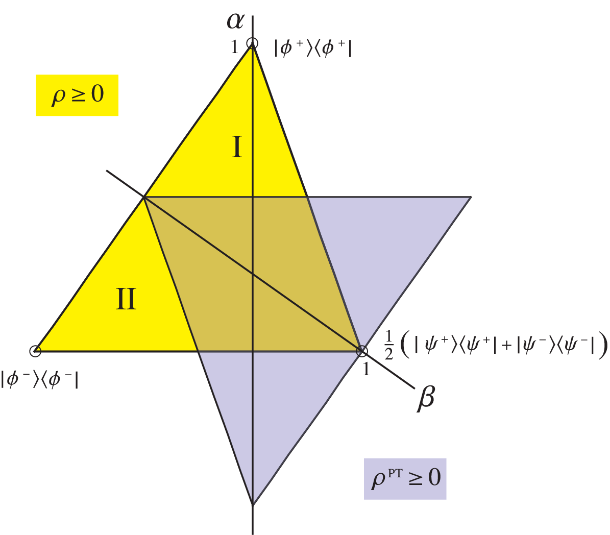
The states (183) are characterized by the two parameters $\alpha$ and $\beta$ and we will refer to the states as the two–parameter states. Of course, the positivity requirement $\rho_{\alpha,\beta}\geq 0$ constrains the possible values of $\alpha$ and $\beta$ , namely

\alpha\;\leq\;-\beta+1,\quad\;\alpha\;\geq\;\frac{1}{3}\beta-\frac{1}{3},\quad\;\alpha\;\leq\;\beta+1\,,

(184)

which geometrically corresponds to a triangle, see Fig. 2.

According to Peres Peres 1996 and the Horodeckis Horodecki et al. 1996a the separability of the states is determined by the positive partial transposition criterion (PPT), at least in dimensions $2\otimes 2$ and $2\otimes 3\,$ . States (183) which are positive under partial transposition have the following constraints

\alpha\;\geq\;\beta-1,\quad\;\alpha\;\leq\;\frac{1}{3}\beta+\frac{1}{3},\quad\;\alpha\geq-\beta-1\,,

(185)

and correspond to the rotated triangle; then the overlap, a rhombus, represents the separable states, see Fig. 2.

In the picture drawn in Fig. 2 the orthogonal lines are indeed orthogonal in HS space. Therefore the coordinate axes for the parameter $\alpha$ and $\beta$ are necessarily non–orthogonal. In particular, the $\alpha$ axis has to be orthogonal to the boundary line $\alpha=-\beta-1$ , and the $\beta$ axis has to be orthogonal to $\alpha=\beta+1$ .

The two–parameter states $\rho_{\alpha,\beta}$ define a plane in the HS space. It is quite illustrative to see how this plane is located in the 3–dimensional spin space of the density matrices, where the 4 Bell states form a tetrahedron due to the positivity condition Bertlmann et al. 2002; Vollbrecht and Werner 2001; Horodecki et al. 1996b. Applying PPT the tetrahedron is rotated producing an intersection —a double pyramid— which represents the separable states. This is shown in Fig. 3.

To calculate the HS measure (167) for the two–parameter qubit state (183) we express the state in terms of the Pauli matrix basis, which is indeed just the GGB and equivalent to the WOB for dimension $d=2$ (see Sec. V.1)

\rho_{\alpha,\beta}\;=\;\frac{1}{4}\left(\mathbbm{1}\,+\,\alpha\left(\sigma_{1}\otimes\sigma_{1}\,-\,\sigma_{2}\otimes\sigma_{2}\right)\,+\,\left(\alpha-\beta\right)\sigma_{3}\otimes\sigma_{3}\right)\,,

(186)

where we have used the well–known Pauli matrix decomposition of the Bell states (see, e.g., Ref. Bertlmann et al. 2002).

In order to determine the HS measure for the entangled two–parameter states $\rho_{\alpha,\beta}^{\rm{ent}}$ we have to find the nearest separable states, which is usually the most difficult task to perform in this context. In Ref. Bertlmann et al. 2005 a lemma is presented to check if a particular separable state is indeed the nearest separable state to a given entangled one:

Lemma 1.

A state $\tilde{\rho}$ is equal to the nearest separable state $\rho_{0}$ if and only if the operator

\tilde{C}\;=\;\frac{\tilde{\rho}-\rho_{\rm ent}\,-\,\left\langle\tilde{\rho},\tilde{\rho}-\rho_{\rm ent}\right\rangle\mathbbm{1}}{\left\|\tilde{\rho}-\rho_{\rm ent}\right\|}

(187)

is an entanglement witness.

Lemma 1 is used here in the following way. First, we calculate the separable state that has the nearest Euclidean distance in the geometric picture (Fig. 2) and call this state $\tilde{\rho}$ . But since the regarded picture does not represent the full state space (e.g., states containing terms like $a_{i}\,\sigma^{i}\otimes\mathbbm{1}$ or $b_{i}\,\mathbbm{1}\otimes\sigma^{i}$ are not contained on the picture), we have to use Lemma 1 to check if the estimated state $\tilde{\rho}$ is indeed the nearest separable state $\rho_{0}$ .

VII.2.1 Region I

Let us consider first the entangled states located in the triangle region that includes the Bell state $|\phi^{+}\rangle\,$ , i.e. Region I in Fig. 2. For $\beta=0$ the states represent the isotropic state (150), thus all results have to agree in this case with Eqs. (174)–(177) for $d=2$ . An entangled state in Region I is characterized by points, i.e. by the parameter pair ( $\alpha$ , $\beta$ ), constrained by

\alpha\;\leq\;\beta+1,\quad\;\alpha\;\leq\;-\beta+1,\quad\;\alpha\;>\;\frac{1}{3}\beta+\frac{1}{3}\,.

(188)

The point in the separable region of Fig. 2 that is nearest (in the Euclidean sense) to the point ( $\alpha$ , $\beta$ ) is given by ( $\frac{1}{3}+\frac{1}{3}\beta$ , $\beta$ ), which corresponds to the state

\tilde{\rho}_{\beta}\;=\;\frac{1}{4}\left(\mathbbm{1}\,+\,\frac{1+\beta}{3}\,\left(\sigma_{1}\otimes\sigma_{1}\,-\,\sigma_{2}\otimes\sigma_{2}\right)\,+\,\frac{1-2\beta}{3}\,\sigma_{3}\otimes\sigma_{3}\right)\,.

(189)

For the difference of nearest–separable and entangled state we obtain

\tilde{\rho}_{\beta}\,-\,\rho^{\rm{ent}}_{\alpha,\beta}\;=\;\frac{1}{4}\left(\frac{1+\beta}{3}\,-\,\alpha\right)\Sigma\,,

(190)

where $\Sigma$ is defined by

\Sigma\;:=\;\sigma_{1}\otimes\sigma_{1}\,-\,\sigma_{2}\otimes\sigma_{2}\,+\,\sigma_{3}\otimes\sigma_{3}\,.

(191)

Using the norm $\|\Sigma\|=2\sqrt{3}$ we gain the HS distance

\|\tilde{\rho}_{\beta}-\rho_{\alpha,\beta}^{\rm{ent}}\|\;=\;\frac{\sqrt{3}}{2}\left(\alpha-\frac{1}{3}-\frac{1}{3}\beta\right)\,.

(192)

To check whether the state $\tilde{\rho}_{\beta}$ coincides with the nearest separable state $\rho_{0;\beta}$ in the sense of the HS measure of entanglement (167) (which has to take into account the whole set of separable states), we have to test —according to Lemma 1— whether the operator

\tilde{C}\;=\;\frac{\tilde{\rho}_{\beta}-\rho^{\rm{ent}}_{\alpha,\beta}\,-\,\langle\tilde{\rho}_{\beta},\tilde{\rho}_{\beta}-\rho^{\rm{ent}}_{\alpha,\beta}\rangle\,\mathbbm{1}}{\|\tilde{\rho}_{\beta}-\rho_{\alpha,\beta}^{\rm{ent}}\|}

(193)

is an entanglement witness. Remember that any entanglement witness $A$ that detects the entanglement of a state $\rho^{\rm{ent}}$ has to satisfy the inequalities (VII.1).

We calculate

\langle\tilde{\rho}_{\beta},\tilde{\rho}_{\beta}-\rho^{\rm{ent}}_{\alpha,\beta}\rangle\;=\;\textnormal{Tr}\,\tilde{\rho}_{\beta}(\tilde{\rho}_{\beta}-\rho^{\rm{ent}}_{\alpha,\beta})\;=\;-\frac{1}{4}\left(\alpha-\frac{1}{3}-\frac{1}{3}\beta\right)

(194)

and use Eqs. (190) and (192) to determine the operator $\tilde{C}$ for the considered case,

\tilde{C}\;=\;\frac{1}{2\sqrt{3}}\,\left(\mathbbm{1}\,-\,\Sigma\right)\,.

(195)

Then we find

\langle\rho^{\rm{ent}}_{\alpha,\beta},\tilde{C}\rangle\;=\;-\frac{\sqrt{3}}{2}\left(\alpha-\frac{1}{3}-\frac{1}{3}\beta\right)\;<\;0\,,

(196)

since the entangled states in the considered Region I satisfy the constraint $\alpha>\frac{1}{3}{\beta}+\frac{1}{3}\,$ . Thus the first condition of inequalities (VII.1) is fulfilled.

Actually, condition (196) is just a consistency check for the correct calculation of operator $\tilde{C}$ since by construction of $\tilde{C}$ we always have $\langle\rho^{\rm{ent}},\tilde{C}\rangle\;=\;-\|\tilde{\rho}-\rho^{\rm{ent}}\|\;<\;0\,$ . Thus more important is the test of the second condition of inequalities (VII.1) and in order to do it we need the following lemma:

Lemma 2.

For any Hermitian operator $C$ that is of the form

C\;=\;a\,\left(\mathbbm{1}\,+\,c_{1}\left(\sigma_{x}\otimes\sigma_{x}\,-\,\sigma_{y}\otimes\sigma_{y}\right)\,+\,c_{2}\,\sigma_{z}\otimes\sigma_{z}\right)\qquad a\in\mathbbm{R^{+}},\quad-1\leq c_{i}\leq 1

(197)

the expectation value for all separable states is positive,

\langle\rho,C\rangle\,\geq\,0\qquad\forall\rho\in S\,.

(198)

Proof. Any separable state $\rho$ is a convex combination of product states and thus a separable two–qubit state can be written as the Bloch vector (see Refs. Bertlmann et al. 2002; Bertlmann et al. 2005)

	$\displaystyle\rho\;=\;\sum_{k}p_{k}\,\frac{1}{4}\left(\mathbbm{1}\otimes\mathbbm{1}\,+\,\sum_{i}n_{i}^{k}\,\sigma^{i}\otimes\mathbbm{1}\,+\,\sum_{j}m_{j}^{k}\,\mathbbm{1}\otimes\sigma^{j}\,+\,\sum_{i,j}n_{i}^{k}m_{j}^{k}\,\sigma^{i}\otimes\sigma^{j}\right)\,,$
	$\displaystyle\textrm{with}\quad n_{i}^{k},m_{i}^{k}\in\mathbbm{R}\,,\;\left\|\vec{n}^{k}\right\|\leq 1\,,\left\|\vec{m}^{k}\right\|\leq 1\,,\ \ p_{k}\geq 0,\,\sum_{k}p_{k}=1\,.$		(199)

Performing the trace we obtain

\langle\rho,C\rangle\;=\;\textnormal{Tr}\,\rho\,C\;=\;\sum_{k}p_{k}\,a\left(1\,+\,c_{1}\left(n_{x}^{k}m_{x}^{k}\,-\,n_{y}^{k}m_{y}^{k}\right)\,+\,c_{2}\,n_{z}^{k}m_{z}^{k}\right)\,.

(200)

We have

\left|c_{1}\left(n_{x}^{k}m_{x}^{k}\,-\,n_{y}^{k}m_{y}^{k}\right)\,+\,c_{2}\,n_{z}^{k}m_{z}^{k}\right|\;\leq\;|n_{x}^{k}||m_{x}^{k}|+|n_{y}^{k}||m_{y}^{k}|+|n_{z}^{k}||m_{z}^{k}|\;\leq\;1\,,

(201)

and therefore

\langle\rho,C\rangle\;\geq\;0\qquad\forall\rho\in S\,.\quad\Box

(202)

Since the operator $\tilde{C}$ (195) is of the form (197) we can use Lemma 2 to verify

\langle\rho,\tilde{C}\rangle\;\geq\;0\qquad\forall\rho\in S\,.

(203)

Therefore $\tilde{C}$ (195) is indeed an entanglement witness and $\tilde{\rho}_{\beta}$ is the nearest separable state $\tilde{\rho}_{\beta}=\rho_{0;\,\beta}$ for the entangled states $\rho_{\alpha,\beta}^{\rm{ent}}$ in Region I.

Finally, we find for the HS measure of the states in Region I

D(\rho_{\alpha,\beta}^{\rm{ent}})\;=\;\|\rho_{0;\,\beta}\,-\,\rho_{\alpha,\beta}^{\rm{ent}}\|\;=\;\frac{\sqrt{3}}{2}\left(\alpha-\frac{1}{3}-\frac{1}{3}\beta\right)\,.

(204)

VII.2.2 Region II

It remains to determine the HS measure for the entangled states $\rho_{\alpha,\beta}^{\rm{ent}}$ located in the triangle region that includes the Bell state $|\phi^{-}\rangle\,$ , i.e. Region II in Fig. 2. Here the entangled states are characterized by points $(\alpha,\beta)\,$ , where the parameters are constrained by

\alpha\;\leq\;\beta+1,\quad\;\alpha\;\geq\;\frac{1}{3}\beta-\frac{1}{3},\quad\;\alpha\;<\;-\beta-1\,.

(205)

The states in the separable region of Fig. 2 that are nearest to the entangled states $(\alpha,\beta)$ in Region II are called $\tilde{\rho}_{\alpha,\beta}$ and characterized by the points

\left(\begin{array}[]{c}\tilde{\alpha}\\ \tilde{\beta}\end{array}\right)\;=\;\left(\begin{array}[]{c}1/3\,\left(-1+2\alpha-\beta\right)\\ 1/3\,\left(-2-2\alpha+\beta\right)\end{array}\right)\,.

(206)

The necessary quantities for calculating the operator $\tilde{C}$ are the following

\tilde{\rho}_{\alpha,\beta}-\rho_{\alpha,\beta}^{\rm{ent}}\;=\;-\frac{1}{12}\left(\alpha+1+\beta\right)\left(\sigma_{x}\otimes\sigma_{x}-\sigma_{y}\otimes\sigma_{y}-\sigma_{z}\otimes\sigma_{z}\right)\,,

(207)

\|\tilde{\rho}_{\alpha,\beta}-\rho_{\alpha,\beta}^{\rm{ent}}\|\;=\;\frac{1}{2\sqrt{3}}\left(-\alpha-1-\beta\right)\,,

(208)

\langle\tilde{\rho}_{\alpha,\beta},\tilde{\rho}_{\alpha,\beta}^{\rm{ent}}-\rho_{\alpha,\beta}\rangle\;=\;\frac{1}{12}\left(\alpha+1+\beta\right)\,,

(209)

so that $\tilde{C}$ is expressed by

\tilde{C}\;=\;\frac{1}{2\sqrt{3}}\left(\mathbbm{1}\,+\,\sigma_{1}\otimes\sigma_{1}\,-\,\sigma_{2}\otimes\sigma_{2}\,-\,\sigma_{3}\otimes\sigma_{3}\right)\,.

(210)

To test $\tilde{C}$ for being an entanglement witness we need to check the first condition of inequalities (VII.1); we get

\langle\rho_{\alpha,\beta}^{\rm{ent}},\tilde{C}\rangle\;=\;\frac{1}{2\sqrt{3}}\left(\alpha+1+\beta\right)\;<\;0

(211)

as expected. Since operator $\tilde{C}$ (210) is of the form (197) we apply Lemma 2 and obtain for the separable states

\langle\rho,\tilde{C}\rangle\;\geq\;0\qquad\forall\rho\in S\,.

(212)

Therefore also in Region II operator $\tilde{C}$ (210) is indeed an entanglement witness and $\tilde{\rho}_{\alpha,\beta}$ is the nearest separable state $\tilde{\rho}_{\alpha,\beta}=\rho_{0;\,\alpha\beta}$ for the entangled states $\rho_{\alpha,\beta}^{\rm{ent}}$ .

For the HS measure of the states in Region II we find

D(\rho_{\alpha,\beta}^{\rm{ent}})\;=\;\|\rho_{0;\,\alpha,\beta}\,-\,\rho_{\alpha,\beta}^{\rm{ent}}\|\;=\;\frac{1}{2\sqrt{3}}\left(-\alpha-1-\beta\right)\,.

(213)

VII.3 Two–parameter entangled states — qutrits

The procedure of determining the geometry of separable and entangled states discussed in Sec. VII.2 can be generalized to higher dimensions, e.g. for two–qutrit states. Let us first notice how to generalize the concept of a maximally entangled Bell basis to higher dimensions. A basis of maximally entangled two–qudit states can be attained by starting with a maximally entangled qudit state $|\phi_{0}\rangle$ and constructing the other $d^{2}-1$ states in the following way:

|\phi_{i}\rangle\;=\;\tilde{U}_{i}\otimes\mathbbm{1}\,|\phi_{0}\rangle\qquad i=1,2,\ldots,d^{2}-1\,,

(214)

where $\{\tilde{U}_{i}\}$ represents an orthogonal matrix basis (1) of unitary matrices and $\tilde{U}_{0}$ usually denotes the unity matrix $\mathbbm{1}$ (see Refs. Vollbrecht and Werner 2000; Werner 2001).

A reasonable choice to start with is the maximally entangled state $|\phi_{+}^{d}\rangle$ (151) and using the WOB (see Sec. V) which is an orthogonal basis of unitary matrices. Such a construction has been proposed in Ref. Narnhofer 2006. Then we set up the following $d^{2}$ projectors onto the maximally entangled states – the Bell states:

P_{nk}\;:=\;(U_{nk}\otimes\mathbbm{1})\,|\phi_{+}^{d}\rangle\langle\phi_{+}^{d}|\,(U_{nk}^{\dagger}\otimes\mathbbm{1})\qquad n,k=0,1,\ldots,d-1\,.

(215)

We can express the Bell projectors as Bloch vectors by using the Bloch vector form (164) of $P_{00}:=|\phi_{+}^{d}\rangle\langle\phi_{+}^{d}|$ and the relations (indices have to be taken $mod\,d$ ) Narnhofer 2006

	$\displaystyle U_{nm}^{\dagger}$	$\displaystyle\;=\;$	$\displaystyle e^{\frac{2\pi i}{d}nm}\,U_{-n\,-k}\,,$		(216)
	$\displaystyle U_{nm}U_{lk}$	$\displaystyle\;=\;$	$\displaystyle e^{\frac{2\pi i}{d}ml}\,U_{n+l\,m+k}\,.$		(217)

It provides for the Bell projector the Bloch form

P_{nk}\;=\;\frac{1}{d^{2}}\sum_{m,l=0}^{d-1}e^{\frac{2\pi i}{d}(kl-nm)}\,U_{lm}\otimes U_{-lm}\,.

(218)

In case of qutrits ( $d=3$ ) the 9 Bell projectors (218) form an 8–dimensional simplex which is the higher dimensional analogue of a 3–dimensional simplex, the tetrahedron for qubits, see Fig. 3. This 8–dimensional simplex has a very interesting geometry concerning separability and entanglement (see Refs. Baumgartner et al. 2006; Baumgartner et al.). Due to its high symmetry inside —named therefore the magic simplex by the authors of Ref. Baumgartner et al. 2006— it is enough to consider certain mixtures of Bell states which form equivalent classes concerning their geometry.

We are interested in the following two–parameter states of two–qutrits as a generalization of the qubit case, Eq. (183),

\rho_{\alpha,\beta}\;=\;\frac{1-\alpha-\beta}{9}\,\mathbbm{1}\,+\,\alpha\,P_{00}\,+\,\beta\frac{1}{2}\left(P_{10}+P_{20}\right)\,.

(219)

According to Ref. Baumgartner et al. 2006 the Bell states represent points in a discrete phase space. The indices $n,k$ of the Bell states can be interpreted as “quantized” position coordinate and momentum, respectively. The Bell states $P_{00},P_{10}$ and $P_{20}$ lie on a line in this phase space picture of the maximally entangled states, they exhibit the same geometry as other lines since each line can be transformed into another one.

Inserting the Bloch vector form of $P_{00},P_{10}$ and $P_{20}$ (218) we find the Bloch vector expansion of the two–parameter states (219)

\rho_{\alpha,\beta}\;=\;\frac{1}{9}\left(\mathbbm{1}\,+\,\left(\alpha-\frac{\beta}{2}\right)U_{1}\,+\,\left(\alpha+\beta\right)U_{2}\right)\,,

(220)

where we defined

	$\displaystyle U_{1}$	$\displaystyle\;:=\;$	$\displaystyle U_{01}\otimes U_{01}+U_{02}\otimes U_{02}+U_{11}\otimes U_{-11}+U_{12}\otimes U_{-12}+U_{21}\otimes U_{-21}+U_{22}\otimes U_{-22}\,,$
	$\displaystyle U_{2}$	$\displaystyle\;:=\;$	$\displaystyle U_{10}\otimes U_{-10}\,+\,U_{20}\otimes U_{-20}\,.$		(221)

The constraints for the positivity requirement ( $\rho_{\alpha,\beta}\geq 0$ ) are

\alpha\;\leq\;\frac{7}{2}\beta+1,\quad\;\alpha\;\leq\;-\beta+1,\quad\;\alpha\;\geq\;\frac{\beta}{8}-\frac{1}{8}\,,

(222)

and for the PPT

\alpha\;\leq\;-\beta-\frac{1}{2},\quad\;\alpha\;\geq\;\frac{5}{4}\beta-\frac{1}{2},\quad\;\alpha\;\leq\;\frac{\beta}{8}+\frac{1}{4}\,.

(223)

The Euclidean picture representing the HS space geometry of states (219) is shown in Fig. 4, where the parameter coordinate axes are non–orthogonal since in HS space they have to be orthogonal to the boundary lines of the positivity region, $\alpha=\frac{\beta}{8}-\frac{1}{8}$ and $\alpha=\frac{7}{2}\beta+1$ .

It is shown in Ref. Baumgartner et al. 2006 that the PPT states $\rho_{\alpha,\beta}$ are all separable states, so there are no bound entangled PPT states of the form (219). To find the HS measure for the entangled two–parameter 2–qutrit states we apply the same procedure as in Sec. VII.2: We determine the states that are the nearest separable ones in the Euclidean sense of Fig. 4 and use Lemma 1 to check whether these are indeed the nearest separable ones with respect to the whole state space (for other approaches see, e.g., Refs. Verstraete et al. 2002; Cao and Wang 2007).

VII.3.1 Region I

First we consider Region I in Fig. 4, i.e., the triangle region of entangled states around the $\alpha$ -axis, constrained by the parameter values

\alpha\;\leq\;\frac{7}{2}\beta+1,\quad\;\alpha\leq-\beta+1,\quad\;\alpha>\frac{\beta}{8}+\frac{1}{4}\,.

(224)

In the Euclidean picture the point that is nearest to point $(\alpha,\beta)$ in this region is given by $(\frac{1}{4}+\frac{1}{8}\beta,\beta)$ , which corresponds to the separable two–qutrit state

\tilde{\rho}_{\beta}\;=\;\frac{1}{9}\left(\mathbbm{1}\,+\,\left(\frac{1}{4}-\frac{3}{8}\beta\right)U_{1}\,+\,\left(\frac{1}{4}+\frac{9}{8}\beta\right)U_{2}\right)\,,

(225)

with $U_{1}$ and $U_{2}$ defined in Eq. (VII.3).

For the difference of nearest–separable and entangled state we find

\tilde{\rho}_{\beta}-\rho^{\rm{ent}}_{\alpha,\beta}\;=\;\frac{1}{9}\left(\frac{1}{4}+\frac{1}{8}\beta-\alpha\right)U\,,

(226)

where $U=U_{1}+U_{2}$ (and is defined in Eq. (165)), and using for the norm $\|U\|=d\sqrt{8}=6\sqrt{2}$ we gain the HS distance

\|\tilde{\rho}_{\beta}-\rho_{\alpha,\beta}^{\rm{ent}}\|\;=\;\frac{2\sqrt{2}}{3}\left(\alpha-\frac{1}{4}-\frac{1}{8}\beta\right)\,.

(227)

It remains to calculate

\langle\tilde{\rho}_{\beta},\tilde{\rho}_{\beta}-\rho_{\alpha,\beta}\rangle\;=\;\textnormal{Tr}\,\tilde{\rho}_{\beta}(\tilde{\rho}_{\beta}-\rho_{\alpha,\beta})\;=\;-\frac{2}{9}\left(\alpha-\frac{1}{4}+\frac{1}{8}\beta\right)

(228)

to set up the operator

\tilde{C}\;=\;\frac{\tilde{\rho}_{\beta}-\rho^{\rm{ent}}_{\alpha,\beta}\,-\,\langle\tilde{\rho}_{\beta},\tilde{\rho}_{\beta}-\rho^{\rm{ent}}_{\alpha,\beta}\rangle\,\mathbbm{1}}{\|\tilde{\rho}_{\beta}-\rho_{\alpha,\beta}^{\rm{ent}}\|}\;=\;\frac{1}{6\sqrt{2}}\,\left(2\,\mathbbm{1}\,-\,U\right)\,.

(229)

We test now whether it represents an entanglement witness, i.e., whether $\tilde{C}$ (229) satisfies the inequalities (VII.1). As expected we find

\langle\rho^{\rm{ent}}_{\alpha,\beta},\tilde{C}\rangle\;=\;-\frac{2\sqrt{2}}{3}\left(\alpha-\frac{1}{4}-\frac{1}{8}\beta\right)\;<\;0\,.

(230)

To check the second condition of inequalities (VII.1) we set up the following lemma, similar to Lemma 2:

Lemma 3.

For any Hermitian operator $C$ that is of the form

C\;=\;a\,(2\,\mathbbm{1}\,+\,c_{1}\,U_{1}\,+\,c_{2}\,U_{2})\qquad a\in\mathbbm{R^{+}},\quad-1\leq c_{i}\leq 1

(231)

the expectation value for all separable states is positive,

\langle\rho,C\rangle\;\geq\;0\qquad\forall\rho\in S\,.

(232)

Proof. Any separable two–qutrit state can be written as the Bloch vector Bertlmann et al. 2002; Bertlmann et al. 2005

$\displaystyle\rho$	$\displaystyle\;=\;$	$\displaystyle\sum_{k}p_{k}\ \frac{1}{9}\Big(\mathbbm{1}\otimes\mathbbm{1}\,+\,\sum_{n,m=0}^{d-1}\sqrt{2}\,n_{nm}^{k}\,U_{nm}\otimes\mathbbm{1}\,+\,\sum_{l,k=0}^{d-1}\sqrt{2}\,m_{lk}^{k}\,\mathbbm{1}\otimes U_{lk}$	(233)
		$\displaystyle\,+\,\sum_{n,m,l,k=0}^{d-1}2\,n_{nm}^{k}m_{lk}^{k}\,U_{nm}\otimes U_{lk}\Big)\,,$
		$\displaystyle\textrm{with}\quad n_{nm}^{k},m_{lk}^{k}\in\mathbbm{C}\,,\;\left\|\vec{n}^{k}\right\|\leq 1\,,\left\|\vec{m}^{k}\right\|\leq 1\,,\;\ p_{k}\geq 0,\,\sum_{k}p_{k}=1\,,$

where we define $\left|\vec{n}^{k}\right|^{2}:=\sum_{nm}n_{nm}^{*}n_{nm}\,$ .

Performing the trace we obtain

\langle\rho,C\rangle\;=\;\textnormal{Tr}\,\rho^{\dagger}\,C\;=\;\sum_{k}p_{k}\left(2a\left(1\,+\,c_{1}\sum_{i=1}^{6}n_{i}^{k}m_{i}^{k}\,+\,\sum_{j=7}^{8}c_{2}n_{j}^{k}m_{j}^{k}\right)\right)\,,

(234)

with

	$\displaystyle\left(n_{1},n_{2},n_{3},n_{4},n_{5},n_{6},n_{7},n_{8}\right)$	$\displaystyle\;=\;$	$\displaystyle\left(n_{01}^{},n_{02}^{},n_{11}^{},n_{12}^{},n_{21}^{},n_{22}^{},n_{10}^{},n_{20}^{}\right)\mbox{ and}$
	$\displaystyle\left(m_{1},m_{2},m_{3},m_{4},m_{5},m_{6},m_{7},m_{8}\right)$	$\displaystyle\;=\;$	$\displaystyle\left(m_{01}^{},m_{02}^{},m_{-11}^{},m_{-12}^{},m_{-21}^{},m_{-22}^{},m_{-10}^{},m_{-20}^{}\right).$

We have

\left|c_{1}\sum_{i=1}^{6}n_{i}^{k}m_{i}^{k}\,+\,c_{2}\sum_{j=7}^{8}n_{j}^{k}m_{j}^{k}\right|\;\leq\;\sum_{i}|n_{i}^{k}||m_{i}^{k}|\;\leq\;1

(236)

and therefore

\langle\rho,C\rangle\;\geq\;0\qquad\forall\rho\in S\,.\quad\Box

(237)

Since the operator $\tilde{C}$ (229) is of the form (231) we can use Lemma 3 to verify

\langle\rho,\tilde{C}\rangle\;\geq\;0\qquad\forall\rho\in S\,.

(238)

Thus $\tilde{C}$ (229) is indeed an entanglement witness and $\tilde{\rho}_{\beta}$ is the nearest separable state $\tilde{\rho}_{\beta}=\rho_{0;\,\beta}$ for the entangled states $\rho_{\alpha,\beta}^{\rm{ent}}$ in Region I.

For the HS measure of the entangled two–parameter two–qutrit states (219) we find

D(\rho_{\alpha,\beta}^{\rm{ent}})\;=\;\|\rho_{0;\,\beta}-\rho_{\alpha,\beta}^{\rm{ent}}\|\;=\;\frac{2\sqrt{2}}{3}\left(\alpha-\frac{1}{4}-\frac{1}{8}\beta\right)\,.

(239)

VII.3.2 Region II

In Region II of Fig. 4 the entangled two–parameter two–qutrit states are constrained by

\alpha\;<\;\frac{5}{4}\beta-\frac{1}{2},\quad\;\alpha\;\geq\;\frac{1}{8}\beta-\frac{1}{8},\quad\;\alpha\;\leq\;-\beta+1\,.

(240)

The points that have minimal Euclidean distance to the points $(\alpha,\beta)$ located in this region are characterized by

\left(\begin{array}[]{c}\tilde{\alpha}\\ \tilde{\beta}\end{array}\right)=\left(\begin{array}[]{c}1/24\,\left(-2+20\alpha+5\beta\right)\\ 1/6\,\left(2+4\alpha+\beta\right)\end{array}\right)\,,

(241)

and correspond to the states $\tilde{\rho}_{\alpha,\beta}$ . The quantities needed for calculating $\tilde{C}$ are

$\displaystyle\tilde{\rho}_{\alpha,\beta}\,-\,\rho_{\alpha,\beta}^{\rm{ent}}$	$\displaystyle\;=\;$	$\displaystyle-\frac{1}{72}\left(4\alpha+2-5\beta\right)\left(U_{1}-U_{2}\right)\,,$	(242)
$\displaystyle\\|\tilde{\rho}_{\alpha,\beta}-\rho_{\alpha,\beta}^{\rm{ent}}\\|$	$\displaystyle\;=\;$	$\displaystyle\frac{1}{6\sqrt{2}}\left(-4\alpha-2+5\beta\right)\,,$	(243)
$\displaystyle\langle\tilde{\rho}_{\alpha,\beta},\tilde{\rho}_{\alpha,\beta}^{\rm{ent}}-\rho_{\alpha,\beta}\rangle$	$\displaystyle\;=\;$	$\displaystyle\frac{1}{36}\left(4\alpha+2-5\beta\right)\,,$	(244)

so that operator $\tilde{C}$ is expressed by

\tilde{C}\;=\;\frac{1}{6\sqrt{2}}\,\left(2\,\mathbbm{1}\,+\,U_{1}\,-\,U_{2}\right)\,.

(245)

The check of the first condition (VII.1) for an entanglement witness gives, unsurprisingly,

\langle\rho_{\alpha,\beta}^{\rm{ent}},\tilde{C}\rangle\;=\;\frac{1}{6\sqrt{2}}\,\left(4\alpha+2-5\beta\right)\,<\,0\,,

(246)

since $4\alpha<5\beta-2\,$ , Eq. (240). For the second test we use the fact that operator $\tilde{C}$ (245) is of the form (231) and thus, according to Lemma 3, we obtain

\langle\rho,\tilde{C}\rangle\;\geq\;0\qquad\forall\rho\in S\,.

(247)

Therefore $\tilde{C}$ (245) is indeed an entanglement witness and the states $\tilde{\rho}_{\alpha,\beta}$ are the nearest separable ones $\tilde{\rho}_{\alpha,\beta}=\rho_{0;\,\alpha,\beta}$ to the entangled two–parameter states (219) of Region II.

Finally, for the HS measure of these states we obtain

D(\rho_{\alpha,\beta}^{\rm{ent}})\;=\;\|\rho_{0;\,\alpha,\beta}\,-\,\rho_{\alpha,\beta}^{\rm{ent}}\|\;=\;\frac{1}{6\sqrt{2}}\,\left(-4\alpha-2+5\beta\right)\,.\\

(248)

VIII Conclusion

In this paper we present three different matrix bases which are quite useful to decompose density matrices for higher dimensional qudits. These are the generalized Gell-Mann matrix basis GGB, the polarization operator basis POB, and the Weyl operator basis WOB. Each decomposition we identify with a vector, the so-called Bloch vector.

Considering just one–particle states we observe the following features:

The GGB is easy to construct, the matrices correspond to the standard SU(N) generators ( $N=d$ ), but in general (in $d$ dimensions) it is rather unpractical to work with the diagonal GGM (5) due to its more complicated definition. On the other hand, the Bloch vector itself has real components, which is advantageous, they can be expressed as expectation values of measurable quantities. For example, in $3$ dimensions the Gell-Mann matrices are Hermitian and the Bloch vector components can be expressed by expectation values of spin 1 operators. The POB is also easy to set up, all you need to know are the Clebsch–Gordan coefficients which you find tabulated in the literature. However, the Bloch vector contains complex components. The Weyl operators for the WOB are also simple to construct, they are non–Hermitian but unitary operators. The Bloch vector itself turns out very simple, however, with complex components. Let us note that in $2$ dimensions all bases are equivalent since they correspond to Pauli matrices or linear combinations thereof.

In case of two–qudits we have studied the isotropic states explicitly and find the following characteristics:

In the GGB the Bloch vector (158) with expression (159) is more complicated to construct, in particular the diagonal part $B$ (156) (see Appendix A.2). In the POB the Bloch vector (163) with expression (162) can be easily set up by the knowledge of the Clebsch–Gordon coefficient sum rule (160) and in the WOB the Bloch vector (166) with definition (165) is actually most easily to construct.

The Hilbert–Schmidt measure of entanglement has been calculated explicitly for the isotropic two–qudit states and we want to emphasize its connection to the maximal violation of a generalized Bell inequality (Theorem 1), an inequality for the entanglement witness.

We demonstrate the geometry of separability and entanglement in case of qubits by choosing so-called two–parameter states, Eq. (183), i.e., planes in the tetrahedron formed by the Bell states (see Fig. 3). These states reflect already the underlying geometry of the Hilbert Space and they are chosen with regard to the description of qutrit states, a generalization into higher dimensions. To a given entangled state we determine the nearest separable state, calculate the corresponding entanglement witness and the Hilbert–Schmidt measure in the relevant Regions I and II (see Fig. 2).

In case of qutrits it is quite illustrative to demonstrate the geometry of separability and entanglement in terms of two–parameter states (219). These states set up a plane in the 8–dimensional simplex formed by the $9$ Bell states and are easy to construct within the WOB. Due to the high symmetry of the magic simplex we may restrict ourselves to a certain mixture of Bell states, Eq. (219), which exhibits the same geometry as other lines. Within the WOB it is quite easy to find the Bloch vector form (220) of the two–parameter states. It is straightforward to find for a given entangled state in the relevant Regions I and II (see Fig. 4) the nearest separable state and the corresponding entanglement witness. The easy calculation of the Hilbert–Schmidt measure of entanglement is a great advantage in this case and its result of high interest since it is quite difficult to calculate other entanglement measures for higher dimensional states, like the entanglement of formation.

It turns out that the Weyl operator basis is optimal for all our calculations, the reason is that entanglement —the maximally entangled Bell states— is in fact easily constructed by unitary operators à la Weyl.

Acknowledgements.

We would like to thank Heide Narnhofer, Beatrix Hiesmayr, Alexander Ableitinger and Marcus Huber for helpful discussion and comments. This research has been supported by the “F140-N Forschungsstipendium” of the University of Vienna.

Appendix A

A.1 Proof of Orthogonality of GGB

We want to proof condition (1) for the GGB which consists of the $d^{2}-1$ GGM (3), (4), (5) and the $d\times d$ unity $\mathbbm{1}$ . Since all GGM are Hermitian (thus $\textnormal{Tr}A_{i}^{{\dagger}}A_{j}=\textnormal{Tr}A_{i}A_{j}=\textnormal{Tr}A_{j}A_{i}$ ) it suffices to proof the following conditions:

$\displaystyle\textnormal{Tr}\,\Lambda^{jk}_{s}\Lambda^{mn}_{s}$	$\displaystyle\;=\;$	$\displaystyle 2\,\delta^{jm}\delta^{kn}$	(249)
$\displaystyle\textnormal{Tr}\,\Lambda^{jk}_{a}\Lambda^{mn}_{a}$	$\displaystyle\;=\;$	$\displaystyle 2\,\delta^{jm}\delta^{kn}$	(250)
$\displaystyle\textnormal{Tr}\,\Lambda^{l}\Lambda^{m}$	$\displaystyle\;=\;$	$\displaystyle 2\,\delta^{lm}$	(251)
$\displaystyle\textnormal{Tr}\,\Lambda^{jk}_{a}\Lambda^{mn}_{s}$	$\displaystyle\;=\;$	$\displaystyle 0$	(252)
$\displaystyle\textnormal{Tr}\,\Lambda^{jk}_{s}\Lambda^{m}$	$\displaystyle\;=\;$	$\displaystyle 0$	(253)
$\displaystyle\textnormal{Tr}\,\Lambda^{jk}_{a}\Lambda^{m}$	$\displaystyle\;=\;$	$\displaystyle 0\,.$	(254)

Proof of condition (249). Inserting definition (3) we have

$\displaystyle\textnormal{Tr}\,\Lambda^{jk}_{s}\Lambda^{mn}_{s}$	$\displaystyle\;=\;$	$\displaystyle\sum_{l=1}^{d}\langle l\|\left(\|j\rangle\langle k\|\,+\,\|k\rangle\langle j\|\right)\left(\|m\rangle\langle n\|\,+\,\|n\rangle\langle m\|\right)\|l\rangle$	(255)
	$\displaystyle\;=\;$	$\displaystyle\sum_{l}\left(\langle l\|j\rangle\langle k\|m\rangle\langle n\|l\rangle\,+\,\langle l\|j\rangle\langle k\|n\rangle\langle m\|l\rangle\,+\,\langle l\|k\rangle\langle j\|m\rangle\langle n\|l\rangle\,+\,\langle l\|k\rangle\langle j\|n\rangle\langle m\|l\rangle\right)$
	$\displaystyle\;=\;$	$\displaystyle\delta^{jn}\delta^{km}\,+\,\delta^{jm}\delta^{kn}\,+\,\delta^{kn}\delta^{jm}\,+\,\delta^{km}\delta^{jn}$
	$\displaystyle\;=\;$	$\displaystyle 2\,\delta^{jm}\delta^{kn}\,,$

where we used in the last step that $\delta^{jn}\delta^{km}=0$ since we have $j<k$ and $m<n$ .

Proof of condition (250). This case is equivalent to the one before apart from changed signs that do not matter

	$\displaystyle\textnormal{Tr}\,\Lambda^{jk}_{a}\Lambda^{mn}_{a}$	$\displaystyle\;=\;$	$\displaystyle-\,\delta^{jn}\delta^{km}\,+\,\delta^{jm}\delta^{kn}\,+\,\delta^{kn}\delta^{jm}\,-\,\delta^{km}\delta^{jn}$		(256)
		$\displaystyle\;=\;$	$\displaystyle 2\,\delta^{jm}\delta^{kn}\,.$		(256)

Proof of condition (251). Using definition (5) and denoting

C_{l}=\sqrt{\frac{2}{l(l+1)}}\,,

(257)

where $l\leq m$ without loss of generality, we get

$\displaystyle\textnormal{Tr}\,\Lambda^{l}\Lambda^{m}$	$\displaystyle\;=\;$	$\displaystyle C_{l}C_{m}\sum_{p=1}^{d}\Big(\sum_{k=1}^{l}\sum_{n=1}^{m}\langle p\|k\rangle\langle k\|n\rangle\langle n\|p\rangle\,+\,lm\langle p\|l+1\rangle\langle l+1\|m+1\rangle\langle m+1\|p\rangle$	(258)
		$\displaystyle-\,m\sum_{k=1}^{l}\langle p\|k\rangle\langle k\|m+1\rangle\langle m+1\|p\rangle\,-\,l\sum_{n=1}^{m}\langle p\|l+1\rangle\langle l+1\|n\rangle\langle n\|p\rangle\Big)$
	$\displaystyle\;=\;$	$\displaystyle C_{l}C_{m}\left(l\,+\,lm\,\delta^{lm}\,-\,m\sum_{k=1}^{l}\delta^{k(m+1)}\,-\,l\sum_{n=1}^{m}\delta^{n(l+1)}\right)\,.$

Using the fact that $\delta^{k(m+1)}=0$ for $m\geq k$ and

l\sum_{n=1}^{m}\delta^{n(l+1)}\;=\;\begin{cases}0&\text{if}\ l=m\\ l&\text{if}\ l<m\end{cases}

(259)

we obtain

\textnormal{Tr}\,\Lambda^{l}\Lambda^{m}\;=\;(C_{l})^{2}\,l(l+1)\,\delta^{lm}\;=\;2\,\delta^{lm}\,.

(260)

Proof of condition (252). Analogously to the proofs (255) and (256) we find

\textnormal{Tr}\,\Lambda^{jk}_{a}\Lambda^{mn}_{s}\;=\;i\left(-\,\delta^{jn}\delta^{km}\,+\,\delta^{jm}\delta^{kn}\,-\,\delta^{jm}\delta^{kn}\,+\,\delta^{jn}\delta^{km}\right)\;=\;0\,.

(261)

Proof of condition (253). Inserting definitions (3) and (5) gives

$\displaystyle\text{Tr}\,\Lambda^{jk}_{s}\Lambda^{m}$	$\displaystyle\;=\;$	$\displaystyle C_{m}\sum_{p=1}^{d}\Big(-m\langle p\|k\rangle\langle j\|m+1\rangle\langle m+1\|p\rangle\,-\,m\langle p\|j\rangle\langle k\|m+1\rangle\langle m+1\|p\rangle$	(262)
		$\displaystyle+\sum_{n=1}^{m}\langle p\|j\rangle\langle k\|n\rangle\langle n\|p\rangle\,+\,\sum_{n=1}^{m}\langle p\|k\rangle\langle j\|n\rangle\langle n\|p\rangle\Big)$
	$\displaystyle\;=\;$	$\displaystyle-\,2m\,\delta^{j(m+1)}\delta^{k(m+1)}\,+\,2\sum_{l=1}^{m}\delta^{kl}\delta^{jl}$
	$\displaystyle\;=\;$	$\displaystyle 0\,,$

since per definition we have $j<k\,$ .

Proof of condition (254). This proof is equivalent to the previous one since constant factors in front of the terms do not matter.

A.2 Calculation of term B in GGB

To obtain the Bloch vector notation of term $B$ (154) we insert the standard matrix expansion (90) for the case $j=k$ . We split the tensor products in the following way

B\;=\;\frac{1}{d}\left(B_{1}\,+\,B_{2}\,+\,B_{3}\,+\,B_{4}\,+\,\frac{1}{d}\,\mathbbm{1}\otimes\mathbbm{1}\right)\,,

(263)

where the terms $B_{1},\ldots,B_{4}$ are introduced by (note that $\Lambda^{0}=0$ )

$\displaystyle B_{1}$	$\displaystyle\;=\;$	$\displaystyle\sum_{j=1}^{d}\left(\frac{j-1}{2j}\Lambda^{j-1}\otimes\Lambda^{j-1}\,+\,\sum_{n(=l)=0}^{d-j-1}\frac{1}{2(j+n)(j+n+1)}\Lambda^{j+n}\otimes\Lambda^{j+n}\right)$	(264)
$\displaystyle B_{2}$	$\displaystyle\;=\;$	$\displaystyle\sum_{j=1}^{d}\Bigg(-\sum_{l=0}^{d-j-1}\sqrt{\frac{j-1}{4j(j+l)(j+l+1)}}\Lambda^{j-1}\otimes\Lambda^{j+l}$	(265)
		$\displaystyle\qquad\ \,-\sum_{n=0}^{d-j-1}\sqrt{\frac{j-1}{4j(j+n)(j+n+1)}}\Lambda^{j+n}\otimes\Lambda^{j-1}$
		$\displaystyle\qquad\ \,+\sum_{n\neq l,\,n,l=0}^{d-j-1}\frac{1}{2\sqrt{(j+n)(j+n+1)(j+l)(j+l+1)}}\Lambda^{j+n}\otimes\Lambda^{j+l}\Bigg)$
$\displaystyle B_{3}$	$\displaystyle\;=\;$	$\displaystyle\frac{1}{d}\sum_{j=1}^{d}\left(-\sqrt{\frac{j-1}{2j}}\Lambda^{j-1}\otimes\mathbbm{1}\,+\,\sum_{n=0}^{d-j-1}\frac{1}{\sqrt{2(j+n)(j+n+1)}}\Lambda^{j+n}\otimes\mathbbm{1}\right)$	(266)
$\displaystyle B_{4}$	$\displaystyle\;=\;$	$\displaystyle\frac{1}{d}\sum_{j=1}^{d}\left(-\sqrt{\frac{j-1}{2j}}\mathbbm{1}\otimes\Lambda^{j-1}\,+\,\sum_{l=0}^{d-j-1}\frac{1}{\sqrt{2(j+l)(j+l+1)}}\mathbbm{1}\otimes\Lambda^{j+l}\right)\,.$	(267)

Only the first term $B_{1}$ (264) gives a contribution

B_{1}\;=\;\sum_{m=1}^{d-1}\left(\frac{m}{2(m+1)}\,+\,\frac{m}{2m(m+1)}\right)\Lambda^{m}\otimes\Lambda^{m}\;=\;\frac{1}{2}\sum_{m=1}^{d-1}\Lambda^{m}\otimes\Lambda^{m}\,,

(268)

whereas the remaining terms vanish:

$\displaystyle B_{2}$	$\displaystyle\;=\;$	$\displaystyle\sum_{m<p,\,m,p=1}^{d-1}\left(-\sqrt{\frac{m}{4(m+1)p(p+1)}}\,+\,\frac{m}{\sqrt{4m(m+1)p(p+1)}}\right)\Lambda^{m}\otimes\Lambda^{p}$	(269)
		$\displaystyle+\sum_{m>p,\,m,p=1}^{d-1}\left(-\sqrt{\frac{p}{4(p+1)m(m+1)}}\,+\,\frac{p}{\sqrt{4p(p+1)m(m+1)}}\right)\Lambda^{m}\otimes\Lambda^{p}$
	$\displaystyle\;=\;$	$\displaystyle\left(\sum_{m<p}\frac{-m+m}{2\sqrt{m(m+1)p(p+1)}}\,+\,\sum_{m>p}\frac{-p+p}{2\sqrt{m(m+1)p(p+1)}}\right)\Lambda^{m}\otimes\Lambda^{p}$
	$\displaystyle\;=\;$	$\displaystyle 0\,,$

and in quite the same manner

	$\displaystyle B_{3}$	$\displaystyle\;=\;$	$\displaystyle\frac{1}{d}\sum_{m=1}^{d-1}\frac{-m+m}{\sqrt{2m(m+1)}}\ \Lambda^{m}\otimes\mathbbm{1}=0\,,$
	$\displaystyle B_{4}$	$\displaystyle\;=\;$	$\displaystyle\frac{1}{d}\sum_{p=1}^{d-1}\frac{-p+p}{\sqrt{2p(p+1)}}\ \mathbbm{1}\otimes\Lambda^{p}=0\,.$		(270)

Thus we find the following Bloch vector of $B$ (154)

B\;=\;\frac{1}{2d}\sum_{m=1}^{d-1}\Lambda^{m}\otimes\Lambda^{m}\,+\,\frac{1}{d^{2}}\,\mathbbm{1}\otimes\mathbbm{1}\,.

(271)

A.3 Proof of Orthonormality of WOB

For proofs relevant in the WOB we often need the equivalence

\sum_{n=0}^{d-1}e^{\frac{2\pi i}{d}\,nx}\;=\;\begin{cases}d&\text{if }x=0\\ 0&\text{if }x\neq 0\end{cases},\quad x\in\mathbbm{Z}\,.

(272)

So we use Eq. (272) to proof the orthonormality of the Weyl operators (141)

$\displaystyle\text{Tr}\,U_{nm}^{{\dagger}}U_{lj}$	$\displaystyle\;=\;$	$\displaystyle\sum_{p=0}^{d-1}\sum_{k,\tilde{k}=0}^{d-1}e^{\frac{2\pi i}{d}\,(\tilde{k}l-kn)}\,\langle p\|(k+m)\,\textrm{mod}\,d\rangle\langle k\|\tilde{k}\rangle\langle(\tilde{k}+j)\,\textrm{mod}\,d\|p\rangle$	(273)
	$\displaystyle\;=\;$	$\displaystyle\sum_{p=0}^{d-1}\sum_{k,\tilde{k}=0}^{d-1}e^{\frac{2\pi i}{d}\,(\tilde{k}l-kn)}\,\langle p\|(k+m)\,\textrm{mod}\,d\rangle\langle(\tilde{k}+j)\,\textrm{mod}\,d\|p\rangle\,\delta_{k\tilde{k}}$
	$\displaystyle\;=\;$	$\displaystyle\sum_{k=0}^{d-1}e^{\frac{2\pi i}{d}\,k(l-n)}\,\delta_{mj}$
	$\displaystyle\;=\;$	$\displaystyle d\,\delta_{nl}\,\delta_{mj}\,.$

A.4 Expansion into WOB

Formula (164) for the Bell state in terms of WOB we derive in the following way. We express the standard matrices by the WOB (147), rewrite the indices and separate the nonvanishing terms

$\displaystyle\left\|\phi_{+}^{d}\right\rangle\left\langle\phi_{+}^{d}\right\|$	$\displaystyle\;=\;$	$\displaystyle\frac{1}{d}\sum_{j,k=1}^{d}\|j\rangle\langle k\|\otimes\|j\rangle\langle k\|$	(274)
	$\displaystyle\;=\;$	$\displaystyle\frac{1}{d^{3}}\sum_{j,k=0}^{d-1}\sum_{l,l^{\prime}=0}^{d-1}e^{-\frac{2\pi i}{d}\,j(l+l^{\prime})}U_{l(k-j)mod\,d}\otimes U_{l^{\prime}(k-j)mod\,d}$
	$\displaystyle\;=\;$	$\displaystyle\frac{1}{d^{3}}\sum_{m,k=0}^{d-1}\sum_{l,l^{\prime}=0}^{d-1}e^{-\frac{2\pi i}{d}\,(k-m)(l+l^{\prime})}U_{lm}\otimes U_{l^{\prime}m}$
	$\displaystyle\;=\;$	$\displaystyle\frac{1}{d^{2}}\left(\sum_{m}U_{0m}\otimes U_{0m}\,+\,\sum_{m}\,\sum_{l,l^{\prime};\,l+l^{\prime}=d}U_{lm}\otimes U_{l^{\prime}m}\right)$
		$\displaystyle+\;\frac{1}{d^{3}}\sum_{m}\,\sum_{l,l^{\prime};\,l,l^{\prime}\neq 0,0;\,l+l^{\prime}\neq d}\left(\sum_{k}e^{-\frac{2\pi i}{d}\,(k-m)(l+l^{\prime})}\right)U_{lm}\otimes U_{l^{\prime}m}\,.$

The last term in Eq. (274) vanishes due to relation (272). Identifying $U_{00}=\mathbbm{1}$ and using the notation with negative values of the index $l$ , which have to be considered as $mod\ d\,$ , we gain the formula

\left|\phi_{+}^{d}\right\rangle\left\langle\phi_{+}^{d}\right|\;=\;\frac{1}{d^{2}}\,\mathbbm{1}\otimes\mathbbm{1}\,+\,\frac{1}{d^{2}}\,\sum_{l,m=0}^{d-1}U_{lm}\otimes U_{-lm}\,,\qquad(l,m)\neq(0,0)\,.

(275)

References

Bloch (1946) F. Bloch, Phys. Rev. 70, 460 (1946).
Nielsen and Chuang (2000) M. Nielsen and I. Chuang, Quantum Computation and Quantum Information (Cambridge University Press, Cambridge, England, 2000).
Kimura (2003) G. Kimura, Phys. Lett. A 314, 339 (2003).
(4) S. Kryszewski and M. Zachciał, quant-ph/0602065.
Jakobczyk and Siennicki (2001) L. Jakobczyk and M. Siennicki, Phys. Lett. A 286, 383 (2001).
Kimura and Kossakowski (2005) G. Kimura and A. Kossakowski, Open Sys. Information Dyn. 12, 207 (2005).
Mendaš (2006) I. P. Mendaš, J. Phys. A: Math. Gen. 39, 11313 (2006).
Witte and Trucks (1999) C. Witte and M. Trucks, Phys. Lett. A 257, 14 (1999).
Ozawa (2000) M. Ozawa, Phys. Lett. A 268, 158 (2000).
Bertlmann et al. (2002) R. A. Bertlmann, H. Narnhofer, and W. Thirring, Phys. Rev. A 66, 032319 (2002).
Bertlmann et al. (2005) R. A. Bertlmann, K. Durstberger, B. C. Hiesmayr, and P. Krammer, Phys. Rev. A 72, 052331 (2005).
(12) C. Rakotonirina, math.GM/0511451.
Caves and Milburn (2000) C. M. Caves and G. J. Milburn, Optics Communications 179, 439 (2000).
Varshalovich et al. (1988) D. A. Varshalovich, A. N. Moskalev, and V. K. Khersonskii, Quantum theory of angular momentum (World Scientific Publishing Co. Pte. Ltd., 1988).
Bennett et al. (1993) C. H. Bennett, G. Brassard, C. Crépeau, R. Jozsa, A. Peres, and W. K. Wootters, Phys. Rev. Lett. 70, 1895 (1993).
Narnhofer (2006) H. Narnhofer, J. Phys. A: Math. Gen. 39, 7051 (2006).
Baumgartner et al. (2006) B. Baumgartner, B. C. Hiesmayr, and H. Narnhofer, Phys. Rev. A 74, 032327 (2006).
Werner (2001) R. F. Werner, J. Phys. A: Math. Gen. 34, 7081 (2001).
Vollbrecht and Werner (2000) K. G. H. Vollbrecht and R. F. Werner, J. Math. Phys. 41, 6772 (2000).
Henley and Thirring (1962) E. M. Henley and W. Thirring, Elementary Quantum Field Theory (McGraw Hill, New York, 1962).
Horodecki and Horodecki (1999) M. Horodecki and P. Horodecki, Phys. Rev. A 59, 4206 (1999).
Rains (1999) E. M. Rains, Phys. Rev. A 60, 179 (1999).
Horodecki et al. (2001) M. Horodecki, P. Horodecki, and R. Horodecki, in Quantum Information, edited by G. A. et al. (Springer Verlag Berlin, 2001), vol. 173 of Springer Tracts in Modern Physics, p. 151.
Horodecki et al. (1996a) M. Horodecki, P. Horodecki, and R. Horodecki, Phys. Lett. A 223, 1 (1996a).
Terhal (2000) B. M. Terhal, Phys. Lett. A 271, 319 (2000).
Terhal (2002) B. M. Terhal, Theoretical Computer Science 287, 313 (2002).
Peres (1996) A. Peres, Phys. Rev. Lett. 77, 1413 (1996).
Vollbrecht and Werner (2001) K. G. H. Vollbrecht and R. F. Werner, Physical Review A 64, 062307 (2001).
Horodecki et al. (1996b) M. Horodecki, P. Horodecki, and R. Horodecki, Phys. Rev. A 54, 1838 (1996b).
(30) B. Baumgartner, B. C. Hiesmayr, and H. Narnhofer, arXiv:0705.1403.
Verstraete et al. (2002) F. Verstraete, K. Audenaert, and B. D. Moor, J. Mod. Opt. 49, 1277 (2002).
Cao and Wang (2007) Y. Cao and A. M. Wang, J. Phys. A: Math. Theor. 40, 3507 (2007).