Dynamical conductance in the two-channel Kondo regime of a double dot system
Abstract
We study finite-frequency transport properties of the double-dot system recently constructed to observe the two-channel Kondo effect [R. M. Potok et al., Nature 446, 167 (2007)]. We derive an analytical expression for the frequency-dependent linear conductance of this device in the Kondo regime. We show how the features characteristic of the 2-channel Kondo quantum critical point emerge in this quantity, which we compute using the results of conformal field theory as well as numerical renormalization group methods. We determine the universal cross-over functions describing non-Fermi liquid vs. Fermi liquid cross-overs and also investigate the effects of a finite magnetic field.
pacs
72.15.Qm, 73.21.La, 73.23.-b, 73.23.Hk, 73.43.Nq, 73.63.KvI Introduction
In the past few years semiconducting quantum dots have been in the focus of intense research. This research has mostly been motivated by their possible application in future microelectronics: these devices behave as tunable artificial atoms attached to electrodes,QD_review they can be used as single electron transistors,SET furthermore they also serve as a playground to model and study (artificial) molecular transport in a very controlled way. They display a number of correlation-induced effects like the Coulomb blockade or the Kondo effectCB; Kondo and they can also give rise to exotic strongly correlated states.SU4 Very importantly, quantum dots can also be used to build quantum bits with the electron spin providing the necessary degree of freedom for quantum-computation.Loss
Nevertheless, maybe the most fascinating application of quantum dots is their possible use to realize quantum phase transitions between different correlated states. Several such transitions have been proposed: under special circumstances the transition between the triplet and the singlet state of a dot can be a true quantum phase transition,SchollerHofstetter; GoldhaberST although in most cases this transition becomes just a cross-over.WanderViel Dissipation can also lead to a quantum phase transition where the charge degrees of freedom of the dot become localized.LeHur; Simon Unfortunately, these phase transitions have a Kosterlitz-Thouless structure and are – in a sense – ’trivial’ quantum phase transitions. Using multi-dot systems, however, it is also possible to realize generic quantum phase transitions, where the transition point represents a true critical state characterized by anomalous dimensions and a singular behavior. These critical states are generic non-Fermi liquid states in the sense that they cannot be described in terms of conduction electron quasiparticles even at the Fermi energy.Nozieres The prototypes of these generic quantum impurity states are the two-channel Kondo modelCox and the two-impurity Kondo model.2imp Some years ago Matveev proposed that the two-channel Kondo model could be realized by charge fluctuations at the charge-degeneracy point of a quantum dot.Matveev However, Matveev’s mapping assumes a vanishing level spacing and with present-day technology it has been impossible to reach this state so far. However, a few years ago Oreg and Goldhaber-Gordon proposed to realize the two-channel Kondo state through a double dot system,Oreg and after several years of work this two-channel Kondo state has indeed been observed in a pioneering double dot experiment at Stanford.Potok For the realization of the other prototypical non-Fermi liquid state, the two-impurity Kondo state, a somewhat similar multi-dot setup has been proposed recently.chung
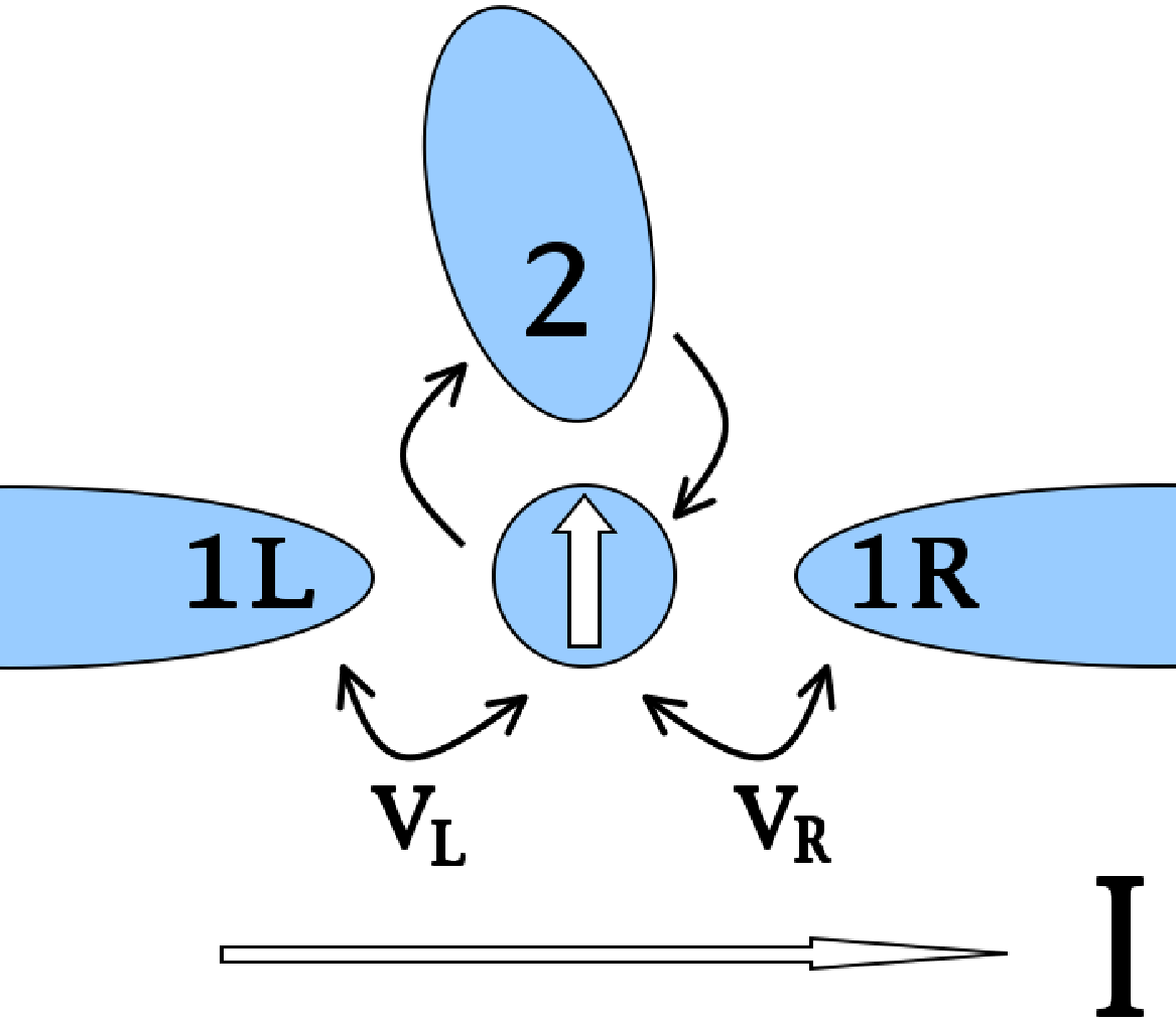
Fig. 1 shows the double dot device suggested by Oreg and Goldhaber-Gordon, which has since been used to experimentally reach the two-channel Kondo fixed point Potok. This set-up consist of a small dot coupled to a large dot (2) and two leads ( and ). The small dot is tuned to the regime where charge fluctuations are suppressed and it has only one extra electron on it. The level spacing, , of the small dot and its charging energy are assumed to be much larger than the temperature, , so that below the scale charge fluctuations on the small dot are suppressed and the only role of this dot is to provide a spin. The size of the large dot, on the other hand, is chosen in such a way that its charging energy and level spacing satisfy . This implies that this dot is also in the Coulomb blockade regime while the electronic states on it form a continuum of electron-hole excitations. Therefore, electrons on the large dot form a bath that can exchange spin with the small dot while electrons cannot jump out of itOreg as it is also indicated in Fig. 1. In the limit of small tunneling amplitudes, apart from some irrelevant and potential scattering terms, this double dot system is described by the following simple two-channel Kondo Hamiltonian,
| (1) |
The operator describes electrons on the large dot. In the continuum limit, , it is defined as
| (2) |
with the annihilation operator of a conduction electron of energy and spin on the large dot, satisfying the anticommutation relation: . The operator in Eq. (1) is a suitably chosen linear combination of electrons on the left and right lead-electrodes,
| (3) |
with and the hopping amplitudes between the dot and the left and right electrodes, respectively. The left and right fields are defined similarly to Eq. (2),
| (4) |
with the annihilation operator of a conduction electron of energy and spin on the left/right lead.
We remark that, strictly speaking, the Kondo Hamiltonian above is only accurate in the limit of small tunneling, while in the experiments the tunneling rates were quite large in order to boost up the Kondo temperature.Potok Therefore, to study the region far above , an Anderson model-type approach would be needed that also accounts for charge fluctuations of the small dot.Anders Nevertheless, our Kondo model-based approach captures accurately the universal cross-over functions in the region of interest, i.e. around and far below the Kondo temperature, provided that both dots are close to the middle of the Coulomb blockade regime. To account for deviations from the middle of the Coulomb blockade valley, one could break the particle-hole symmetry of Eq. (1) and add potential scattering terms to it.


The quantum critical state arises as a result of the competition of channels 1 and 2 to form a singlet with the dot spin . Depending on the values of the dimensionless couplings, , two situations can occur:Oreg; Cox (a) For the spin of the small dot forms a Kondo singlet with electrons on the large dot that screen the spin at an energy scale . In this case, to promote a conduction electron between the left and right leads one needs to break up the Kondo singlet and pay an energy , and therefore transport through the small dot is suppressed at low temperatures.Oreg; Potok (b) For , on the other hand, the spin of the small dot is screened by electrons in the leads. This correlated singlet state serves as a ’bridge’ and helps the lead electrons to propagate between the left and the right sides with a small reflection probability and is thus characterized by a conductance of the order of the quantum conductance, . In both cases a Fermi liquid state is formed below the scale , which can be characterized by simple phase shifts at the Fermi energy.Nozieres
Interestingly, for the scale vanishes as , and a non-Fermi liquid state emerges below the Kondo scale, , with the cut-off defined as .Cox This so-called two-channel Kondo state is characterized by a conductance that is about half of the quantum conductance at very low temperatures, and has a singularity for .Oreg This state is – in a sense – a quantum critical state: although it is just a single point in the parameter space, it separates two stable Fermi-liquid phases, and it influences the behavior of the double dot system over the whole regime, for . However, as we shall see later, the scaling properties usually associated with the two-channel Kondo fixed point itself are restricted to a somewhat smaller energy range, . The characteristic features of the temperature-dependence of the DC conductance and the schematic phase diagram are sketched in Fig. 2.
The purpose of the present paper is to investigate dynamical transport properties of the above set-up and determine how the two-channel Kondo behavior and the presence of a quantum critical point at manifests itself in the AC conductance through the dot. For this purpose, we shall derive an expression for the AC conductance in the linear response regime that relates the conductance to the so-called composite Fermions’ propagator at any temperature and frequency. Making use of this simple formula, we shall evaluate the AC conductance for frequencies using numerical renormalization group methods. We shall also determine the universal cross-over functions that describe the non-Fermi liquid vs. Fermi liquid cross-over for . As we show, the AC conductance exhibits features that are qualitatively similar to the finite temperature DC conductance, sketched in Fig. 2. In addition, we shall also investigate, what conclusions we can draw regarding AC properties based upon the predictions of conformal field theory, and use this approach to obtain the universal scaling of the conductance in the regime .
The paper is organized as follows. Section II provides the details of the derivation of the AC conductance formula for the two-channel Kondo model. In Section III we present some analytical considerations based on conformal field theory concerning the universal scaling properties of the linear conductance and of the eigenvalue of the so-called on-shell -matrix. Section IV comprises our numerical renormalization group results for the composite Fermions’ spectral function and the linear conductance in case of channel anisotropy and in the presence of a magnetic field. At last our conclusions are summarized.
II Kubo formula and composite Fermions
Let us start our analysis with the derivation of a simple expression for the AC conductance in terms of the so-called composite Fermion operators.Theo For this purpose, we first couple an external voltage to the dot and introduce a time-dependent chemical potential difference between the left and right electrodes:
| (5) |
with and the number of electrons in the left and right leads, respectively,
The current operator can be defined as the time derivative of , . This commutator is easily shown to give
| (6) |
where denotes the decoupled electron field of the leads,
| (7) |
and we have introduced the so-called composite Fermion operator,
| (8) |
The operator has spin 1/2 and charge 1, and it corresponds to the ’universal part’ of the electron localized on the small dot.
Close to equilibrium, the current through the dot is given by the Kubo formula
| (9) |
with the conductance. Differentiating with respect to time and then taking the Fourier transform we obtain the relation
| (10) |
where denotes the retarded current-current correlation function and is a real constant
| (11) |
Thus the real and imaginary parts of the conductance are given by
| (12) | |||||
| (13) |
In general, it is not so simple to compute the correlation function . In our case, however, the field is completely decoupled from the spin and describes non-interacting Fermions. This observation allows us to write as
| (14) |
where , , , and denote the usual retarded, advanced, bigger and lesser Keldysh Green’s functions. The Fourier transform of this expression simplifies considerably if one uses the fact that the field is non-interacting and therefore the corresponding Green’s functions become in the large band-width limit
| (15) |
with the Fermi function. Taking the real and imaginary parts of the Fourier transform of Eq. (14) we finally obtain:
| (16) | |||||
| (17) |
where we introduced the dimensionless eigenvalue of the so-called on-shell -matrix,dephasing_2 which describes the scattering of electrons of energy ,
| (18) |
and denotes the maximum conductance through the dot,
| (19) |
Thus the real part of the conductance is related to the imaginary part of , which is essentially the spectral function of the composite Fermion, . The latter can be determined numerically using the numerical renormalization group method. Then the real part, , can be obtained by performing a Hilbert transformation numerically, and the imaginary part of the conductance can then be calculated from by simple numerical integration. Note that Eqs. (16) and (17) provide the linear conductance through the dot for any asymmetry parameter at any temperature and any frequency. They are thus natural extensions of the formula given in Ref. PustilnikGlazman?, and are the analogues of the formulas obtained recently for the Anderson model.sindel05
III Analytical considerations
Eq. (16) allows us to make numerous statements based on rather general properties of the two-channel Kondo fixed point.Cox From an exact theorem of Affleck and Ludwig,AffleckLudwig e.g. we know that at the two-channel Kondo fixed point (i.e. for and ) the -matrix of the conduction electrons identically vanishes. From the relation, between the dimensionless eigenvalue of the -matrix and the -matrix we thus obtain
| (20) |
From this, it immediately follows that at the two-channel Kondo fixed point the conductance takes half of its maximum value,
| (21) |
The results of conformal field theoryAffleckLudwig also enable us to compute the finite frequency conductance for and . In this limit the -matrix is given by the expressionAffleckLudwig
| (22) |
where is the hypergeometric function, and stands for the amplitude of the leading irrelevant operator:
| (23) |
The value of the dimensionless constant depends on the precise definition of . Throughout this paper, we shall define as the energy at which for the composite Fermion’s spectral function drops to half of its value, . Then, comparing the numerical results of Section IV to the asymptotic behavior of the conductance we obtain the value . Clearly, since the omega-dependence enters only in the combination , it immediately follows that is a universal function of (see inset of Fig. 3).
In Fig. 3 we show the results obtained by numerically integrating Eq.(22) for a few temperatures. It is remarkable that curves corresponding to different temperatures cross each-other. This feature is a direct consequence of the unusual shape of the universal curve shown in the inset of Fig. 3.

Note that to construct the universal scaling curve one needs to rescale the axes with respect to the temperature only, and the precise value of the Kondo temperature appears only through the prefactor . The fact that the only relevant energy scale is the temperature is characteristic of quantum critical points. The imaginary part of the -matrix exhibits a cusp for , and crosses over to a quadratic regime for . Similar behavior is observed in the real part of , shown in Fig. 4. This quantity also shows a characteristic behavior at frequencies , that crosses over to a linear regime for .

Using Eqs.(22), Eqs.(16) and (17), both the real and the imaginary parts of the conductance can be computed by numerical integration. The results are plotted in Figs. 5 and 6 for various temperatures. Even though, at first sight, the results for the conductivity look qualitatively similar to those for the -matrix, there is an important difference: integration with the Fermi functions apparently eliminated the aforementioned crossing of the curves. Similar scaling curves have been computed using conformal field theory results for the differential conductance of two-channel Kondo scatterers in point contacts.vonDelftLudwigAmbegaokar


In the limit, , the conformal field theory also predicts that the AC conductance scales as
| (24) |
with a universal constant of order of unity. The fact that the coefficients in the two equations above are both equal to , follows from the observation that is analytical in the upper half-plane.
For a new Fermi liquid scale, (mentioned earlier), emerges, but one can still make many statements based upon the fact that the leading relevant and irrelevant operators have scaling dimensions and , respectively.Cox As a consequence, in the vicinity of the two-channel Kondo fixed point () the conductance becomes a function of the form:
| (25) |
with the Fermi liquid scale approximately given by
| (26) |
where we introduced the renormalized anisotropy parameter as
| (27) |
Throughout this paper we shall define as the energy scale at which in the channel of larger coupling. Note that the parameter can be considerably larger than the naive estimate, due to the renormalization of the couplings and in the high energy regime, . In the limit of and the conductance becomes a universal function of ,
| (28) |
The signs refer to the cases and , respectively, and the scaling functions have the properties
| (29) |
In other words, for the conductance through the dot is Fermi liquid like, and shows a behavior, while for the real part of the conductance scales to its two-channel Kondo value with a small but increasing correction, . The latter behavior breaks down once the amplitude of the leading irrelevant operator, , reaches that of the anisotropy operator, , i.e. at frequencies in the range . The constants , , and above are numbers of order unity that depend somewhat on electron-hole symmetry breaking, but close to electron-hole symmetry , and . Note that the precise value of the constants and depends also on the definition of the scale .
The imaginary part of has somewhat different properties and behaves as
| (30) |
In other words, the imaginary part of must show a bump of size at frequencies . These expectations shall indeed be met by our numerical results.
Similar to channel asymmetry, an external magnetic field also suppresses the non-Fermi liquid behavior,Cox and introduces a new Fermi liquid scale,
| (31) |
However, the magnetic field does not result in such a dramatic change in the conductance as the channel-symmetry breaking: while at the conductance exhibits a jump as a function of the channel-anisotropy, it changes continuously as a function of the magnetic field and shows only a cusp,LaciGlazman; Anders
| (32) |
as it obviously follows from the singular behavior of the conduction electron phase shifts at the Fermi energy.AffleckLudwigPangCox; LaciGlazman As we shall see later, the AC conductance displays much more interesting features in a finite magnetic field.
IV Numerical results

In this section, we shall use the numerical renormalization group (NRG) methodNRG_ref to compute the eigenvalue of the -matrix and from that the AC conductance. Although Eqs. (16) and (17) hold at any temperature, finite temperature calculations are extremely delicate close to a non-Fermi liquid state. Therefore, we shall present numerical results only for temperature here. Nevertheless, according to the basic principles of scaling, a finite frequency plays a role rather similar to that of a finite temperature, and therefore the temperature AC conductance, , behaves rather similarly to the DC conductance at a finite temperature , .
To perform accurate calculations we assumed an electron-hole symmetrical conduction band and strongly exploited the symmetries of the Hamiltonian. The numerical results presented here have been obtained using a new “flexible” NRG code, that handles symmetries dynamically.Anna In particular, in the absence of an external magnetic field, we used a symmetry , with and the charge symmetries in channels 1 and 2, respectively,Jones and the spin symmetry. The advantage of this symmetry is that it is not violated even for , and it breaks down only to in the presence of a magnetic field. For the channel anisotropic cases we have retained a maximum of 750 multiplets during the NRG calculations, whereas 850 multiplets were kept in the presence of a magnetic field. All calculations were carried out with a discretization parameter . To compute the AC conductance, we have determined the composite Fermion’s spectral function which, apart from an overall normalization factor, is equal to . This normalization factor can be easily fixed for using the condition, Eq. (20). This procedure is much more accurate than estimating the normalization factor from the bare couplings, since the latter procedure suffers from the NRG discretization problem as well as from the loss of spectral weight at high energies, leading generally to a few percent error in the amplitude.
IV.1 Channel symmetry breaking
First we investigated numerically how the non-Fermi liquid structure appears in the AC conductance through the double dot and how channel anisotropy destroys this non-Fermi liquid behavior. Some typical results are shown in Fig. 7: for we recover the two-channel Kondo result, , and the deviation from the fixed point value scales as , in agreement with Eq. (24).

For the new cross-over scale appears below which crosses over from the two-channel Kondo value , to for or to for in the electron-hole symmetrical situation studied numerically. In the limit this cross-over is described by universal cross-over functions, similar to Eq. (29). We determined these scaling functions numerically and displayed them in Fig. 8. (The black curves were obtained by taking an extremely small value of , and chopping off the parts near .) The Fermi liquid scale extracted from is shown in Fig. 7.(c), and is in excellent agreement with the analytical expression, Eq. (26).


According to Eq. (16), the real part of the conductance can be computed from through a simple integration. The resulting conductance curves are shown in Fig. 9. The behavior of is strikingly similar to that of : it also exhibits a singularity for and crosses over from a value to or to at the scale following the universal cross-over functions, . We remark here that there seems to be no other reliable way than NRG to determine these universal cross-over functions, which connect two separate strong coupling fixed points, the non-Fermi liquid liquid fixed point and the Fermi liquid fixed point. These universal cross-over functions constitute some of the central results of this work.
Performing a Hilbert transform, we also determined numerically the real part of the -matrix, , and from that the imaginary part of the conductance. These results are shown in Fig. 10. It is quite remarkable that, although the scaling is not perfect because of the insufficient accuracy of the Hilbert transform and the various integrations, clearly, the amplitude of the low temperature peak at does not change as goes to 0. (Note that varies over two orders of magnitudes.) This behavior is indeed expected based upon Eq. (30). The numerical results confirm that for and the coefficients have different signs, , and , and that has a double peak structure: it has one peak at corresponding to the cross-over to the two-channel Kondo fixed point, and also another peak at related to the non-Fermi liquid Fermi liquid cross-over.
It is interesting to observe from Figs. 8, 9, and 10 that the range of two-channel Kondo scaling does not reach from down to the cross-over scale , but rather it stops at a much higher energy scale, , where corrections from the leading relevant operators start to dominate over the leading irrelevant operator of the two-channel Kondo fixed point.

IV.2 Effects of magnetic field
We also performed calculations for in the presence of a local magnetic field, . As mentioned earlier, a small local magnetic field destroys the non-Fermi liquid state and drives the system to a trivial, Fermi liquid fixed point below a scale .AffleckLudwigPangCox
Some typical results are shown in Fig. 11. At large magnetic fields, , the Kondo resonance is clearly split below the Zeeman field, and exhibits a dip for . The width of this dip gradually decreases as one decreases the size of the field , and its depth becomes smaller and smaller. However, it is not clear from the numerics if there is a critical field value, below which the dip actually disappears, as is the case, e.g. for the single-channel Kondo model. In fact, the numerical results seem to show just the opposite, i.e. that remains a non-monotonous function in any finite magnetic field, and only the height and width of the dip at get smaller and smaller for smaller magnetic fields while the dip itself is always present. This would indeed naturally follow from a simple scaling argument: for a magnetic energy scale is generated, , and at this energy the real part of the conductance is expected to be . On the other hand, from Bethe AnsatzBA we know the exact phase shifts, and from that it immediately follows that the DC conductance is given by at temperature, with a constant of the order of unity.LaciGlazman This observation suggests that in any finite magnetic field displays a dip, which has a width , and height . Similar behavior is expected as a function of temperature, too.
It is not clear either, if becomes a universal function of . In fact, it has been shown in a special, very anisotropic limit that no such universal function exists for the non-linear DC conductance.Schiller We can argue that the same probably holds for the linear AC conductance, although we do not have a rigorous proof.
Unfortunately, from a numerical point of view the calculations in a magnetic field turned out to be extremely difficult: first of all, for the positive and negative frequency parts of the spectral function one looses somewhat different amounts of spectral weight. This effect turns out to be extremely large in the 2-channel Kondo case, probably as a consequence of the extreme sensitivity of the non-Fermi liquid fixed point to the magnetic field. Therefore, for a given spin direction, one needs to match these positive and negative-frequency parts at the origin. Although this is a standard procedure followed by most groups, this leads to a large uncertainty in case of the 2-channel Kondo model. In fact, despite the extensive symmetries used, we were not able to obtain data of sufficient accuracy in the most interesting regime, , even using Hofstetter’s density matrix NRG (DMNRG) method.Hofstetter Therefore, we were not able to investigate the issue of universal cross-over functions for and . We therefore consider these numerical results only as indicative but not decisive.


We also need to recall the well-known fact that NRG produces an artificial broadening proportional to of the peaks occuring at finite frequencies. Thus, the correct shape of these split peaks is presumably significantly sharper than that shown by the NRG results.
V Conclusions
In this paper, we have studied the AC transport properties of a double dot device realized recently by Potok et al. to reach the two-channel Kondo fixed point. First we derived an analytical expression for the linear conductance in the regime where charge fluctuations are small and the system can be described by a Kondo Hamiltonian. Our formula relates the AC conductance to the eigenvalue of the dimensionless on-shell -matrix, and is valid at any temperature and for any frequency. Our expression is the analogue of the formula obtained recently by Sindel et al. for the Anderson modelsindel05 and it carries over to most Kondo-type Hamiltonians.


The general properties of the two-channel Kondo fixed point, known from conformal field theory, allowed us to make many quantitative and qualitative predictions for the AC conductance, : for equal couplings to the two channels, shows an singularity at the two-channel Kondo fixed point. Using the results of conformal field theory,AffleckLudwig we were able to compute the real and imaginary parts of the function and determine the corresponding scaling functions for both the real and the imaginary parts of the conductance through the dot in the universal regime, and . The generic properties of the AC conductance in this regime are summarized in Fig. 12.


Conformal field theory also gave us a way to predict the basic properties of and at temperature, in the presence of channel symmetry-breaking (see Fig. 13). For crosses over to a much smaller or a much larger value (depending on the sign of asymmetry) at the Fermi-liquid scale , below which it becomes an analytical function of . This cross-over at is described by universal cross-over functions that we have determined numerically. The asymptotic properties of the real and imaginary parts of the conductance are dictated by conformal field theory (see Eqs. (29) and (30)). It is quite remarkable that shows a double peak structure at frequencies and . Both peaks are of amplitude but the sign of the peak at changes with the sign of .
One of the important conclusions that one could draw from the analysis of was, that the two-channel Kondo regime is, in a sense, restricted to the regime, : Although it is true that the entire regime, is governed by the 2-channel Kondo fixed point, for the leading relevant operator is more important than the leading irrelevant operator, and therefore, the scaling curves characteristic to the two-channel Kondo fixed point itself cannot be seen in this regime. This refines somewhat the phase diagram of the two-channel Kondo model, as already indicated in Fig. 2. The two-channel Kondo scaling regime is thus limited by a boundary .
We have also investigated the effects of a small Zeeman field on the AC conductance. For the AC conductance exhibits a dip whose width is just . Numerically we find that, apparently, this dip survives for any small magnetic field, . This would indeed be in agreement with a simple scaling argument we presented, that also predicts a similar behavior as a function of temperature. In other words, at the two-channel Kondo fixed point the Kondo resonance appears to be split at any magnetic field. Unfortunately, while our numerics seems to support this picture, it is not accurate enough in the regime, to give a decisive answer. We remark that the logarithmic magnetic field dependence of the phase shift would also probably imply that universal scaling (i.e. scaling and the disappearance of the scale for ) should be destroyed by logarithmic corrections in the presence of magnetic field.
We would like to thank F. Anders, A. Schiller and L. Udvardi for helpful discussions. This research has been supported by Hungarian grants OTKA Nos. NF061726, T046267, T046303, D048665, by the DFG center for functional nanostructures (CFN), and by Sonderforschungsbereich 631. G. Z. acknowledges the hospitality of the CAS, Oslo, and L. B. the financial support received from the Bolyai Foundation.
References
- (1) For a review, see e.g. L. I. Glazman, M. Pustilnik, in ”Nanophysics: Coherence and Transport,” eds. H. Bouchiat et al., pp. 427-478 (Elsevier, 2005).
- (2) For reviews, see e.g. G. Schön and A. D. Zaikin, Phys. Rep. 198, 237 (1990); or G.-L. Ingold and Y. V. Nazarov, in: Single Charge Tunneling, ed. by H. Grabert and M. Devoret, NATO ASI Series B, vol. 294, pp. 21-107 (Plenum, 1992).
- (3) R. Wilkins, E. Ben-Jacob, and R. C. Jaklevic, Phys. Rev. Lett. 63, 801 (1989).
- (4) D. Goldhaber-Gordon, H. Shtrikman, D. Mahalu, D. Abusch-Magder, U. Meirav, and M. A. Kastner, Nature (London) 391, 156 (1998); S. M. Cronenwett, T. H. Oosterkamp and L. P. Kouwenhoven, Science 281, 540 (1998); J. Schmid, J. Weis, K. Eberl, and K. von Klitzing, Physica B 256-258, 182 (1998).
- (5) See, e.g., L. Borda, G. Zaránd, W. Hofstetter, B. I. Halperin, J. von Delft, Phys. Rev. Lett. 90, 026602 (2003).
- (6) D. Loss and D. P. DiVincenzo, Phys. Rev. A 57, 120 (1998).
- (7) W. Hofstetter, H. Schoeller, Phys. Rev. Lett. 88, 016803 (2002).
- (8) A. Kogan, G. Granger, M. A. Kastner, D. Goldhaber-Gordon, H. Shtrikman, Phys. Rev. B 67, 113309 (2003).
- (9) S. Sasaki, S. De Franceschi, J. M. Elzerman, W. G. van der Wiel, M. Eto, S. Tarucha, and L. P. Kouwenhoven, Nature 405, 764 (2000); J. Schmid, J. Weis, K. Eberl, and K. von Klitzing, Phys. Rev. Lett. 84, 5824 (2000).
- (10) M. Pustilnik, L. I. Glazman, W. Hofstetter, Phys. Rev. B 68, 161303(R) (2003); W. Hofstetter, G. Zaránd, Phys. Rev. B 69, 235301 (2004).
- (11) K. Le Hur, Phys. Rev. Lett. 92, 196804 (2004);
- (12) L. Borda, G. Zaránd and P. Simon, Phys. Rev. B 72, 155311 (2005); M.-R. Li, K. Le Hur, and W. Hofstetter, Phys. Rev. Lett. 95, 086406 (2005).
- (13) D. L. Cox and A. Zawadowski, Adv. Phys. 47, 599 (1998).
- (14) B. A. Jones, C. M. Varma, and J. W. Wilkins, Phys. Rev. Lett. 61, 125 (1988); B. A. Jones and C. M. Varma, Phys. Rev. B 40, 324 (1989); J. B. Silva, W. L. Lima, W. C. Oliveira, J. L. Mello, L. N. Oliveira, and J. W. Wilkins, Phys. Rev. Lett. 76 275 (1996).
- (15) K. A. Matveev, Zh. Eksp. Teor. Fiz. 98, 1598 (1990) [Sov. Phys. JETP 72, 892 (1991)]; Phys. Rev. B 51, 1743 (1995).
- (16) Y. Oreg and D. Goldhaber-Gordon, Phys. Rev. Lett. 90, 136602 (2003).
- (17) M. Pustilnik, L. I. Glazman, Phys. Rev. B 64, 045328 (2001).
- (18) R. M. Potok, I. G. Rau, H. Shtrikman, Y. Oreg, D. Goldhaber-Gordon, Nature (London) 446, 167 (2007).
- (19) L. Borda, L. Fritz, N. Andrei and G. Zaránd, arXiv:cond-mat/0703293.
- (20) G. Zaránd, C.-H. Chung, P. Simon, M. Vojta, Phys. Rev. Lett. 97, 166802 (2006).
- (21) T. A. Costi, Phys. Rev. Lett. 85, 1504 (2000).
- (22) W. Hofstetter, Phys. Rev. Lett. 85, 1508 (2000).
- (23) M. Sindel, W. Hofstetter, J. von Delft, and M. Kindermann Phys. Rev. Lett. 94, 196602 (2005).
- (24) Ph. Nozières, J. Low Temp. Phys. 17, 31 (1974).
- (25) M. Pustilnik, L. Borda, L. I. Glazman, J. von Delft, Phys. Rev. B. 69, 115316 (2004).
- (26) A. I. Tóth et al., unpublished.
- (27) F. B. Anders, E. Lebanon, and A. Schiller, Phys. Rev. B 70, 201306 (2004); F. B. Anders, Phys. Rev. B 71, 121101 (2005).
- (28) B. A. Jones, C. M. Varma, and J. W. Wilkins, Phys. Rev. Lett. 61, 125 (1988).
- (29) I. Affleck, A. W. W. Ludwig, H.-B. Pang and D. L. Cox, Phys. Rev. B. 45, 7918 (1992).
- (30) I. Affleck, A. W. W. Ludwig, Phys. Rev. B. 48, 7297 (1993).
- (31) J. von Delft, A. W. W. Ludwig und V. Ambegaokar, Ann. Phys. 273, 175-241 (1998).
- (32) A. Schiller and S. Hershfield, Phys. Rev. B 51, 12896 (1995).
- (33) K. G. Wilson, Rev. Mod. Phys. 47, 773 (1975); for a recent review see R. Bulla, T. A. Costi, T. Pruschke, cond-mat/0701105 (2007).
- (34) N. Andrei, C. Destri, Phys. Rev. Lett. 52, 364 (1984).