ITP-Budapest Report No. 634 Form factors in finite volume I:
form factor bootstrap and truncated conformal space

B. Pozsgay and G. Takács Thanks: E-mail: pozsi@bolyai.elte.hu Thanks: E-mail: takacs@elte.hu Affiliation: Institute for Theoretical PhysicsEötvös University, Budapest Affiliation: HAS Research Group for Theoretical PhysicsH-1117 Budapest, Pázmány Péter sétány 1/A

26th June 2007

Abstract

We describe the volume dependence of matrix elements of local fields to all orders in inverse powers of the volume (i.e. only neglecting contributions that decay exponentially with volume). Using the scaling Lee-Yang model and the Ising model in a magnetic field as testing ground, we compare them to matrix elements extracted in finite volume using truncated conformal space approach to exact form factors obtained using the bootstrap method. We obtain solid confirmation for the form factor bootstrap, which is different from all previously available tests in that it is a non-perturbative and direct comparison of exact form factors to multi-particle matrix elements of local operators, computed from the Hamiltonian formulation of the quantum field theory. We also demonstrate that combining form factor bootstrap and truncated conformal space is an effective method for evaluating finite volume form factors in integrable field theories over the whole range in volume.

1 Introduction

The matrix elements of local operators (form factors) are central objects in quantum field theory. In two-dimensional integrable quantum field theory the $S$ matrix can be obtained exactly in the framework of factorized scattering (see [1, 2] for reviews), and using the scattering amplitudes as input it is possible to obtain a set of axioms satisfied by the form factors [3], which provides the basis for the so-called form factor bootstrap (see [4] for a review).

Although the connection with the Lagrangian formulation of quantum field theory is rather indirect in the bootstrap approach, it is thought that the general solution of the form factor axioms determines the complete local operator algebra of the theory [5]. This expectation was confirmed in many cases by explicit comparison of the space of solutions to the spectrum of local operators as described by the ultraviolet limiting conformal field theory [6, 7, 8, 9]; mathematical foundation is provided by the local commutativity theorem stating that operators specified by solutions of the form factor bootstrap are mutually local [4]. Another important piece of information comes from correlation functions: using form factors, a spectral representation for the correlation functions can be built which provides a large distance expansion [10, 11], while the Lagrangian or perturbed conformal field theory formulation allows one to obtain a short-distance expansion, which can then be compared provided there is an overlap between their regimes of validity [11]. Other evidence for the correspondence between the field theory and the solutions of the form factor bootstrap results from evaluating sum rules like Zamolodchikov’s $c$ -theorem [12, 13] or the $\Delta$ -theorem [14], both of which can be used to express conformal data as spectral sums in terms of form factors. Direct comparisons with multi-particle matrix elements are not so readily available, except for perturbative or $1/N$ calculations in some simple cases [3].

Therefore, part of the motivation of this paper is to provide non-perturbative evaluation of form factors from the Hamiltonian formulation, which then allows for a direct comparison with solutions of the form factor axioms. Another goal is to have a better understanding of finite size effects in the case of matrix elements of local operators, and to contribute to the investigation of finite volume [15] (and also finite temperature [16]) form factors and correlation functions.

Based on what we learned from our previous investigation of decay rates in finite volume [17], in this paper we determine form factors using a formulation of quantum field theory in finite volume. In two space-time dimensions this is most efficiently done using the truncated conformal space approach (TCSA) developed by Yurov and Zamolodchikov [18], but one could have also made use of, for example, lattice field theory: the only important point is to have a method which can be used to determine energy levels and matrix elements of local operators as functions of the volume. We give a relation between finite and infinite volume multi-particle form factors, which is a natural extension of the results by Lellouch and Lüscher for two-particle decay matrix elements [19]. It is used to determine form factors in two important examples of integrable quantum field theory: the scaling Lee-Yang model and the Ising model in a magnetic field. We show that these results agree very well with the predictions of the form factor bootstrap. We only treat matrix elements of local fields between multi-particle states for which there are no disconnected pieces (which appear whenever there are particles with coincident rapidities in the left and right multi-particle states); the treatment of disconnected pieces, together with a number of theoretical arguments and ramifications, are postponed to a subsequent publication [20].

The organization of the paper is as follows. In section 2, after a brief review of necessary facts concerning the form factor bootstrap we give the general description of form factors (without disconnected pieces) to all orders in $1/L$ based on an analysis of two-point correlation functions. Section 3 describes the two models we chose for demonstration, and also specifies the method of evaluating form factors from truncated conformal space. Numerical results on elementary form factors (vacuum–many-particle matrix elements) are given in section 4, while the general case is treated in section 5. We give our conclusions in section 6.

2 Form factors in finite volume

2.1 Form factor bootstrap

Here we give a very brief summary of the axioms of the form factor bootstrap, in order to set up notations and to provide background for later arguments; the interested reader is referred to Smirnov’s review [4] for more details. Let us suppose for simplicity that the spectrum of the model consists of particles $A_{i}$ , $i=1,\dots,N$ with masses $m_{i}$ , which are assumed to be strictly non-degenerate, i.e. $m_{i}\neq m_{j}$ for any $i\neq j$ (and therefore also self-conjugate). Because of integrability, multi-particle scattering amplitudes factorize into the product of pairwise two-particle scatterings, which are purely elastic (in other words: diagonal). This means that any two-particle scattering amplitude is a pure phase, which we denote by $S_{ij}\left(\theta\right)$ where $\theta$ is the relative rapidity of the incoming particles $A_{i}$ and $A_{j}$ . Incoming and outgoing asymptotic states can be distinguished by ordering of the rapidities:

|\theta_{1},\dots,\theta_{n}\rangle_{i_{1}\dots i_{n}}=\begin{cases}|\theta_{1},\dots,\theta_{n}\rangle_{i_{1}\dots i_{n}}^{in}&:\;\theta_{1}>\theta_{2}>\dots>\theta_{n}\\ |\theta_{1},\dots,\theta_{n}\rangle_{i_{1}\dots i_{n}}^{out}&:\;\theta_{1}<\theta_{2}<\dots<\theta_{n}\end{cases}

and states which only differ in the order of rapidities are related by

|\theta_{1},\dots,\theta_{k},\theta_{k+1},\dots,\theta_{n}\rangle_{i_{1}\dots i_{k}i_{k+1}\dots i_{n}}=S_{i_{k}i_{k+1}}(\theta_{k}-\theta_{k+1})|\theta_{1},\dots,\theta_{k+1},\theta_{k},\dots,\theta_{n}\rangle_{i_{1}\dots i_{k+1}i_{k}\dots i_{n}}

from which the $S$ matrix of any multi-particle scattering process can be obtained. The normalization of these states is specified by the following inner product for the one-particle states:

\,{}_{j}\langle\theta^{{}^{\prime}}|\theta\rangle_{i}=\delta_{ij}2\pi\delta(\theta^{{}^{\prime}}-\theta)

The form factors of a local operator $\mathcal{O}(t,x)$ are defined as

F_{mn}^{\mathcal{O}}(\theta_{1}^{{}^{\prime}},\dots,\theta_{m}^{{}^{\prime}}|\theta_{1},\dots,\theta_{n})_{j_{1}\dots j_{m};i_{1}\dots i_{n}}=\,_{j_{1}\dots j_{m}}\langle\theta_{1}^{{}^{\prime}},\dots,\theta_{m}^{{}^{\prime}}|\mathcal{O}(0,0)|\theta_{1},\dots,\theta_{n}\rangle_{i_{1}\dots i_{n}}

(2.1)

With the help of the crossing relations

	$\displaystyle F_{mn}^{\mathcal{O}}(\theta_{1}^{{}^{\prime}},\dots,\theta_{m}^{{}^{\prime}}\|\theta_{1},\dots,\theta_{n})_{j_{1}\dots j_{m};i_{1}\dots i_{n}}=$
	$\displaystyle\qquad F_{m-1n+1}^{\mathcal{O}}(\theta_{1}^{{}^{\prime}},\dots,\theta_{m-1}^{{}^{\prime}}\|\theta_{m}^{{}^{\prime}}+i\pi,\theta_{1},\dots,\theta_{n})_{j_{1}\dots j_{m-1};j_{m}i_{1}\dots i_{n}}$
	$\displaystyle\qquad+\sum_{k=1}^{n}\Big(2\pi\delta_{j_{m}i_{k}}\delta(\theta_{m}^{{}^{\prime}}-\theta_{k})\prod_{l=1}^{k-1}S_{i_{l}i_{k}}(\theta_{l}-\theta_{k})\times$
	$\displaystyle\qquad F_{m-1n-1}^{\mathcal{O}}(\theta_{1}^{{}^{\prime}},\dots,\theta_{m-1}^{{}^{\prime}}\|\theta_{1},\dots,\theta_{k-1},\theta_{k+1}\dots,\theta_{n})_{j_{1}\dots j_{m-1};j_{m}i_{1}\dots i_{k-1}i_{k+1}\dots i_{n}}\Big)$		(2.2)

all form factors can be expressed in terms of the elementary form factors

F_{n}^{\mathcal{O}}(\theta_{1},\dots,\theta_{n})_{i_{1}\dots i_{n}}=\langle 0|\mathcal{O}(0,0)|\theta_{1},\dots,\theta_{n}\rangle_{i_{1}\dots i_{n}}

which satisfy the following axioms:

I. Exchange:

	$\displaystyle F_{n}^{\mathcal{O}}(\theta_{1},\dots,\theta_{k},\theta_{k+1},\dots,\theta_{n})_{i_{1}\dots i_{k}i_{k+1}\dots i_{n}}=$
	$\displaystyle\qquad S_{i_{k}i_{k+1}}(\theta_{k}-\theta_{k+1})F_{n}^{\mathcal{O}}(\theta_{1},\dots,\theta_{k+1},\theta_{k},\dots,\theta_{n})_{i_{1}\dots i_{k+1}i_{k}\dots i_{n}}$		(2.3)

II. Cyclic permutation:

F_{n}^{\mathcal{O}}(\theta_{1}+2i\pi,\theta_{2},\dots,\theta_{n})=F_{n}^{\mathcal{O}}(\theta_{2},\dots,\theta_{n},\theta_{1})

(2.4)

III. Kinematical singularity

-i\mathop{\textrm{Res}}_{\theta=\theta^{{}^{\prime}}}F_{n+2}^{\mathcal{O}}(\theta+i\pi,\theta^{{}^{\prime}},\theta_{1},\dots,\theta_{n})_{i\,j\,i_{1}\dots i_{n}}=\left(1-\delta_{i\,j}\prod_{k=1}^{n}S_{i\,i_{k}}(\theta-\theta_{k})\right)F_{n}^{\mathcal{O}}(\theta_{1},\dots,\theta_{n})_{i_{1}\dots i_{n}}

(2.5)

IV. Dynamical singularity

-i\mathop{\textrm{Res}}_{\theta=\theta^{{}^{\prime}}}F_{n+2}^{\mathcal{O}}(\theta+i\bar{u}_{jk}^{i}/2,\theta^{{}^{\prime}}-i\bar{u}_{ik}^{j}/2,\theta_{1},\dots,\theta_{n})_{i\,j\,i_{1}\dots i_{n}}=\Gamma_{ij}^{k}F_{n+1}^{\mathcal{O}}(\theta,\theta_{1},\dots,\theta_{n})_{k\,i_{1}\dots i_{n}}

(2.6)

whenever $k$ occurs as the bound state of the particles $i$ and $j$ , corresponding to a bound state pole of the $S$ matrix of the form

S_{ij}(\theta\sim iu_{ij}^{k})\sim\frac{i\left(\Gamma_{ij}^{k}\right)^{2}}{\theta-iu_{ij}^{k}}

(2.7)

where $\Gamma_{ij}^{k}$ is the on-shell three-particle coupling and $u_{ij}^{k}$ is the so-called fusion angle. The fusion angles satisfy

	$\displaystyle m_{k}^{2}$	$\displaystyle=$	$\displaystyle m_{i}^{2}+m_{j}^{2}+2m_{i}m_{j}\cos u_{ij}^{k}$
	$\displaystyle 2\pi$	$\displaystyle=$	$\displaystyle u_{ij}^{k}+u_{ik}^{j}+u_{jk}^{i}$

and we also used the notation $\bar{u}_{ij}^{k}=\pi-u_{ij}^{k}$ . Axioms I-IV are supplemented by the assumption of maximum analyticity (i.e. that the form factors are meromorphic functions which only have the singularities prescribed by the axioms) and possible further conditions expressing properties of the particular operator whose form factors are sought.

2.2 Finite size corrections for form factors

Let us consider the spectral representation of the Euclidean two-point function

	$\displaystyle\langle\mathcal{O}(\bar{x})\mathcal{O}^{\prime}(0,0)\rangle$	$\displaystyle=$	$\displaystyle\sum_{n=0}^{\infty}\sum_{i_{1}\dots i_{n}}\left(\prod_{k=1}^{n}\int_{-\infty}^{\infty}\frac{d\theta_{k}}{2\pi}\right)F_{n}^{\mathcal{O}}(\theta_{1},\theta_{2},\dots,\theta_{n})_{i_{1}\dots i_{n}}\times$		(2.8)
			$\displaystyle\quad F_{n}^{\mathcal{O}^{\prime}}(\theta_{1},\theta_{2},\dots,\theta_{n})_{i_{1}\dots i_{n}}^{+}\exp\left(-r\sum_{k=1}^{n}m_{i_{k}}\cosh\theta_{k}\right)$		(2.8)

where

F_{n}^{\mathcal{O}^{\prime}}(\theta_{1},\theta_{2},\dots,\theta_{n})_{i_{1}\dots i_{n}}^{+}=\,_{i_{1}\dots i_{n}}\langle\theta_{1},\dots,\theta_{n}|\mathcal{O}^{\prime}(0,0)|0\rangle=F_{n}^{\mathcal{O}^{\prime}}(\theta_{1}+i\pi,\theta_{2}+i\pi,\dots,\theta_{n}+i\pi)_{i_{1}\dots i_{n}}

(which is just the complex conjugate of $F_{n}^{\mathcal{O}^{\prime}}$ for unitary theories) and $r=\sqrt{\tau^{2}+x^{2}}$ is the length of the Euclidean separation vector $\bar{x}=(\tau,x)$ .

In finite volume $L$ , the space of states can still be labeled by multi-particle states but the momenta (and therefore the rapidities) are quantized. Denoting the quantum numbers $I_{1},\dots,I_{n}$ the two-point function of the same local operator can be written as

	$\displaystyle\langle\mathcal{O}(\tau,0)\mathcal{O}^{\prime}(0,0)\rangle_{L}$	$\displaystyle=$	$\displaystyle\sum_{n=0}^{\infty}\sum_{i_{1}\dots i_{n}}\sum_{I_{1}\dots I_{n}}\langle 0\|\mathcal{O}(0,0)\|\{I_{1},I_{2},\dots,I_{n}\}\rangle_{i_{1}\dots i_{n},L}\times$		(2.9)
			$\quad{}_{i_{1}\dots i_{n}}\langle\{I_{1},I_{2},\dots,I_{n}\}\|\mathcal{O}^{\prime}(0,0)\|0\rangle_{L}\exp\left(-\tau\sum_{k=1}^{n}m_{i_{k}}\cosh\theta_{k}\right)$		(2.9)

where we supposed that the finite volume multi-particle states $|\{I_{1},I_{2},\dots,I_{n}\}\rangle_{i_{1}\dots i_{n},L}$ are orthonormal and for simplicity restricted the formula to separation in Euclidean time $\tau$ only. The index $L$ signals that the matrix element is evaluated in finite volume $L$ . Using the finite volume expansion developed by Lüscher in [21] one can easily see that

\langle\mathcal{O}(\tau,0)\mathcal{O}^{\prime}(0)\rangle-\langle\mathcal{O}(\tau,0)\mathcal{O}^{\prime}(0)\rangle_{L}\sim O(\mathrm{e}^{-\mu L})

(2.10)

where $\mu$ is some characteristic mass scale.

Note that Lüscher’s finite volume expansion is derived using covariant perturbation theory, but the final expansion is obtained after resummation in the coupling constant, and is expected to hold non-perturbatively. The finite volume corrections are then expressed in terms of the exact one-particle-irreducible vertex functions of the infinite volume theory. According to Lüscher’s classification of finite volume Feynman graphs, the difference between the finite and infinite volume correlation function is given by contributions from graphs of nontrivial gauge class, i.e. graphs in which some propagator has a nonzero winding number around the cylinder. Such graphs always carry an exponential suppression factor in $L$ , whose exponent can be determined by analyzing the singularities of the propagators and vertex functions entering the expressions. In a massive theory, all such singularities lie away from the real axis of the Mandelstam variables, and the one with the smallest imaginary part determines $\mu$ . It turns out that the value of $\mu$ is determined by the exact mass spectrum of the particles and also the bound state fusions between them [21, 22]. Therefore it is universal, which means that it is independent of the correlation function considered. In general $\mu\leq m_{1}$ where $m_{1}$ is the lightest particle mass (the mass gap of the theory), because there are always corrections in which the lightest particle loops around the finite volume $L$ , and so the mass shell pole of the corresponding exact propagator is always present. Contributions from such particle loops to the vacuum expectation value are evaluated in subsection 4.1 (for a graphical representation see figure 4.2), while an example of a finite volume correction corresponding to a bound state fusion (a so-called $\mu$ -term) is discussed in subsection 4.1.2 (figure 4.7).

To relate the finite and infinite volume form factors a further step is necessary, because the integrals in the spectral representation (2.8) must also be discretized. Let us consider this problem first for the case of free particles:

\left(\prod_{k=1}^{n}\int_{-\infty}^{\infty}\frac{d\theta_{k}}{2\pi}\right)f(\theta_{1},\dots,\theta_{n})=\left(\prod_{k=1}^{n}\int_{-\infty}^{\infty}\frac{dp_{k}}{2\pi\omega_{k}}\right)f(p_{1},\dots,p_{n})

where

p_{k}=m_{i_{k}}\sinh\theta_{k}\quad,\quad\omega_{k}=m_{i_{k}}\cosh\theta_{k}

are the momenta and energies of the particles. In finite volume

p_{k}=\frac{2\pi I_{k}}{L}

and it is well-known (as a consequence of the Poisson summation formula, cf. [23]) that

\sum_{I_{1},\dots I_{n}}g\left(\frac{2\pi I_{1}}{L},\dots,\frac{2\pi I_{n}}{L}\right)=\left(\frac{L}{2\pi}\right)^{n}\left(\prod_{k=1}^{n}\int_{-\infty}^{\infty}dp_{k}\right)g(p_{1},\dots,p_{n})+O(L^{-N})

(2.11)

provided the function $g$ and its first $N$ derivatives are integrable. Recalling that form factors are analytic functions for real momenta, in our case this is true for derivatives of any order, due to the exponential suppression factor in the spectral integrals, provided the form factors grow at most polynomially in the momentum, i.e.

\left|F_{n}(\theta_{1}+\theta,\theta_{2}+\theta,\dots,\theta_{n}+\theta)\right|\sim\mathrm{e}^{x\left|\theta\right|}\quad\mathrm{as}\quad\left|\theta\right|\rightarrow\infty

This is true if we only consider operators which have a power-like short distance singularity in their two-point functions [24]:

\langle 0|\mathcal{O}(\bar{x})\mathcal{O}(0)|0\rangle=\frac{1}{r^{2\Delta}}

Such operators are called scaling fields and are generally assumed to form a closed algebra under the operator product expansion.

Therefore the discrete sum differs from the continuum integral only by terms decaying faster than any power in $1/L$ , i.e. by terms exponentially suppressed in $L$ . Taking into account that (2.8) is valid for any pair $\mathcal{O}$ , $\mathcal{O}^{\prime}$ of scaling fields, we obtain

\langle 0|\mathcal{O}(0,0)|\{I_{1},\dots,I_{n}\}\rangle_{i_{1}\dots i_{n},L}=\frac{1}{\sqrt{\rho_{i_{1}\dots i_{n}}^{(0)}(\tilde{\theta}_{1},\dots,\tilde{\theta}_{n})}}F_{n}^{\mathcal{O}}(\tilde{\theta}_{1},\dots,\tilde{\theta}_{n})_{i_{1}\dots i_{n}}+O(\mathrm{e}^{-\mu^{\prime}L})

(2.12)

where

\sinh\tilde{\theta}_{k}=\frac{2\pi I_{k}}{m_{i_{k}}L}

and

\rho_{i_{1}\dots i_{n}}^{(0)}(\tilde{\theta}_{1},\dots,\tilde{\theta}_{n})=\prod_{k=1}^{n}m_{i_{k}}L\cosh\tilde{\theta}_{k}

(2.13)

$\rho_{n}^{(0)}$ is nothing else than the Jacobi determinant corresponding to changing from the variables $2\pi I_{k}$ to the rapidities $\tilde{\theta}_{k}$ . The term $O(\mathrm{e}^{-\mu^{\prime}L})$ signifies that our considerations are valid to all orders in $1/L$ , although our argument does not tell us the value of $\mu^{\prime}$ : to do that, we would need more information about the correction term in the discretization (2.11).

In the case of interacting particles a more careful analysis is necessary because the quantization rules are different from the free case. In a two-dimensional integrable quantum field theory, general multi-particle levels are determined by the Bethe-Yang equations

Q_{k}(\tilde{\theta}_{1},\dots,\tilde{\theta}_{n})_{i_{1}\dots i_{n}}=m_{i_{k}}L\sinh\tilde{\theta}_{k}+\sum_{l\neq k}\delta_{i_{k}i_{l}}(\tilde{\theta}_{k}-\tilde{\theta}_{l})=2\pi I_{k}\quad,\quad k=1,\dots,n

(2.14)

which are valid to any order in $1/L$ , where

\delta_{ij}(\theta)=-i\log S_{ij}(\theta)

(2.15)

are the two-particle scattering phase-shifts. Therefore the proper generalization of (2.12) is

\langle 0|\mathcal{O}(0,0)|\{I_{1},\dots,I_{n}\}\rangle_{i_{1}\dots i_{n},L}=\frac{1}{\sqrt{\rho_{i_{1}\dots i_{n}}(\tilde{\theta}_{1},\dots,\tilde{\theta}_{n})}}F_{n}^{\mathcal{O}}(\tilde{\theta}_{1},\dots,\tilde{\theta}_{n})_{i_{1}\dots i_{n}}+O(\mathrm{e}^{-\mu^{\prime}L})

(2.16)

where

	$\displaystyle\rho_{i_{1}\dots i_{n}}(\theta_{1},\dots,\theta_{n})$	$\displaystyle=$	$\displaystyle\det\mathcal{J}^{(n)}(\theta_{1},\dots,\theta_{n})_{i_{1}\dots i_{n}}$		(2.17)
			$\displaystyle\mathcal{J}_{kl}^{(n)}(\theta_{1},\dots,\theta_{n})_{i_{1}\dots i_{n}}=\frac{\partial Q_{k}(\theta_{1},\dots,\theta_{n})_{i_{1}\dots i_{n}}}{\partial\theta_{l}}\quad,\quad k,l=1,\dots,n$		(2.17)

and $\tilde{\theta}_{k}$ are the solutions of the Bethe-Yang equations (2.14) corresponding to the state with the specified quantum numbers $I_{1},\dots,I_{n}$ at the given volume $L$ .

Similar arguments were previously used to obtain the finite size dependence of kaon decay matrix elements by Lin et al. [25]; they also give a more detailed analysis of the discretization in (2.11). In principle it could be that $\mu^{\prime}<\mu$ if the discretization introduces larger errors than the finite size correction of the two-point functions. However, it is possible to give an argument that actually $\mu^{\prime}=\mu$ . Recall that the Poisson formula gives the discrete sum in terms of a Fourier transform: the leading term is the Fourier transform of the summand evaluated at wave number $0$ (i.e. the integral) and the corrections are determined by the decay of the Fourier transform at large wave numbers. The function we need to consider is

	$\displaystyle h(p_{1},\dots,p_{n})$	$\displaystyle=$	$\displaystyle\sum_{i_{1}\dots i_{n}}\rho_{i_{1}\dots i_{n}}(\theta_{1},\dots,\theta_{n})^{-1}F_{n}^{\mathcal{O}}(\theta_{1},\theta_{2},\dots,\theta_{n})_{i_{1}\dots i_{n}}F_{n}^{\mathcal{O}^{\prime}}(\theta_{1},\theta_{2},\dots,\theta_{n})_{i_{1}\dots i_{n}}^{+}\times$		(2.18)
			$\displaystyle\exp\left(-r\sum_{k=1}^{n}m_{i_{k}}\cosh\theta_{k}\right)$		(2.18)

where $p_{k}=m_{i_{k}}\sinh\theta_{k}$ are the momentum variables. Due to the analyticity of the form factors for real rapidities, this function is analytic for physical (real) momenta, and together with all of its derivatives decays more rapidly than any power at infinity. Therefore its Fourier transform taken in the momentum variables has the same asymptotic property, i.e. it (and its derivatives) decay more rapidly than any power:

\tilde{h}(\kappa_{1},\dots,\kappa_{n})\sim\mathrm{e}^{-\mu^{\prime\prime}|\kappa|}

for large $\kappa$ . As a result, discretization introduces an error of order $\mathrm{e}^{-\mu^{\prime\prime}L}$ . The asymptotic exponent $\mu^{\prime\prime}$ of the Fourier transform can be generally determined by shifting the contour of the integral transform and is given by the position of the singularity closest to the real momentum domain (this is essentially the procedure that Lüscher uses in [21]). Singularities of the form factors are given by the same analytic structure as that of the amplitudes which determine the exponent $\mu$ in eqn. (2.10) (see the discussion there). Thus we expect that $\mu^{\prime\prime}=\mu$ and, as a result, $\mu^{\prime}=\mu$ .

This argument is just an intuitive reasoning, although it can be made a little more precise. First of all, we must examine whether the determinant $\rho_{i_{1}\dots i_{n}}(\theta_{1},\dots,\theta_{n})$ can have any zeros. It can always be written in the form

\rho_{i_{1}\dots i_{n}}(\theta_{1},\dots,\theta_{n})=\left(\prod_{k=1}^{n}m_{i_{k}}L\cosh\theta_{k}\right)\left(1+O(1/L)\right)

The leading factor can only be zero when $\theta_{k}=\frac{i\pi}{2}$ for some $k$ , which corresponds to $p_{k}=im_{k}$ , giving $\mu^{\prime\prime}=m_{k}$ in case this is the closest singularity. That gives a correction

\mathrm{e}^{-m_{k}L}

which is the same as the contribution by an on-shell propagator wound around the finite volume, and such corrections are already included in the $\mathrm{e}^{-\mu L}$ term of (2.10). Another possibility is that some phase-shift function $\delta(\theta)$ in the $O(1/L)$ terms contributes a large term, which balances the $1/L$ prefactor. For that its argument must be close to a singularity, and then according to eqn. (2.7) we can write

\delta(\theta)\sim\log(\theta-u)\sim O(L)

where $u$ is the position of the singularity in the phase-shift¹¹ 1 Strictly speaking, this argument only works in an integrable field theory where we know the form (2.17) of the determinant, and also know the singularity structure of the phase-shift $\delta$ : the two-particle $S$ matrix amplitude as a function of the rapidity can only have poles (possibly of higher order, but that does not affect the main line of reasoning here).. This requires that the singularity is approached exponentially close (as a function of the volume $L$ ), but the positions of all these singularities are again determined by singularities of the vertex functions, so this gives no new possibilities for the exponent $\mu^{\prime\prime}$ .

A further issue that can be easily checked is whether the Fourier integral is convergent for large momenta; the function (2.18) is cut off at the infinities by the factor

\prod_{k=1}^{n}\exp(-m_{i_{k}}r\cosh\theta_{k})

which can only go wrong if for some $k$

\mathrm{\Re e}\,\cosh\theta_{k}<0

but that requires

\mathrm{\Im m}\,\theta_{k}>\frac{\pi}{2}

which is already farther from the real momentum domain then the position of the on-shell propagator singularity.

Obtaining a sound mathematical proof requires applying Lüscher’s finite volume expansion directly to form factors which is out of the scope of the present work. The corrections computed in subsection 4.1 can be considered as the simplest examples, but we intend to take this line of investigation further in the future [26].

We also remark that there are no finite volume states for which the quantum numbers of any two of the particles are identical. The reason is that

S_{ii}(0)=-1

(with the exception of free bosonic theories) and so the wave function corresponding to the appropriate solution of the Bethe-Yang equations (2.14) vanishes. We can express this in terms of form factors as follows:

\langle 0|\mathcal{O}(0,0)|\{I_{1},I_{2},\dots,I_{n}\}\rangle_{i_{1}\dots i_{n},L}=0

whenever $I_{k}=I_{l}$ and $i_{k}=i_{l}$ for some $k$ and $l$ . Using this convention we can assume that the summation in (2.9) runs over all possible values of the quantum numbers without exclusions. Note that even in this case the relation (2.16) can be maintained since due to the exchange axiom (2.3)

F_{n}^{\mathcal{O}}(\tilde{\theta}_{1},\dots,\tilde{\theta}_{n})_{i_{1}\dots i_{n}}=0

whenever $\tilde{\theta}_{k}=\tilde{\theta}_{l}$ and $i_{k}=i_{l}$ for some $k$ and $l$ .

It is also worthwhile to mention that there is no preferred way to order the rapidities on the circle, since there are no genuine asymptotic in/out particle configurations. This means that in relation (2.16) there is no preferred way to order the rapidities inside the infinite volume form factor function $F_{n}^{\mathcal{O}}$ . Different orderings are related by $S$ -matrix factors according to the exchange axiom (2.3), which are indeed phases. Such phases do not contribute to correlation functions (cf. the spectral representation (2.8)), nor to any physically meaningful quantity derived from them. In subsection 4.2.1 we show that relations like (2.16) must always be understood to hold only up to physically irrelevant phase factors.

The quantity $\rho_{i_{1}\dots i_{n}}(\theta_{1},\dots,\theta_{n})$ is nothing else than the density of states in rapidity space. It is also worthwhile to mention that relation (2.16) can be interpreted as an expression for the finite volume multi-particle state in terms of the corresponding infinite volume state as follows

|\{I_{1},\dots,I_{n}\}\rangle_{i_{1}\dots i_{n},L}=\frac{1}{\sqrt{\rho_{i_{1}\dots i_{n}}(\tilde{\theta}_{1},\dots,\tilde{\theta}_{n})}}|\tilde{\theta}_{1},\dots,\tilde{\theta}_{n}\rangle_{i_{1}\dots i_{n}}

(2.19)

This relation between the density and the normalization of states is a straightforward application of the ideas put forward by Saleur in [27]. Using the crossing formula (2.2), eqn. (2.19) allows us to construct the general form factor functions (2.1) in finite volume as follows:

	$\,{}_{j_{1}\dots j_{m}}\langle\{I_{1}^{\prime},\dots,I_{m}^{\prime}\}\|\mathcal{O}(0,0)\|\{I_{1},\dots,I_{n}\}\rangle_{i_{1}\dots i_{n},L}=$
	$\displaystyle\qquad\frac{F_{m+n}^{\mathcal{O}}(\tilde{\theta}_{m}^{\prime}+i\pi,\dots,\tilde{\theta}_{1}^{\prime}+i\pi,\tilde{\theta}_{1},\dots,\tilde{\theta}_{n})_{j_{m}\dots j_{1}i_{1}\dots i_{n}}}{\sqrt{\rho_{i_{1}\dots i_{n}}(\tilde{\theta}_{1},\dots,\tilde{\theta}_{n})\rho_{j_{1}\dots j_{m}}(\tilde{\theta}_{1}^{\prime},\dots,\tilde{\theta}_{m}^{\prime})}}+O(\mathrm{e}^{-\mu L})$		(2.20)

provided that there are no rapidities that are common between the left and the right states i.e. the sets $\left\{\tilde{\theta}_{1},\dots,\tilde{\theta}_{n}\right\}$ and $\left\{\tilde{\theta}_{1}^{\prime},\dots,\tilde{\theta}_{m}^{\prime}\right\}$ are disjoint. The latter condition is necessary to eliminate disconnected pieces.

We stress that eqns. (2.16, 2.20) are exact to all orders of powers in $1/L$ ; we refer to the corrections non-analytic in $1/L$ (eventually decaying exponentially as indicated) as residual finite size effects, following the terminology introduced in [17].

3 Form factors from truncated conformal space

3.1 Scaling Lee-Yang model

3.1.1 Truncated conformal space approach for scaling Lee-Yang model

We use the truncated conformal space approach (TCSA) developed by Yurov and Zamolodchikov in [18]. The ultraviolet conformal field theory has central charge $c=-22/5$ and a unique nontrivial primary field $\Phi$ with scaling weights $\Delta=\bar{\Delta}=-1/5$ . The cylinder of circumference $L$ can be mapped unto the complex plane using

z=\exp\frac{2\pi}{L}(\tau-ix)\qquad,\qquad\bar{z}=\exp\frac{2\pi}{L}(\tau+ix)

(3.1)

The field $\Phi$ is normalized so that it has the following operator product expansion:

\Phi(z,\bar{z})\Phi(0,0)=\mathcal{C}(z\bar{z})^{1/5}\Phi(0,0)+(z\bar{z})^{2/5}\mathbb{I}+\dots

(3.2)

where $\mathbb{I}$ is the identity operator and the only nontrivial structure constant is

\mathcal{C}=1.911312699\dots\times i

The Hilbert space of the conformal model is given by

\mathcal{H}_{LY}=\bigoplus_{h=0,-1/5}\mathcal{V}_{h}\otimes\bar{\mathcal{V}}_{h}

where $\mathcal{V}_{h}$ ( $\bar{\mathcal{V}}_{h}$ ) denotes the irreducible representation of the left (right) Virasoro algebra with highest weight $h$ .

The Hamiltonian of scaling Lee-Yang model takes the following form in the perturbed conformal field theory framework:

H^{SLY}=H_{0}^{LY}+i\lambda\int_{0}^{L}dx\Phi(0,x)

(3.3)

where

H_{0}^{LY}=\frac{2\pi}{L}\left(L_{0}+\bar{L}_{0}-\frac{c}{12}\right)

is the conformal Hamiltonian. When $\lambda>0$ the theory above has a single particle in its spectrum with mass $m$ that can be related to the coupling constant as [28]

\lambda=0.09704845636\dots\times m^{12/5}

(3.4)

and the bulk energy density is given by

\mathcal{B}=-\frac{\sqrt{3}}{12}m^{2}

(3.5)

The $S$ -matrix reads [29]

S_{LY}(\theta)=\frac{\sinh\theta+i\sin\frac{2\pi}{3}}{\sinh\theta-i\sin\frac{2\pi}{3}}

(3.6)

and the particle occurs as a bound state of itself at $\theta=2\pi i/3$ with the three-particle coupling given by

\Gamma^{2}=-2\sqrt{3}

where the negative sign is due to the nonunitarity of the model. In this model we define the phase-shift via the relation

S_{LY}(\theta)=-\mathrm{e}^{i\delta(\theta)}

(3.7)

so that $\delta(0)=0$ . This means a redefinition of Bethe quantum numbers $I_{k}$ in the Bethe-Yang equations (2.17) such they become half-integers for states composed of an even number of particles; it also means that in the large volume limit, particle momenta become

m\sinh\tilde{\theta}_{k}=\frac{2\pi I_{k}}{L}

Due to translational invariance of the Hamiltonian (3.3), the conformal Hilbert space $\mathcal{H}$ can be split into sectors characterized by the eigenvalues of the total spatial momentum

P=\frac{2\pi}{L}\left(L_{0}-\bar{L}_{0}\right)

the operator $L_{0}-\bar{L}_{0}$ generates Lorentz transformations and its eigenvalue is called Lorentz spin. For a numerical evaluation of the spectrum, the Hilbert space is truncated by imposing a cut in the conformal energy. The truncated conformal space corresponding to a given truncation and fixed value $s$ of the Lorentz spin reads

\mathcal{H}_{\mathrm{TCS}}(s,e_{\mathrm{cut}})=\left\{|\psi\rangle\in\mathcal{H}\>|\;\left(L_{0}-\bar{L}_{0}\right)|\psi\rangle=s|\psi\rangle,\;\left(L_{0}+\bar{L}_{0}-\frac{c}{12}\right)|\psi\rangle=e|\psi\rangle\,:\,e\leq e_{\mathrm{cut}}\right\}

On this subspace, the dimensionless Hamiltonian matrix can be written as

h_{ij}=\frac{2\pi}{l}\left(L_{0}+\bar{L}_{0}-\frac{c}{12}+i\frac{\kappa l^{2-2\Delta}}{(2\pi)^{1-2\Delta}}G^{(s)-1}B^{(s)}\right)

(3.8)

where energy is measured in units of the particle mass $m$ , $l=mL$ is the dimensionless volume parameter,

G_{ij}^{(s)}=\langle i|j\rangle

(3.9)

is the conformal inner product matrix and

B_{ij}^{(s)}=\left.\langle i|\Phi(z,\bar{z})|j\rangle\right|_{z=\bar{z}=1}

(3.10)

is the matrix element of the operator $\Phi$ at the point $z=\bar{z}=1$ on the complex plane between vectors $|i\rangle$ , $|j\rangle$ from $\mathcal{H}_{\mathrm{TCS}}(s,e_{\mathrm{cut}})$ . The natural basis provided by the action of Virasoro generators is not orthonormal and therefore $G^{(s)-1}$ must be inserted to transform the left vectors to the dual basis. The Hilbert space and the matrix elements are constructed using an algorithm developed by Kausch et al. and first used in [30].

Diagonalizing the matrix $h_{ij}$ we obtain the energy levels as functions of the volume, with energy and length measured in units of $m$ . The maximum value of the cutoff $e_{\mathrm{cut}}$ we used was $30$ , in which case the Hilbert space contains around one thousand vectors, slightly depending on the spin.

3.1.2 Exact form factors of the primary field $\Phi$

Form factors of the trace of the stress-energy tensor $\Theta$ were computed by Al.B. Zamolodchikov in [11], and using the relation

\Theta=i\lambda\pi(1-\Delta)\Phi

(3.11)

we can rewrite them in terms of $\Phi$ . They have the form

F_{n}(\theta_{1},\dots,\theta_{n})=\langle\Phi\rangle H_{n}Q_{n}(x_{1},\dots,x_{n})\prod_{i=1}^{n}\prod_{j=i+1}^{n}\frac{f(\theta_{i}-\theta_{j})}{x_{i}+x_{j}}

(3.12)

with the notations

$\displaystyle f(\theta)$	$\displaystyle=$	$\displaystyle\frac{\cosh\theta-1}{\cosh\theta+1/2}v(i\pi-\theta)v(-i\pi+\theta)$
$\displaystyle v(\theta)$	$\displaystyle=$	$\displaystyle\exp\left(2\int_{0}^{\infty}dt\frac{\sinh\frac{\pi t}{2}\sinh\frac{\pi t}{3}\sinh\frac{\pi t}{6}}{t\sinh^{2}\pi t}\mathrm{e}^{i\theta t}\right)$
$\displaystyle x_{i}$	$\displaystyle=$	$\displaystyle\mathrm{e}^{\theta_{i}}\qquad,\qquad H_{n}=\left(\frac{3^{1/4}}{2^{1/2}v(0)}\right)^{n}$

The exact vacuum expectation value of the field $\Phi$ is

\langle\Phi\rangle=1.239394325\dots\times i\,m^{-2/5}

which can be readily obtained using (3.4, 3.11) and also the known vacuum expectation value of $\Theta$ [11]

\langle\Theta\rangle=-\frac{\pi m^{2}}{4\sqrt{3}}

The functions $Q_{n}$ are symmetric polynomials in the variables $x_{i}$ . Defining the elementary symmetric polynomials of $n$ variables by the relations

\prod_{i=1}^{n}(x+x_{i})=\sum_{i=0}^{n}x^{n-i}\sigma_{i}^{(n)}(x_{1},\dots,x_{n})\qquad,\qquad\sigma_{i}^{(n)}=0\mbox{ for }i>n

they can be constructed as

$\displaystyle Q_{1}$	$\displaystyle=$	$\displaystyle 1\qquad,\qquad Q_{2}=\sigma_{1}^{(2)}\qquad,\qquad Q_{3}=\sigma_{1}^{(3)}\sigma_{2}^{(3)}$
$\displaystyle Q_{n}$	$\displaystyle=$	$\displaystyle\sigma_{1}^{(n)}\sigma_{n-1}^{(n)}P_{n}\quad,\qquad n>3$
$\displaystyle P_{n}$	$\displaystyle=$	$\displaystyle\det\mathcal{M}^{(n)}\quad\mbox{where}\quad\mathcal{M}_{ij}^{(n)}=\sigma_{3i-2j+1}^{(n)}\quad,\quad i,j=1,\dots,n-3$

Note that the one-particle form factor is independent of the rapidity:

F_{1}^{\Phi}=1.0376434349\dots\times im^{-2/5}

(3.13)

3.2 Ising model with magnetic perturbation

The critical Ising model is the described by the conformal field theory with $c=1/2$ and has two nontrivial primary fields: the spin operator $\sigma$ with $\Delta_{\sigma}=\bar{\Delta}_{\sigma}=1/16$ and the energy density $\epsilon$ with $\Delta_{\epsilon}=\bar{\Delta}_{\epsilon}=1/2$ . The magnetic perturbation

H=H_{0}^{I}+h\int_{0}^{L}dx\sigma(0,x)

is massive (and its physics does not depend on the sign of the external magnetic field $h$ ). The spectrum and the exact $S$ matrix is described by the famous $E_{8}$ factorized scattering theory [31], which contains eight particles $A_{i},\;i=1,\dots,8$ with mass ratios given by

$\displaystyle m_{2}$	$\displaystyle=$	$\displaystyle 2m_{1}\cos\frac{\pi}{5}$
$\displaystyle m_{3}$	$\displaystyle=$	$\displaystyle 2m_{1}\cos\frac{\pi}{30}$
$\displaystyle m_{4}$	$\displaystyle=$	$\displaystyle 2m_{2}\cos\frac{7\pi}{30}$
$\displaystyle m_{5}$	$\displaystyle=$	$\displaystyle 2m_{2}\cos\frac{2\pi}{15}$
$\displaystyle m_{6}$	$\displaystyle=$	$\displaystyle 2m_{2}\cos\frac{\pi}{30}$
$\displaystyle m_{7}$	$\displaystyle=$	$\displaystyle 2m_{4}\cos\frac{\pi}{5}$
$\displaystyle m_{8}$	$\displaystyle=$	$\displaystyle 2m_{5}\cos\frac{\pi}{5}$

and the mass gap relation is [32]

m_{1}=(4.40490857\dots)|h|^{8/15}

h=\kappa_{h}m_{1}^{15/8}\qquad,\qquad\kappa_{h}=0.06203236\dots

(3.14)

The bulk energy density is given by

B=-0.06172858982\dots\times m_{1}^{2}

(3.15)

We also quote the scattering phase shift of two $A_{1}$ particles:

S_{11}(\theta)=\left\{\frac{1}{15}\right\}_{\theta}\left\{\frac{1}{3}\right\}_{\theta}\left\{\frac{2}{5}\right\}_{\theta}\quad,\quad\left\{x\right\}_{\theta}=\frac{\sinh\theta+i\sin\pi x}{\sinh\theta-i\sin\pi x}

(3.16)

All other amplitudes $S_{ab}$ are determined by the $S$ matrix bootstrap [31]; the only one we need later is that of the $A_{1}-A_{2}$ scattering, which takes the form

S_{12}(\theta)=\left\{\frac{1}{5}\right\}_{\theta}\left\{\frac{4}{15}\right\}_{\theta}\left\{\frac{2}{5}\right\}_{\theta}\left\{\frac{7}{15}\right\}_{\theta}

To have an unambiguous definition of the quantum numbers $I_{i}$ entering the Bethe-Yang equations (2.14), it is convenient to define phase shift functions $\delta_{ab}$ which are continuous and odd functions of the rapidity difference $\theta$ ; we achieve this using the following convention:

S_{ab}(\theta)=S_{ab}(0)\mathrm{e}^{i\delta_{ab}(\theta)}

where $\delta_{ab}$ is uniquely specified by continuity and the branch choice

\delta_{ab}(0)=0

and it is an odd function of $\theta$ due to the following property of the scattering amplitude:

S_{ab}(\theta)S_{ab}(-\theta)=1

(which also implies $S_{ab}(0)=\pm 1$ ). The above redefinition of the phase shift compared to the original one in eqn. (2.15) contains as a special case the Lee-Yang definition (3.7) and also entails appropriate redefinition of quantum numbers depending on the sign of $S_{ab}(0)$ .

3.2.1 Truncated fermionic space approach for the Ising model

The conformal Ising model can be represented as the theory of a massless Majorana fermion with the action

\mathcal{A}_{Ising}=\frac{1}{2\pi}\int d^{2}z\left(\bar{\psi}\partial\bar{\psi}+\psi\bar{\partial}\psi\right)

On the conformal plane the model has two sectors, with the mode expansions

\psi(z)=\begin{cases}\sum_{r\in\mathbb{Z}+\frac{1}{2}}b_{r}z^{-r-1/2}&\mbox{ Neveu-Schwarz (NS) sector}\\ \sum_{r\in\mathbb{Z}}b_{r}z^{-r-1/2}&\mbox{ Ramond (R) sector}\end{cases}

and similarly for the antiholomorphic field $\bar{\psi}$ . The Hilbert space is the direct sum of a certain projection of the NS and R sectors, with the Virasoro content

\mathcal{H}_{Ising}=\bigoplus_{h=0,\frac{1}{2},\frac{1}{16}}\mathcal{V}_{h}\otimes\bar{\mathcal{V}}_{h}

The spin field $\sigma$ connects the NS and R sectors, and its matrix elements $B_{ij}^{(s)}$ in the sector with a given conformal spin $s$ (cf. eqn. (3.10)) can be most conveniently computed in the fermionic basis using the work of Yurov and Zamolodchikov [33], who called this method the truncated fermionic space approach. The fermionic basis can easily be chosen orthonormal, and thus in this case the metrics $G^{(s)}$ on the spin subspaces (cf. eqn. (3.9)) are all given by unit matrices of appropriate dimension. Apart from the choice of basis all the calculation proceeds very similarly to the case of the Lee-Yang model. Energy and volume is measured in units of the lowest particle mass $m=m_{1}$ and using relation (3.14) one can write the dimensionless Hamiltonian in the form (3.8). The highest cutoff we use is $e_{\mathrm{cut}}=30$ , in which case the Hilbert space contains around three thousand vectors (slightly depending on the value of the spin chosen).

We remark that the energy density operator can be represented in the fermionic language as

\epsilon=\bar{\psi}\psi

which makes the evaluation of its matrix elements in the fermionic basis extremely simple.

3.2.2 Form factors of the energy density operator $\epsilon$

The form factors of the operator $\epsilon$ in the $E_{8}$ model were first calculated in [34] and their determination was carried further in [35]. The exact vacuum expectation value of the field $\epsilon$ is given by [36]

\langle\epsilon\rangle=\epsilon_{h}|h|^{8/15}\qquad,\qquad\epsilon_{h}=2.00314\dots

or in terms of the mass scale $m=m_{1}$

\langle\epsilon\rangle=0.45475\dots\times m

(3.17)

The form factors are not known for the general $n$ -particle case in a closed form, i.e. no formula similar to that in (3.12) exists. They can be evaluated by solving the appropriate polynomial recursion relations derived from the form-factor axioms. We do not present explicit formulae here; instead we refer to the above papers. For practical calculations we used the results computed by Delfino, Grinza and Mussardo, which can be downloaded from the Web in Mathematica format [37].

Our interest in the Ising model is motivated by the fact that this is the simplest model in which form factors of an operator different from the perturbing one are known, and also its spectrum and bootstrap structure is rather complex, both of which stands in contrast with the much simpler case of scaling Lee-Yang model.

3.3 Evaluating matrix elements of a local operator $\mathcal{O}$ in TCSA

3.3.1 Identification of multi-particle states

Diagonalizing the TCSA Hamiltonian (3.8) yields a set of eigenvalues and eigenvectors at each value of the volume, but it is not immediately obvious how to select the same state at different values of the volume. Therefore in order to calculate form factors it is necessary to identify the states with the corresponding many-particle interpretation.

Finding the vacuum state is rather simple since it is the lowest lying state in the spin-0 sector and its energy is given by

E_{0}(L)=BL+\dots

where the ellipsis indicate residual finite size effects decaying exponentially fast with volume $L$ and $B$ is the bulk energy density which in the models we consider is exactly known (3.5, 3.15). One-particle states can be found using that their energies can be expressed as

E_{i}^{(s)}(L)=BL+\sqrt{\left(\frac{2\pi s}{L}\right)^{2}+m_{i}^{2}}+\dots

again up to residual finite size effects where $s$ is the spin of the sector considered and $i$ is the species label (every sector contains a single one-particle state for each species).

Higher multi-particle states can be identified by comparing the measured eigenvalues to the levels predicted by the Bethe-Yang equations. Fixing species labels $i_{1},\dots,i_{n}$ and momentum quantum numbers $I_{1},\dots,I_{n}$ , eqns. (2.14) can be solved to give the rapidities $\tilde{\theta}_{1},\dots,\tilde{\theta}_{n}$ of the particles as function of the dimensionless volume parameter $l=mL$ . Then the energy of the multi-particle state in question is

E_{i_{1}\dots i_{n}}^{(I_{1}\dots I_{n})}(L)=BL+\sum_{k=1}^{n}m_{i_{k}}\cosh\tilde{\theta}_{k}+\dots

which can be compared to the spectrum.

For each state there exists a range of the volume, called the scaling region, where $L$ is large enough so that the omitted residual finite size effects can be safely neglected and small enough so that the truncation errors are also negligible. More precisely, the scaling region for any quantity depending on the volume can be defined as the volume range in which the residual finite size corrections and the truncation errors are of the same order of magnitude; since both sources of error show a dependence on the state and the particular quantity considered (as well as on the value of the cutoff), so does the exact position of the scaling region itself.

In the scaling region, we can use a comparison between the Bethe-Yang predictions and the numerical energy levels to sort the states and label them by multi-particle quantum numbers. An example is shown in figure 3.1, where we plot the first few states in the spin-0 sector of the scaling Lee-Yang model and their identification in terms of multi-particle states is given. In this case, the agreement with the predicted bulk energy density and the Bethe-Yang levels in the scaling region is better than one part in $10^{4}$ for every state shown (with the TCSA cutoff taken at $e_{\mathrm{cut}}=30$ ).

Refer to caption — Figure 3.1: The first $13$ states in the finite volume spectrum of scaling Lee-Yang model. We plot the energy in units of $m$ (with the bulk subtracted): $e(l)=(E(L)-BL)/m$ , against the dimensionless volume variable $l=mL$ . $n$ -particle states are labeled by $|I_{1},\dots,I_{n}\rangle$ , where the $I_{k}$ are the momentum quantum numbers. The state labeled $|2,1,-3\rangle$ is actually two-fold degenerate because of the presence of $|-2,-1,3\rangle$ (up to a splitting which vanishes as $\mathrm{e}^{-l}$ , cf. the discussion in subsection 4.3). The dots are the TCSA results and the continuous lines are the predictions of the Bethe-Yang equations (2.14). The points not belonging to any of the Bethe-Yang lines drawn are two- and three-particle states which are only partly contained in the first $13$ levels due to line crossings, whose presence is a consequence of the integrability of the model.

3.3.2 Evaluation of matrix elements

Suppose that we computed two Hamiltonian eigenvectors as functions of the volume $L$ (labeled by their quantum numbers in the Bethe-Yang description (2.14), omitting the particle species labels for brevity):

	$\displaystyle\|\{I_{1},\dots,I_{n}\}\rangle_{L}$	$\displaystyle=$	$\displaystyle\sum_{i}\Psi_{i}(I_{1},\dots,I_{n};L)\|i\rangle$
	$\displaystyle\|\{I_{1}^{\prime},\dots,I_{k}^{\prime}\}\rangle_{L}$	$\displaystyle=$	$\displaystyle\sum_{j}\Psi_{j}(I_{1}^{\prime},\dots,I_{k}^{\prime};L)\|j\rangle$

in the sector with spin $s$ and spin $s^{\prime}$ , respectively. Let the inner products of these vectors with themselves be given by

	$\displaystyle\mathcal{N}$	$\displaystyle=$	$\displaystyle\sum_{i,j}\Psi_{i}(I_{1},\dots,I_{n};L)G_{ij}^{(s)}\Psi_{j}(I_{1},\dots,I_{n};L)$
	$\displaystyle\mathcal{N}^{\prime}$	$\displaystyle=$	$\displaystyle\sum_{i,j}\Psi_{i}(I_{1}^{\prime},\dots,I_{k}^{\prime};L)G_{ij}^{(s^{\prime})}\Psi_{j}(I_{1}^{\prime},\dots,I_{k}^{\prime};L)$

It is important that the components of the left eigenvector are not complex conjugated. In the Ising model we work in a basis where all matrix and vector components are naturally real. In the Lee-Yang model, the TCSA eigenvectors are chosen so that all of their components $\Psi_{i}$ are either purely real or purely imaginary depending on whether the basis vector $|i\rangle$ is an element of the $h=\bar{h}=0$ or the $h=\bar{h}=-1/5$ component in the Hilbert space. It is well-known that the Lee-Yang model is non-unitary, which is reflected in the presence of complex structure constants as indicated in (3.2). This particular convention for the structure constants forces upon us the above inner product, because it is exactly the one under which TCSA eigenvectors corresponding to different eigenvalues are orthogonal. We remark that by redefining the structure constants and the conformal inner product it is also possible to use a manifestly real representation for the Lee-Yang TCSA (up to some truncation effects that lead to complex eigenvalues in the vicinity of level crossings [18]). Note that the above conventions mean that the phases of the eigenvectors are fixed up to a sign.

Let us consider a spinless primary field $\mathcal{O}$ with scaling weights $\Delta_{\mathcal{O}}=\bar{\Delta}_{\mathcal{O}}$ , which can be described as the matrix

O_{ij}^{(s^{\prime},s)}=\left.\langle i|\mathcal{O}(z,\bar{z})|j\rangle\right|_{z=\bar{z}=1}\quad,\quad|i\rangle\in\mathcal{H}_{\mathrm{TCS}}(s^{\prime},e_{\mathrm{cut}})\quad,\quad|j\rangle\in\mathcal{H}_{\mathrm{TCS}}(s,e_{\mathrm{cut}})

between the two truncated conformal space sectors. Then the matrix element of $\mathcal{O}$ can be computed as

	$\displaystyle m^{-2\Delta_{\mathcal{O}}}\langle\{I_{1}^{\prime},\dots,I_{k}^{\prime}\}\|\mathcal{O}(0,0)\|\{I_{1},\dots,I_{n}\}\rangle_{L}=$
	$\displaystyle\qquad\left(\frac{2\pi}{mL}\right)^{2\Delta_{\mathcal{O}}}\frac{1}{\sqrt{\mathcal{N}}}\frac{1}{\sqrt{\mathcal{N}^{\prime}}}\sum_{j,l}\Psi_{j}(I_{1}^{\prime},\dots,I_{k}^{\prime};L)O_{jl}^{(s^{\prime},s)}\Psi_{l}(I_{1},\dots,I_{n};L)$		(3.18)

where the volume dependent prefactor comes from the transformation of the primary field $\mathcal{O}$ under the exponential map (3.1) and we wrote the equation in a dimensionless form using the mass scale $m$ . The above procedure is a generalization of the one used by Guida and Magnoli to evaluate vacuum expectation values in [38]; it was extended to one-particle form factors in the context of the tricritical Ising model by Fioravanti et al. in [39].

4 Numerical results for elementary form factors

4.1 Vacuum expectation values and one-particle form factors

4.1.1 Scaling Lee-Yang model

Before the one-particle form factor we discuss the vacuum expectation value. Let us define the dimensionless function

\phi(l)=-im^{2/5}\langle 0|\Phi|0\rangle_{L}

where the finite volume expectation value is evaluated from TCSA using (3.18).

We performed measurement of $\phi$ as a function of both the cutoff $e_{\mathrm{cut}}=21\dots 30$ and the volume $l=1\dots 30$ and then extrapolated the cutoff dependence fitting a function

\phi(l,e_{\mathrm{cut}})=\phi(l)+A(l)e_{\mathrm{cut}}^{-12/5}

(where the exponent was chosen by verifying that it provides an optimal fit to the data). The data corresponding to odd and even values of the cutoff must be extrapolated separately [17], therefore one gets two estimates for the result, but they only differ by a very small amount (of order $10^{-5}$ at $l=30$ and even less for smaller volumes). The theoretical prediction for $\phi(l)$ is

\phi(l)=1.239394325\dots+O(\mathrm{e}^{-l})

The numerical result (after extrapolation) is shown in figure 4.1 from which it is clear that there is a long scaling region. Estimating the infinite volume value from the flattest part of the extrapolated curve (at $l$ around $12$ ) we obtain the following measured value

\phi(l=\infty)=1.23938\dots

where the numerical errors from TCSA are estimated to affect only the last displayed digit, which corresponds to an agreement within one part in $10^{5}$ .

There is also a way to compute the leading exponential correction, which was derived by Delfino [40]:

\langle\Phi\rangle_{L}=\langle\Phi\rangle+\frac{1}{\pi}\sum_{i}F_{2}(i\pi,0)_{ii}K_{0}(m_{i}r)+\dots

(4.1)

where

K_{0}(x)=\int_{0}^{\infty}d\theta\,\cosh\theta\,\mathrm{e}^{-x\cosh\theta}

is the modified Bessel-function, and the summation is over the particle species $i$ (there is only a single term in the scaling Lee-Yang model). This agrees very well with the numerical data, as demonstrated in table 4.1 and also in figure 4.1. Using Lüscher’s finite-volume perturbation theory introduced in [21], the correction term can be interpreted as the sum of Feynman diagrams where there is exactly one propagator that winds around the cylinder, and therefore eqn. (4.1) can be represented graphically as shown in figure 4.2.

$l$	$\phi(l)$ (predicted)	$\phi(l)$ (TCSA)
2	1.048250	1.112518
3	1.184515	1.195345
4	1.222334	1.224545
5	1.233867	1.234396
6	1.237558	1.237698
7	1.238774	1.238811
8	1.239182	1.239189
9	1.239321	1.239317
10	1.239369	1.239360
11	1.239385	1.239373
12	1.239391	1.239375

Table 4.1: Comparison of eqn. (4.1) to TCSA data

To measure the one-particle form factor we use the correspondence (2.16) between the finite and infinite volume form factors to define the dimensionless function

\tilde{f}_{1}^{s}(l)=-im^{2/5}\left(l^{2}+\left(2\pi s\right)^{2}\right)^{1/4}\langle 0|\Phi|\{s\}\rangle_{L}

where $|\{s\}\rangle_{L}$ is the finite volume one-particle state with quantum number $I=s$ i.e. from the spin- $s$ sector. The theoretical prediction for this quantity is

\tilde{f}_{1}^{s}(l)=1.0376434349\dots+O(\mathrm{e}^{-l})

(4.2)

The numerical results (after extrapolation in the cutoff) are shown in figure 4.3. The scaling region gives the following estimates for the infinite volume limit:

$\displaystyle\tilde{f}_{1}^{0}(l=\infty)$	$\displaystyle=$	$\displaystyle 1.037654\dots$
$\displaystyle\tilde{f}_{1}^{1}(l=\infty)$	$\displaystyle=$	$\displaystyle 1.037650\dots$
$\displaystyle\tilde{f}_{1}^{2}(l=\infty)$	$\displaystyle=$	$\displaystyle 1.037659\dots$

which show good agreement with eqn. (4.2) (the relative deviation is again around $10^{-5}$ , as for the vacuum expectation value).

4.1.2 Ising model in magnetic field

For the Ising model, we again start with checking the dimensionless vacuum expectation value for which, using eqn. (3.17) we have the prediction

\phi(l)=\frac{1}{m}\langle\epsilon\rangle_{L}=0.45475\dots+O\left(\mathrm{e}^{-l}\right)

where $m=m_{1}$ is the mass of the lightest particle and $l=mL$ as before. The TCSA data are shown in figure 4.4. Note that there is substantial dependence on the cutoff $e_{\mathrm{cut}}$ and also that extrapolation in $e_{\mathrm{cut}}$ is really required to achieve good agreement with the infinite volume limit. Reading off the plateau value from the extrapolated data gives the estimate

\frac{1}{m}\langle\epsilon\rangle=0.4544\dots

for the infinite volume vacuum expectation value, which has $8\cdot 10^{-4}$ relative deviation from the exact result. Our first numerical comparison thus already tells us that we can expect much larger truncation errors than in the Lee-Yang case. It is also clear from figure 4.4 that in order to attain suitable precision in the Ising model extrapolation in the cutoff is very important.

Defining the function

\bar{\phi}(l)=\langle\epsilon\rangle_{L}/\langle\epsilon\rangle

we can calculate the leading exponential correction using eqn. (4.1) and the exact two-particle form factors from [37]. It only makes sense to include particles $i=1,2,3$ since the contribution of the fourth particle is subleading with respect to two-particle terms from the lightest particle due to $m_{4}>2m_{1}$ . The result is shown in figure 4.5; we do not give the data in numerical tables, but we mention that the relative deviation between the predicted and measured value is better than $10^{-3}$ in the range $5<l<10$ .

From now on we normalize all form factors of the operator $\epsilon$ by the infinite volume vacuum expectation value (3.17), i.e. we consider form factors of the operator

\Psi=\epsilon/\langle\epsilon\rangle

(4.3)

which conforms with the conventions used in [35, 37]. We define the dimensionless one-particle form factor functions as

\tilde{f}_{i}^{s}(l)=\left(\left(\frac{m_{i}l}{m_{1}}\right)^{2}+\left(2\pi s\right)^{2}\right)^{1/4}\langle 0|\Psi|\{s\}\rangle_{i,\,L}

In the plots of figure 4.6 we show how these functions measured from TCSA compare to predictions from the exact form factors for particles $i=1,2,3$ and spins $s=0,1,2,3$ .

It is evident that the scaling region sets in much later than for the Lee-Yang model; therefore for the Ising model we do not plot data for low values of the volume (all plots start from $l\sim 10...15$ ). This also means that truncation errors in the scaling region are also much larger than in the scaling Lee-Yang model; we generally found errors larger by an order of magnitude after extrapolation in the cutoff. We remark that extrapolation improves the precision by an order of magnitude compared to the raw data at the highest value of the cutoff.

Note the rather large finite size correction in the case of $A_{3}$ . This can be explained rather simply as the presence of a so-called $\mu$ -term. We can again apply Lüscher’s finite-volume perturbation theory, which we use in the form given by Klassen and Melzer in [22] for finite volume mass corrections. The generalization to one-particle matrix elements is straightforward, and for a static particle it gives the diagram depicted in figure 4.7, whose contribution has the volume dependence

\mathrm{e}^{-\mu_{311}L}\qquad,\qquad\mu_{311}=\sqrt{m_{1}^{2}-\frac{m_{3}^{2}}{4}}=0.10453\dots\times m_{1}

i.e. we can expect a contribution suppressed only by $\mathrm{e}^{-0.1l}$ . A numerical fit of the $l$ -dependence in the $s=0$ case is perfectly consistent with this expectation. As a result, no scaling region can be found, because truncation errors are too large in the volume range where the exponential correction is suitably small. We do not elaborate on this issue further here; we only mention that starting from this point there are other interesting observations that can be made, and we plan to return to them in a separate publication [26].

4.2 Two-particle form factors

4.2.1 Scaling Lee-Yang model

Following the ideas in the previous subsection, we can again define a dimensionless function for each two-particle state as follows:

f_{2}(l)_{I_{1}I_{2}}=-im^{2/5}\langle 0|\Phi|\{I_{1},I_{2}\}\rangle_{L}\quad,\quad l=mL

Relation (2.16) gives the following prediction in terms of the exact form-factors:

f_{2}(l)_{I_{1}I_{2}}=\frac{-im^{2/5}}{\sqrt{\rho_{11}(\tilde{\theta}_{1}(l),\tilde{\theta}_{2}(l))}}F_{2}^{\Phi}(\tilde{\theta}_{1}(l),\tilde{\theta}_{2}(l))+O(\mathrm{e}^{-l})

(4.4)

where $\tilde{\theta}_{1}(l),\,\tilde{\theta}_{2}(l)$ solve the Bethe-Yang equations

	$\displaystyle l\sinh\tilde{\theta}_{1}+\delta(\tilde{\theta}_{1}-\tilde{\theta}_{2})$	$\displaystyle=$	$\displaystyle 2\pi I_{1}$
	$\displaystyle l\sinh\tilde{\theta}_{2}+\delta(\tilde{\theta}_{2}-\tilde{\theta}_{1})$	$\displaystyle=$	$\displaystyle 2\pi I_{2}$

and the density of states is given by

\rho_{11}(\theta_{1},\theta_{2})=l^{2}\cosh\theta_{1}\cosh\theta_{2}+l\cosh\theta_{1}\varphi(\theta_{2}-\theta_{1})+l\cosh\theta_{2}\varphi(\theta_{1}-\theta_{2})

the phase shift $\delta$ is defined according to eqn. (3.7) and

\varphi(\theta)=\frac{d\delta(\theta)}{d\theta}

There is a further issue to take into account: the relative phases of the multi-particle states are a matter of convention and the choice made in subsection 3.3.2 for the TCSA eigenvectors may differ from the convention adapted in the form factor bootstrap. Therefore in the numerical work we compare the absolute values of the functions $f_{2}(l)$ computed from TCSA with those predicted from the exact form factors. Note that this issue is present for any non-diagonal matrix element, and was in fact tacitly dealt with in the case of one-particle matrix elements treated in subsection 4.1.1.

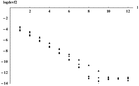
The prediction (4.4) for the finite volume two-particle form factors is compared with spin- $0$ states graphically in figure 4.8 and numerically in table 4.2, while the spin- $1$ and spin- $2$ case is presented in figure 4.9 and in table 4.3. These contain no more than a representative sample of our data: we evaluated similar matrix elements for a large number of two-particle states for values of the volume parameter $l$ running from $1$ to $30$ . The behaviour of the relative deviation is consistent with the presence of a correction of $e^{-l}$ type up to $l\sim 9\dots 10$ (i.e. the logarithm of the deviation is very close to being a linear function of $l$ ), and after $l\sim 16\dots 18$ it starts to increase due to truncation errors. This is demonstrated in figure 4.10 using the data presented in table 4.3 for spin- $1$ and spin- $2$ states²² 2 Note that the dependence of the logarithm of the deviation on the volume is not exactly linear because the residual finite size correction can also contain a factor of some power of $l$ , and so it is expected that a $\log l$ contribution is also present in the data plotted in figure 4.10., but it is equally valid for all the other states we examined. In the intermediate region $l\sim 10\dots 16$ the two sources of numerical deviation are of the same order, and so that range can be considered as the optimal scaling region: according to the data in the tables agreement there is typically around $10^{-4}$ (relative deviation). It is also apparent that scaling behaviour starts at quite low values of the volume (around $l\sim 4$ the relative deviation is already down to around 1%).

It can be verified by explicit evaluation that in the scaling region the Bethe-Yang density of states ( $\rho$ ) given in (2.17) differs by corrections of relative magnitude $10^{-1}-10^{-2}$ (analytically: of order $1/l$ ) from the free density of states ( $\rho^{0}$ ) in (2.13), and therefore without using the proper interacting density of states it is impossible to obtain the precision agreement we demonstrated. In fact the observed $10^{-4}$ relative deviation corresponds to corrections of order $l^{-4}$ at $l=10$ , but it is of the order of estimated truncation errors³³ 3 Truncation errors can be estimated by examining the dependence of the extracted data on the cutoff $e_{\mathrm{cut}}$ , as well as by comparing TCSA energy levels to the Bethe-Yang predictions..

These results are very strong evidence for the main statement in (4.4) (and thus also (2.16)), namely, that all $1/L$ corrections are accounted by the proper interacting state density factor and that all further finite size corrections are just residual finite size effects decaying exponentially in $L$ . In section 4.3 we show that data from higher multi-particle form factors fully support the above conclusions drawn from the two-particle form factors.

	$I_{1}=1/2$ , $I_{2}=-1/2$		$I_{1}=3/2$ , $I_{2}=-3/2$		$I_{1}=5/2$ , $I_{2}=-5/2$
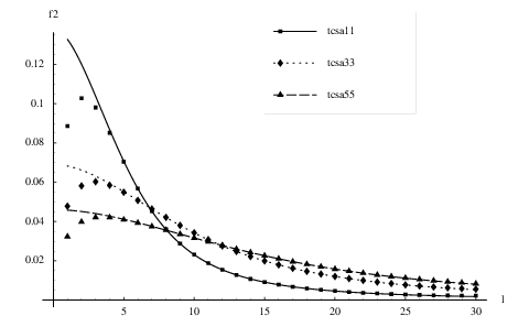
$l$	TCSA	FF	TCSA	FF	TCSA	FF
2	0.102780	0.120117	0.058158	0.066173	0.039816	0.045118
4	0.085174	0.086763	0.058468	0.059355	0.042072	0.042729
6	0.056828	0.056769	0.050750	0.050805	0.039349	0.039419
8	0.036058	0.035985	0.042123	0.042117	0.035608	0.035614
10	0.023168	0.023146	0.034252	0.034248	0.031665	0.031664
12	0.015468	0.015463	0.027606	0.027604	0.027830	0.027828
14	0.010801	0.010800	0.022228	0.022225	0.024271	0.024267
16	0.007869	0.007867	0.017976	0.017972	0.021074	0.021068
18	0.005950	0.005945	0.014652	0.014645	0.018268	0.018258
20	0.004643	0.004634	0.012061	0.012050	0.015844	0.015827

Table 4.2: Two-particle form factors

\left|f_{2}(l)\right|

in the spin-

0

sector

	$I_{1}=3/2$ , $I_{2}=-1/2$		$I_{1}=5/2$ , $I_{2}=-3/2$		$I_{1}=5/2$ , $I_{2}=-1/2$		$I_{1}=7/2$ , $I_{2}=-3/2$
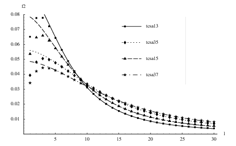
$l$	TCSA	FF	TCSA	FF	TCSA	FF	TCSA	FF
2	0.077674	0.089849	0.048170	0.054711	0.064623	0.074763	0.042031	0.047672
4	0.072104	0.073571	0.049790	0.050566	0.062533	0.063932	0.044034	0.044716
6	0.056316	0.056444	0.045031	0.045100	0.051828	0.052009	0.040659	0.040724
8	0.042051	0.042054	0.039191	0.039193	0.041370	0.041394	0.036284	0.036287
10	0.031146	0.031144	0.033469	0.033467	0.032757	0.032759	0.031850	0.031849
12	0.023247	0.023245	0.028281	0.028279	0.026005	0.026004	0.027687	0.027684
14	0.017619	0.017616	0.023780	0.023777	0.020802	0.020799	0.023941	0.023936
16	0.013604	0.013599	0.019982	0.019977	0.016808	0.016802	0.020659	0.020652
18	0.010717	0.010702	0.016831	0.016822	0.013735	0.013724	0.017835	0.017824
20	0.008658	0.008580	0.014249	0.014227	0.011357	0.011337	0.015432	0.015413

Table 4.3: Two-particle form factors

\left|f_{2}(l)\right|

in the spin-

1

and spin-

2

sectors

4.2.2 Ising model in magnetic field

In this case, there is some further subtlety to be solved before proceeding to the numerical comparison. Namely, there are spin- $0$ states which are parity reflections of each other, but are degenerate according to the Bethe-Yang equations. An example is the state $|\{1,-1\}\rangle_{12}$ in figure 4.11 (b), which is degenerate with $|\{-1,1\}\rangle_{12}$ to all orders in $1/L$ . In general the degeneracy of these states is lifted by residual finite size effects (more precisely by quantum mechanical tunneling – a detailed discussion of this mechanism was given in the framework of the $k$ -folded sine-Gordon model in [41]). Since the finite volume spectrum is parity symmetric, the TCSA eigenvectors correspond to the states

|\{1,-1\}\rangle_{12,\,L}^{\pm}=\frac{1}{\sqrt{2}}\left(|\{1,-1\}\rangle_{12,\,L}\pm|\{-1,1\}\rangle_{12,\,L}\right)

Because the Hilbert space inner product is positive definite, the TCSA eigenvectors $|\{1,-1\}\rangle_{12}^{\pm}$ can be chosen orthonormal and the problem can be resolved by calculating the form factor matrix element using the two-particle state vectors

\frac{1}{\sqrt{2}}\left(|\{1,-1\}\rangle_{12,\,L}^{+}\pm|\{1,-1\}\rangle_{12,\,L}^{-}\right)

Because the Ising spectrum is much more complicated than that of the scaling Lee-Yang model (and truncation errors are larger as well), we only identified two-particle states containing two copies of $A_{1}$ , or an $A_{1}$ and an $A_{2}$ . The numerical results are plotted in figures 4.11 (a) and (b), respectively. The finite volume form factor functions of the operator $\Psi$ (4.3) are defined as

\bar{f}_{11}\left(l\right)_{I_{1}I_{2}}=\sqrt{\rho_{11}(\tilde{\theta}_{1}(l),\tilde{\theta}_{2}(l))}\langle 0|\Psi|\{I_{1},I_{2}\}\rangle_{11}

where

	$\displaystyle l\sinh\tilde{\theta}_{1}+\delta_{11}(\tilde{\theta}_{1}-\tilde{\theta}_{2})=2\pi I_{1}$
	$\displaystyle l\sinh\tilde{\theta}_{2}+\delta_{11}(\tilde{\theta}_{2}-\tilde{\theta}_{1})=2\pi I_{2}$
	$\displaystyle\rho_{11}(\theta_{1},\theta_{2})=l^{2}\cosh\theta_{1}\cosh\theta_{2}+l\cosh\theta_{1}\varphi_{11}(\theta_{2}-\theta_{1})+l\cosh\theta_{2}\varphi_{11}(\theta_{1}-\theta_{2})$
	$\displaystyle\varphi_{11}(\theta)=\frac{d\delta_{11}(\theta)}{d\theta}$

and

\bar{f}_{12}\left(l\right)_{I_{1}I_{2}}=\sqrt{\rho_{11}(\tilde{\theta}_{1},\tilde{\theta}_{2})}\langle 0|\Psi|\{I_{1},I_{2}\}\rangle_{12}

with

	$\displaystyle l\sinh\tilde{\theta}_{1}+\delta_{12}(\tilde{\theta}_{1}-\tilde{\theta}_{2})=2\pi I_{1}$
	$\displaystyle\frac{m_{2}}{m_{1}}l\sinh\tilde{\theta}_{2}+\delta_{12}(\tilde{\theta}_{2}-\tilde{\theta}_{1})=2\pi I_{2}$
	$\displaystyle\rho_{12}(\theta_{1},\theta_{2})=\frac{m_{2}}{m_{1}}l^{2}\cosh\theta_{1}\cosh\theta_{2}+l\cosh\theta_{1}\varphi_{12}(\theta_{2}-\theta_{1})+\frac{m_{2}}{m_{1}}l\cosh\theta_{2}\varphi_{12}(\theta_{1}-\theta_{2})$
	$\displaystyle\varphi_{12}(\theta)=\frac{d\delta_{12}(\theta)}{d\theta}$

and are compared against the form factor functions

F_{2}^{\Psi}(\tilde{\theta}_{1}(l),\tilde{\theta}_{2}(l))_{11}

and

F_{2}^{\Psi}(\tilde{\theta}_{1}(l),\tilde{\theta}_{2}(l))_{12}

respectively.

Although (as we already noted) truncation errors in the Ising model are much larger than in the Lee-Yang case, extrapolation in the cutoff improves them by an order of magnitude compared to the evaluation at the highest cutoff (in our case $30$ ). After extrapolation, deviations in the scaling region become less than $1$ % (with a minimum of around $10^{-3}$ in the $A_{1}A_{1}$ , and $10^{-4}$ in the $A_{1}A_{2}$ case), and even better for states with nonzero total spin. As noted in the previous subsection this means that the numerics is really sensitive to the dependence of the particle rapidities and state density factors on the interaction between the particles; generally the truncation errors in the extrapolated data are about two orders of magnitude smaller than the interaction corrections.

It is a general tendency that the agreement is better in the sectors with nonzero spin, and the scaling region starts at smaller values of the volume. This is easy to understand for the energy levels, since for low-lying states nonzero spin generally means higher particle momenta. The higher the momenta of the particles, the more the Bethe-Yang contributions dominate over the residual finite size effects. This is consistent with the results of Rummukainen and Gottlieb in [42] where it was found that resonance phase shifts can be more readily extracted from sectors with nonzero momentum; our data show that this observation carries over to general matrix elements as well.

4.3 Many-particle form factors

4.3.1 Scaling Lee-Yang model

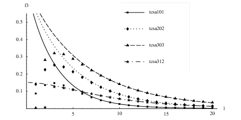
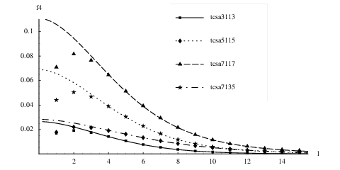
We also performed numerical evaluation of three and four-particle form factors in the scaling Lee-Yang model; some of the results are presented in figures 4.12 and 4.13, respectively. For the sake of brevity we refrain from presenting explicit numerical tables; we only mention that the agreement between the numerical TCSA data and the prediction from the exact form factor solution is always better than $10^{-3}$ in the scaling region. For better visibility we plotted the functions

\tilde{f}_{k}(l)_{I_{1}\dots I_{k}}=-im^{2/5}\sqrt{\rho_{k}(\tilde{\theta}_{1},\dots,\tilde{\theta}_{k})}\langle 0|\Phi|\{I_{1},\dots,I_{k}\}\rangle_{L}\quad,\quad l=mL

for which relation (2.16) gives:

\tilde{f}_{k}(l)_{I_{1}\dots I_{k}}=-im^{2/5}F_{k}^{\Phi}(\tilde{\theta}_{1},\dots,\tilde{\theta}_{k})+O(\mathrm{e}^{-l})

(4.5)

Due to the fact that in the Lee-Yang model there is only a single particle species, we introduced the simplified notation $\rho_{n}$ for the $n$ -particle Jacobi determinant.

The complication noted in subsection 4.2.2 for the Ising state $|\{1,-1\}\rangle_{12}$ is present in the Lee-Yang model as well. The Bethe-Yang equations give degenerate energy values for the states $|\{I_{1},\dots,I_{k}\}\rangle_{L}$ and $|\{-I_{k},\dots,-I_{1}\}\rangle_{L}$ (as noted before, the degeneracy is lifted by quantum mechanical tunneling). For states with nonzero spin this causes no problem, because these two states are in sectors of different spin (their spins differ by a sign) and similarly there is no difficulty when the two quantum number sets are identical, i.e.

\{I_{1},\dots,I_{k}\}=\{-I_{1},\dots,-I_{k}\}

since then there is a single state. However, there are states in the zero spin sector (i.e. with $\sum_{k}I_{k}=0$ ) for which

\{I_{1},\dots,I_{k}\}\neq\{-I_{1},\dots,-I_{k}\}

We use two such pairs of states in our data here: the three-particle states $|\{3,-1,-2\}\rangle_{L}$ , $|\{2,1,-3\}\rangle_{L}$ and the four-particle states $|\{7/2,1/2,-3/2,-5/2\}\rangle_{L}$ , $|\{5/2,3/2,-1/2,-7/2\}\rangle_{L}$ . Again, the members of such pairs are related to each other by spatial reflection, which is a symmetry of the exact finite-volume Hamiltonian and therefore (supposing that the eigenvectors are orthonormal) the finite volume eigenstates correspond to

|\{I_{1},\dots,I_{k}\}\rangle_{L}^{\pm}=\frac{1}{\sqrt{2}}\left(|\{I_{1},\dots,I_{k}\}\rangle_{L}\pm|\{-I_{k},\dots,-I_{1}\}\rangle_{L}\right)

and this must be taken into account when evaluating the form factor matrix elements. In the Lee-Yang case, however, the inner product is not positive definite (and some nonzero vectors may have zero “length”, although this does not happen for TCSA eigenvectors, because they are orthogonal to each other and the inner product is non-degenerate), but there is a simple procedure that can be used in the general case. Suppose the two TCSA eigenvectors corresponding to such a pair are $v_{1}$ and $v_{2}$ . Then we can define their inner product matrix as

g_{ij}=v_{i}G^{(0)}v_{j}

using the TCSA inner product (3.9). The appropriate basis vectors of this two-dimensional subspace, which can be identified with $|\{I_{1},\dots,I_{k}\}\rangle_{L}$ and $|\{-I_{k},\dots,-I_{1}\}\rangle_{L}$ , can be found by solving the two-dimensional generalized eigenvalue problem

g\cdot w=\lambda P\cdot w

for the vector $(w_{1},w_{2})$ describing orientation in the subspace, with

P=\left(\begin{array}[]{cc}0&1\\ 1&0\end{array}\right)

This procedure has the effect of rotating from the basis of parity eigenvectors to basis vectors which are taken into each other by spatial reflection.

4.3.2 Ising model in a magnetic field

As we already noted, it is much harder to identify⁴⁴ 4 To identify $A_{1}A_{1}A_{1}$ states it is necessary to use at least $e_{\mathrm{cut}}=22$ or $24$ and even then the agreement with the Bethe-Yang prediction is still only within $20\%$ , but the identification can be made for the first few $A_{1}A_{1}A_{1}$ states using data up to $e_{\mathrm{cut}}=30$ . Truncation errors are substantially decreased by extrapolation to $e_{\mathrm{cut}}=\infty$ . higher states in the Ising model due to the complexity of the spectrum, and so we only performed an analysis of states containing three $A_{1}$ particles. We define

\tilde{f}_{111}\left(l\right)_{I_{1}I_{2}I_{3}}=\sqrt{\rho_{111}(\tilde{\theta}_{1}(l),\tilde{\theta}_{2}(l),\tilde{\theta}_{3}(l))}\langle 0|\Psi|\{I_{1},I_{2},I_{3}\}\rangle_{111}

where $\tilde{\theta}_{i}(l)$ are the solutions of the three-particle Bethe-Yang equations in (dimensionless) volume $l$ and $\rho_{111}$ is the appropriate $3$ -particle determinant. The results of the comparison can be seen in figure 4.14. The numerical precision indicated for two-particle form factors at the end of subsection 4.2.2, as well as the remarks made there on the spin dependence apply here as well; we only wish to emphasize that for $A_{1}A_{1}A_{1}$ states with nonzero total spin the agreement between the extrapolated TCSA data and the form factor prediction in the optimal part of the scaling region is within $2\times 10^{-4}$ .

5 General form factors without disconnected pieces

Let us consider a matrix element of the form

\,{}_{j_{1}\dots j_{m}}\langle\{I_{1}^{\prime},\dots,I_{m}^{\prime}\}|\mathcal{O}(0,0)|\{I_{1},\dots,I_{n}\}\rangle_{i_{1}\dots i_{n},L}

Disconnected pieces are known to appear when there is at least one particle in the state on the left which occurs in the state on the right with exactly the same rapidity. The rapidities of particles as a function of the volume are determined by the Bethe-Yang equations (2.14)

Q_{k}(\tilde{\theta}_{1},\dots,\tilde{\theta}_{n})_{i_{1}\dots i_{n}}=m_{i_{k}}L\sinh\tilde{\theta}_{k}+\sum_{l\neq k}\delta_{i_{k}i_{l}}(\tilde{\theta}_{k}-\tilde{\theta}_{l})=2\pi I_{k}\quad,\quad k=1,\dots,n

and

Q_{k}(\tilde{\theta}_{1}^{\prime},\dots,\tilde{\theta}_{m}^{\prime})_{j_{1}\dots j_{m}}=m_{j_{k}}L\sinh\tilde{\theta}_{k}^{\prime}+\sum_{l\neq k}\delta_{j_{k}j_{l}}(\tilde{\theta}_{k}^{\prime}-\tilde{\theta}_{l}^{\prime})=2\pi I_{k}^{\prime}\quad,\quad k=1,\dots,m

Due to the presence of the scattering terms containing the phase shift functions $\delta$ , equality of two quantum numbers $I_{k}$ and $I_{l}^{\prime}$ does not mean that the two rapidities themselves are equal in finite volume $L$ . It is easy to see that there are only two cases when exact equality of some rapidities can occur:

The two states are identical, i.e. $n=m$ and

	$\displaystyle\{j_{1}\dots j_{m}\}$	$\displaystyle=$	$\displaystyle\{i_{1}\dots i_{n}\}$
	$\displaystyle\{I_{1}^{\prime},\dots,I_{m}^{\prime}\}$	$\displaystyle=$	$\displaystyle\{I_{1},\dots,I_{n}\}$

in which case all the rapidities are pairwise equal, or

Both states are parity symmetric states in the spin zero sector, i.e.

	$\displaystyle\{I_{1},\dots,I_{n}\}$	$\displaystyle\equiv$	$\displaystyle\{-I_{n},\dots,-I_{1}\}$
	$\displaystyle\{I_{1}^{\prime},\dots,I^{\prime}_{m}\}$	$\displaystyle\equiv$	$\displaystyle\{-I^{\prime}_{m},\dots,-I^{\prime}_{1}\}$

and the particle species labels are also compatible with the symmetry, i.e. $i_{n+1-k}=i_{k}$ and $j_{m+1-k}=j_{k}$ . Furthermore, both states must contain one (or possibly more, in a theory with more than one species) particle of quantum number $0$ , whose rapidity is then exactly $0$ for any value of the volume $L$ due to the symmetric assignment of quantum numbers.

Discussion of such matrix elements raises many interesting theoretical considerations and is postponed to the followup paper [20]; here we only concentrate on matrix elements for which there are no disconnected contributions.

5.1 Scaling Lee-Yang model

In this model there is a single particle species, so we can introduce the following notations:

f_{kn}(l)_{I_{1},\dots,I_{n}}^{I_{1}^{\prime},\dots,I_{k}^{\prime}}=-im^{2/5}\langle\{I_{1}^{\prime},\dots,I_{k}^{\prime}\}|\Phi(0,0)|\{I_{1},\dots,I_{n}\}\rangle_{L}

and also

\tilde{f}_{kn}(l)_{I_{1},\dots,I_{n}}^{I_{1}^{\prime},\dots,I_{k}^{\prime}}=-im^{2/5}\sqrt{\rho_{k}(\tilde{\theta}_{1}^{\prime},\dots,\tilde{\theta}_{k}^{\prime})}\sqrt{\rho_{n}(\tilde{\theta}_{1},\dots,\tilde{\theta}_{n})}\langle\{I_{1}^{\prime},\dots,I_{k}^{\prime}\}|\Phi(0,0)|\{I_{1},\dots,I_{n}\}\rangle_{L}

for which relation (2.20) yields

	$\displaystyle f_{kn}(l)_{I_{1},\dots,I_{n}}^{I_{1}^{\prime},\dots,I_{k}^{\prime}}$	$\displaystyle=$	$\displaystyle-im^{2/5}\frac{F_{k+n}^{\Phi}(\tilde{\theta}_{k}^{\prime}+i\pi,\dots,\tilde{\theta}_{1}^{\prime}+i\pi,\tilde{\theta}_{1},\dots,\tilde{\theta}_{n})}{\sqrt{\rho_{n}(\tilde{\theta}_{1},\dots,\tilde{\theta}_{n})\rho_{k}(\tilde{\theta}_{1}^{\prime},\dots,\tilde{\theta}_{m}^{\prime})}}+O(\mathrm{e}^{-l})$
	$\displaystyle\tilde{f}_{kn}(l)_{I_{1},\dots,I_{n}}^{I_{1}^{\prime},\dots,I_{k}^{\prime}}$	$\displaystyle=$	$\displaystyle-im^{2/5}F_{k+n}^{\Phi}(\tilde{\theta}_{k}^{\prime}+i\pi,\dots,\tilde{\theta}_{1}^{\prime}+i\pi,\tilde{\theta}_{1},\dots,\tilde{\theta}_{n})+O(\mathrm{e}^{-l})$		(5.1)

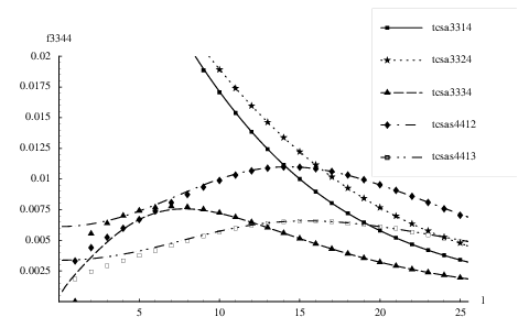
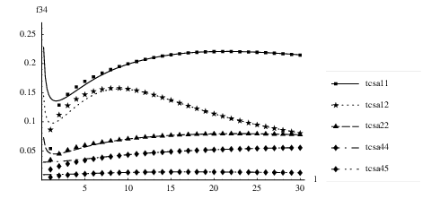
For the plots we chose to display $f$ or $\tilde{f}$ depending on which one gives a better visual picture. The numerical results shown here are just a fraction of the ones we actually obtained, but all of them show an agreement with precision $10^{-4}-10^{-3}$ in the scaling region (the volume range corresponding to the scaling region typically varies depending on the matrix element considered due to variation in the residual finite size corrections and truncation effects).

The simplest cases involve one and two-particle states: the one-particle–one-particle data in figure 5.1 actually test the two-particle form factor $F_{2}^{\Phi}$ , while the one-particle–two-particle plot 5.2 corresponds to $F_{3}^{\Phi}$ (we obtained similar results on $F_{4}^{\Phi}$ using matrix elements $f_{22}$ ). Note that in contrast to the comparisons performed in subsections 4.2 and 4.3, these cases involve the form factor solutions (3.12) at complex values of the rapidities. In general, all tests performed with TCSA can test form factors at rapidity arguments with imaginary parts $0$ or $\pi$ , which are the only parts of the complex rapidity plane where form factors eventually correspond to physical matrix elements.

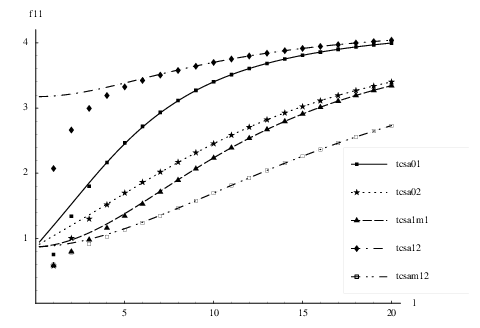
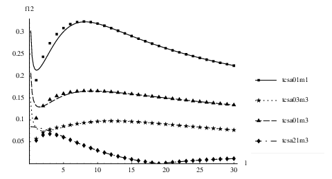
One-particle–three-particle and one-particle–four-particle matrix elements $f_{13}$ and $f_{14}$ contribute another piece of useful information. We recall that there are pairs of parity-related states in the spin-0 factors which we cannot distinguish in terms of their elementary form factors. In subsection 4.3 we showed the example of the three-particle states

|\{3,-1,-2\}\rangle_{L}\mbox{ and }|\{2,1,-3\}\rangle_{L}

and the four-particle states

|\{7/2,1/2,-3/2,-5/2\}\rangle_{L}\mbox{ and }|\{5/2,3/2,-1/2,-7/2\}\rangle_{L}

In fact it is only true that they cannot be distinguished if the left state is parity-invariant. However, using a one-particle state of nonzero spin on the left it is possible to distinguish and appropriately label the two states, as shown in figures 5.3 and 5.4. This can also be done using matrix elements with two-particle states of nonzero spin: the two-particle–three-particle case $f_{23}$ is shown in 5.5 (similar results were obtained for $f_{24}$ ). Examining the data in detail shows that the identifications provided using different states on the left are all consistent with each other.

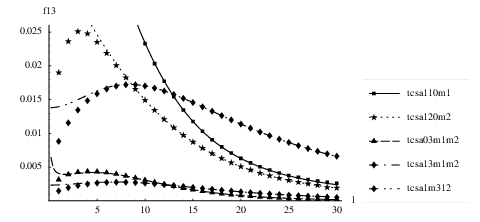
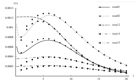
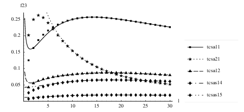
It is also interesting to note that the $f_{14}$ (figure 5.4) and $f_{23}$ data (figure 5.5) provide a test for the five-particle form factor solutions $F_{5}$ . This is important since it is progressively harder to identify many-particle states in the TCSA spectrum for two reasons. First, the spectrum itself becomes more and more dense as we look for higher levels; second, the truncation errors grow as well. Both of these make the identification of the energy levels by comparison with the predictions of the Bethe-Yang equations more difficult; in the Lee-Yang case we stopped at four-particle levels. However, using general matrix elements and the relations (5.1) we can even get data for form factors up to $8$ particles, a sample of which is shown in figures 5.6 ( $f_{33}$ and $f_{44}$ , corresponding to $6$ and $8$ particle form-factors) and 5.7 ( $f_{34}$ which corresponds to $7$ particle form factors).

5.2 Ising model in magnetic field

In the case of the Ising model, we define the functions

\tilde{f}_{j_{1}\dots j_{m};i_{1}\dots i_{n}}(l)=\sqrt{\rho_{i_{1}\dots i_{n}}(\tilde{\theta}_{1},\dots,\tilde{\theta}_{n})\rho_{j_{1}\dots j_{m}}(\tilde{\theta}_{1}^{\prime},\dots,\tilde{\theta}_{m}^{\prime})}\times\,_{j_{1}\dots j_{m}}\langle\{I_{1}^{\prime},\dots,I_{m}^{\prime}\}|\Psi|\{I_{1},\dots,I_{n}\}\rangle_{i_{1}\dots i_{n},L}

which are compared against form factors

F_{m+n}^{\Psi}(\tilde{\theta}_{m}^{\prime}+i\pi,\dots,\tilde{\theta}_{1}^{\prime}+i\pi,\tilde{\theta}_{1},\dots,\tilde{\theta}_{n})_{j_{m}\dots j_{1}i_{1}\dots i_{n}}

where $\tilde{\theta}_{i}$ and $\tilde{\theta}_{j}^{\prime}$ denote the rapidities obtained as solutions of the appropriate Bethe-Yang equations at the given value of the volume. We chose states for which the necessary form factor solution was already known (and given in [37]) i.e. we did not construct new form factor solutions ourselves.

One-particle–one-particle form factors are shown in figure 5.8; these provide another numerical test for the two-particle form factors examined previously in subsection 4.2.2. One-particle–two-particle form factors, besides testing again the three-particle form factor $A_{1}A_{1}A_{1}$ (figure 5.9 (a)) also provide information on $A_{1}A_{1}A_{2}$ (figure 5.9 (b)).

Finally, one-particle–three-particle and two-particle–two-particle matrix elements can be compared to the $A_{1}A_{1}A_{1}A_{1}$ form factor, which again shows that by considering general matrix elements we can go substantially higher in the form factor tree than using only elementary form factors.

We remark that the cusps on the horizontal axis in the form factor plots correspond to zeros where the form factors change sign; they are artifacts introduced by taking the absolute value of the matrix elements. The pattern of numerical deviations between TCSA data and exact form factor predictions is fully consistent with the discussion in the closing paragraphs of subsections 4.2.2 and 4.3.2. The deviations in the scaling region are around $1$ % on average, with agreement of the order of $10^{-3}$ in the optimal range.

6 Conclusions

In this work we gave an expression for the matrix elements of local operators between general multi-particle states in finite volume which is valid to any order in the expansion in the inverse of the volume $1/L$ . It was shown in section 2.2 using a very general argument that all the remaining volume dependence is non-analytic in $1/L$ (it is given by residual finite size effects vanishing exponentially with increasing volume). It is also clear that the derivation itself does not depend on integrability, neither it is restricted to $1+1$ dimensional field theories and therefore relations (2.16) and (2.20) can be extended to general quantum field theories (substituting the rapidities with appropriate kinematical parametrization and the $\rho_{n}$ with the proper state densities), with the only condition that their spectrum of excitations must possess a mass gap.

$1+1$ dimensional integrable field theories are special in the respect that multi-particle states in finite volume can be described using the Bethe-Yang equations (2.14) and so the $n$ -particle state density $\rho_{n}$ can be obtained in the general closed form (2.17). Another important feature is that there are exact results for matrix elements of local operators in infinite volume which can be obtained from the form factor bootstrap briefly reviewed in section 2.1. Therefore they are ideal toy models to test ideas about finite size corrections. Such an approach is also interesting due to a fundamental property of the bootstrap, namely that it is only indirectly related to the actual Lagrangian (or Hamiltonian) field theory. As we discussed in the introduction, testing the conjectured form factors against field theory usually involves calculating two-point functions using spectral representations, or sum rules derived from such expansions; however, direct non-perturbative comparison of the actual form factors to matrix elements computed from the field theory have been very restricted so far.

Using TCSA we were able to give an extensive and direct numerical comparison between bootstrap results for form factors and matrix elements evaluated non-perturbatively. One of the advantages is that we can compare matrix elements directly, without using any proxy (such as a two-point function or a sum rule); the other is the very high precision of the comparison and also that it is possible to test form factors of many particles which have never been tested using spectral sums, mostly due to the fact that usually their contribution to spectral expansions is extremely small, and evaluating it also involves calculating multidimensional integrals to very high precision, which a numerically difficult task. The second problem is actually related to the first, since due to the smallness of the contribution from higher particle terms all the lower ones must be evaluated to sufficiently high precision. Our approach, in contrast, makes it possible to have a test of entire one-dimensional sections of the form factor functions using the volume as a parameter, and the number of available sections only depends on our ability to identify multi-particle states in finite volume.

Our results can also be viewed in the context of finite volume form factors [15] (which is also related to the problem of finite temperature form factors; for a review on the latter see [16] and references therein). The relations (2.16, 2.20) give finite volume form factors expressed with their infinite volume counterparts to all orders in $1/L$ (where $L$ denotes the volume), i.e. up to exponentially decaying terms in $L$ . This gives finite volume form factors in large volume with very high precision. On the other hand, what we determine numerically in TCSA are actually the finite volume form factors themselves, which is an approach that primarily works in small enough volume due to the truncation errors. In the Lee-Yang case, the combination of the two approaches gives the finite volume form factors involving up to four particles with better than $10^{-3}$ relative precision, as demonstrated by the excellent agreement in the scaling region of TCSA where their domains of validity overlap. For the Ising model the numerical precision is not as good, but with some care a precision of around $10^{-3}$ can be achieved for most of the matrix elements considered in this paper.

An open question which is not discussed in this paper is the case of matrix elements with disconnected pieces. Results on such matrix elements are already available, but we postpone them to a followup paper [20] where we also plan to discuss many theoretical issues related to crossing and disconnected contributions in finite volume.

Acknowledgments

We wish to thank Z. Bajnok and L. Palla for useful discussions. This research was partially supported by the Hungarian research funds OTKA T043582, K60040 and TS044839. GT was also supported by a Bolyai János research scholarship.

References

[1] A.B. Zamolodchikov and Al.B. Zamolodchikov, Annals Phys. 120 (1979) 253-291.
[2] G. Mussardo, Phys. Rept. 218 (1992) 215-379.
[3] M. Karowski and P. Weisz, Nucl. Phys. B139 (1978) 455.
B. Berg, M. Karowski and P. Weisz, Phys. Rev. D19 (1979) 2477.
M. Karowski, Phys. Rep. 49 (1979) 229.
[4] F.A. Smirnov: Form-factors in completely integrable models of quantum field theory, Adv. Ser. Math. Phys. 14 (1992) 1-208.
[5] J.L. Cardy and G. Mussardo, Nucl. Phys. B340 (1990) 387-402.
[6] A. Koubek and G. Mussardo, Phys. Lett. B311 (1993) 193-201, hep-th/9306044.
[7] A. Koubek, Nucl. Phys. B428 (1994) 655-680, hep-th/9405014.
[8] A. Koubek, Nucl. Phys. B435 (1995) 703-734, hep-th/9501029.
[9] F.A. Smirnov, Nucl. Phys. B453 (1995) 807-824, hep-th/9501059.
[10] V.P. Yurov and Al.B. Zamolodchikov, Int. J. Mod. Phys. A6 (1991) 3419-3440.
[11] Al.B. Zamolodchikov, Nucl. Phys. B348 (1991) 619-641.
[12] A.B. Zamolodchikov, Pis’ma Zh Eksp. Theor. Fiz. 43 (1986) 565. (JETP Lett. 43 (1986) 730.)
[13] J.L. Cardy, Phys. Rev. Lett. 60 (1988) 2709.
A. Cappelli, D. Friedan and J.I. Latorre, Nucl. Phys. B352 (1991) 616-670.
D.Z. Freedman, J.I. Latorre and X. Vilasis, Mod. Phys. Lett. A6 (1991) 531-542.
[14] G. Delfino, P. Simonetti and J.L. Cardy, Phys. Lett. B387 (1996) 327-333, hep-th/9607046.
[15] F.A. Smirnov, hep-th/9802132.
V.E. Korepin and N.A. Slavnov, Int. J. Mod. Phys. B13 (1999) 2933-2942, math-ph/9812026.
G. Mussardo, V. Riva, and G. Sotkov, Nucl. Phys. B670 (2003) 464-578, hep-th/0307125.
[16] B. Doyon, SIGMA 3 (2007) 011, hep-th/0611066.
[17] G. Takács and B. Pozsgay, Nucl. Phys. B748 (2006) 485-523, hep-th/0604022.
[18] V.P. Yurov and Al.B. Zamolodchikov, Int. J. Mod. Phys. A5 (1990) 3221-3246.
[19] L. Lellouch and M. Lüscher, Commun. Math. Phys. 219 (2001) 31-44, hep-lat/0003023.
[20] B. Pozsgay and G. Takács: Form factors in finite volume II: disconnected terms and finite temperature correlators, arXiv: 0706.3605 [hep-th].
[21] M. Lüscher, Commun. Math. Phys. 104 (1986) 177.
[22] T.R. Klassen and E. Melzer, Nucl. Phys. B362 (1991) 329-388.
[23] M. Lüscher, Comm. Math. Phys. 105 (1986) 153-188.
[24] G. Delfino and G. Mussardo, Nucl. Phys. B455 (1995) 724-758, hep-th/9507010.
[25] C.J.D. Lin, G. Martinelli, C.T. Sachrajda and M. Testa, Nucl. Phys. B619 (2001) 467-498, hep-lat/0104006.
[26] B. Pozsgay, work in progress.
[27] H. Saleur, Nucl. Phys. B567 (2000) 602-610, hep-th/9909019.
[28] Al.B. Zamolodchikov, Nucl. Phys. B342 (1990) 695-720.
[29] J.L. Cardy and G. Mussardo, Phys. Lett. B225 (1989) 275-278.
[30] H. Kausch, G. Takács and G. Watts, Nucl. Phys. B489 (1997) 557-579, hep-th/9605104.
[31] A.B. Zamolodchikov, Advanced Studies in Pure Mathematics 19 (1989) 641; Int. J. Mod. Phys. A3 (1988) 743.
[32] V.A. Fateev, Phys. Lett. B324 (1994) 45-51.
[33] V. P. Yurov and Al.B. Zamolodchikov, Int. J. Mod. Phys. A6 (1991) 4557-4578.
[34] G. Delfino and P. Simonetti, Phys. Lett. B383 (1996) 450-456, hep-th/9605065.
[35] G. Delfino, P. Grinza and G. Mussardo, Nucl. Phys. B737 (2006) 291-303, hep-th/0507133.
[36] V.A. Fateev, S. Lukyanov, A.B. Zamolodchikov and Al.B. Zamolodchikov, Nucl. Phys. B516 (1998) 652-674, hep-th/9709034.
[37] http://people.sissa.it/~delfino/isingff.html
[38] R. Guida and N. Magnoli, Phys. Lett. B411 (1997) 127-133, hep-th/9706017.
[39] D. Fioravanti, G. Mussardo and P. Simon, Phys. Rev. E63 (2001) 016103, cond-mat/0008216.
[40] G. Delfino, J. Phys. A34 (2001) L161-L168, hep-th/0101180.
[41] Z. Bajnok, L. Palla, G. Takács and F. Wágner, Nucl. Phys. B587 (2000) 585-618, hep-th/0004181.
[42] K. Rummukainen and S.A. Gottlieb, Nucl. Phys. B450 (1995) 397-436, hep-lat/9503028.

	$\displaystyle F_{mn}^{\mathcal{O}}(\theta_{1}^{{}^{\prime}},\dots,\theta_{m}^{{}^{\prime}}\|\theta_{1},\dots,\theta_{n})_{j_{1}\dots j_{m};i_{1}\dots i_{n}}=$
	$\displaystyle\qquad F_{m-1n+1}^{\mathcal{O}}(\theta_{1}^{{}^{\prime}},\dots,\theta_{m-1}^{{}^{\prime}}\|\theta_{m}^{{}^{\prime}}+i\pi,\theta_{1},\dots,\theta_{n})_{j_{1}\dots j_{m-1};j_{m}i_{1}\dots i_{n}}$
	$\displaystyle\qquad+\sum_{k=1}^{n}\Big(2\pi\delta_{j_{m}i_{k}}\delta(\theta_{m}^{{}^{\prime}}-\theta_{k})\prod_{l=1}^{k-1}S_{i_{l}i_{k}}(\theta_{l}-\theta_{k})\times$
	$\displaystyle\qquad F_{m-1n-1}^{\mathcal{O}}(\theta_{1}^{{}^{\prime}},\dots,\theta_{m-1}^{{}^{\prime}}\|\theta_{1},\dots,\theta_{k-1},\theta_{k+1}\dots,\theta_{n})_{j_{1}\dots j_{m-1};j_{m}i_{1}\dots i_{k-1}i_{k+1}\dots i_{n}}\Big)$		(2.2)

	$\displaystyle\|\{I_{1},\dots,I_{n}\}\rangle_{L}$	$\displaystyle=$	$\displaystyle\sum_{i}\Psi_{i}(I_{1},\dots,I_{n};L)\|i\rangle$
	$\displaystyle\|\{I_{1}^{\prime},\dots,I_{k}^{\prime}\}\rangle_{L}$	$\displaystyle=$	$\displaystyle\sum_{j}\Psi_{j}(I_{1}^{\prime},\dots,I_{k}^{\prime};L)\|j\rangle$

ITP-Budapest Report No. 634 Form factors in finite volume I: form factor bootstrap and truncated conformal space

Abstract

1 Introduction

2 Form factors in finite volume

2.1 Form factor bootstrap

2.2 Finite size corrections for form factors

3 Form factors from truncated conformal space

3.1 Scaling Lee-Yang model

3.1.1 Truncated conformal space approach for scaling Lee-Yang model

3.1.2 Exact form factors of the primary field Φ\Phi

3.2 Ising model with magnetic perturbation

3.2.1 Truncated fermionic space approach for the Ising model

3.2.2 Form factors of the energy density operator ϵ\epsilon

3.3 Evaluating matrix elements of a local operator 𝒪\mathcal{O} in TCSA

3.3.1 Identification of multi-particle states

3.3.2 Evaluation of matrix elements

4 Numerical results for elementary form factors

4.1 Vacuum expectation values and one-particle form factors

4.1.1 Scaling Lee-Yang model

4.1.2 Ising model in magnetic field

4.2 Two-particle form factors

4.2.1 Scaling Lee-Yang model

4.2.2 Ising model in magnetic field

4.3 Many-particle form factors

4.3.1 Scaling Lee-Yang model

4.3.2 Ising model in a magnetic field

5 General form factors without disconnected pieces

5.1 Scaling Lee-Yang model

5.2 Ising model in magnetic field

6 Conclusions

Acknowledgments

References

ITP-Budapest Report No. 634 Form factors in finite volume I:
form factor bootstrap and truncated conformal space

3.1.2 Exact form factors of the primary field $\Phi$

3.2.2 Form factors of the energy density operator $\epsilon$

3.3 Evaluating matrix elements of a local operator $\mathcal{O}$ in TCSA