Extended Theories of Gravity and their Cosmological and Astrophysical Applications
Abstract
Astrophysical observations are pointing out huge amounts of "dark matter" and "dark energy" needed to explain the observed large scale structure and cosmic dynamics. The emerging picture is a spatially flat, homogeneous Universe undergoing the today observed accelerated phase. Despite of the good quality of astrophysical surveys, commonly addressed as Precision Cosmology, the nature and the nurture of dark energy and dark matter, which should constitute the bulk of cosmological matter-energy, are still unknown. Furthermore, up to now, no experimental evidence has been found, at fundamental level, to explain such mysterious components.
The problem could be completely reversed considering dark matter and dark energy as "shortcomings" of General Relativity in its simplest formulation (a linear theory in the Ricci scalar , minimally coupled to the standard perfect fluid matter) and claiming for the "correct" theory of gravity as that derived by matching the largest number of observational data, without imposing any theory a priori. As a working hypothesis, accelerating behavior of cosmic fluid, large scale structure, potential of galaxy clusters, rotation curves of spiral galaxies could be reproduced by means of extending the standard theory of General Relativity. In other words, gravity could acts in different ways at different scales and the above "shortcomings" could be due to incorrect extrapolations of the Einstein gravity, actually tested at short scales and low energy regimes.
After a survey of what is intended for Extended Theories of Gravity in the so called "metric" and "Palatini" approaches, we discuss some cosmological and astrophysical applications where the issues related to the dark components are addressed by enlarging the Einstein theory to more general Lagrangians, where is a generic function of Ricci scalar , not assumed simply linear. Obviously, this is not the final answer to the problem of "dark-components" but it can be considered as an operative scheme whose aim is to avoid the addition of unknown exotic ingredients to the cosmic pie.
Keywords:
Extended Theories of Gravity; Dark Energy; Dark Matter; Observations.I Introduction
General Relativity (GR) is a comprehensive theory of spacetime, gravity and matter. Its formulation implies that space and time are not "absolute" entities, as in Classical Mechanics, but dynamical quantities strictly related to the distribution of matter and energy. As a consequence, this approach gave rise to a new conception of the Universe itself which, for the first time, was considered as a dynamical system. In other words, Cosmology has been enclosed in the realm of Science and not only of Philosophy, as before the Einstein work. On the other hand, the possibility of a scientific investigation of the Universe has led to the formulation of the Standard Cosmological Model weinberg which, quite nicely, has matched with observations.
Despite of these results, in the last thirty years, several shortcomings came out in the Einstein theory and people began to investigate whether GR is the only fundamental theory capable of explaining the gravitational interaction. Such issues come, essentially, from cosmology and quantum field theory. In the first case, the presence of the Big Bang singularity, the flatness and horizon problems guth led to the statement that Cosmological Standard Model, based on the GR and the Standard Model of Particle Physics, is inadequate to describe the Universe at extreme regimes. On the other hand, GR is a classical theory which does not work as a fundamental theory, when one wants to achieve a full quantum description of spacetime (and then of gravity).
Due to these facts and, first of all, to the lack of a definitive quantum gravity theory, alternative theories have been considered in order to attempt, at least, a semi-classical scheme where GR and its positive results could be recovered. One of the most fruitful approaches has been that of Extended Theories of Gravity (ETG) which have become a sort of paradigm in the study of gravitational interaction. They are based on corrections and enlargements of the Einstein theory. The paradigm consists, essentially, in adding higher-order curvature invariants and minimally or non-minimally coupled scalar fields into dynamics which come out from the effective action of quantum gravity odintsov.
Other motivations to modify GR come from the issue of a full recovering of the Mach principle which leads to assume a varying gravitational coupling. The principle states that the local inertial frame is determined by some average of the motion of distant astronomical objects bondi. This fact implies that the gravitational coupling can be scale-dependent and related to some scalar field. As a consequence, the concept of “inertia” and the Equivalence Principle have to be revised. For example, the Brans-Dicke theory brans is a serious attempt to define an alternative theory to the Einstein gravity: it takes into account a variable Newton gravitational coupling, whose dynamics is governed by a scalar field non-minimally coupled to the geometry. In such a way, Mach’s principle is better implemented brans; cimento; sciama.
Besides, every unification scheme as Superstrings, Supergravity or Grand Unified Theories, takes into account effective actions where non-minimal couplings to the geometry or higher-order terms in the curvature invariants are present. Such contributions are due to one-loop or higher-loop corrections in the high-curvature regimes near the full (not yet available) quantum gravity regime odintsov. Specifically, this scheme was adopted in order to deal with the quantization on curved spacetimes and the result was that the interactions among quantum scalar fields and background geometry or the gravitational self-interactions yield corrective terms in the Hilbert-Einstein Lagrangian birrell. Moreover, it has been realized that such corrective terms are inescapable in order to obtain the effective action of quantum gravity at scales closed to the Planck one vilkovisky. All these approaches are not the “full quantum gravity" but are needed as working schemes toward it.
In summary, higher-order terms in curvature invariants (such as , , , , or ) or non-minimally coupled terms between scalar fields and geometry (such as ) have to be added to the effective Lagrangian of gravitational field when quantum corrections are considered. For instance, one can notice that such terms occur in the effective Lagrangian of strings or in Kaluza-Klein theories, when the mechanism of dimensional reduction is used veneziano.
On the other hand, from a conceptual viewpoint, there are no a priori reason to restrict the gravitational Lagrangian to a linear function of the Ricci scalar , minimally coupled with matter francaviglia. Furthermore, the idea that there are no “exact” laws of physics could be taken into serious account: in such a case, the effective Lagrangians of physical interactions are “stochastic” functions. This feature means that the local gauge invariances (i.e. conservation laws) are well approximated only in the low energy limit and the fundamental physical constants can vary ottewill.
Besides fundamental physics motivations, all these theories have acquired a huge interest in cosmology due to the fact that they “naturally" exhibit inflationary behaviors able to overcome the shortcomings of Cosmological Standard Model (based on GR). The related cosmological models seem realistic and capable of matching with the CMBR observations starobinsky; kerner; la. Furthermore, it is possible to show that, via conformal transformations, the higher-order and non-minimally coupled terms always correspond to the Einstein gravity plus one or more than one minimally coupled scalar fields teyssandier; maeda; wands1; wands; gottloeber.
More precisely, higher-order terms appear always as contributions of order two in the field equations. For example, a term like gives fourth order equations ruzmaikin, gives sixth order equations gottloeber; sixth, gives eighth order equations eight and so on. By a conformal transformation, any 2nd-order derivative term corresponds to a scalar field11 1 The dynamics of such scalar fields is usually given by the corresponding Klein-Gordon Equation, which is second order.: for example, fourth-order gravity gives Einstein plus one scalar field, sixth-order gravity gives Einstein plus two scalar fields and so on gottloeber; schmidt1.
Furthermore, it is possible to show that the -gravity is equivalent not only to a scalar-tensor one but also to the Einstein theory plus an ideal fluid cno. This feature results very interesting if we want to obtain multiple inflationary events since an early stage could select “very” large-scale structures (clusters of galaxies today), while a late stage could select “small” large-scale structures (galaxies today) sixth. The philosophy is that each inflationary era is related to the dynamics of a scalar field. Finally, these extended schemes could naturally solve the problem of “graceful exit" bypassing the shortcomings of former inflationary models la; aclo.
In addition to the revision of Standard Cosmology at early epochs (leading to the Inflation), a new approach is necessary also at late epochs. ETGs could play a fundamental role also in this context. In fact, the increasing bulk of data that have been accumulated in the last few years have paved the way to the emergence of a new cosmological model usually referred to as the Concordance Model.
The Hubble diagram of Type Ia Supernovae (hereafter SNeIa), measured by both the Supernova Cosmology Project SCP and the High - z Team HZT up to redshift , has been the first evidence that the Universe is undergoing a phase of accelerated expansion. On the other hand, balloon born experiments, such as BOOMERanG Boomerang and MAXIMA Maxima, determined the location of the first and second peak in the anisotropy spectrum of the cosmic microwave background radiation (CMBR) strongly pointing out that the geometry of the Universe is spatially flat. If combined with constraints coming from galaxy clusters on the matter density parameter , these data indicate that the Universe is dominated by a non-clustered fluid with negative pressure, generically dubbed dark energy, which is able to drive the accelerated expansion. This picture has been further strengthened by the recent precise measurements of the CMBR spectrum, due to the WMAP experiment WMAP; hinshaw; hinshaw1, and by the extension of the SNeIa Hubble diagram to redshifts higher than 1 Riess04.
After these observational evidences, an overwhelming flood of papers has appeared: they present a great variety of models trying to explain this phenomenon. In any case, the simplest explanation is claiming for the well known cosmological constant LCDMrev. Although it is the best fit to most of the available astrophysical data WMAP, the CDM model fails in explaining why the inferred value of is so tiny (120 orders of magnitude lower!) if compared with the typical vacuum energy values predicted by particle physics and why its energy density is today comparable to the matter density (the so called coincidence problem).
As a tentative solution, many authors have replaced the cosmological constant with a scalar field rolling down its potential and giving rise to the model now referred to as quintessence QuintRev; tsu1. Even if successful in fitting the data, the quintessence approach to dark energy is still plagued by the coincidence problem since the dark energy and matter densities evolve differently and reach comparable values for a very limited portion of the Universe evolution coinciding at present era. To be more precise, the quintessence dark energy is tracking matter and evolves in the same way for a long time. But then, at late time, somehow it has to change its behavior into no longer tracking the dark matter but starting to dominate as a cosmological constant. This is the coincidence problem of quintessence.
Moreover, it is not clear where this scalar field originates from, thus leaving a great uncertainty on the choice of the scalar field potential. The subtle and elusive nature of dark energy has led many authors to look for completely different scenarios able to give a quintessential behavior without the need of exotic components. To this aim, it is worth stressing that the acceleration of the Universe only claims for a negative pressure dominant component, but does not tell anything about the nature and the number of cosmic fluids filling the Universe.
This consideration suggests that it could be possible to explain the accelerated expansion by introducing a single cosmic fluid with an equation of state causing it to act like dark matter at high densities and dark energy at low densities. An attractive feature of these models, usually referred to as Unified Dark Energy (UDE) or Unified Dark Matter (UDM) models, is that such an approach naturally solves, al least phenomenologically, the coincidence problem. Some interesting examples are the generalized Chaplygin gas Chaplygin, the tachyon field tachyon and the condensate cosmology Bassett. A different class of UDE models has been proposed Hobbit where a single fluid is considered: its energy density scales with the redshift in such a way that the radiation dominated era, the matter era and the accelerating phase can be naturally achieved. It is worth noticing that such class of models are extremely versatile since they can be interpreted both in the framework of UDE models and as a two-fluid scenario with dark matter and scalar field dark energy. The main ingredient of the approach is that a generalized equation of state can be always obtained and observational data can be fitted.
Actually, there is still a different way to face the problem of cosmic acceleration. As stressed in LSS03, it is possible that the observed acceleration is not the manifestation of another ingredient in the cosmic pie, but rather the first signal of a breakdown of our understanding of the laws of gravitation (in the infra-red limit).
From this point of view, it is thus tempting to modify the Friedmann equations to see whether it is possible to fit the astrophysical data with models comprising only the standard matter. Interesting examples of this kind are the Cardassian expansion Cardassian and the DGP gravity DGP. Moving in this same framework, it is possible to find alternative schemes where a quintessential behavior is obtained by taking into account effective models coming from fundamental physics giving rise to generalized or higher-order gravity actions curvature (for a comprehensive review see odinoj).
For instance, a cosmological constant term may be recovered as a consequence of a non - vanishing torsion field thus leading to a model which is consistent with both SNeIa Hubble diagram and Sunyaev - Zel’dovich data coming from clusters of galaxies torsion. SNeIa data could also be efficiently fitted including higher-order curvature invariants in the gravity Lagrangian curvfit; camfr; odgauss; camfrgauss. It is worth noticing that these alternative models provide naturally a cosmological component with negative pressure whose origin is related to the geometry of the Universe thus overcoming the problems linked to the physical significance of the scalar field.
It is evident, from this short overview, the high number of cosmological models which are viable candidates to explain the observed accelerated expansion. This abundance of models is, from one hand, the signal of the fact that we have a limited number of cosmological tests to discriminate among rival theories, and, from the other hand, that a urgent degeneracy problem has to be faced. To this aim, it is useful to remark that both the SNeIa Hubble diagram and the angular size - redshift relation of compact radio sources AngTest are distance based methods to probe cosmological models so then systematic errors and biases could be iterated. From this point of view, it is interesting to search for tests based on time-dependent observables.
For example, one can take into account the lookback time to distant objects since this quantity can discriminate among different cosmological models. The lookback time is observationally estimated as the difference between the present day age of the Universe and the age of a given object at redshift . Such an estimate is possible if the object is a galaxy observed in more than one photometric band since its color is determined by its age as a consequence of stellar evolution. It is thus possible to get an estimate of the galaxy age by measuring its magnitude in different bands and then using stellar evolutionary codes to choose the model that reproduces the observed colors at best.
Coming to the weak-field-limit approximation, which essentially means considering Solar System scales, ETGs are expected to reproduce GR which, in any case, is firmly tested only in this limit will. This fact is matter of debate since several relativistic theories do not reproduce exactly the Einstein results in the Newtonian approximation but, in some sense, generalize them. As it was firstly noticed by Stelle stelle, a -theory gives rise to Yukawa-like corrections in the Newtonian potential. Such a feature could have interesting physical consequences. For example, some authors claim to explain the flat rotation curves of galaxies by using such terms sanders. Others mannheim have shown that a conformal theory of gravity is nothing else but a fourth-order theory containing such terms in the Newtonian limit. Besides, indications of an apparent, anomalous, long-range acceleration revealed from the data analysis of Pioneer 10/11, Galileo, and Ulysses spacecrafts could be framed in a general theoretical scheme by taking corrections to the Newtonian potential into account anderson; bertolami.
In general, any relativistic theory of gravitation yields corrections to the Newton potential (see for example schmidt) which, in the post-Newtonian (PPN) formalism, could be a test for the same theory will. Furthermore the newborn gravitational lensing astronomy ehlers is giving rise to additional tests of gravity over small, large, and very large scales which soon will provide direct measurements for the variation of the Newton coupling krauss, the potential of galaxies, clusters of galaxies and several other features of self-gravitating systems.
Such data will be, very likely, capable of confirming or ruling out the physical consistency of GR or of any ETG. In summary, the general features of ETGs are that the Einstein field equations result to be modified in two senses: geometry can be non-minimally coupled to some scalar field, and/or higher than second order derivative terms in the metric come out. In the former case, we generically deal with scalar-tensor theories of gravity; in the latter, we deal with higher-order theories. However combinations of non-minimally coupled and higher-order terms can emerge as contributions in effective Lagrangians. In this case, we deal with higher-order-scalar-tensor theories of gravity.
Considering a mathematical viewpoint, the problem of reducing more general theories to Einstein standard form has been extensively treated; one can see that, through a “Legendre” transformation on the metric, higher-order theories, under suitable regularity conditions on the Lagrangian, take the form of the Einstein one in which a scalar field (or more than one) is the source of the gravitational field (see for example francaviglia; sokolowski; ordsup; magnano-soko); on the other side, as discussed above, it has been studied the mathematical equivalence between models with variable gravitational coupling with the Einstein standard gravity through suitable conformal transformations (see dicke; nmc).
In any case, the debate on the physical meaning of conformal transformations is far to be solved [see faraoni and references therein for a comprehensive review]. Several authors claim for a true physical difference between Jordan frame (higher-order theories and/or variable gravitational coupling) since there are experimental and observational evidences which point out that the Jordan frame could be suitable to better match solutions with data. Others state that the true physical frame is the Einstein one according to the energy theorems magnano-soko. However, the discussion is open and no definitive statement has been formulated up to now.
The problem should be faced from a more general viewpoint and the Palatini approach to gravity could be useful to this goal. The Palatini approach in gravitational theories was firstly introduced and analyzed by Einstein himself palaeinstein. It was, however, called the Palatini approach as a consequence of an historical misunderstanding buchdahl; frafe.
The fundamental idea of the Palatini formalism is to consider the (usually torsion-less) connection , entering the definition of the Ricci tensor, to be independent of the metric defined on the spacetime . The Palatini formulation for the standard Hilbert-Einstein theory results to be equivalent to the purely metric theory: this follows from the fact that the field equations for the connection , firstly considered to be independent of the metric, give the Levi-Civita connection of the metric . As a consequence, there is no reason to impose the Palatini variational principle in the standard Hilbert-Einstein theory instead of the metric variational principle.
However, the situation completely changes if we consider the ETGs, depending on functions of curvature invariants, as , or non-minimally coupled to some scalar field. In these cases, the Palatini and the metric variational principle provide different field equations and the theories thus derived differ magnano-soko; FFV. The relevance of Palatini approach, in this framework, has been recently proven in relation to cosmological applications curvature; odinoj; palatinifR; palatinicam1; palatinicam2.
It has also been studied the crucial problem of the Newtonian potential in alternative theories of Gravity and its relations with the conformal factor meng_rev. From a physical viewpoint, considering the metric and the connection as independent fields means to decouple the metric structure of spacetime and its geodesic structure (being, in general, the connection not the Levi-Civita connection of ). The chronological structure of spacetime is governed by while the trajectories of particles, moving in the spacetime, are governed by .
This decoupling enriches the geometric structure of spacetime and generalizes the purely metric formalism. This metric-affine structure of spacetime is naturally translated, by means of the same (Palatini) field equations, into a bi-metric structure of spacetime. Beside the physical metric , another metric is involved. This new metric is related, in the case of -gravity, to the connection. As a matter of fact, the connection results to be the Levi-Civita connection of and thus provides the geodesic structure of spacetime.
If we consider the case of non-minimally coupled interaction in the gravitational Lagrangian (scalar-tensor theories), the new metric is related to the non-minimal coupling. The new metric can be thus related to a different geometric and physical aspect of the gravitational theory. Thanks to the Palatini formalism, the non-minimal coupling and the scalar field, entering the evolution of the gravitational fields, are separated from the metric structure of spacetime. The situation mixes when we consider the case of higher-order-scalar-tensor theories. Due to these features, the Palatini approach could greatly contribute to clarify the physical meaning of conformal transformation ACCF.
In this review paper, without claiming for completeness, we want to give a survey on the formal and physical aspects of ETGs in metric and Palatini approaches, considering the cosmological and astrophysical applications of some ETG models.
The layout is the following. Sect.II is a rapid overview of GR. We summarize what a good theory of gravity is requested to do and what the foundations of the Einstein theory are. The goal is to demonstrate that ETGs have the same theoretical bases but, in principle, could avoid some shortcomings of GR which is nothing else but a particular case of ETG, .
The field equations for generic ETGs are derived in Sec.III. Specifically, we discuss two interesting cases: and scalar-tensor theories considering their relations with GR by conformal transformations.
The Palatini approach and its intrinsic conformal structure is discussed in Sec.IV giving some peculiar examples.
Cosmological applications are considered in Sec.V. After a short summary of CDM model, we show that dark energy and quintessence issues can be addressed as "curvature effects", if ETGs (in particular theories) are considered. We work out some cosmological models comparing the solutions with data coming from observational surveys. As further result, we show that also the stochastic cosmological background of gravitational waves could be "tuned" by ETGs. This fact could open new perspective also in the issues of detection and production of gravitational waves which should be investigated not only in the standard framework of GR.
Sec.VI is devoted to the galactic dynamics under the standard of ETGs. Also in this case, we show that flat rotation curves and haloes of spiral galaxies could be explained as curvature effects which give rise to corrections to the Newton potential without taking into account huge amounts of dark matter. Discussion and conclusions are drawn in Sec.VII.
II What a good theory of Gravity has to do: General Relativity and its extensions
From a phenomenological point of view, there are some minimal requirements that any relativistic theory of gravity has to match. First of all, it has to explain the astrophysical observations (e.g. the orbits of planets, the potential of self-gravitating structures).
This means that it has to reproduce the Newtonian dynamics in the weak-energy limit. Besides, it has to pass the classical Solar System tests which are all experimentally well founded will.
As second step, it should reproduce galactic dynamics considering the observed baryonic constituents (e.g. luminous components as stars, sub-luminous components as planets, dust and gas), radiation and Newtonian potential which is, by assumption, extrapolated to galactic scales.
Thirdly, it should address the problem of large scale structure (e.g. clustering of galaxies) and finally cosmological dynamics, which means to reproduce, in a self-consistent way, the cosmological parameters as the expansion rate, the Hubble constant, the density parameter and so on. Observations and experiments, essentially, probe the standard baryonic matter, the radiation and an attractive overall interaction, acting at all scales and depending on distance: the gravity.
The simplest theory which try to satisfies the above requirements was formulated by Albert Einstein in the years 1915-1916 einstein and it is known as the Theory of General Relativity. It is firstly based on the assumption that space and time have to be entangled into a single spacetime structure, which, in the limit of no gravitational forces, has to reproduce the Minkowski spacetime structure. Einstein profitted also of ideas earlier put forward by Riemann, who stated that the Universe should be a curved manifold and that its curvature should be established on the basis of astronomical observations riemann.
In other words, the distribution of matter has to influence point by point the local curvature of the spacetime structure. The theory, eventually formulated by Einstein in 1915, was strongly based on three assumptions that the Physics of Gravitation has to satisfy.
The "Principle of Relativity", that amounts to require all frames to be good frames for Physics, so that no preferred inertial frame should be chosen a priori (if any exist).
The "Principle of Equivalence", that amounts to require inertial effects to be locally indistinguishable from gravitational effects (in a sense, the equivalence between the inertial and the gravitational mass).
The "Principle of General Covariance", that requires field equations to be "generally covariant" (today, we would better say to be invariant under the action of the group of all spacetime diffeomorphisms) schroedinger.
And - on the top of these three principles - the requirement that causality has to be preserved (the "Principle of Causality", i.e. that each point of spacetime should admit a universally valid notion of past, present and future).
Let us also recall that the older Newtonian theory of spacetime and gravitation - that Einstein wanted to reproduce at least in the limit of small gravitational forces (what is called today the "post-Newtonian approximation") - required space and time to be absolute entities, particles moving in a preferred inertial frame following curved trajectories, the curvature of which (i.e., the acceleration) had to be determined as a function of the sources (i.e., the "forces").
On these bases, Einstein was led to postulate that the gravitational forces have to be expressed by the curvature of a metric tensor field on a four-dimensional spacetime manifold, having the same signature of Minkowski metric, i.e., the so-called "Lorentzian signature", herewith assumed to be . He also postulated that spacetime is curved in itself and that its curvature is locally determined by the distribution of the sources, i.e. - being spacetime a continuum - by the four-dimensional generalization of what in Continuum Mechanics is called the "matter stress-energy tensor", i.e. a rank-two (symmetric) tensor .
Once a metric is given, its curvature is expressed by the Riemann (curvature) tensor
| (1) |
where the comas are partial derivatives. Its contraction
| (2) |
is the "Ricci tensor" and the scalar
| (3) |
is called the "scalar curvature" of . Einstein was led to postulate the following equations for the dynamics of gravitational forces
| (4) |
where , with is a coupling constant. These equations turned out to be physically and mathematically unsatisfactory.
As Hilbert pointed out schroedinger, they were not of a variational origin, i.e. there was no Lagrangian able to reproduce them exactly (this is slightly wrong, but this remark is unessential here). Einstein replied that he knew that the equations were physically unsatisfactory, since they were contrasting with the continuity equation of any reasonable kind of matter. Assuming that matter is given as a perfect fluid, that is
| (5) |
where is a comoving observer, is the pressure and the density of the fluid, then the continuity equation requires to be covariantly constant, i.e. to satisfy the conservation law
| (6) |
where denotes the covariant derivative with respect to the metric.
In fact, it is not true that vanishes (unless ). Einstein and Hilbert reached independently the conclusion that the wrong field equations (4) had to be replaced by the correct ones
| (7) |
where
| (8) |
that is currently called the "Einstein tensor" of . These equations are both variational and satisfy the conservation laws (6) since the following relation holds
| (9) |
as a byproduct of the so-called "Bianchi identities" that the curvature tensor of has to satisfy weinberg.
The Lagrangian that allows to obtain the field equations (7) is the sum of a "matter Lagrangian" , the variational derivative of which is exactly , i.e.
| (10) |
and of a "gravitational Lagrangian", currently called the Hilbert-Einstein Lagrangian
| (11) |
where denotes the square root of the value of the determinant of the metric .
The choice of Hilbert and Einstein was completely arbitrary (as it became clear a few years later), but it was certainly the simplest one both from the mathematical and the physical viewpoint. As it was later clarified by Levi-Civita in 1919, curvature is not a "purely metric notion" but, rather, a notion related to the "linear connection" to which "parallel transport" and "covariant derivation" refer levicivita.
In a sense, this is the precursor idea of what in the sequel would be called a "gauge theoretical framework" gauge, after the pioneering work by Cartan in 1925 cartan. But at the time of Einstein, only metric concepts were at hands and his solution was the only viable.
It was later clarified that the three principles of relativity, equivalence and covariance, together with causality, just require that the spacetime structure has to be determined by either one or both of two fields, a Lorentzian metric and a linear connection , assumed to be torsionless for the sake of simplicity.
The metric fixes the causal structure of spacetime (the light cones) as well as its metric relations (clocks and rods); the connection fixes the free-fall, i.e. the locally inertial observers. They have, of course, to satisfy a number of compatibility relations which amount to require that photons follow null geodesics of , so that and can be independent, a priori, but constrained, a posteriori, by some physical restrictions. These, however, do not impose that has necessarily to be the Levi-Civita connection of palatiniorigin.
This justifies - at least on a purely theoretical basis - the fact that one can envisage the so-called "alternative theories of gravitation", that we prefer to call "Extended Theories of Gravitation" since their starting points are exactly those considered by Einstein and Hilbert: theories in which gravitation is described by either a metric (the so-called "purely metric theories"), or by a linear connection (the so-called "purely affine theories") or by both fields (the so-called "metric-affine theories", also known as "first order formalism theories"). In these theories, the Lagrangian is a scalar density of the curvature invariants constructed out of both and .
The choice (11) is by no means unique and it turns out that the Hilbert-Einstein Lagrangian is in fact the only choice that produces an invariant that is linear in second derivatives of the metric (or first derivatives of the connection). A Lagrangian that, unfortunately, is rather singular from the Hamiltonian viewpoint, in much than same way as Lagrangians, linear in canonical momenta, are rather singular in Classical Mechanics (see e.g. arnold).
A number of attempts to generalize GR (and unify it to Electromagnetism) along these lines were followed by Einstein himself and many others (Eddington, Weyl, Schrodinger, just to quote the main contributors; see, e.g., unification) but they were eventually given up in the fifties of XX Century, mainly because of a number of difficulties related to the definitely more complicated structure of a non-linear theory (where by "non-linear" we mean here a theory that is based on non-linear invariants of the curvature tensor), and also because of the new understanding of Physics that is currently based on four fundamental forces and requires the more general "gauge framework" to be adopted (see unification2).
Still a number of sporadic investigations about "alternative theories" continued even after 1960 (see will and refs. quoted therein for a short history). The search of a coherent quantum theory of gravitation or the belief that gravity has to be considered as a sort of low-energy limit of string theories (see, e.g., green) - something that we are not willing to enter here in detail - has more or less recently revitalized the idea that there is no reason to follow the simple prescription of Einstein and Hilbert and to assume that gravity should be classically governed by a Lagrangian linear in the curvature.
Further curvature invariants or non-linear functions of them should be also considered, especially in view of the fact that they have to be included in both the semi-classical expansion of a quantum Lagrangian or in the low-energy limit of a string Lagrangian.
Moreover, it is clear from the recent astrophysical observations and from the current cosmological hypotheses that Einstein equations are no longer a good test for gravitation at Solar System, galactic, extra-galactic and cosmic scale, unless one does not admit that the matter side of Eqs.(7) contains some kind of exotic matter-energy which is the "dark matter" and "dark energy" side of the Universe.
The idea which we propose here is much simpler. Instead of changing the matter side of Einstein Equations (7) in order to fit the "missing matter-energy" content of the currently observed Universe (up to the of the total amount!), by adding any sort of inexplicable and strangely behaving matter and energy, we claim that it is simpler and more convenient to change the gravitational side of the equations, admitting corrections coming from non-linearities in the Lagrangian. However, this is nothing else but a matter of taste and, since it is possible, such an approach should be explored. Of course, provided that the Lagrangian can be conveniently tuned up (i.e., chosen in a huge family of allowed Lagrangians) on the basis of its best fit with all possible observational tests, at all scales (solar, galactic, extragalactic and cosmic).
Something that - in spite of some commonly accepted but disguised opinion - can and should be done before rejecting a priori a non-linear theory of gravitation (based on a non-singular Lagrangian) and insisting that the Universe has to be necessarily described by a rather singular gravitational Lagrangian (one that does not allow a coherent perturbation theory from a good Hamiltonian viewpoint) accompanied by matter that does not follow the behavior that standard baryonic matter, probed in our laboratories, usually satisfies.
III The Extended Theories of Gravity
With the above considerations in mind, let us start with a general class of higher-order-scalar-tensor theories in four dimensions 22 2 For the aims of this review, we do not need more complicated invariants like , , which are also possible. given by the action
| (12) |
where is an unspecified function of curvature invariants and of a scalar field . The term , as above, is the minimally coupled ordinary matter contribution. We shall use physical units ; is a constant which specifies the theory. Actually its values can be fixing the nature and the dynamics of the scalar field which can be a standard scalar field, a phantom field or a field without dynamics (see valerio; CP for details).
In the metric approach, the field equations are obtained by varying (12) with respect to . We get
| (13) | |||||
where is the above Einstein tensor and
| (14) |
The differential Eqs.(13) are of order . The stress-energy tensor is due to the kinetic part of the scalar field and to the ordinary matter:
| (15) |
The (eventual) contribution of a potential is contained in the definition of . From now on, we shall indicate by a capital a Lagrangian density containing also the contribution of a potential and by , , or a function of such fields without potential.
By varying with respect to the scalar field , we obtain the Klein-Gordon equation
| (16) |
Several approaches can be used to deal with such equations. For example, as we said, by a conformal transformation, it is possible to reduce an ETG to a (multi) scalar-tensor theory of gravity schmidt; wands1; wands; gottloeber; damour.
The simplest extension of GR is achieved assuming
| (17) |
in the action (12); is an arbitrary (analytic) function of the Ricci curvature scalar . We are considering here the simplest case of fourth-order gravity but we could construct such kind of theories also using other invariants in or . The standard Hilbert-Einstein action is, of course, recovered for . Varying with respect to , we get the field equations
| (18) |
which are fourth-order equations due to the term ; the prime indicates the derivative with respect to . Eq.(18) is also the equation for when the matter term is absent.
By a suitable manipulation, the above equation can be rewritten as:
| (19) |
where the gravitational contribution due to higher-order terms can be simply reinterpreted as a stress-energy tensor contribution. This means that additional and higher-order terms in the gravitational action act, in principle, as a stress-energy tensor, related to the form of . Considering also the standard perfect-fluid matter contribution, we have
| (20) |
where is an effective stress-energy tensor constructed by the extra curvature terms. In the case of GR, identically vanishes while the standard, minimal coupling is recovered for the matter contribution. The peculiar behavior of is due to the particular form of the Lagrangian itself which, even though it is a second order Lagrangian, can be non-covariantly rewritten as the sum of a first order Lagrangian plus a pure divergence term. The Hilbert-Einstein Lagrangian can be in fact recast as follows:
| (21) |
where:
| (22) |
is the Levi-Civita connection of and is a quantity constructed out with the variation of weinberg. Since is not a tensor, the above expression is not covariant; however a standard procedure has been studied to recast covariance in the first order theories FF1. This clearly shows that the field equations should consequently be second order and the Hilbert-Einstein Lagrangian is thus degenerate.
From the action (12), it is possible to obtain another interesting case by choosing
| (23) |
In this case, we get
| (24) |
and are generic functions describing respectively the potential and the coupling of a scalar field . The Brans-Dicke theory of gravity is a particular case of the action (24) for =0 noibrans. The variation with respect to gives the second-order field equations
| (25) |
here is the d’Alembert operator with respect to the metric The energy-momentum tensor relative to the scalar field is
| (26) |
The variation with respect to provides the Klein - Gordon equation, i.e. the field equation for the scalar field:
| (27) |
where , . This last equation is equivalent to the Bianchi contracted identity cqg. Standard fluid matter can be treated as above.
III.1 Conformal transformations
Let us now introduce conformal transformations to show that any higher-order or scalar-tensor theory, in absence of ordinary matter, e.g. a perfect fluid, is conformally equivalent to an Einstein theory plus minimally coupled scalar fields. If standard matter is present, conformal transformations allow to transfer non-minimal coupling to the matter component magnano-soko. The conformal transformation on the metric is
| (28) |
in which is the conformal factor. Under this transformation, the Lagrangian in (24) becomes
| (29) |
in which and are the Ricci scalar and the d’Alembert operator relative to the metric . Requiring the theory in the metric to appear as a standard Einstein theory conf1, the conformal factor has to be related to , that is
| (30) |
where must be negative in order to restore physical coupling. Using this relation and introducing a new scalar field and a new potential , defined respectively by
| (31) |
we see that the Lagrangian (29) becomes
which
is the usual Hilbert-Einstein Lagrangian plus the standard
Lagrangian relative to the scalar field . Therefore,
every non-minimally coupled scalar-tensor theory, in absence of
ordinary matter, e.g. perfect fluid, is conformally equivalent to
an Einstein theory, being the conformal transformation and the
potential suitably defined by (30) and (31). The
converse is also true: for a given , such that , we can transform a standard Einstein theory into a
non-minimally coupled scalar-tensor theory. This means that, in
principle, if we are able to solve the field equations in the
framework of the Einstein theory in presence of a scalar field
with a given potential, we should be able to get the solutions for
the scalar-tensor theories, assigned by the coupling , via
the conformal transformation (30) with the constraints
given by (31). Following the standard terminology, the
“Einstein frame” is the framework of the Einstein theory with
the minimal coupling and the
“Jordan frame” is the framework of the non-minimally coupled theory
magnano-soko.
In the context of alternative theories of gravity, as previously
discussed, the gravitational contribution to the stress-energy
tensor of the theory can be reinterpreted by means of a conformal
transformation as the stress-energy tensor of a suitable scalar
field and then as “matter" like terms. Performing the conformal
transformation (28) in the field equations (19), we
get:
| (32) |
We can then choose the conformal factor to be
| (33) |
which has now to be substituted into (20). Rescaling in such a way that
| (34) |
and , we obtain the Lagrangian equivalence
| (35) |
and the Einstein equations in standard form
| (36) |
with the potential
| (37) |
Here is the inverse function of
and . However, the
problem is
completely solved if
can be analytically inverted. In summary, a
fourth-order theory is conformally equivalent to the standard
second-order Einstein theory plus a scalar field (see also
francaviglia; ordsup).
This procedure can be extended to more general theories. If the
theory is assumed to be higher than fourth order, we may have
Lagrangian densities of the form buchdahl; gottloeber,
| (38) |
Every operator introduces two further terms of derivation into the field equations. For example a theory like
| (39) |
is a sixth-order theory and the above approach can be pursued by considering a conformal factor of the form
| (40) |
In general, increasing two orders of derivation in the field equations (i.e. for every term ), corresponds to adding a scalar field in the conformally transformed frame gottloeber. A sixth-order theory can be reduced to an Einstein theory with two minimally coupled scalar fields; a -order theory can be, in principle, reduced to an Einstein theory plus -scalar fields. On the other hand, these considerations can be directly generalized to higher-order-scalar-tensor theories in any number of dimensions as shown in maeda.
As concluding remarks, we can say that conformal transformations work at three levels: on the Lagrangian of the given theory; on the field equations; on the solutions. The table below summarizes the situation for fourth-order gravity (FOG), non-minimally coupled scalar-tensor theories (NMC) and standard Hilbert-Einstein (HE) theory. Clearly, direct and inverse transformations correlate all the steps of the table but no absolute criterion, at this point of the discussion, is able to select which is the “physical" framework since, at least from a mathematical point of view, all the frames are equivalent magnano-soko. This point is up to now unsolved even if wide discussions are present in literature faraoni.
| FOG Eqs. | NMC Eqs. | Einstein Eqs. | ||
| FOG Solutions | NMC Solutions | Einstein Solutions |
IV The Palatini Approach and the Intrinsic Conformal Structure
As we said, the Palatini approach, considering and as independent fields, is “intrinsically" bi-metric and capable of disentangling the geodesic structure from the chronological structure of a given manifold. Starting from these considerations, conformal transformations assume a fundamental role in defining the affine connection which is merely “Levi-Civita" only for the Hilbert-Einstein theory.
In this section, we work out examples showing how conformal transformations assume a fundamental physical role in relation to the Palatini approach in ETGs ACCF.
Let us start from the case of fourth-order gravity where Palatini variational principle is straightforward in showing the differences with Hilbert-Einstein variational principle, involving only metric. Besides, cosmological applications of gravity have shown the relevance of Palatini formalism, giving physically interesting results with singularity - free solutions palatinifR. This last nice feature is not present in the standard metric approach.
An important remark is in order at this point. The Ricci scalar entering in is that is a generalized Ricci scalar and is the Ricci tensor of a torsion-less connection , which, a priori, has no relations with the metric of spacetime. The gravitational part of the Lagrangian is controlled by a given real analytical function of one real variable , while denotes a related scalar density of weight . Field equations, deriving from the Palatini variational principle are:
| (41) |
| (42) |
where is the covariant derivative with respect to . As above, we assume . We shall use the standard notation denoting by the symmetric part of , i.e. .
In order to get (42), one has to additionally assume that is functionally independent of ; however it may contain metric covariant derivatives of fields. This means that the matter stress-energy tensor depends on the metric and some matter fields denoted here by , together with their derivatives (covariant derivatives with respect to the Levi-Civita connection of ). From (42) one sees that is a symmetric twice contravariant tensor density of weight . As previously discussed in FFV; ACCF, this naturally leads to define a new metric , such that the following relation holds:
| (43) |
This ansatz is suitably made in order to impose to be the Levi-Civita connection of and the only restriction is that should be non-degenerate. In the case of Hilbert-Einstein Lagrangian, it is and the statement is trivial.
The above Eq.(43) imposes that the two metrics and are conformally equivalent. The corresponding conformal factor can be easily found to be (in dim and the conformal transformation results to be ruled by:
| (44) |
Therefore, as it is well known, Eq.(42) implies that and . Field equations can be supplemented by the scalar-valued equation obtained by taking the trace of (41), (we define )
| (45) |
which controls solutions of (42). We shall refer to this scalar-valued equation as the structural equation of the spacetime. In the vacuum case (and spacetimes filled with radiation, such that ) this scalar-valued equation admits constant solutions, which are different from zero only if one add a cosmological constant. This means that the universality of Einstein field equations holds FFV, corresponding to a theory with cosmological constant cosmconst.
In the case of interaction with matter fields, the structural equation (44), if explicitly solvable, provides an expression of , where is a generic function, and consequently both and can be expressed in terms of . The matter content of spacetime thus rules the bi-metric structure of spacetime and, consequently, both the geodesic and metric structures which are intrinsically different. This behavior generalizes the vacuum case and corresponds to the case of a time-varying cosmological constant. In other words, due to these features, conformal transformations, which allow to pass from a metric structure to another one, acquire an intrinsic physical meaning since “select" metric and geodesic structures which, for a given ETG, in principle, do not coincide.
Let us now try to extend the above formalism to the case of non-minimally coupled scalar-tensor theories. The effort is to understand if and how the bi-metric structure of spacetime behaves in this cases and which could be its geometric and physical interpretation.
We start by considering scalar-tensor theories in the Palatini formalism, calling the action functional. After, we take into account the case of decoupled non-minimal interaction between a scalar-tensor theory and a theory, calling this action functional. We finally consider the case of non-minimal-coupled interaction between the scalar field and the gravitational fields , calling the corresponding action functional. Particularly significant is, in this case, the limit of low curvature . This resembles the physical relevant case of present values of curvatures of the Universe and it is important for cosmological applications.
The action (24) for scalar-tensor gravity can be generalized, in order to better develop the Palatini approach, as:
| (46) |
As above, the values of selects between standard scalar field theories and quintessence (phantom) field theories. The relative “signature" can be selected by conformal transformations. Field equations for the gravitational part of the action are, respectively for the metric and the connection :
| (47) |
is the same defined in (41). For matter fields we have the following field equations:
| (48) |
In this case, the structural equation of spacetime implies that:
| (49) |
which expresses the value of the Ricci scalar curvature in terms of the traces of the stress-energy tensors of standard matter and scalar field (we have to require ). The bi-metric structure of spacetime is thus defined by the ansatz:
| (50) |
such that and result to be conformally related
| (51) |
The conformal factor is exactly the interaction factor. From (49), it follows that in the vacuum case and : this theory is equivalent to the standard Einstein one without matter. On the other hand, for we recover the Einstein theory plus a minimally coupled scalar field: this means that the Palatini approach intrinsically gives rise to the conformal structure (51) of the theory which is trivial in the Einstein, minimally coupled case.
As a further step, let us generalize the previous results considering the case of a non-minimal coupling in the framework of theories. The action functional can be written as:
| (52) |
where is, as usual, any analytical function of the Ricci scalar . Field equations (in the Palatini formalism) for the gravitational part of the action are:
| (53) |
For scalar and matter fields we have, otherwise, the following field equations:
| (54) |
where the non-minimal interaction term enters into the modified Klein-Gordon equations. In this case the structural equation of spacetime implies that:
| (55) |
We remark again that this equation, if solved, expresses the value of the Ricci scalar curvature in terms of traces of the stress-energy tensors of standard matter and scalar field (we have to require again that ). The bi-metric structure of spacetime is thus defined by the ansatz:
| (56) |
such that and result to be conformally related by:
| (57) |
Once the structural equation is solved, the conformal factor depends on the values of the matter fields () or, more precisely, on the traces of the stress-energy tensors and the value of . From equation (55), it follows that in the vacuum case, i.e. both and , the universality of Einstein field equations still holds as in the case of minimally interacting theories FFV. The validity of this property is related to the decoupling of the scalar field and the gravitational field.
Let us finally consider the case where the gravitational Lagrangian is a general function of and . The action functional can thus be written as:
| (58) |
Field equations for the gravitational part of the action are:
| (59) |
For matter fields, we have:
| (60) |
The structural equation of spacetime can be expressed as:
| (61) |
This equation, if solved, expresses again the form of the Ricci scalar curvature in terms of traces of the stress-energy tensors of matter and scalar field (we have to impose regularity conditions and, for example, ). The bi-metric structure of spacetime is thus defined by the ansatz:
| (62) |
such that and result to be conformally related by
| (63) |
Again, once the structural equation is solved, the conformal factor depends just on the values of the matter fields and (the trace of) their stress energy tensors. In other words, the evolution, the definition of the conformal factor and the bi-metric structure is ruled by the values of traces of the stress-energy tensors and by the value of the scalar field . In this case, the universality of Einstein field equations does not hold anymore in general. This is evident from (61) where the strong coupling between and avoids the possibility, also in the vacuum case, to achieve simple constant solutions.
We consider, furthermore, the case of small values of , corresponding to small curvature spacetimes. This limit represents, as a good approximation, the present epoch of the observed Universe under suitably regularity conditions. A Taylor expansion of the analytical function can be performed:
| (64) |
where only the first leading term in is considered and we have defined:
| (65) |
Substituting this expression in (61) and (63) we get (neglecting higher order approximations in ) the structural equation and the bi-metric structure in this particular case. From the structural equation, we get:
| (66) |
such that the value of the Ricci scalar is always determined, in this first order approximation, in terms of . The bi-metric structure is, otherwise, simply defined by means of the first term of the Taylor expansion, which is
| (67) |
It reproduces, as expected, the scalar-tensor case (51). In other words, scalar-tensor theories can be recovered in a first order approximation of a general theory where gravity and non-minimal couplings are any (compare (66) with (55)). This fact agrees with the above considerations where Lagrangians of physical interactions can be considered as stochastic functions with local gauge invariance properties ottewill.
Finally we have to say that there are also bi-metric theories which cannot be conformally related (see for example the summary of alternative theories given in will) and torsion field should be taken into account, if one wants to consider the most general viewpoint hehl; classtor. We will not take into account these general theories in this review.
After this short review of ETGs in metric and Palatini approach, we are going to face some remarkable applications to cosmology and astrophysics. In particular, we deal with the straightforward generalization of GR, the gravity, showing that, in principle, no further ingredient, a part a generalized gravity, could be necessary to address issues as missing matter (dark matter) and cosmic acceleration (dark energy). However what we are going to consider here are nothing else but toy models which are not able to fit the whole expansion history, the structure growth law and the CMB anisotropy and polarization. These issues require more detailed theories which, up to now, are not available but what we are discussing could be a useful working paradigm as soon as refined experimental tests to probe such theories will be proposed and pursued. In particular, we will outline an independent test, based on the stochastic background of gravitational waves, which could be extremely useful to discriminate between ETGs and GR or among the ETGs themselves. In this latter case, the data delivered from ground-based interferometers, like VIRGO and LIGO, or the forthcoming space interferometer LISA, could be of extreme relevance in such a discrimination.
Finally, we do not take into account the well known inflationary models based on ETGs (e.g. starobinsky; la) since we want to show that also the last cosmological epochs, directly related to the so called Precision Cosmology, can be framed in such a new "economic" scheme.
V Applications to Cosmology
As discussed in the Introduction, many rival theories have been advocated to fit the observed accelerated expansion and to solve the puzzle of dark energy.
As a simple classification scheme, we may divide the different cosmological models in three wide classes. According to the models of the first class, the dark energy is a new ingredient of the cosmic Hubble flow, the simplest case being the CDM scenario and its quintessential generalization (the QCDM models).
This is in sharp contrast with the assumption of UDE models (the second class) where there is a single fluid described by an equation of state comprehensive of all regimes of cosmic evolution Hobbit (the parametric density models or generalized EoS33 3 EoS for Equation of State. models).
Finally, according to the third class of models, accelerated expansion is the first evidence of a breakdown of the Einstein GR (and thus of the Friedmann equations) which has to be considered as a particular case of a more general theory of gravity. As an example of this kind of models, we will consider the - gravity curvature; odinoj; curvfit; camfr.
Far from being exhaustive, considering these three classes of models allow to explore very different scenarios proposed to explain the observed cosmic acceleration lookback; mimick; IJGMP. However, from the above considerations, it is possible to show that one of the simplest extension of GR, the gravity can, in principle, address the dark energy issues both in metric and Palatini approach. In this section, without claiming for completeness, we sketch some models matching solutions against some sets of data. The goal is to show that the dark energy issue could be addressed as a curvature effect in ETGs.
V.1 The CDM model: the paradigm
Cosmological constant has become a textbook candidate to drive the accelerated expansion of the spatially flat Universe. Despite its conceptual problems, the CDM model turns out to be the best fit to a combined analysis of completely different astrophysical data ranging from SNeIa to CMBR anisotropy spectrum and galaxy clustering WMAP; SDSS03. As a simple generalization, one may consider the QCDM scenario in which the barotropic factor takes at a certain epoch a negative value with corresponding to the standard cosmological constant. Testing whether such a barotropic factor deviate or not from is one of the main issue of modern observational cosmology. How such a negative pressure fluid drives the cosmic acceleration may be easily understood by looking at the Friedmann equations :
| (68) |
| (69) |
where is the scale factor of the Universe, the dot denotes differentiation with respect to cosmic time , is the Hubble parameter and the Universe is assumed spatially flat as suggested by the position of the first peak in the CMBR anisotropy spectrum (see also Fig.1). )Boomerang; Maxima; WMAP.

From the continuity equation, , we get for the - th fluid with :
| (70) |
where is the redshift, is the density parameter for the - th fluid in terms of the critical density which, defined in standard units, is and, hereafter, we label all the quantities evaluated today with a subscript . It is important to stress that Eq.(70) works only for constant. Inserting this result into Eq.(68), one gets :
| (71) |
The subscript means all the matter content, inclusive of dark and baryonic components. Using Eqs.(68), (69) and the definition of the deceleration parameter , one finds :
| (72) |
The SNeIa Hubble diagram, the large scale galaxy clustering and the CMBR anisotropy spectrum can all be fitted by the CDM model with thus giving , i.e. the Universe turns out to be in an accelerated expansion phase. The simplicity of the model and its capability of fitting the most of the data are the reasons why the CDM scenario is the leading candidate to explain the dark energy cosmology. Nonetheless, its generalization, QCDM models, i.e. mechanisms allowing the evolution of from the past are invoked to remove the -problem and the problem.
Here, we want to show that assuming gravity, not strictly linear in as GR, it is possible to give rise to the evolution of the barotropic factor , today leading to the value , and to obtain models capable of matching with the observations. However, also if the paradigm could result valid, it is very difficult to address, in the same comprehensive model, different issues as structure formation, nucleosynthesis, Hubble diagram, radiation and matter dominated behaviors as we shall discuss below.
Before considering specific theories, let us discuss methods to constrain models by samples of data.
V.2 Methods to constrain models by distance and time indicators
In principle, cosmological models can be constrained using suitable distance and/or time indicators. As a general remark, solutions coming from cosmological models have to be matched with observations by using the redshift as the natural time variable for the Hubble parameter, i.e.
| (73) |
Data can be obtained for various values of redshift : for example, CMB probes recombination at and via the late integrated Sachs-Wolfe effect; for the planned 21cm observations could give detailed information white; futuristic LSS surveys and SNe could probe the Universe up to . The method consists in building up a reasonable patchwork of data coming from different epochs and then matching them with the same cosmological solution ranging, in principle, from inflation to present accelerated era.
In order to constrain the parameters characterizing the cosmological solution, a reasonable approach is to maximize the following likelihood function :
| (74) |
where p are the parameters characterizing the cosmological solution. The merit function can be defined as :
| (75) |
Terms entering Eq.(75) can be characterized as follows. For example, the dimensionless coordinate distances to objects at redshifts are considered in the first term. They are defined as :
| (76) |
where is the normalized Hubble parameter. This is the main quantity which allows to compare the theoretical results with data. The function is related to the luminosity distance .
A sample of data at for the 157 SNeIa is discussed in the Riess et al. Riess04 Gold dataset and 20 radio-galaxies are in DD04. These authors fit with good accuracy the linear Hubble law at low redshift () obtaining the Hubble dimensionless parameter , with the Hubble constant in units of . Such a number can be consistently taken into account at low redshift. This value is in agreement with given by the HST Key project Freedman based on the local distance ladder and estimates coming from time delays in multiply imaged quasars H0lens and Sunyaev - Zel’dovich effect in X - ray emitting clusters H0SZ. The second term in Eq.(75) allows to extend the -range to probe up to the last scattering surface . The shift parameter WM04; WT04 can be determined from the CMBR anisotropy spectrum, where is the redshift of the last scattering surface which can be approximated as with (with for baryons and total matter respectively) and given in HS96. The parameter is constrained by the baryogenesis calculations contrasted to the observed abundances of primordial elements. Using this method, the value is found Kirk.
In any case, it is worth noticing that the exact value of has a negligible impact on the results and setting does not change constraints and priors on the other parameters of the given model. The third term in the function takes into account the acoustic peak of the large scale correlation function at separation, detected by using 46748 luminous red galaxies (LRG) selected from the SDSS Main Sample Eis05; SDSSMain. The quantity
| (77) |
is related to the position of acoustic peak where is the effective redshift of the above sample. The parameter depends on the dimensionless coordinate distance (and thus on the integrated expansion rate), on and . This dependence removes some of the degeneracies intrinsic in distance fitting methods.
Due to this reason, it is particularly interesting to include as a further constraint on the model parameters using its measured value Eis05. Note that, although similar to the usual introduced in statistics, the reduced (i.e., the ratio between the and the number of degrees of freedom) is not forced to be 1 for the best fit model because of the presence of the priors on and and since the uncertainties are not Gaussian distributed, but take care of both statistical errors and systematic uncertainties. With the definition (74) of the likelihood function, the best fit model parameters are those that maximize .
In order to implement the above sketched method, much attention, has been devoted to standard candles, i.e. astrophysical objects whose absolute magnitude is known (or may be exactly predicted) a priori so that a measurement of the apparent magnitude immediately gives the distance modulus . Specifically, the distance to the object, estimated in Mpc, is :
| (78) |
with the luminosity distance and the redshift of the object. The number 25 depends on the distance modulus calculated in Mpc. The relation between and is what is referred to as Hubble diagram and it is an open window on the cosmography of the Universe. Furthermore, the Hubble diagram is a powerful cosmological test since the luminosity distance is determined by the expansion rate as :
| (79) |
with defined above. Being the Hubble diagram related to the luminosity distance and being determined by the expansion rate , it is clear why it may be used as an efficient tool to test cosmological models and constrain their parameters.
To this aim, however, it is mandatory that the relation is measured up to high enough redshift since, for low , reduces to a linear function of the redshift (thus recovering the Hubble law) whatever the background cosmological model is. This necessity claims for standard candles that are bright enough to be visible at such high redshift that the Hubble diagram may discriminate among different rival theories. SNeIa are, up to now, the objects that best match these requirements.
It is thus not surprising that the first evidences of an accelerating Universe came from the SNeIa Hubble diagram and dedicated survey (like the SNAP satellite SNAP) have been planned in order to increase the number of SNeIa observed and the redshift range probed.
A reliable compilation of SNeIa is the Gold dataset released by Riess et al. Riess04. The authors have compiled a catalog containing 157 SNeIa with in the range and visual absorption . The distance modulus of each object has been evaluated by using a set of calibrated methods so that the sample is homogenous in the sense that all the SNeIa have been re-analyzed using the same technique in such a way that the resulting Hubble diagram is indeed reliable and accurate. Given a cosmological model assigned by a set of parameters , the luminosity distance may be evaluated with Eq.(79) and the predicted Hubble diagram contrasted with the observed SNeIa one. Constraints on the model parameters may then be extracted by mean of a - based analysis defining, in this case, the above as :
| (80) |
where is the error on the distance modulus at redshift and the sum is over the SNeIa observed. It is worth stressing that the uncertainty on measurements also takes into account errors on the redshifts and they are not Gaussian distributed.
As a consequence, the reduced (i.e., divided by the number of degrees of freedom) for the best fit model is not forced to be close to unity. Nonetheless, different models may still be compared on the basis of the value : the lower is , the better the model fits the SNeIa Hubble diagram.
The method outlined is a simple and quite efficient way to test whether a given model is a viable candidate to describe the late time evolution of the Universe. Nonetheless, it is affected by some degeneracies that could be only partially broken by increasing the sample size and extending the probed redshift range. A straightforward example may help in elucidating this point. Let us consider the flat concordance cosmological model with matter and cosmological constant. It is :
so that will only depend on the Hubble constant and the matter density parameter . Actually, we could split the matter term in a baryonic and a non-baryonic part denoting with the baryon density parameter. Since both baryons and non baryonic dark matter scales as , and thus the luminosity distance will depend only on the total matter density parameter and we could never constrain by fitting the SNeIa Hubble diagram. Similar degeneracies could also happen with other cosmological models thus stressing the need for complementary probes to be combined with the SNeIa data. For a review, see the contribution by Bob Nichols in this volume.
To this aim, a recently proposed test, based on the gas mass fraction in galaxy clusters, can be considered. We briefly outline here the method referring the interested reader to the literature for further details fgasbib; fgasapp. Both theoretical arguments and numerical simulations predict that the baryonic mass fraction in the largest relaxed galaxy clusters should be invariant with the redshift (see, e.g., Ref. ENF98).
However, this will only appear to be the case when the reference cosmology in making the baryonic mass fraction measurements matches the true underlying cosmology. From the observational point of view, it is worth noticing that the baryonic content in galaxy clusters is dominated by the hot X - ray emitting intra-cluster gas so that what is actually measured is the gas mass fraction and it is this quantity that should be invariant with the redshift within the caveat quoted above. Moreover, it is expected that the baryonic fraction in clusters equals the universal ratio so that should indeed be given by where the multiplicative factor is motivated by simulations that suggest that the gas fraction is slightly lower than the universal ratio because of processes that convert part of the gas into stars or eject it outside the cluster itself.
Following Ref. fgasdata, we adopt the SCDM model (i.e., a flat Universe with and , being the Hubble constant in units of ) as reference cosmology in making the measurements so that the theoretical expectation for the apparent variation of with the redshift is fgasdata :
| (81) |
where and is the angular diameter distance for the SCDM and the model to be tested respectively. may be evaluated from the luminosity distance as :
| (82) |
with given by Eq.(79) above.
Infgasdata, it has been extensively analyzed the set of simulations in Ref. ENF98 to get . For values in the range quoted above, the main results are independent on . It is worth noticing that, while the angular diameter distance depends on and thus on and , the prefactor in Eq.(81) makes explicitly depending on so that a direct estimate of is (in principle) possible. Actually, for the models which we are going to consider, the quantity that is constrained by the data is the ratio rather than itself.
To simultaneously take into account both the fit to the SNeIa Hubble diagram and the test on the data, it is convenient to perform a likelihood analysis defining the following likelihood function :
| (83) |
with :
| (84) |
where it is possible to define :
| (85) |
being the measured gas fraction in a galaxy clusters at redshift with an error and the sum is over the clusters considered. In order to avoid possible systematic errors in the measurement, it is desirable that the cluster is both highly luminous (so that the S/N ratio is high) and relaxed so that both merging processes and cooling flows are absent. A catalog of 26 large relaxed clusters, with a measurement of both the gas mass fraction and the redshift is in fgasdata. These data can be used to perform a suitable likelihood analysis.
Note that, in Eq.(84), we have explicitly introduced two Gaussian priors to better constrain the model parameters. First, there is a prior on the Hubble constant determined by the results of the HST Key project HSTKey from an accurate calibration of a set of different local distance estimators. Further, we impose a constraint on the ratio by considering the estimates of and obtained by Tegmark et al. Teg03 from a combined fit to the SNeIa Hubble diagram, the CMBR anisotropy spectrum measured by WMAP and the matter power spectrum extracted from over 200000 galaxies observed by the SDSS collaboration. It is worth noticing that, while our prior on is the same as that used by many authors when applying the test fgasapp; fgasdata, it is common to put a second prior on rather than . Actually, this choice can be motivated by the peculiar features of the models which one is going to consider.
With the definition (83) of the likelihood function, the best fit model parameters are those that maximize . However, to constrain a given parameter , one resorts to the marginalized likelihood function defined as :
| (86) |
that is normalized at unity at maximum. The confidence regions are determined by , while the condition delimited the confidence regions. It is worth stressing that for 1-dimensional likelihoods. Here, is the value of the for the best fit model. Projections of the likelihood function allow to show eventual correlations among the model parameters.
Using the method sketched above, the classes of models which we are going to study can be constrained and selected by observations. However, most of the tests recently used to constrain cosmological parameters (such as the SNeIa Hubble diagram and the angular size - redshift) are essentially distance - based methods. The proposal of Dalal et al. DAJM01 to use the lookback time to high redshift objects is thus particularly interesting since it relies on a completely different observable. The lookback time is defined as the difference between the present day age of the Universe and its age at redshift and may be computed as :
| (87) |
where is the Hubble time, and, as above, is the dimensionless Hubble parameter, where the set of parameters characterizing the cosmological model, , can be taken into account. It is worth noticing that, by definition, the lookback time is not sensible to the present day age of the Universe so that it could be possible that a model fits well the data on the lookback time, but nonetheless it predicts a wrong value for . This latter parameter can be evaluated from Eq.(87) by changing the upper integration limit from to infinity. This shows that it is a different quantity indeed since it depends on the full evolution of the Universe and not only on how the Universe evolves from the redshift to now. That is why this quantity can be explicitly introduced as a further constraint. However, it is possible to show from the observations that converges to already at low and then the method can be considered reliable.
As an example, let us now sketch how to use the lookback time and the age of the Universe to test a given cosmological model. To this end, let us consider an object at redshift and denote by its age defined as the difference between the age of the Universe when the object was born, i.e. at the formation redshift , and the one at . It is :
| (88) | |||||
where, in the last row, we have used the definition (87) of the lookback time. Suppose now we have objects and we have been able to estimate the age of the object at redshift for . Using the previous relation, we can estimate the lookback time as :
| (89) | |||||
where is the today estimated age of the Universe and a delay factor can be defined as :
| (90) |
The delay factor is introduced to take into account our ignorance of the formation redshift of the object. Actually, what can be measured is the age of the object at redshift . To estimate , one should use Eq.(88) assuming a background cosmological model. Since our aim is to determine what is the background cosmological model, it is clear that we cannot infer from the measured age so that this quantity is completely undetermined.
It is worth stressing that, in principle, should be different for each object in the sample unless there is a theoretical reason to assume the same redshift at the formation of all the objects. If this is indeed the case (as we will assume later), then it is computationally convenient to consider rather than as the unknown parameter to be determined from the data. Again a likelihood function can be defined as :
| (91) |
with :
| (92) |
where is the number of parameters of the model, is the uncertainty on , the one on and the superscript theor denotes the predicted values of a given quantity. Note that the delay factor enters the definition of since it determines from in virtue of Eq.(89), but the theoretical lookback time does not depend on .
In principle, such a method should work efficiently to discriminate among the various dark energy models. Actually, this is not exactly the case due to the paucity of the available data which leads to large uncertainties on the estimated parameters. In order to partially alleviate this problem, it is convenient to add further constraints on the models by using Gaussian priors44 4 The need for priors to reduce the parameter uncertainties is often advocated for cosmological tests. For instance, in Ref. LA00 a strong prior on is introduced to constrain the dark energy equation of state. It is likely, that extending the dataset to higher redshifts and reducing the uncertainties on the age estimate will allow to avoid resorting to priors. on the Hubble constant, i.e. redefining the likelihood function as :
| (93) |
where we have absorbed in the set of parameters and have defined :
| (94) |
with the estimated value of and its uncertainty. The HST Key project results Freedman can be used setting . Note that this estimate is independent of the cosmological model since it has been obtained from local distance ladder methods. The best fit model parameters may be obtained by maximizing which is equivalent to minimize the defined in Eq.(94).
It is worth stressing again that such a function should not be considered as a statistical in the sense that it is not forced to be of order 1 for the best fit model to consider a fit as successful. Actually, such an interpretation is not possible since the errors on the measured quantities (both and ) are not Gaussian distributed and, moreover, there are uncontrolled systematic uncertainties that may also dominate the error budget.
Nonetheless, a qualitative comparison among different models may be obtained by comparing the values of this pseudo even if this should not be considered as a definitive evidence against a given model. Having more than one parameter, one obtains the best fit value of each single parameter as the value which maximizes the marginalized likelihood for that parameter defined in Eq.(86). After having normalized the marginalized likelihood to 1 at maximum, one computes the and confidence limits (CL) on that parameter by solving and respectively. In summary, taking into account the above procedures for distance and time measurements, one can reasonably constrain a given cosmological model. In any case, the main and obvious issue is to have at disposal sufficient and good quality data sets.
V.3 Samples of data to constrain models: the case of LSS for lookback time
In order to apply the method outlined above, we need a set of distant objects whose distances and ages can be somehow estimated. As an example for the lookback time method, let us consider the clusters of galaxies which seem to be ideal candidates since they can be detected up to high redshift and their redshift, at formation epoch 55 5 It is worth stressing that, in literature, the cluster formation redshift is defined as the redshift at which the last episode of star formation happened. In this sense, we should modify our definition of by adding a constant term which takes care of how long is the star formation process and what is the time elapsed from the beginning of the Universe to the birth of the first cluster of galaxies. For this reason, it is still possible to consider the delay factor to be the same for all clusters, but it is not possible to infer from the fitted value of because we do not know the detail of star formation history. This approach is particular useful since it allows to overcome the problem to consider lower limits of the Universe age at rather than the actual values. is almost the same for all the clusters. Furthermore, it is relatively easy to estimate their age from photometric data only. To this end, the color of their component galaxies, in particular the reddest ones, is needed.
Actually, the stellar populations of the reddest galaxies become redder and redder as they evolve. It is just a matter, then, to assume a stellar population synthesis model, and to look at how old the latest episode of star formation should be happened in the galaxy past to produce colors as red as the observed ones. This is what is referred to as color age. The main limitation of the method relies in the stellar population synthesis model, and on a few (unknown) ingredients (among which the metallicity and the star formation rate).
The choice of the evolutionary model is a key step in the estimate of the color age and the main source of uncertainty Worthey. An alternative and more robust route to cluster age is to consider the color scatter (see Bower for an early application of this approach). The argument, qualitatively, goes in this way : if galaxies have an extreme similarity in their color and nothing is conspiring to make the color scatter surreptitiously small, then the latest episode of star formation should happen in the galaxy far past, otherwise the observed color scatter would be larger.
Quantitatively, the scatter in color should thus be equal to the derivative of color with time multiplied the scatter of star formation times. The first quantity may be predicted using population synthesis models and turns out to be almost the same for all the evolutionary models thus significantly reducing the systematic uncertainty. We will refer to the age estimated by this method as scatter age. The dataset we need to apply the method may be obtained using the following procedure. First, for a given redshift , we collect the colors of the reddest galaxies in a cluster at that redshift and then use one of the two methods outlined above to determine the color or the scatter age of the cluster. If more than one cluster is available at that redshift, we average the results from different clusters in order to reduce systematic errors. Having thus obtained , we then use Eq.(89) to estimate the value of the lookback time at that redshift.
Actually, what we measure is that is the quantity that enters the definition (92) of and then the likelihood function. To estimate the color age, following Andreon4, it is possible to choose, among the various available stellar population synthesis models, the Kodama and Arimoto one Kodama1, which, unlike other models, allows a chemical evolution neglected elsewhere. This gives us three points on the diagram vs. obtained by applying the method to a set of six clusters at three different redshifts as detailed in Table 1.
Using a large sample of low redshift SDSS clusters, it is possible to evaluate the scatter age for clusters age at and Andreon1. Blakeslee et al. Blakeslee applied the same method to a single, high redshift cluster. Collecting the data using both the color age and the scatter age, we end up with a sample of clusters at six redshifts (listed in Table 1) which probe the redshift range . This nicely overlaps the one probed by SNeIa Hubble diagram so that a comparison among our results and those from SNeIa is possible. We assume a as uncertainty on the cluster age, no matter what is the method used to get that estimate.
Note that this is a very conservative choice. Actually, if the error on the age were so large, the color - magnitude relation for reddest cluster galaxies should have a large scatter that is not observed. We have, however, chosen such a large error to take qualitatively into account the systematic uncertainties related to the choice of the evolutionary model.
| Color age | Scatter age | ||||||
|---|---|---|---|---|---|---|---|
| N | Age (Gyr) | Ref | N | Age (Gyr) | Ref | ||
| 0.60 | 1 | 4.53 | Andreon4 | 0.10 | 55 | 10.65 | Andreon1 |
| 0.70 | 3 | 3.93 | Andreon4 | 0.25 | 103 | 8.89 | Andreon1 |
| 0.80 | 2 | 3.41 | Andreon4 | 1.27 | 1 | 1.60 | Blakeslee |
Finally, we need an estimate of to apply the method. Following Rebolo et al. VSA, one can choose as obtained by a combined analysis of the WMAP and VSA data on the CMBR anisotropy spectrum and SDSS galaxy clustering. Actually, this estimate is model dependent since Rebolo et al. VSA implicitly assumes that the CDM model is the correct one. However, this value is in perfect agreement with determined from globular clusters age krauss and from radioisotopes studies Cayrel. For this reason, one is confident that no systematic error is induced on the adopted method using the Rebolo et al. estimate for even when testing cosmological models other than the CDM one.
V.4 Dark Energy as a curvature effect
The methods outlined above allow to constrain dark energy models without considering the nature of dark constituents. In mimick, it is shown that the most popular quintessence (dark energy) models can be reproduced, in principle, only considering "curvature effects" i.e. only generalizing the theory of gravity to some which is not supposed to be simply linear in . From our point of view, this approach seems "economic" and "conservative" and does not claim for unknown fundamental ingredients, up to now not detected, in the cosmic fluid66 6 Following the Occam razor prescription: ”Entia non sunt multiplicanda praeter necessitatem.”. As it is clear, from Eq.(20), the curvature stress - energy tensor formally plays the role of a further source term in the field equations so that its effect is the same as that of an effective fluid of purely geometric origin. Let us rewrite it here for convenience:
| (95) |
Our aim is to show that such a quantity provides all the ingredients we need to tackle with the dark side of the Universe. In fact, depending on the scales, such a curvature fluid can play, in principle, the role of dark matter and dark energy. To be more precise, also the coupling in front of the matter stress energy tensor, see Eqs.(20), plays a fundamental role in the dynamics since it affects, in principle, all the physical processes (e.g. the nucleo- synthesis) and the observable (luminous, clustered, baryonic) quantities. This means that the whole problem of the dark side of the Universe could be addressed considering a comprehensive theory where the interplay between the geometry and the matter has to be reconsidered assuming non-linear contributions and non-minimal couplings in curvature invariants.
From the cosmological point of view, in the standard framework of a spatially flat homogenous and isotropic Universe, the cosmological dynamics is determined by its energy budget through the Friedmann equations. In particular, the cosmic acceleration is achieved when the r.h.s. of the acceleration equation remains positive. Specifically the Friedmann equation, in physical units, is
| (96) |
The subscript denotes the sum of the curvature fluid and the matter contribution to the energy density and pressure. From the above relation, the acceleration condition, for a dust dominated model, leads to :
| (97) |
so that a key role is played by the effective quantities :
| (98) |
and
| (99) |
deduced from Eq.(95). As a first simple choice, one may neglect ordinary matter and assume a power - law form , with a real number, which represents a straightforward generalization of Einstein GR in the limit . One can find power - law solutions for providing a satisfactory fit to the SNeIa data and a good agreement with the estimated age of the Universe in the range lookback; curvfit.

On the other side, one can develop the same analysis in presence of the ordinary matter component, although in such a case, one has to solve numerically the field equations. Then, it is still possible to confront the Hubble flow described by such a model with the Hubble diagram of SNeIa using the above mentioned methods.


The data fit turns out to be significant (see Fig. 3) improving the value and it fixes the best fit value at when it is accounted only the baryon contribute (according with BBN prescriptions). It has to be remarked that considering dark matter does not modify the result of the fit, as it is evident from Fig. 3, in some sense positively supporting the assumption of no need for dark matter in this model. A part the simplicity of the power law model, the theoretical implications of the best fit values found for are telling us that dynamics related to cosmological constant (whose theoretical shortcomings are well known) could be seriously addressed by finding a reliable gravity model (see also starob2).
From the evolution of the Hubble parameter in term of redshift, one can even calculate the age of Universe. In Fig. 4, it is sketched the age of the Universe as a function of the correlation between the deceleration parameter and the model parameter . The best fit value provides Gyr.

It is worth noticing that considering gravity is only the simplest generalization of the Einstein theory. In other words, it has to be considered that - gravity represents just a working hypothesis as there is no overconfidence that such a model is the correct final gravity theory. In a sense, we want only to suggest that several cosmological and astrophysical results can be well interpreted in the realm of a power law extended gravity model.
As matter of fact, this approach gives no rigidity about the value of the power , although it would be preferable to determine a model capable of working at different scales. Furthermore, we do not expect to be able to reproduce the whole cosmological phenomenology by means of a simple power law model, which has been demonstrated to be not sufficiently versatile cnot; tsu2; tsu3.
For example, we can easily demonstrate that this model fails when it is analyzed with respect to its capability of providing the correct evolutionary conditions for the perturbation spectra of matter overdensity. This point is typically addressed as one of the most important issues which suggest the need for dark matter. In fact, if one wants to discard this component, it is crucial to match the experimental results related to the Large Scale Structure of the Universe and the CMBR which show, respectively at late time and at early time, the signature of the initial matter spectrum.
As important remark, we notice that the quantum spectrum of primordial perturbations, which provides the seeds of matter perturbations, can be positively recovered in the framework of - gravity. In fact, can represent a viable model with respect to CMBR data and it is a good candidate for cosmological Inflation (see hwang and references therein).
In order to develop the matter power spectrum suggested by this model, we resort to the equation for the matter contrast obtained in pengjie in the case of fourth order gravity (see even mukhanov for a review on cosmological perturbations in - theories). This equation can be deduced considering the conformal Newtonian gauge for the perturbed metric pengjie :
| (100) |
where and are now gravitational perturbation potentials. In GR, it is , since there is no anisotropic stress; in ETGs, this relation breaks, in general, and the components of field equations give new relations between and .
In particular, for gravity, due to the non-vanishing derivatives (with ), the relation becomes scale dependent. Instead of the perturbation equation for the matter contrast , we provide here its evolution in term of the growth index , which is the directly measured quantity at :
| (101) |
(the prime, in this case, means the derivative with respect to , is the model parameter, being ), , is the dimensionless Ricci scalar, and
| (102) |
For the previous expression gives the ordinary growth index relation for the Cosmological Standard Model. It is clear, from Eq.(101), that such a model suggests a scale dependence of the growth index which is contained into the corrective term so that, when , this dependence can be reasonably neglected.
In the most general case, one can resort to the limit , where Eq.(101) is a good approximation, and non-linear effects on the matter power spectrum can be neglected. Studying numerically Eq.(101), one obtains the growth index evolution in term of the scale factor; for the sake of simplicity, we assume the initial condition at the last scattering surface as in the case of matter-like domination. The results are summarized in Fig.(5) - (6), where we have displayed, in parallel, the growth index evolution in - gravity and in the CDM model.
!
In the case of , one can observe a strong disagreement between the expected rate of the growth index and the behavior induced by power law fourth order gravity models.
This negative result is evidenced by the predicted value of , which has been observationally estimated by the analysis of the correlation function for 220000 galaxies in 2dFGRS dataset sample at the survey effective depth . The observational result suggests lahav, while our model gives .
Although this result seems frustrating with respect to the underlying idea to discard the dark matter component from the cosmological dynamics, it does not give substantial improvement in the case of - gravity model plus dark matter. In fact, as it is possible to observe from Fig.(6), even in this case the growth index prediction is far to be in agreement with the CDM model and again, at the observational scale , there is not enough growth of perturbations to match the observed Large Scale Structure. In such a case one obtains : , which are quite increased with respect to the previous case but still very far from the experimental estimate.
It is worth noticing that no significant different results are obtained if one varies the power . Of course in the case of , one recovers the standard behavior if a cosmological constant contribution is added.

These results seem to suggest that an ETG model which considers a simple power law of Ricci scalar, although cosmologically relevant at late times, is not viable to describe the evolution of Universe at all scales.
In other words such a scheme seems too simple to give account of the whole cosmological phenomenology. In fact, in pengjie a gravity Lagrangian considering an exponential correction to the Ricci scalar, (with two constants), gives a grow factor rate which is in agreement with the observational results at least in the dark matter case. To corroborate this point of view, one has to consider that when the choice of is performed starting from observational data (pursuing an inverse approach) as in mimick, the reconstructed Lagrangian is a non - trivial polynomial in term of the Ricci scalar, as we shall see below.
A result which directly suggests that the whole cosmological phenomenology can be accounted only by a suitable non - trivial function of the Ricci scalar rather than a simple power law function. In this case, cosmological equations, coming from an action, can be reduced to a linear third order differential equation for the function , where is the redshift. The Hubble parameter inferred from the data and the relation between and can be used to finally work out .
This scheme provides even another interesting result. Indeed, one may consider the expression for in a given dark energy model as the input for the reconstruction of and thus work out a theory giving rise to the same dynamics as the input model.
This suggests the intriguing possibility to consider observationally viable dark energy models (such as CDM and quintessence) only as effective parameterizations of the curvature fluid mimick; cnot. As matter of fact, the results obtained with respect to the study of the matter power spectra in the case of - gravity do not invalidate the whole approach, since they can be referred to the too simple form of the model. Similar considerations can be developed for cosmological solutions derived in Palatini approach (see CCF for details).
An important remark is in order at this point. If the power is not a natural number, models could be not analytic for . In this case, the Minkowski space is not a solution and, in general, the post-Minkowskian limit of the theory could be bad defined. Actually this is not a true shortcoming if we consider -gravity as a toy model for a (still unknown) self-consistent and comprehensive theory working at all scales.


However, the discussion is not definitely closed since some authors support the point of view that no theories with , can evolve from a matter-dominated epoch to an accelerated phase tsu3. This result could be the end of such theories, if the phase space analysis of cosmological solutions is not correctly faced.
In noi-phase, and recently in ctd, it is shown that transient matter-dominated evolutions evolving toward accelerated phases are actually possible and the lack of such solutions in tsu3 depends on an incomplete parameterization of the phase space.
In general, by performing a conformal transformation on a generic gravity theory, it is possible to achieve, in the Einstein frame, dust matter behaviors which are compatible with observational prescriptions. In addition, by exploiting the analogy between the two frames and between modified gravity and scalar-tensor gravity, one can realize that physical results, in the two conformally related frames, could be completely different. In other words one can pass from a non - phantom phase behavior (Einstein frame) to a phantom regime (Jordan frame) cno.
Now, we can suppose to change completely the point of view. In fact, we can rely directly with the Jordan frame and we can verify if a dust matter regime is intrinsically compatible with modified gravity.
As a first example, one can cite the exact solution provided in curvfit, which has been deduced working only in the Jordan Frame (FRW Universe). In particular, one is able to find a power law regime for the scale factor whose rate is connected with the power of the Lagrangian .
In other words, one has with . Such an exact solution is found out when only baryonic matter is considered jcap; mnras. It is evident that such a solution allows to obtain an ordinary matter behavior () for given values of the parameter (i.e. ).
Such solutions are nevertheless stable and no transition to acceleration phase then occurs. In general, it is possible to show that solutions of the type
| (103) |
where is the barotropic index of standard perfect fluid, arises as a transient phase, and this phase evolves into an accelerated solution representing an attractor for the system noi-phase. In any case, a single solution exactly matching, in sequence, radiation, matter and accelerated phases is unrealistic to be found out in the framework of simple -power law theories. The discussion can be further extended as follows.
Modified gravity can span a wide range of analytic functions of the Ricci scalar where only represents the simplest choice. In general, one can reverse the perspective and try to derive the form of gravity Lagrangian directly from the data or mimicking other cosmological models.
Such an approach has been developed in mimick, and allows to recover modified gravity Lagrangians by the Hubble flow dynamics : in particular, it is possible to show that wide classes of dark energy models worked out in the Einstein frame can be consistently reproduced by -gravity as quintessence models with exponential potential mimick-scafi.
Clearly the approach works also for the case of coupled quintessence scalar fields. In other words, the dynamics of , considered in the Jordan frame, is reconstructed by observational data considered in the Einstein frame then assuming one of the two frames as the "physical frame" could be misleading. Here we further develop this approach with the aim to show, in general, the viability of gravity to recover a matter-dominated phase capable of evolving in a late accelerating phase.
From a formal point of view, the reconstruction of the gravity Lagrangian from data is based on the relation which expresses the Ricci scalar in terms of the Hubble parameter :
| (104) |
Now, starting from the above the field equations (20) one can reconstruct the form of from the Hubble parameter as a function of the redshift exploiting the relation (104) after this expression has been rewritten in term of the redshift itself.
A key role in this discussion is played by the conservation equation for the curvature and the matter fluids which, in the case of dust matter, (i.e. ) gives :
| (105) | |||||
In particular, one may assume that the matter energy density is conserved :
| (106) |
with the redshift (having set ), the matter density parameter (also here, quantities labelled with the subscript refers to present day () values). Eq.(106) inserted into Eq.(105), allows to write a conservation equation for the effective curvature fluid :
| (107) | |||||
Actually, since the continuity equation and the field equations are not independent mimick, one can reduce to the following single equation
| (108) | |||||
where all quantities can be expressed in term of redshift by means of the relation . In particular, for a flat FRW metric, one has :
| (109) |
| (110) |
| (111) |
| (112) | |||||
Now, we have all the ingredients to reconstruct the shape of by data or, in general, by the definition of a suitable viable with respect to observational results. In particular, we can show that a standard matter regime (necessary to cluster large scale structure) can arise, in this scheme, before the accelerating phase arises as, for example, in the so called quiessence model.
A quiessence model is based on an ordinary matter fluid plus a cosmological component whose equation of state is constant but can scatter from . This approach represents the easiest generalization of the cosmological constant model, and it has been successfully tested against the SNeIa Hubble diagram and the CMBR anisotropy spectrum so that it allows to severely constraint the barotropic index EstW.
It is worth noticing that these constraints extend into the region , therefore models (phantom models) violating the weak energy condition are allowed. From the cosmological dynamics viewpoint, such a model, by definition, has to display an evolutionary rate of expansion which moves from the standard matter regime to the accelerated behavior in relation to the value of . In particular, this quantity parameterizes the transition point to the accelerated epoch.
Actually, if it is possible to find out a -gravity model compatible with the evolution of the Hubble parameter of the quiessence model, this result suggests that modified gravity is compatible with a phase of standard matter domination. To be precise, let us consider the Hubble flow defined by this model, where, as above :
| (113) |
with and the constant parameter defining the dark energy barotropic index. This definition of the Hubble parameter implies:
| (114) |
The ansatz in Eq.(113) allows to obtain from Eq.(108) a differential relation for which can be solved numerically by choosing suitable boundary conditions. In particular we choose :
| (115) |
| (116) |
| (117) |
A comment is in order here. We have derived the present day values of and by imposing the consistency of the reconstructed theory with local Solar System tests. One could wonder whether tests on local scales could be used to set the boundary conditions for a cosmological problem. It is easy to see that this is indeed meaningful.
Actually, the isotropy and homogeneity of the Universe ensure that the present day value of a whatever cosmological quantity does not depend on where the observer is. As a consequence, hypothetical observers living in the Andromeda galaxy and testing gravity in his planetary system should get the same results. As such, the present day values of and adopted by these hypothetical observers are the same as those we have used, based on our Solar System experiments. Therefore, there is no systematic error induced by our method of setting the boundary conditions.
Once one has obtained the numerical solution for , inverting again numerically Eq.(114), we may obtain and finally get for several values of .
It turns out that is the same for different models for low values of and hence of . This is a consequence of the well known degeneracy among different quiessence models at low that, in the standard analysis, leads to large uncertainties on . This is reflected in the shape of the reconstructed that is almost - independent in this redshift range.
An analytic representation of the reconstructed fourth order gravity model, can be obtained considering that the following empirical function
| (118) |
approximates very well the numerical solution, provided that the parameters are suitably chosen for a given value of . For instance, for (the cosmological constant) it is :
At this point, one can wonder if it is possible to improve such a result considering even the radiation, although energetically negligible. Rather than inserting radiation in the (113), a more general approach in this sense is to consider the Hubble parameter descending from a unified model like those discussed in Hobbit. In such a scheme one takes into account energy density which scales as :
| (119) |
having defined :
| (120) |
This model, with the choice , is able to mimic a Universe undergoing first a radiation dominated era (for ), then a matter dominated phase (for ) and finally approaching a de Sitter phase with constant energy.
In other words, it works in the way we are asking for. In such a case, the Hubble parameter can be written, in natural units, as and one can perform the same calculation as in the quiessence case.
As a final result, it is again possible to find out a suitable -gravity model which, for numerical reasons, it is preferable to interpolate as :
| (121) |
where is a normalization constant. This result once more confutes issues addressing modified gravity as incompatible with structure formation prescriptions. In fact, also in this case, it is straightforward to show that a phase of ordinary matter (radiation and dust) domination can be obtained and it is followed by an accelerated phase.
Furthermore, several recent studies are pointing out that large scale structure and CMBR anisotropy spectrum are compatible with gravity as discussed in details in song; tsu4 for the metric approach and in koivisto for the Palatini approach.
In particular, in song, it is shown that several classes of theories can tune the large-angle CMB anisotropy, the shape of the linear matter power spectrum, and qualitatively change the correlations between the CMB and galaxy surveys. All these phenomena are accessible with current and future data and will soon provide stringent tests for such theories at cosmological scales fosalba.
V.5 The stochastic background of Gravitational Waves "tuned" by Gravity
As we have seen, a pragmatic point of view could be to “reconstruct” the suitable theory of gravity starting from data. The main issues of this “inverse ” approach is matching consistently observations at different scales and taking into account wide classes of gravitational theories where “ad hoc” hypotheses are avoided. In principle, as discussed in the previous section, the most popular dark energy cosmological models can be achieved by considering gravity without considering unknown ingredients. The main issue to achieve such a goal is to have at disposal suitable datasets at every redshift. In particular, this philosophy can be taken into account also for the cosmological stochastic background of gravitational waves (GW) which, together with CMBR, would carry, if detected, a huge amount of information on the early stages of the Universe evolution CC. Here, we want to show that cosmological information coming from cosmological stochastic background of GWs could constitute a benchmark for cosmological models coming from ETGs, in particular for .
As well known, GWs are perturbations of the metric which transform as 3-tensors. The GW-equations in the transverse-traceless gauge are
| (122) |
Latin indexes run from 1 to 3. Our task is now to derive the analog of Eqs. (122) for a generic . As we have seen from conformal transformation, the extra degrees of freedom related to higher order gravity can be recast into a scalar field being
| (123) |
and
| (124) |
The GW-equation is now
| (125) |
where
| (126) |
Since no scalar perturbation couples to the tensor part of gravitational waves, we have
| (127) |
which means that is a conformal invariant. As a consequence, the plane-wave amplitudes where is the polarization tensor, are the same in both metrics. This fact will assume a key role in the following discussion.
In a FRW background, Eq.(125) becomes
| (128) |
being the scale factor, the wave number and the GW amplitude. Solutions are combinations of Bessel’s functions. Several mechanisms can be considered for the production of cosmological GWs. In principle, we could seek for contributions due to every high-energy process in the early phases of the Universe.
In the case of inflation, GW-stochastic background is strictly related to dynamics of cosmological model. This is the case we are considering here. In particular, one can assume that the main contribution to the stochastic background comes from the amplification of vacuum fluctuations at the transition between the inflationary phase and the radiation era. However, we can assume that the GWs generated as zero-point fluctuations during the inflation undergo adiabatically damped oscillations until they reach the Hubble radius . This is the particle horizon for the growth of perturbations. Besides, any previous fluctuation is smoothed away by the inflationary expansion. The GWs freeze out for and reenter the radius after the reheating. The reenter in the Friedmann era depends on the scale of the GW. After the reenter, GWs can be constrained by the Sachs-Wolfe effect on the temperature anisotropy at the decoupling. More precisely, such fluctuations are degenerated with scalar fluctuations, but GWs can, in principle, be measured via B-polarization of the CMB. The measurement is very hard to be performed, but many experiments in this direction are presently planned. In any case, can always be used to derive constraints.
If acts as the inflaton, we have during the inflation. Adopting the conformal time , Eq. (128) reads
| (129) |
where . The derivation is now with respect to . Inside the radius , we have Considering the absence of gravitons in the initial vacuum state, we have only negative-frequency modes and then the solution of (129) is
| (130) |
is the amplitude parameter. At the first horizon crossing the averaged amplitude of the perturbation is
| (131) |
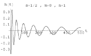 |
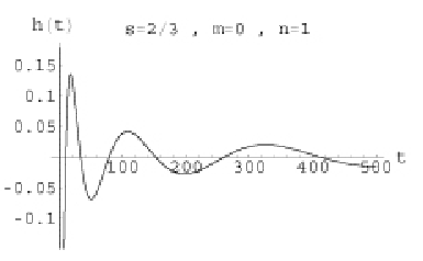 |
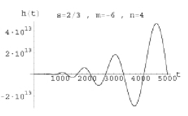 |
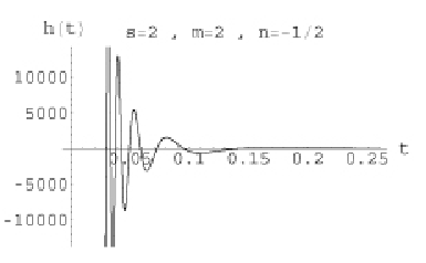 |
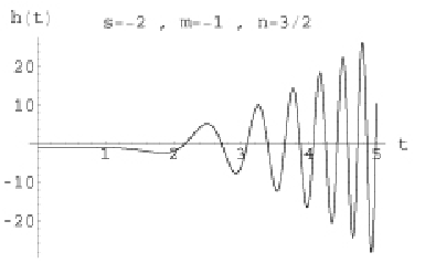 |
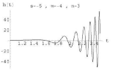 |
When the scale becomes larger than the Hubble radius , the growing mode of evolution is constant, i.e. it is frozen. It can be shown that , as an upper limit to , since other effects can contribute to the background anisotropy. From this consideration, it is clear that the only relevant quantity is the initial amplitude in Eq. (130), which is conserved until the reenter. Such an amplitude depends on the fundamental mechanism generating perturbations. Inflation gives rise to processes capable of producing perturbations as zero-point energy fluctuations. Such a mechanism depends on the gravitational interaction and then could constitute a further constraint to select a suitable theory of gravity. Considering a single graviton in the form of a monochromatic wave, its zero-point amplitude is derived through the commutation relations:
| (132) |
calculated at a fixed time , where the amplitude is the field and is the conjugate momentum operator. Writing the Lagrangian for
| (133) |
in the conformal FRW metric , where the amplitude is conformally invariant, we obtain
| (134) |
Eq. (132) becomes
| (135) |
and the fields and can be expanded in terms of creation and annihilation operators
| (136) |
| (137) |
The commutation relations in conformal time are
| (138) |
From (130) and (131), we obtain , where and are calculated at the first horizon-crossing and, being , the remarkable relation
| (139) |
holds for a generic theory at a given . Clearly the amplitude of GWs produced during inflation depends on the theory of gravity which, if different from GR, gives extra degrees of freedom. On the other hand, the Sachs-Wolfe effect could constitute a test for gravity at early epochs. This probe could give further constraints on the GW-stochastic background, if ETGs are independently probed at other scales.
In summary, the amplitudes of tensor GWs are conformally invariant and their evolution depends on the cosmological background. Such a background is tuned by a conformal scalar field which is not present in the standard GR. Assuming that primordial vacuum fluctuations produce stochastic GWs, beside scalar perturbations, kinematical distortions and so on, the initial amplitude of these ones is a function of the -theory of gravity and then the stochastic background can be, in a certain sense “tuned” by the theory. Viceversa, data coming from the Sachs-Wolfe effect could contribute to select a suitable theory which can be consistently matched with other observations. However, further and accurate studies are needed in order to test the relation between Sachs-Wolfe effect and gravity. This goal could be achieved very soon through the forthcoming space (LISA) and ground-based (VIRGO, LIGO) interferometers.
VI Applications to galactic dynamics
The results obtained at cosmological scales motivates further applications of ETGs, in particular of theories. In general, one is wondering whether ETG models, working as dark energy models, can also play a role to explain the dark matter phenomenology at scales of galaxies and clusters of galaxies.
Several studies have been pursued in this direction mond but the main goal remains that to seek a unified model capable of explain dynamics at every scale without introducing ad hoc components.
VI.1 Dark matter as a curvature effect: the case of flat rotation curves of LSB galaxies
It is well known that, in the low energy limit, higher order gravity implies modified gravitational potentials schmidt; modpot. By considering the case of a pointlike mass and solving the vacuum field equations for a Schwarzschild - like metric noipla; mnras, one gets as exact solution from a theory , the modified gravitational potential :
| (140) |
where
| (141) |
which corrects the ordinary Newtonian potential by a power - law term. As we will see, it has to be and then . In particular, the best fit value will be and then . Standard units have been considered here. In particular, this correction sets in on scales larger than which value depends essentially on the mass of the system mnras. This quantity deserves some discussion. As shown in mnras, it is derived from the initial conditions of the models and it correlates with the core masses of the LSB galaxies which we have taken into account. In some sense, it is a sort of further gravitational radius, beside the standard Schwarzschild radius, which rules the central mass of the galaxies, and then it is different for different systems. It is interesting to note that, given a generic -order theory of gravity, it is possible to find out characteristic radii schmidt and it is intriguing to suspect that they could likely rule the structure and the stability of the astrophysical self-gravitating structures betty. But this is a working hypothesis which has to be firmly demonstrated.
The corrected potential (140) reduces to the standard for as it can be seen from the relation (141). The generalization of Eq.(140) to extended systems is straightforward. We simply divide the system in infinitesimal mass elements and sum up the potentials generated by each single element. In the continuum limit, we replace the sum with an integral over the mass density of the system taking care of eventual symmetries of the mass distribution mnras. Once the gravitational potential has been computed, one may evaluate the rotation curve and compare it with the data. For extended systems, one has typically to resort to numerical techniques, but the main effect may be illustrated by the rotation curve for the pointlike case :
| (142) |
Compared with the Newtonian result , the corrected rotation curve is modified by the addition of the second term in the r.h.s. of Eq.(142). For , the corrected rotation curve is higher than the Newtonian one. Since measurements of spiral galaxies rotation curves signal a circular velocity higher than those which are predicted on the basis of the observed luminous mass and the Newtonian potential, the above result suggests the possibility that such a modified gravitational potential may fill the gap between theory and observations without the need of additional dark matter. It is worth noticing that the corrected rotation curve is asymptotically vanishing as in the Newtonian case, while it is usually claimed that observed rotation curves are flat (i.e., asymptotically constant). Actually, observations do not probe up to infinity, but only show that the rotation curve is flat within the measurement uncertainties up to the last measured point. This fact by no way excludes the possibility that goes to zero at infinity.
| Id | Type | |||||
|---|---|---|---|---|---|---|
| UGC 1230 | 51 | 22.6 | 4.5 | 101 | 58.0 | Sm |
| UGC 1281 | 5.5 | 22.7 | 1.7 | 206 | 3.2 | Sdm |
| UGC 3137 | 18.4 | 23.2 | 2.0 | 297 | 43.6 | Sbc |
| UGC 3371 | 12.8 | 23.3 | 3.1 | 188 | 12.2 | Im |
| UGC 4173 | 16.8 | 24.3 | 4.5 | 178 | 21.2 | Im |
| UGC 4325 | 10.1 | 21.6 | 1.6 | 142 | 7.5 | SAm |
| NGC 2366 | 3.4 | 22.6 | 1.5 | 439 | 7.3 | IB(s)m |
| IC 2233 | 10.5 | 22.5 | 2.3 | 193 | 13.6 | SBd |
| NGC 3274 | 6.7 | 20.2 | 0.5 | 225 | 6.6 | SABd |
| NGC 4395 | 3.5 | 22.2 | 2.3 | 527 | 9.7 | SAm |
| NGC 4455 | 6.8 | 20.8 | 0.7 | 192 | 5.4 | SBd |
| NGC 5023 | 4.8 | 20.9 | 0.8 | 256 | 3.5 | Scd |
| DDO 185 | 5.1 | 23.2 | 1.2 | 136 | 1.6 | IBm |
| DDO 189 | 12.6 | 22.6 | 1.2 | 167 | 10.5 | Im |
| UGC 10310 | 15.6 | 22.0 | 1.9 | 130 | 12.6 | SBm |
In order to observationally check the above result, one can take into account samples of low surface brightness (LSB) galaxies with well measured HI + H rotation curves extending far beyond the visible edge of the system. LSB galaxies are known to be ideal candidates to test dark matter models since, because of their high gas content, the rotation curves can be well measured and corrected for possible systematic errors by comparing 21 - cm HI line emission with optical H and data. Moreover, they are supposed to be dark matter dominated so that fitting their rotation curves without this elusive component could be a strong evidence in favor of any successful alternative theory of gravity. The considered sample (Table II) contains 15 LSB galaxies with data on the rotation curve, the surface mass density of the gas component and - photometric band, disk photometry extracted from a larger sample selected by de Blok & Bosma dbb02. We assume the stars are distributed in a thin and circularly symmetric disk with surface density where the central surface luminosity and the disk scalelength are obtained from fitting to the stellar photometry. The gas surface density has been obtained by interpolating the data over the range probed by HI measurements and extrapolated outside this range.
| Id | ||||||
|---|---|---|---|---|---|---|
| UGC 1230 | 0.83 0.02 | -0.39 0.09 | 0.15 0.01 | 15.9 0.5 | 2.97/8 | 0.96 |
| UGC 1281 | 0.38 0.01 | -3.93 0.80 | 0.65 0.08 | 0.64 0.33 | 3.48/21 | 1.05 |
| UGC 3137 | 0.72 0.03 | -1.86 0.06 | 0.65 0.02 | 9.8 0.9 | 48.1/26 | 1.81 |
| UGC 3371 | 0.78 0.05 | -1.85 0.01 | 0.41 0.01 | 3.3 0.2 | 0.48/15 | 1.30 |
| UGC 4173 | 0.94 0.02 | -0.97 0.22 | 0.34 0.01 | 9.37 0.04 | 0.12/10 | 0.52 |
| UGC 4325 | 0.79 0.07 | -2.85 0.44 | 0.70 0.02 | 0.50 0.05 | 0.09/13 | 1.19 |
| NGC 2366 | 0.96 0.14 | -0.58 0.42 | 0.64 0.01 | 14.5 0.9 | 28.6/25 | 1.10 |
| IC 2233 | 0.42 0.01 | -3.50 0.05 | 0.64 0.01 | 1.29 0.06 | 6.1/22 | 2.10 |
| NGC 3274 | 0.71 0.03 | -2.30 0.19 | 0.55 0.03 | 2.3 0.3 | 17.6/20 | 2.7 |
| NGC 4395 | 0.13 0.02 | -3.68 0.31 | 0.14 0.01 | 7.6 0.3 | 37.7/52 | 1.40 |
| NGC 4455 | 0.87 0.05 | -2.32 0.07 | 0.83 0.01 | 0.42 0.04 | 3.3/17 | 1.12 |
| NGC 5023 | 0.81 0.02 | -2.54 0.05 | 0.53 0.02 | 0.91 0.06 | 8.9/30 | 2.50 |
| DDO 185 | 0.92 0.10 | -2.75 0.35 | 0.90 0.03 | 0.21 0.07 | 5.03/5 | 0.81 |
| DDO 189 | 0.54 0.08 | -2.40 0.61 | 0.63 0.04 | 4.2 0.7 | 0.44/8 | 1.08 |
| UGC 10310 | 0.72 0.04 | -1.87 0.04 | 0.59 0.02 | 1.39 0.04 | 2.90/13 | 1.02 |
When fitting to the theoretical rotation curve, there are three quantities to be determined, namely the stellar mass - to - light (M/L) ratio, and the theory parameters . It is worth stressing that, while fit results for different galaxies should give the same , is related to one of the integration constants of the field equations. As such, it is not a universal quantity and its value must be set on a galaxy - by - galaxy basis.


However, it is expected that galaxies having similar properties in terms of mass distribution have similar values of so that the scatter in must reflect somewhat the scatter in the terminal circular velocities. In order to match the model with the data, we perform a likelihood analysis for each galaxy, using, as fitting parameters , (with in kpc) and the gas mass fraction77 7 This is related to the ratio as with the gas (HI + He) mass, and the disk total mass and luminosity. . As it is evident considering the results from the different fits summarized in Table 3, the experimental data are successfully fitted by the model. In particular, the best fit range of , corresponding to gravity with (best fit value ), seems well overlaps the above mentioned range of fitting SNeIa Hubble diagram.
 |
 |
 |
 |
 |
 |
 |
 |
 |
 |
 |
 |
 |
 |
 |
However, these are only preliminary results which do not completely solve the problem of dark matter in galaxies by models coming from ETGs and do not fit the growth of structures. In any case, further evidences on the same line of thinking are coming from other samples of galaxies (where also high surface brightness galaxies are considered) salucci, or from galaxy clusters, where the dark matter range is completely different betty.
VI.2 Dark Matter Halos inspired by - gravity
At this point, it is worth wondering whether a link may be found between gravity and the standard approach based on dark matter haloes since both theories fit equally well the same data. The trait - de - union between these two different schemes can be found in the modified gravitational potential which induces a correction to the rotation curve in a similar manner as a dark matter halo does. As a matter of fact, it is possible to define an effective dark matter halo by imposing that its rotation curve equals the correction term to the Newtonian curve induced by gravity. Mathematically, one has to split the total rotation curve derived from gravity as where the second term is the correction. Considering, for simplicity a spherical halo where a thin exponential disk is embedded, one can write the total rotation curve as with the Newtonian disk rotation curve and the dark matter one, being its mass distribution. Equating the two expressions, we get :
| (143) |
with , , and88 8 Here and , with are the Bessel functions of first and second type. :
| (144) |
with only depending on the geometry of the system and “" indicating virial quantities. Eq.(143) defines the mass profile of an effective spherically symmetric dark matter halo whose ordinary rotation curve provides the part of the corrected disk rotation curve due to the addition of the curvature corrective term to the gravitational potential. It is evident that, from an observational viewpoint, there is no way to discriminate between this dark halo model and a power-law gravity model. Having assumed spherical symmetry for the mass distribution, it is straightforward to compute the mass density for the effective dark halo as . The most interesting features of the density profile are its asymptotic behaviors that may be quantified by the logarithmic slope which can be numerically computed as function of for fixed values of (or ). As expected, depends explicitly on , while enter indirectly through . The asymptotic values at the center and at infinity denoted as and result particularly interesting. It turns out that almost vanishes so that in the innermost regions the density is approximately constant. Indeed, is the value corresponding to models having an inner core such as the cored isothermal sphere BT87 and the Burkert model burk. Moreover, it is well known that galactic rotation curves are typically best fitted by cored dark halo models (see, e.g., GS04 and references therein). On the other hand, the outer asymptotic slope is between and , that are values typical of most dark halo models in literature. In particular, for one finds , which are quite similar to the value for the Burkert model . It is worth noticing that the Burkert model has been empirically proposed to provide a good fit to the LSB and dwarf galaxies rotation curves. The values of we find for our best fit effective dark halo therefore suggest a possible theoretical motivation for the Burkert - like models. Due to the construction, the properties of the effective dark matter halo are closely related to the disk one. As such, we do expect some correlation between the dark halo and the disk parameters. To this aim, exploiting the relation between the virial mass and the disk parameters, one can obtain a relation for the Newtonian virial velocity :
| (145) |
One can numerically check that Eq.(145) may be well approximated as which has the same formal structure as the baryonic Tully - Fisher (BTF) relation with the total (gas + stars) baryonic mass and the circular velocity on the flat part of the observed rotation curve. In order to test whether the BTF can be explained thanks to the effective dark matter halo we are proposing, we should look for a relation between and . This is not analytically possible since the estimate of depends on the peculiarities of the observed rotation curve such as how far it extends and the uncertainties on the outermost points. Therefore, for given values of the disk parameters, it is possible to simulate theoretical rotation curves for some values of and measure finally choosing the fiducial value for which gives a value of as similar as possible to the measured one. Inserting the relation thus found between and into Eq.(145) and averaging over different simulations, one finally gets :
| (146) |
while a direct fit to the observed data gives ssm :
| (147) |
The slope of the predicted and observed BTF are in good agreement leading further support to the gravity model. The zeropoint is markedly different with the predicted one being significantly larger than the observed one, but it is worth stressing, however, that both relations fit the data with similar scatter. A discrepancy in the zeropoint may be due to the approximate treatment of the effective halo which does not take into account the gas component. Neglecting this term, one should increase the effective halo mass and hence which affects the relation with leading to a higher than observed zeropoint. Indeed, the larger is , the more the point deviate from our predicted BTF thus confirming our hypothesis. Given this caveat, we may therefore conclude with confidence that gravity offers a theoretical foundation even for the empirically found BTF relation.
All these results converge toward the picture that data coming from observations at galactic, extragalactic and cosmological scales could be seriously framed in ETGs without considering huge amounts of dark energy and dark matter.
VII Discussion and Conclusions
Extended Theories of Gravity can be considered as the natural extension of General Relativity. Also if they are not the final theory of gravity at fundamental level (i.e. quantum gravity), they could be a useful approach to address several shortcomings of GR. In fact, also at Solar System scales, where GR has been strongly confirmed, some conundrums come out as the indications of an apparent, anomalous, long-range acceleration revealed from the data analysis of Pioneer 10/11, Galileo, and Ulysses spacecrafts. Such results are difficult to be framed in the standard theory of GR and in its low energy limit anderson.
Furthermore, at galactic scales, huge bulks of dark matter are needed to provide realistic models matching with observations. In this case, retaining GR and its low energy limit, implies the introduction of an actually unknown ingredient (a huge amount of missing matter).
We face a similar situation even at larger scales: clusters of galaxies are gravitationally stable and bound only if large amounts of dark matter are supposed in their potential wells.
Finally, an unknown form of dark energy is required to explain the observed accelerated expansion of cosmic fluid. Summarizing, almost of matter-energy content of the Universe is unknown while we can experimentally probe only gravity and ordinary (baryonic and radiation) matter.
Considering another point of view, anomalous acceleration (Solar System), dark matter (galaxies, galaxy clusters and clustered structures in general), dark energy (cosmology) could be nothing else but the indications that gravity is an interaction depending on the scale and the assumption of a linear Lagrangian density in the Ricci scalar , as the Hilbert-Einstein action, could be too simple for a comprehensive picture at any scale.
Due to these facts, several motivations suggest to generalize GR by considering gravitational actions where generic functions of curvature invariants and scalar fields are present. This viewpoint is physically motivated by several unification schemes and by field quantization on curved spacetime birrell. Furthermore, it is well known that revisions of GR can solve shortcomings at early cosmological epochs (giving rise to suitable inflationary behaviors starobinsky; la) and explain the today observed accelerated behavior curvature; odinoj. These results can be achieved in metric and Palatini approaches noi-review; francaviglia_1; palatiniCosmo; multamaki.
In addition, reversing the problem, one can reconstruct the form of the gravity Lagrangian by observational data of cosmological relevance through a "back scattering" procedure mimick.
All these facts suggest that the theory should be more general than the linear Hilbert-Einstein one implying that extended gravity could be a suitable approach to solve GR shortcomings without introducing mysterious ingredients as dark energy and dark matter which seem without explanation at fundamental level. However, changing gravitational side could be nothing else but a matter of taste since final probes for dark energy and dark matter could come out from the forthcoming experiments as LHC.
Furthermore, in recent papers, some authors have confronted this kind of theories even with the PPN prescriptions considering both metric and Palatini approaches. The results seem controversial since in some cases olmo it is argued that GR is always valid and there is no room for other theories while other studies ppn-noi; mpla; allemandi-ruggiero find that recent experiments as Cassini and Lunar Laser Ranging allow the possibility that ETGs could be taken into account. In particular, it is possible to define generalized PPN-parameters and several ETGs could result compatible with experiments in Solar System will; mpla; damour.
In principle, any analytic ETGs can be compared with the Hilbert-Einstein Lagrangian provided suitable values of the coefficients. This consideration suggests to take into account, as physical theories, functions of the Ricci scalar which slightly deviates from GR, i.e. with a small parameter which indicates how much the theory deviates from GR and then approximate as
| (148) |
Actually, the PPN - Eddington parameters and may represent the key parameters to discriminate among relativistic theories of gravity. In particular, these quantities should be significatively tested at Solar System scales by forthcoming experiments like LATOR nordtvedt while the today available releases are far, in our opinion, to be conclusive in this sense, as a rapid inspection of Table IV suggests. In other words, ETGs cannot be a priori excluded also at Solar System scales.
| Mercury Perihelion Shift | |
|---|---|
| Lunar Laser Ranging | |
| Very Long Baseline Interf. | |
| Cassini Spacecraft |
In this paper, we have outlined what one should intend for ETGs in the metric and in the Palatini approach. In particular, we have discussed the higher-order and the scalar-tensor theories of gravity showing the relations between them and their connection to GR via the conformal transformations.
In the so called Einstein frame, any ETG can be reduced to the Hilbert-Einstein action plus one or more than one scalar field(s). The physical meaning of conformal transformations can be particularly devised in the Palatini approach, as discussed in Sec.IV. After, we have discussed some cosmological and astrophysical applications of ETGs.
Although the results outlined are referred to the simplest class of ETGs, power law , they could represent an interesting paradigm. Assuming both metric and Palatini approach, it is possible to investigate the viability of cosmological models. The expansion rate may be analytically expressed as a function of the redshift , so that it is possible to contrast the model predictions against the observations. In particular, the SNeIa Hubble diagram, the gas mass fraction in relaxed galaxy clusters, the lookback time to galaxy clusters, and radio galaxies can be used to constrain cosmological parameters by distance and time-based methods.
Also if such models are, up to now, not completely satisfactory to match all the observations, they allow to recover accelerated behavior of Hubble fluid without any unknown form of dark energy. However, the issue of structure formation has to be seriously faced in order to understand if such toy models could give rise to a self-consistent alternative theory to GR.
Furthermore, it is possible to "tune" the stochastic background of GWs and this occurrence could constitute a further cosmological test capable of confirming or ruling out ETGs once data from interferometers, like VIRGO, LIGO and LISA, will be available.
In addition, the modification of the gravitational potential arising as a natural effect in the framework of ETGs can represent a fundamental tool to interpret the rotation curves of spiral galaxies. Besides, if one considers the model parameters settled by the fit over the observational data on rotation curves, it is possible to construct a phenomenological analogous of dark matter halo whose shape is similar to the one of the so called Burkert model. Since Burkert’s model has been empirically introduced to give account for the dark matter distribution in the case of LSB and dwarf galaxies, this result could represent an interesting achievement since it provides a theoretical foundation to such a model.
By investigating the relation between dark halo and the galaxy disk parameters, a relation between and , reproducing the baryonic Tully - Fisher, can be deduced. In fact, exploiting the relation between the virial mass and the disk parameters, one obtains a relation for the virial velocity which can be satisfactory approximated as . Even such a result seems intriguing since it provides a theoretical interpretation for a phenomenological relation.
As a matter of fact, although not definitive, these phenomenological issues can represent a viable approach for future, more exhaustive investigations of ETGs. In particular, they support the quest for a unified view of the dark side of the Universe. In summary, these results seem to motivate a careful search for a fundamental theory of gravity capable of explaining the full cosmic dynamics by the only "ingredients" which we can directly and firmly experience, namely the background gravity, the baryonic matter, the radiation and also the neutrinos vitiello.
Acknowledgments
The authors wish to thank G. Allemandi, A. Borowiec, V.F. Cardone, S. Carloni, S. Nojiri, S.D. Odintsov, A. Stabile and A. Troisi for discussions, suggestions and results presented in this paper.
References
- (1) S. Weinberg, Gravitation and Cosmology, Wiley, 1972 New York N.Y.
- (2) A. Guth, Phys. Rev. D 23, 347 (1981).
- (3) I.L. Buchbinder, S.D. Odintsov, and I.L. Shapiro, Effective Action in Quantum Gravity, IOP Publishing (1992) Bristol.
- (4) H. Bondi, Cosmology, Cambridge Univ. Press, Cambridge (1952).
- (5) C. Brans and R.H. Dicke, Phys. Rev. 124, 925 (1961).
- (6) S. Capozziello, R. de Ritis, C. Rubano, and P. Scudellaro, La Rivista del Nuovo Cimento 4 (1996) 1.
- (7) D.W. Sciama, Mon. Not. R. Ast. Soc. 113, 34 (1953).
- (8) N.D. Birrell and P.C.W. Davies, Quantum Fields in Curved Space, Cambridge Univ. Press, Cambridge (1982).
- (9) G. Vilkovisky, Class. Quantum Grav. 9, 895 (1992).
- (10) M. Gasperini and G. Veneziano, Phys. Lett. 277B (1992) 256.
- (11) G. Magnano, M. Ferraris, and M. Francaviglia, Gen. Relativ. Grav. 19, 465 (1987).
- (12) J. Barrow and A.C. Ottewill, J. Phys. A: Math. Gen. 16, 2757 (1983).
- (13) A.A. Starobinsky, Phys. Lett. 91B (1980) 99.
- (14) J.P. Duruisseau and R. Kerner, Gen. Rel. Grav. 15, 797-807 (1983).
- (15) D. La and P.J. Steinhardt, Phys. Rev. Lett. 62 (1989) 376.
- (16) P. Teyssandier and Ph. Tourrenc, J. Math. Phys. 24, 2793 (1983).
- (17) K. Maeda, Phys. Rev. D 39, 3159 (1989).
- (18) D. Wands, Class. Quantum Grav. 11, 269 (1994).
- (19) S. Capozziello, R. de Ritis, A.A. Marino. Gen. Relativ. Grav. 30, 1247, (1998).
- (20) S. Gottlöber, H.-J. Schmidt, and A.A. Starobinsky, Class. Quantum Grav. 7, 893 (1990).
- (21) T.V. Ruzmaikina and A.A. Ruzmaikin, JETP, 30, 372 (1970).
- (22) L. Amendola, A. Battaglia-Mayer, S. Capozziello, S. Gottlöber, V. Müller, F. Occhionero and H.-J. Schmidt, Class. Quantum Grav. 10, L43 (1993).
- (23) A. Battaglia-Mayer and H.-J. Schmidt, Class. Quantum Grav. 10, 2441 (1993).
- (24) H.-J. Schmidt, Class. Quantum Grav. 7, 1023 (1990).
- (25) S. Capozziello, S. Nojiri, and S.D. Odintsov, Phys. Lett. B 634, 93 (2006).
- (26) L. Amendola, S. Capozziello, M. Litterio, F. Occhionero, Phys. Rev. D 45, 417 (1992).
- (27) S. Perlmutter et al., ApJ, 517, 565, 1999; R.A. Knop et al., ApJ, 598, 102, 2003.
- (28) A.G. Riess et al., AJ, 116, 1009, 1998; J.L. Tonry et al., ApJ, 594, 1, 2003.
- (29) P. de Bernardis et al., Nature, 404, 955, 2000
- (30) R. Stompor et al., ApJ, 561, L7, 2001
- (31) D.N. Spergel et al. ApJS, 148, 175, 2003.
- (32) G. Hinshaw et al. Ap. J. ApJS, 148, 135 (2003).
- (33) D.N. Spergel et al. astro-ph/0603449 (2006).
- (34) A.G. Riess et al., ApJ, 607, 665, 2004
- (35) V., Sahni, A. Starobinski, Int. J. Mod. Phys. D, 9, 373 (2000).
- (36) T. Padmanabhan, Phys. Rept., 380, 235 (2003).
- (37) E.J. Copeland, M. Sami, S. Tsujikawa, Int. Journ. Mod. Phys. D 15, 1753 (2006).
- (38) A. Kamenshchik, U. Moschella, V. Pasquier, Phys. Lett. B, 511, 265, 2001.
- (39) T. Padmanabhan, Phys. Rev. D, 66, 021301, 2002
- (40) B.A. Bassett, M. Kunz, D. Parkinson, C. Ungarelli, Phys. Rev. D, 68, 043504, 2003
- (41) V.F. Cardone, A. Troisi, S. Capozziello, Phys. Rev. D, 69, 083517, 2004; S. Capozziello, V.F. Cardone, E. Elizalde, S. Nojiri, S.D. Odintsov, Phys.Rev.D 73, 043512, 2006
- (42) A. Lue, R. Scoccimarro, G. Starkman, Phys. Rev. D, 69, 044005, 2004
- (43) K. Freese, M. Lewis, Phys. Lett. B, 540, 1, 2002
- (44) G.R. Dvali, G. Gabadadze, M. Porrati, Phys. Lett. B, 485, 208, 2000
- (45) S. Capozziello, Int. J. Mod. Phys. D, 11, 483, 2002; S. Nojiri and S.D. Odintsov, Phys. Rev. D, 68, 123512, 2003; Carroll, S.M., Duvvuri, V., Trodden, M., Turner, M.S., Phys. Rev. D, 70, 043528, 2004; G. Allemandi, A. Borowiec, M. Francaviglia, Phys. Rev. D, 70, 103503, 2004.
- (46) S.Nojiri and S.D. Odintsov, Int. J. Meth. Mod. Phys. 4, 115 (2007).
- (47) S. Capozziello, V.F. Cardone, E. Piedipalumbo, M. Sereno, A. Troisi, Int. J. Mod. Phys. D, 12, 381, 2003
- (48) S. Capozziello, V.F. Cardone, S. Carloni, A. Troisi, Int. J. Mod. Phys. D 12, 1969 (2003).
- (49) A.A. Starobinsky, astro-ph/0706.2041 (2007).
- (50) B. Li and J.D. Barrow, Phys. Rev. D75, 084010 (2007).
- (51) S.Nojiri and S.D. Odintsov, hep-th/06012113 (2006).
- (52) B. Li, J.D. Barrow and D.F. Mota, submitted to Phys. Rev. D, gr-qc/0705.3795.
- (53) G. Chen, B. Rathra, ApJ, 582, 586, 2003; S. Podariu, R.A. Daly, M.P. Mory, B. Rathra, ApJ, 584, 577, 2003.
- (54) C.M. Will, Theory and Experiments in Gravitational Physics (1993) Cambridge Univ. Press, Cambridge.
- (55) F.W. Hehl et al., Rev. Mod. Phys. 48, 393 (1976).
- (56) S. Capozziello, G. Lambiase and C. Stornaiolo, Ann. Phys. (Leipzig), 10, 713 (2001).
- (57) K. Stelle, Gen. Relativ. Grav. 9 (1978) 353.
- (58) R.H. Sanders, Ann. Rev. Astr. Ap. 2 (1990) 1.
- (59) P.D. Mannheim and D. Kazanas, Ap. J. 342 (1989) 635.
- (60) J.D. Anderson, et al., Phys. Rev. D 65 (2002) 082004.
- (61) O. Bertolami, Ch.G. Böhmer, F.S.N. Lobo, (2007) gr - qc/0704.1733
- (62) I. Quant and H.-J. Schmidt, Astron. Nachr. 312 (1991) 97.
- (63) P. Schneider, J. Ehlers, and E.E. Falco, Gravitational Lenses Springer–Verlag (1992) Berlin.
- (64) L.M. Krauss and M. White, Ap. J. 397 (1992) 357.
- (65) Ferraris M, Francaviglia M and Magnano G 1988 Class. Quantum Grav. 5 L95.
- (66) Sokolowski L M 1989 Class. Quantum Grav. 6 2045
- (67) G. Magnano and L.M. SokoLowski, Phys. Rev. D50, 5039 (1994).
- (68) Dicke R H 1962 Phys. Rev. 125 2163
- (69) Damour T and Esposito-Farèse G 1992 Class. Quantum Grav. 9 2093.
- (70) S. Capozziello, R. de Ritis, A.A. Marino, Class. Quantum Grav. 14, 3243 (1997).
- (71) V. Faraoni, Cosmology in Scalar-Tensor Gravity, Kluwer Academic, Dordrecht (2004).
- (72) A. Einstein, Sitzung-ber. Preuss. Akad. Wiss., 414 (1925).
- (73) H.A. Buchdahl, J. Phys. A 12 (8) (1979), 1229.
- (74) M. Ferraris, M. Francaviglia, C. Reina, Gen. Relativ. Grav. 14, 243 (1982).
- (75) M. Ferraris, M. Francaviglia and I. Volovich, Class. Quantum Grav. 11, 1505 (1994).
- (76) D.N. Vollick, Phys. Rev. D68, 063510 (2003).
- (77) B.Li and M.C. Chu, Phys. Rev. D74, 104010 (2006).
- (78) B.Li, K,C. Chan, and M.C. Chu, Phys. Rev. D,in press, astro-ph/0610794 (2006).
- (79) G. Allemandi, M. Capone, S. Capozziello, M. Francaviglia, Gen. Relativ. Grav. 38 (2006) 33.
- (80) X. Meng and P. Wang, GRG 36 (8), 1947 (2004); GRG 36 (12), 2673 (2004).
- (81) A. Einstein, Ann. der Physik 49 (1916) 769.
- (82) L.P. Eisenhart, Riemannian Geometry Princeton Univ. Press, Princeton (1955).
- (83) E. Schrödinger, Space-Time Structure, Cambridge Univ. Press, Cambridge (1960).
- (84) T. Levi-Civita, The Absolute Differential Calculus, Blackie and Son, London (1929).
- (85) O. Klein, New Theories in Physics, 77, Intern.Inst. of Intellectual Co-operation, League of Nations (1938).
- (86) E. Cartan, Ann. Ec. Norm. 42 (1925) 17.
- (87) A. Palatini, Rend. Circ. Mat. Palermo 43 (1919), 203.
- (88) V.I. Arnold, Mathematical Methods of Classical Mechanics, Springer-Verlag, Berlin (1978).
- (89) T. Appelquist, A. Chodos, P.G.O. Freund, Modern Kaluza-Klein Theories, Addison-Wesley, Reading (1987).
- (90) M. Kaku, Quantum Field Theory, Oxford Univ. Press, Oxford (1993).
- (91) M.B. Green, J.H. Schwarz, E. Witten, Superstring Theory, Cambridge Univ. Press, Cambridge (1987).
- (92) Damour T., Esposito-Farese G., Class. Quant. Grav. 9, 2093 (1992).
- (93) M. Ferraris, M.Francaviglia, in: Mechanics, Analysis and Geometry: 200 Years after Lagrange; Editor: M. Francaviglia, Elsevier Science Publishers B:V:, ().
- (94) S. Capozziello, R.de Ritis, C. Rubano, P. Scudellaro, Int. Journ. Mod. Phys. D 5, 85 (1996).
- (95) S. Capozziello and R. de Ritis, Class. Quantum Grav. 11 (1994) 107.
- (96) V. Sahni and A. Starobinsky, Int. J. Mod. Phys. D9, 373 (2000).
- (97) S. Capozziello, V.F. Cardone, M. Funaro, S. Andreon, Phys. Rev. D 70, (2004) 123501.
- (98) S. Capozziello, V. F. Cardone, A. Troisi, Phys. Rev. D 71, 043503 (2005).
- (99) S. Capozziello, V. F. Cardone, E. Piedipalumbo, C. Rubano, Class. Quant. Grav. 23, 1205 (2006).
- (100) S. Hannestad, E. Mortsell, Phys. Rev. D 66, 0635088 (2002); A. Melchiorri, L. Mersini, C. J. Odman, M. Trodden, Phys. Rev. D 68, 043509 (2003); S. Hannestad, E. Mortsell, JCAP 0409, 001 (2004).
- (101) Y. Song, W. Hu, I. Sawicki, Phys. Rev. D 75, 044004 (2007).
- (102) S. Tsujikawa, astro-ph/0705.1032 (2007).
- (103) T. Koivisto, Phys. Rev. D 73, 083517 (2006).
- (104) S. Boughn and R. Crittenden, Nature (London) 427, 45 (2004); P. Fasalba and E. Gaztanaga, MNRAS 350, L37 (2004); M.R. Nolta et al. Ap. J. 608, 10 (2004); P. Zhang, M. Liguori, R. Bean, and S. Dodelson, astro-ph/0704.1932 (2007).
- (105) S. Capozziello Int. Jou. of Geom. Methods in Mod. Phys. 4 (2007) 53.
- (106) M. Tegmark et al., Phys. Rev. D, 69, 103501, 2004
- (107) R. Rebolo et al., astro - ph/0402466, 2004
- (108) R.A. Daly, S.G. Djorgovski, astro - ph/0403664,2004
- (109) W.L. Freedman et al., ApJ, 553, 47, 2001.
- (110) V.F. Cardone, S. Capozziello, V. Re, E. Piedipalumbo, A&A, 382, 792, 2002
- (111) R. Saunders et al., MNRAS, 341, 937, 2003; R.W. Schmidt, S.W. Allen, A.C. Fabian, MNRAS, 352, 1413, 2004
- (112) Y. Wang, P. Mukherjee, ApJ, 606, 654, 2004
- (113) Y. Wang, M. Tegmark, Phys. Rev. Lett., 92, 241302, 2004
- (114) W. Hu, N. Sugiyama, ApJ, 471, 542, 1996
- (115) D. Kirkman, D. Tyler, N. Suzuki, J.M. O’Meara, D. Lubin, ApJS, 149, 1, 2003
- (116) D. Eisenstein et al., ApJ. 633, 560, 2005.
- (117) M.A. Strauss et al., AJ, 124, 1810., 2005.
- (118) SNAP web page : http://snap.lbl.gov
- (119) V. Faraoni, Class. Quantum Grav. 22, 32352 (2005).
- (120) C. Rubano and P. Scudellaro, Gen. Relativ. Grav. 37, 521 (2005).
- (121) S. Sasaki, PASJ, 48, L119, 1996; U. Pen, New Ast., 2, 309, 1997
- (122) S.W. Allen, R.W. Schmidt, A.C. Fabian, MNRAS, 334, L11, 2002; S.W. Allen, R.W. Schmidt, S. Bridle, MNRAS, 346, 593, 2003
- (123) S.W. Allen, R.W. Schmidt, H. Ebeling, A.C. Fabian, L. van Speybrock, astro - ph/0405340, 2004
- (124) V. Eke, J.F. Navarro, C.S. Frenk, ApJ, 503, 569, 1998
- (125) W.L. Freedman et al., ApJ, 553, 47, 2001.
- (126) M. Tegmark et al., astro - ph/0310723.
- (127) N. Dalal, K. Abazajian, E. Jenkins, A.V. Manohar, Phys. Rev. Lett., 87, 141302, 2001.
- (128) J.A.S. Lima, J.S. Alcaniz, MNRAS, 317, 893, 2000
- (129) G. Worthey, Ph.D. Thesis California Univ., Santa Cruz, 1992
- (130) R.G. Bower, T. Kodama, A. Terlevich, MNRAS, 299, 1193, 1998
- (131) S. Andreon, C. Lobo, A. Iovino, MNRAS, 349, 889, 2004
- (132) T. Kodama, N. Arimoto, 1997, A&A, 320, 41
- (133) S. Andreon, A&A, 409, 37, 2003.
- (134)
J. B. Wyithe, A. Loeb, and D.G. Barnes
ApJ, 634, 715, (2005).
M. McQuinn et al. ApJ 653, 815 (2006).
K Sigurdson, A Cooray, Phys. Rev. Lett. 95, 211303 (2005). - (135) J.P. Blakeslee et al., ApJ, 596, L143, 2003.
- (136) R. Cayrel et al., Nature, 409, 691, 2001.
- (137) Daly R.A., Djorgovsky S.G., 2004, Astrophys. J., 612, 652
- (138) Spergel D.N., et a., 2006, arXiv: astro-ph/0603449
- (139) Capozziello S., Nojiri S., Odintsov S.D., Troisi A., 2006, Phys. Lett. B (2006) 135.
- (140) L. Amendola, D. Polarski, and S. Tsujikawa, Phys. Rev. Lett. 98, 131302 (2007).
- (141) L. Amendola, R. Gannouji, D. Polarski, and S. Tsujikawa, Phys. Rev. D75, 083504 (2007).
- (142) S. Carloni, P. Dunsby, S. Capozziello, A. Troisi, Class. Quant. Grav. 22, 4839 (2005).
- (143) S. Carloni, A. Troisi, P.K.S. Dunsby, gr-qc/0706.0452 (2007).
- (144) Hwang J.C., Noh H., 1996, Phys. Rev. D, 54, 1460; Hwang J.C., Noh H., 2001, Phys. Lett. B, 506, 13.
- (145) Zhang P., 2006, Phys. Rev. D, 73, 123504
- (146) Mukhanov V.F., Feldman H.A., Brandenberger R.H., 1992, Phys. Rept. 215, 203
- (147) Lahav O., et al., 2002, MNRAS, 333, 961.
- (148) S. Capozziello, V.F. Cardone, M. Francaviglia, Gen. Relativ. Grav. 38 (2006) 711.
- (149) S. Capozziello, Ch. Corda, Int. Jou. Mod. Phys. D 15, (2006) 1119; S. Capozziello, Ch. Corda, M. De Laurentis Mod. Phys. Lett. A 22, (2007) 1097; S. Capozziello, M. De Laurentis, M. Francaviglia submitted to Int. Jou. Mod. Phys. D (2007).
- (150) Milgrom M. 1983, Astroph. Journ., 270, 365; Bekenstein J. 2004, Phys. Rev. D, 70, 083509.
- (151) Stelle K. 1978, Gen. Rel. Grav., 9, 353
- (152) Capozziello S., Cardone V.F., Carloni S., Troisi A. 2004, Phys. Lett. A, 326, 292
- (153) S. Capozziello, V.F. Cardone, A. Troisi, JCAP 0608 (2006) 1423.
- (154) S. Capozziello, V.F. Cardone, A. Troisi, MNRAS 375 (2007) 1423.
- (155) de Blok W.J.G., Bosma A. 2002, Astron. Astroph., 385, 816
- (156) C. Frigerio Martins, P. Salucci, astro - ph/07032443.
- (157) S. Capozziello, E. De Filippis, V. Salzano, in preparation.
- (158) Binney J., Tremaine S. 1987, Galactic dynamics, Princeton University Books
- (159) Burkert A. 1995, Astroph. Journ., 447, L25; Burkert A., Silk J. 1997, Astroph. Journ., 488, L55; Borriello A., Salucci P. 2001, Mont. Not. Roy. Astron. Soc., 323, 285
- (160) Gentile G., Salucci P. 2004, Mon. Not. Roy. Astron. Soc., 351, 953
- (161) McGaugh S.S. 2005, Astroph. Journ., 632, 859.
- (162) Capozziello, S., Carloni, S. and Troisi, A., Rec. Res. Devel. Astronomy. & Astrophys. 1, 625 (2003), astro-ph/0303041.
- (163) Allemandi G., Borowiec A., Francaviglia M., Phys. Rev. D 70, 043524 (2004).
- (164) Vollick D. N., Phys. Rev. D 68, 063510 (2003); Meng X. H., Wang P., Class. Quant. Grav. 20, 4949 (2003); Flanagan E. E., Phys. Rev. Lett. 92, 071101 (2004); Flanagan E. E., Class. Quant. Grav. 21, 417 (2004); Meng X. H., Wang P., Class. Quant. Grav. 21, 951 (2004); G. M. Kremer and D. S. M. Alves, Phys. Rev. D 70, 023503 (2004).
- (165) T. Multamaki and I. Vilja, Phys. Rev. D, 73, 024018, 2006.
- (166) Olmo G.J., Phys. Rev. Lett. 95, 261102 (2005); Olmo G.J., Phys. Rev. D 72, 083505 (2005).
- (167) Capozziello S., Troisi A., Phys. Rev. D 72 (2005).
- (168) S. Capozziello, A. Stabile, A. Troisi Mod. Phys. Lett.A 21 (2006) 2291.
- (169) Allemandi G., Francaviglia M., Ruggiero M., Tartaglia A., Gen. Rel. Grav. 37, 1891 (2005).
- (170) Turyshev S.G., Shao M., K.L. Nordtvedt K.L., pre-print: gr-qc/0601035.
- (171) Shapiro I.I., in General Relativity and Gravitation 12, Ashby N., et al., Eds. Cambridge University Press (1993).
- (172) Shapiro S.S., et al., Phys. Rev. Lett. D 92, 121101 (2004).
- (173) Williams J.G., et al., Phys. Rev. D 53, 6730 (1996).
- (174) Bertotti B., Iess L., Tortora P., Nature 425, 374 (2003).
- (175) A. Capolupo, S. Capozziello, G. Vitiello. Phys. Lett. A 363 (2007) 53.