跳到论文正文
W Papers独立论文阅读器 arXiv:0706.0973 论文正文 计算阅读时间 · 0%
引用这篇论文根据当前论文元数据生成,正式投稿前建议核对。


License: arXiv.org perpetual non-exclusive license
arXiv:0706.0973v3 [math.DG] 04 May 2009

Spacelike mean curvature one surfaces
in de Sitter 33-space

S. Fujimori Shoichi FujimoriDepartment of Mathematics, Fukuoka University of Education, Munakata, Fukuoka 811-4192, Japan Email address: fujimori@fukuoka-edu.ac.jp , W. Rossman Wayne RossmanDepartment of Mathematics, Faculty of Science, Kobe University, Rokko, Kobe 657-8501, Japan Email address: wayne@math.kobe-u.ac.jp , M. Umehara Masaaki UmeharaDepartment of Mathematics, Graduate School of Science, Osaka University, Toyonaka, Osaka 560-0043, Japan Email address: umehara@math.sci.osaka-u.ac.jp , K. Yamada Kotaro YamadaFaculty of Mathematics, Kyushu University, Higashi-ku, Fukuoka 812-8581, Japan Email address: kotaro@math.kyushu-u.ac.jp and S.-D. Yang Seong-Deog YangDepartment of Mathematics, Korea University, Seoul 136-701, Korea Email address: sdyang@korea.ac.kr
Abstract.

The first author studied spacelike constant mean curvature one (CMC-11) surfaces in de Sitter 3-space S13S^{3}_{1} when the surfaces have no singularities except within some compact subset and are of finite total curvature on the complement of this compact subset. However, there are many CMC-11 surfaces whose singular sets are not compact. In fact, such examples have already appeared in the construction of trinoids given by Lee and the last author via hypergeometric functions.

In this paper, we improve the Osserman-type inequality given by the first author. Moreover, we shall develop a fundamental framework that allows the singular set to be non-compact, and then will use it to investigate the global behavior of CMC-11 surfaces.

2000 Mathematics Subject Classification
Primary 53A10; Secondary 53A35, 53C50.

Introduction

A holomorphic map F:M2→SL2⁡𝑪F:M^{2}\to\operatorname{SL}_{2}\boldsymbol{C} of a Riemann surface M2M^{2} into the complex Lie group SL2⁡𝑪\operatorname{SL}_{2}\boldsymbol{C} is called null if det(d​F/d​z)\det(dF/dz) vanishes identically, where zz is a local complex coordinate of M2M^{2}. We consider two projections, one into the hyperbolic 33-space

πH:SL2⁡𝑪⟶H3=SL2⁡𝑪/SU2\pi_{H}:\operatorname{SL}_{2}\boldsymbol{C}\longrightarrow H^{3}=\operatorname{SL}_{2}\boldsymbol{C}/\operatorname{SU}_{2}

and the other into the de Sitter 33-space

πS:SL2⁡𝑪⟶S13=SL2⁡𝑪/SU1,1,\pi_{S}:\operatorname{SL}_{2}\boldsymbol{C}\longrightarrow S^{3}_{1}=\operatorname{SL}_{2}\boldsymbol{C}/\operatorname{SU}_{1,1},

where the definition of SU1,1\operatorname{SU}_{1,1} is in Appendix B. It is well-known that the projection of a holomorphic null immersion into H3H^{3} by πH\pi_{H} gives a conformal CMC-11 (constant mean curvature one) immersion (see [Br], [UY1], [CHR]). Moreover, conformal CMC-11 immersions are always given locally in such a manner.

On the other hand, spacelike CMC-11 surfaces given by the projection of holomorphic null immersions into S13S^{3}_{1} by πS\pi_{S} can have singularities, and are called CMC-11 faces. We work with this class of surfaces that is larger than the class of CMC-11 immersions. In fact, the class of CMC-11 immersions is too small, since there is only one, up to congruency, complete spacelike CMC-11 immersion [Ak, R], which we call an S13S^{3}_{1}-horosphere. (We also give a simple proof of this here. See the last remark of Section 1.)

The relationship between CMC-11 surfaces in H3H^{3} and CMC-11 faces in S13S^{3}_{1} is analogous to that between minimal surfaces in Euclidean 3-space 𝑹3\boldsymbol{R}^{3} and spacelike maximal surfaces with singularities in Lorentz-Minkowski 3-space 𝑹13\boldsymbol{R}_{1}^{3} (called maxfaces [UY5]). Note that maximal surfaces also admit a Weierstrass-type representation formula ([K]). As in the case of maxfaces (see [UY5]), the first author [F] investigated the global behavior of CMC-11 faces in S13S^{3}_{1}, in particular proving an Osserman-type inequality for complete CMC-11 faces of finite type whose ends are all elliptic, where a complete end of a CMC-11 face is called elliptic, parabolic, or hyperbolic if the monodromy matrix of the holomorphic lift F:M2→SL2⁡𝑪F:M^{2}\to\operatorname{SL}_{2}\boldsymbol{C} is elliptic, parabolic, or hyperbolic, respectively (see Section 1). One of our main results is the following, which implies that the ellipticity or parabolicity of ends follows from completeness:

Theorem I.

A complete end of a CMC-11 face in S13S_{1}^{3} is never hyperbolic, so must be either elliptic or parabolic. Moreover, the total curvature over a neighborhood of such an end is finite.

We remark that there exist incomplete elliptic and parabolic ends.

It is remarkable that just completeness of an end is sufficient to conclude that it has finite total curvature. This is certainly not the case for CMC-11 surfaces in H3H^{3} nor for minimal surfaces in 𝑹3\boldsymbol{R}^{3}, but is similar to the case of maximal surfaces in 𝑹13\boldsymbol{R}^{3}_{1} [UY5]. Although the asymptotic behavior of regular elliptic CMC-11 ends in S13S_{1}^{3} is investigated in [F], there do also exist complete parabolic ends, and to describe them, a much deeper analysis is needed, which we will conduct in this article.

As an application of Theorem I, we prove the following Osserman-type inequality, which improves the result of [F] by removing the assumptions of finite type and ellipticity of ends:

Theorem II.

Suppose a CMC-11 face f:M2→S13f\colon{}M^{2}\to S^{3}_{1} is complete. Then there exist a compact Riemann surface M¯2\overline{M}^{2} and a finite number of points p1,…,pn∈M¯2p_{1},\dots,p_{n}\in\overline{M}^{2} such that M2M^{2} is biholomorphic to M¯2∖{p1,…,pn}\overline{M}^{2}\setminus\{p_{1},\dots,p_{n}\}, and

(∗*) 2​deg⁡(G)≥−χ⁡(M¯2)+2​n,2\deg(G)\geq-\chi(\overline{M}^{2})+2n,

where GG is the hyperbolic Gauss map of ff and χ⁡(M¯2)\chi(\overline{M}^{2}) is the Euler characteristic of M¯2\overline{M}^{2}. Furthermore, equality holds if and only if each end is regular and properly embedded.

CMC-11 trinoids in S13S^{3}_{1} were constructed by Lee and the last author using hypergeometric functions [LY], and those trinoids with elliptic ends are complete in the sense of [F], and attain equality in ( ∗ ‣ II). However, those having other types of ends are not complete, as their singular sets are not compact. For this reason, our goal is not only to prove the above two theorems, but also to extend the framework for CMC-11 surfaces to include a larger class of surfaces, relaxing the immersedness and completeness conditions. If MM is of finite topology, i.e. if MM is diffeomorphic to a compact Riemann surface M¯2\overline{M}^{2} with finitely many punctures p1,…,pnp_{1},\dots,p_{n}, and if a CMC-11 face f:M2→S13f:M^{2}\to S^{3}_{1} is weakly complete, whose precise definition will be given in Section 1, we say that ff is a weakly complete CMC-11 face of finite topology. We shall develop the framework under this more general notion, which includes all the trinoids in [LY].

In Section 1, we recall definitions and basic results. In Section 2, we investigate the monodromy of the hyperbolic metrics on a punctured disk around an end. As an application, we prove Theorem I in Section 3. In Section 4, we give a geometric interpretation of the hyperbolic Gauss map. In Section 5, we investigate the asymptotic behavior of regular parabolic ends, and prove Theorem II. In Appendix A, we prove meromorphicity of the Hopf differential for complete CMC-11 faces. In Appendix B, we explain the conjugacy classes of SU1,1\operatorname{SU}_{1,1}.

Generic singularities of CMC-11 faces are classified in [FSUY]. A CMC-11 face is called embedded (in the wider sense) if it is embedded outside of some compact set of S13S^{3}_{1}. Examples of complete embedded CMC-11 faces are given in [FRUYY] as deformations of maxfaces in Lorentz-Minkowski 3-space 𝑹13\boldsymbol{R}_{1}^{3}.

1. Preliminaries

The representation formula

Let 𝑹14\boldsymbol{R}^{4}_{1} be the Lorentz-Minkowski space of dimension 44, with the Lorentz metric

⟨(x0,x1,x2,x3),(y0,y1,y2,y3)⟩=−x0​y0+x1​y1+x2​y2+x3​y3.\langle(x_{0},x_{1},x_{2},x_{3}),(y_{0},y_{1},y_{2},y_{3})\rangle=-x_{0}y_{0}+x_{1}y_{1}+x_{2}y_{2}+x_{3}y_{3}.

Then de Sitter 33-space is

S13={(x0,x1,x2,x3)∈𝑹14;−x02+x12+x22+x32=1},S^{3}_{1}=\{(x_{0},x_{1},x_{2},x_{3})\in\boldsymbol{R}^{4}_{1}\,;\,-x_{0}^{2}+x_{1}^{2}+x_{2}^{2}+x_{3}^{2}=1\},

with metric induced from 𝑹14\boldsymbol{R}^{4}_{1}, which is a simply-connected Lorentzian 33-manifold with constant sectional curvature 11. We identify 𝑹14\boldsymbol{R}^{4}_{1} with the set of 2×22\times 2 Hermitian matrices Herm(2)={X∗=X}\operatorname{Herm}(2)=\{X^{*}=X\} (X∗:=t⁡X¯X^{*}:=\mathord{\mathopen{{\vphantom{\overline{X}}}{}^{t}}\overline{X}}) by

(1.1) X=(x0,x1,x2,x3)↔X=∑k=03xk​ek=(x0+x3x1+i​x2x1−i​x2x0−x3),X=(x_{0},x_{1},x_{2},x_{3})\leftrightarrow X=\sum_{k=0}^{3}x_{k}e_{k}=\begin{pmatrix}x_{0}+x_{3}&x_{1}+ix_{2}\\ x_{1}-ix_{2}&x_{0}-x_{3}\end{pmatrix},

where

(1.2) e0=(1001),e1=(0110),e2=(0i−i0),e3=(100−1)e_{0}=\begin{pmatrix}1&0\\ 0&1\end{pmatrix},~e_{1}=\begin{pmatrix}0&1\\ 1&0\end{pmatrix},~e_{2}=\begin{pmatrix}\hphantom{-}0&i\\ -i&0\end{pmatrix},~e_{3}=\begin{pmatrix}1&\hphantom{-}0\\ 0&-1\end{pmatrix}

and i=−1i=\sqrt{-1}. Then S13S^{3}_{1} is

S13={X;X∗=X,detX=−1}={Fe3F∗;F∈SL2𝑪}S^{3}_{1}=\{X\,;\,X^{*}=X\,,\det X=-1\}=\{Fe_{3}F^{*}\,;\,F\in\operatorname{SL}_{2}\boldsymbol{C}\}

with the metric

⟨X,Y⟩=−12trace(Xe2(t⁡Y)e2),⟨X,X⟩=−detX.\left\langle{X},{Y}\right\rangle=-\frac{1}{2}\operatorname{trace}\left(Xe_{2}(\mathord{\mathopen{{\vphantom{Y}}{}^{t}}Y})e_{2}\right),\qquad\left\langle{X},{X}\right\rangle=-\det X.

The projection πS:SL2⁡𝑪→S13\pi_{S}\colon{}\operatorname{SL}_{2}\boldsymbol{C}\to S^{3}_{1} mentioned in the introduction is written explicitly as πS​(F)=F​e3​F∗\pi_{S}(F)=Fe_{3}F^{*}. Note that the hyperbolic 33-space H3H^{3} is given by H3={F​F∗;F∈SL2⁡𝑪}H^{3}=\{FF^{*}\,;\,F\in\operatorname{SL}_{2}\boldsymbol{C}\} and the projection is πH​(F)=F​F∗\pi_{H}(F)=FF^{*}.

An immersion into S13{S}^{3}_{1} is called spacelike if the induced metric on the immersed surface is positive definite. The complex Lie group SL2⁡𝑪\operatorname{SL}_{2}\boldsymbol{C} acts isometrically on Herm⁡(2)=𝑹14\operatorname{Herm}(2)=\boldsymbol{R}^{4}_{1}, as well as S13S^{3}_{1}, by

(1.3) Herm⁡(2)∋X⟼a​X​a∗a∈SL2⁡𝑪.\operatorname{Herm}(2)\ni X\longmapsto aXa^{*}\qquad a\in\operatorname{SL}_{2}\boldsymbol{C}.

In fact, PSL2𝑪=SL2𝑪/{±id}\operatorname{PSL}_{2}\boldsymbol{C}=\operatorname{SL}_{2}\boldsymbol{C}/\{\pm\operatorname{id}\} is isomorphic to the identity component SO3,1+\operatorname{SO}^{+}_{3,1} of the isometry group O3,1\operatorname{O}_{3,1} of S13S^{3}_{1}. Note that each element of SO3,1+\operatorname{SO}^{+}_{3,1} corresponds to an orientation preserving and orthochronous (i.e., time orientation preserving) isometry. The group of orientation preserving isometries of S13S^{3}_{1} is generated by PSL2⁡𝑪\operatorname{PSL}_{2}\boldsymbol{C} and the map

(1.4) S13∋X⟼−X∈S13.S^{3}_{1}\ni X\longmapsto-X\in S^{3}_{1}.

Aiyama-Akutagawa [AA] gave a Weierstrass-type representation formula in terms of holomorphic data for spacelike CMC-11 immersions in S13S^{3}_{1}. The first author [F] extended the notion of CMC-11 surfaces as follows, like as for the case of maximal surfaces in the Minkowski space [UY5].

Definition 1.1 ([F]).

Let M2M^{2} be a 22-manifold. A C∞C^{\infty}-map f:M2→S13f\colon{}M^{2}\to{S}^{3}_{1} is called a CMC-11 face if

  1. (1)

    there exists an open dense subset W⊂M2W\subset M^{2} such that f|Wf|_{W} is a spacelike CMC-11 immersion,

  2. (2)

    for any singular point (that is, a point where the induced metric degenerates) pp, there exists a C1C^{1}-differentiable function λ:U∩W→(0,∞)\lambda:U\cap W\to(0,\infty), defined on the intersection of neighborhood UU of pp with WW, such that λ​d​s2\lambda\,ds^{2} extends to a C1C^{1}-differentiable Riemannian metric on UU, where d​s2ds^{2} is the first fundamental form, i.e., the pull-back of the metric of S13S^{3}_{1} by ff, and

  3. (3)

    d​f​(p)≠0df(p)\neq 0 for any p∈M2p\in M^{2}.

Remark 1.2.

Though the original definition of CMC-11 faces in [F] assumed the orientability of the source manifold, our definition here does not. However, this difference is not of an essential nature. In fact, for any CMC-11 face f:M2→S13f:M^{2}\to S^{3}_{1}, M2M^{2} is automatically orientable. (See [KU].)

Remark 1.3.

A C∞C^{\infty}-map f:M2→S13f:M^{2}\to S^{3}_{1} is called a frontal if ff lifts to a C∞C^{\infty}-map Lf:M2→P⁡(T∗​S13)L_{f}\colon M^{2}\to P(T^{*}S^{3}_{1}) such that d​Lf​(T​M2)dL_{f}(TM^{2}) lies in the canonical contact plane-field on P⁡(T∗​S13)P(T^{*}S^{3}_{1}). Moreover, ff is called a wave front or a front if LfL_{f} is an immersion, that is, Lf​(M2)L_{f}(M^{2}) is a Legendrian submanifold. If a frontal LfL_{f} can lift up to a smooth map into T∗​S13T^{*}S^{3}_{1}, ff is called co-orientable, and otherwise it is called non-co-orientable. Wave fronts are a canonical class for investigating flat surfaces in the hyperbolic 3-space H3H^{3}. In fact, like for CMC-11 faces (see Theorem II in the introduction), an Osserman-type inequality holds for flat fronts in H3H^{3} (see [KUY2].) Although our CMC-11 faces belong to a special class of horospherical linear Weingarten surfaces (cf. [KU]), they may not be (wave) fronts in general, but are co-orientable frontals. In particular, there is a globally defined non-vanishing normal vector field ν\nu on the whole of M2M^{2} for a given CMC-11 face f:M2→S13f:M^{2}\to S^{3}_{1}. It should be remarked that the limiting tangent plane at each singular point contains a lightlike direction, that is, a CMC-11 face is not spacelike on the singular set.

An oriented 22-manifold M2M^{2} on which a CMC-11 face f:M2→S13f:M^{2}\to{S}^{3}_{1} is defined always has a complex structure (see [F]). Since CMC-11 faces are all orientable and co-orientable (cf. [KU]), from now on, we will treat M2M^{2} as a Riemann surface, and we can assume the existence of a globally defined non-vanishing normal vector field. The representation formula in [AA] can be extended for CMC-11 faces as follows:

Theorem 1.4 ([F, Theorem 1.9]).

Let M~2\widetilde{M}^{2} be a simply connected Riemann surface. Let gg be a meromorphic function and ω\omega a holomorphic 11-form on M~2\widetilde{M}^{2} such that

(1.5) d​s^2=(1+|g|2)2​|ω|2d\hat{s}^{2}=(1+|g|^{2})^{2}|\omega|^{2}

is a Riemannian metric on M~2\widetilde{M}^{2} and |g||g| is not identically 11. Take a holomorphic immersion F=(Fj​k):M~2→SL2⁡𝐂F=(F_{jk}):\widetilde{M}^{2}\to\operatorname{SL}_{2}\boldsymbol{C} satisfying

(1.6) F−1​d​F=(g−g21−g)​ω.F^{-1}dF=\begin{pmatrix}g&-g^{2}\\ 1&-g\hphantom{{}^{2}}\end{pmatrix}\omega.

Then f:M~2→S13f:\widetilde{M}^{2}\to{S}^{3}_{1} defined by

(1.7) f=πS∘F:=F​e3​F∗f=\pi_{S}\circ F:=Fe_{3}F^{*}

is a CMC-11 face which is conformal away from its singularities. The induced metric d​s2ds^{2} on M~2\widetilde{M}^{2}, the second fundamental form I​I, and the Hopf differential QQ of ff are given as follows:

(1.8) d​s2=(1−|g|2)2​|ω|2,I​I=Q+Q¯+d​s2,Q=ω​d​g.ds^{2}=(1-|g|^{2})^{2}|\omega|^{2},\quad\mbox{I\!I}=Q+\overline{Q}+ds^{2},\quad Q=\omega\,dg.

The singularities of the CMC-11 face occur at points where |g|=1|g|=1.

Conversely, for any CMC-11 face f:M~2→S13f:\widetilde{M}^{2}\to{S}^{3}_{1}, there exist a meromorphic function gg (with |g||g| not identically 11) and a holomorphic 11-form ω\omega on M~2\widetilde{M}^{2} so that d​s^2d\hat{s}^{2} is a Riemannian metric on M~2\widetilde{M}^{2} and (1.7) holds, where F:M~2→SL2⁡𝐂F:\widetilde{M}^{2}\to\operatorname{SL}_{2}\boldsymbol{C} is an immersion satisfying (1.6).

Remark 1.5.

By definition, CMC-11 faces have dense regular sets. However, the projection of null holomorphic immersions might not have dense regular sets, in general. Such an example has been given in [F, Remark 1.8]. Fortunately, we can explicitly classify such degenerate examples, as follows: Let M2M^{2} be a connected Riemann surface and F:M2→SL⁡(2,𝑪)F\colon{}M^{2}\to\operatorname{SL}(2,\boldsymbol{C}) be a null immersion. We assume that the set of singular points of the corresponding map

f=F​e3​F∗:M2⟶S13f=F{e_{3}}F^{*}\colon{}M^{2}\longrightarrow S^{3}_{1}

has an interior point. Then the secondary Gauss map gg is constant on M2M^{2} and |g|=1|g|=1. Without loss of generality, we may assume g=1g=1. Since FF is an immersion, (1+|g|2)2​|ω|2(1+|g|^{2})^{2}|\omega|^{2} is positive definite. Then ω≠0\omega\neq 0 everywhere. Hence for each p∈M2p\in M^{2}, one can take a complex coordinate zz such that ω=d​z\omega=dz. Then FF is a solution of

F−1​d​F=(1−11−1)​d​z.F^{-1}dF=\begin{pmatrix}1&-1\\ 1&-1\end{pmatrix}dz.

Without loss of generality, we may assume that F⁡(0)=(1/21/2−11)F(0)=\begin{pmatrix}{1}/{2}&{1}/{2}\\ -1&1\end{pmatrix}. Then we have

F=(z+1/2−z+1/2−11),F=\begin{pmatrix}z+{1}/{2}&-z+{1}/{2}\\ -1&1\end{pmatrix},

and the corresponding map ff is computed as

f=F​e3​F∗=(2​Re⁡z−1−10),f=Fe_{3}F^{*}=\begin{pmatrix}2\operatorname{Re}z&-1\\ -1&0\end{pmatrix},

whose image is a lightlike line in S13S^{3}_{1}. Thus, we have shown that the image of any degenerate CMC-11 surface is a part of a lightlike line.

Remark 1.6.

Theorem 1.4 is an analogue of the Bryant representation for CMC-11 surfaces in H3H^{3}, which explains why CMC-11 surfaces in both H3H^{3} and S13S^{3}_{1} are characterized by the projections πH∘F\pi_{H}\circ F and πS∘F\pi_{S}\circ F. The CMC-11 surfaces in H3H^{3} and S13S^{3}_{1} are both typical examples in the class of linear Weingarten surfaces. A Bryant-type representation formula for linear Weingarten surfaces was recently given by J. Gálvez, A. Martínez and F. Milán [GMM].

Remark 1.7.

Following the terminology of [UY1], gg is called a secondary Gauss map of ff. The pair (g,ω)(g,\omega) is called Weierstrass data of ff, and FF is called a holomorphic null lift of ff.

The holomorphic 22-differential QQ as in (1.8) is called the Hopf differential of ff. In analogy with the theory of CMC-11 surfaces in H3H^{3}, the meromorphic function

(1.9) G:=d​F11d​F21=d​F12d​F22G:=\frac{dF_{11}}{dF_{21}}=\frac{dF_{12}}{dF_{22}}

is called the hyperbolic Gauss map. A geometric meaning for the hyperbolic Gauss map is given in Section 4.

Remark 1.8.

Corresponding to Theorem 1.4, a Weierstrass-type representation formula is known for spacelike maximal surfaces in 𝑹13\boldsymbol{R}^{3}_{1} ([K]). In fact, the Weierstrass data (g,ω)(g,\omega) as in Theorem 1.4 defines null curves in 𝑪3\boldsymbol{C}^{3} by

F0​(z):=∫z0z(−2​g,1+g2,i⁡(1−g2))​ω.F_{0}(z):=\int_{z_{0}}^{z}\bigl(-2g,1+g^{2},i(1-g^{2})\bigr)\omega.

Any maxface (see [UY5] for the definition) is locally obtained as the real part of some F0F_{0}. Moreover, their first fundamental forms and Hopf differentials are given by (1.8). The meromorphic function gg can be identified with the Lorentzian Gauss map. In this case, we call the pair (g,ω)(g,\omega) the Weierstrass data of the maxface.

Remark 1.9.

Let G,gG,g be meromorphic functions on a Riemann surface. Set

(1.10) F=(G​d​ad​G−aG​d​bd​G−bd​ad​Gd​bd​G),a=d​Gd​g,b=−g​a.F=\begin{pmatrix}G\dfrac{da}{dG}-a&G\dfrac{db}{dG}-b\\[6.0pt] \dfrac{da}{dG}&\dfrac{db}{dG}\end{pmatrix},\qquad a=\sqrt{\frac{dG}{dg}},\quad b=-ga.

Then FF is a meromorphic null map with hyperbolic and secondary Gauss maps GG and gg. Formula (1.10) is called Small’s formula ([KUY1], [S]).

Remark 1.10.

The holomorphic null lift FF of a CMC-11 face ff is unique up to right-multiplication by matrices in SU1,1\operatorname{SU}_{1,1}, that is, for each A∈SU1,1A\in\operatorname{SU}_{1,1}, the projection of F​A−1FA^{-1} is also ff. Under the transformation F↦F​A−1F\mapsto FA^{-1}, the secondary Gauss map gg changes by a Möbius transformation:

(1.11) g⟼A⋆g:=A11​g+A12A21​g+A22,A=(A11A12A21A22).g\longmapsto A\star g:=\frac{A_{11}g+A_{12}}{A_{21}g+A_{22}},\qquad A=\begin{pmatrix}A_{11}&A_{12}\\ A_{21}&A_{22}\end{pmatrix}.

The conditions |g|=1|g|=1, |g|>1|g|>1, |g|<1|g|<1 are invariant under this transformation.

In particular, let f:M2→S13f\colon{}M^{2}\to S^{3}_{1} be a CMC-11 face of a (not necessarily simply connected) Riemann surface M2M^{2}. Then the holomorphic null lift FF is defined only on the universal cover M~2\widetilde{M}^{2} of M2M^{2}. Take a deck transformation τ∈π1​(M2)\tau\in\pi_{1}(M^{2}) in M~2\widetilde{M}^{2}. Since πS∘F=πS∘F∘τ\pi_{S}\circ F=\pi_{S}\circ F\circ\tau, there exists a ρ~​(τ)∈SU1,1\tilde{\rho}(\tau)\in\operatorname{SU}_{1,1} such that

(1.12) F∘τ=F​ρ~​(τ).F\circ\tau=F\tilde{\rho}(\tau).

The representation ρ~:π1​(M2)→SU1,1\tilde{\rho}\colon{}\pi_{1}(M^{2})\to\operatorname{SU}_{1,1} is called the monodromy representation, which induces a PSU1,1\operatorname{PSU}_{1,1}-representation ρ:π1​(M2)→PSU1,1=SU1,1/{±1}\rho\colon{}\pi_{1}(M^{2})\to\operatorname{PSU}_{1,1}=\operatorname{SU}_{1,1}/\{\pm 1\} satisfying

(1.13) g∘τ−1=ρ⁡(τ)⋆g.g\circ\tau^{-1}=\rho(\tau)\star g.
Remark 1.11.

The action F↦B​FF\mapsto BF, B∈SL2⁡𝑪B\in\operatorname{SL}_{2}\boldsymbol{C}, induces a rigid motion f↦B​f​B∗f\mapsto BfB^{*} in S13S^{3}_{1}, and the isometric motion f↦−ff\mapsto-f as in (1.4) corresponds to

(1.14) F⟼F♮=F​(0ii0)=i​F​e1.F\longmapsto F^{\natural}=F\begin{pmatrix}0&i\\ i&0\end{pmatrix}=iFe_{1}.

The secondary Gauss map of F♮F^{\natural} is 1/g1/g.

Remark 1.12.

Let Kd​s2K_{ds^{2}} be the Gaussian curvature of d​s2ds^{2} on the set of regular points of ff. Then

(1.15) d​σ2:=Kd​s2​d​s2=4​|d​g|2(1−|g|2)2d\sigma^{2}:=K_{ds^{2}}\,ds^{2}=\frac{4\,|dg|^{2}}{(1-|g|^{2})^{2}}

is a pseudometric of constant curvature −1-1, which degenerates at isolated umbilic points. We have

(1.16) d​σ2⋅d​s2=4​|Q|2.d\sigma^{2}\cdot ds^{2}=4|Q|^{2}.
Remark 1.13.

The metric

(1.17) d​s#2:=(1+|G|2)2​|Qd​G|2ds_{\#}^{2}:=\bigl(1+|G|^{2}\bigr)^{2}\left|\frac{Q}{dG}\right|^{2}

is induced from the canonical Hermitian metric of SL2⁡𝑪\operatorname{SL}_{2}\boldsymbol{C} via F−1:M~2→SL2⁡𝑪F^{-1}\colon{}\widetilde{M}^{2}\to\operatorname{SL}_{2}\boldsymbol{C}. When the CMC-11 face is defined on M2M^{2}, GG and QQ are as well, so d​s#2ds_{\#}^{2} is well-defined on M2M^{2}, and is called the lift metric. It is nothing but the dual metric of the CMC-11 surface πH∘F\pi_{H}\circ F in H3H^{3}, see [UY3].

Completeness

We now define two different notions of completeness for CMC-11 faces as follows:

Definition 1.14.

We say a CMC-11 face f:M2→S13f\colon M^{2}\to S^{3}_{1} is complete if there exists a symmetric 22-tensor field TT which vanishes outside a compact subset C⊂M2C\subset M^{2} such that the sum T+d​s2T+ds^{2} is a complete Riemannian metric on M2M^{2}.

See [F], with similar definitions in [KUY2] for flat fronts in H3H^{3} and in [UY5] for maxfaces.

Definition 1.15.

We say that ff is weakly complete if it is congruent to an S13S^{3}_{1}-horosphere or if the lift metric (1.17) is a complete Riemannian metric on M2M^{2}.

Here, the S13S^{3}_{1}-horosphere is the totally umbilic CMC-11 surface, which is also the only complete CMC-11 immersed surface (see Remark 1.21). It has the Weierstrass data g=c=constantg=c=\mbox{constant} (|c|≠1)(|c|\neq 1) and ω=d​z\omega=dz. The metric d​s#2ds^{2}_{\#} of an S13S^{3}_{1}-horosphere cannot be defined by (1.17) as GG is constant and QQ is identically 00, but can still be defined as the metric induced by F−1F^{-1}, and is a complete flat metric on 𝑪\boldsymbol{C}.

Definition 1.16.

We say that ff is of finite type if there exists a compact set CC of M2M^{2} such that the first fundamental form d​s2ds^{2} is positive definite and has finite total (absolute) curvature on M2∖CM^{2}\setminus C.

Let f:M2→S13f\colon{}M^{2}\to S^{3}_{1} be a CMC-11 face of finite topology, that is, M2M^{2} is diffeomorphic to a compact Riemann surface M¯2\overline{M}^{2} with a finite number of points {p1,…,pn}⊂M¯2\{p_{1},\dots,p_{n}\}\subset\overline{M}^{2} excluded. We can take a punctured neighborhood Δj∗\Delta_{j}^{*} of pjp_{j} which is biholomorphic to either the punctured unit disk Δ∗={z∈𝑪; 0<|z|<1}\Delta^{*}=\{z\in\boldsymbol{C}\,;\,0<|z|<1\} or an annular domain, and pjp_{j} is called a puncture-type end or an annular end, respectively.

Proposition 1.17.

Let f:M2→S13f:M^{2}\to S^{3}_{1} be a CMC-11 face. If ff is complete, then

  1. (1)

    the singular set of ff is compact,

  2. (2)

    ff is weakly complete,

  3. (3)

    M2M^{2} has finite topology and each end is of puncture-type.

Proof.

(1) is obvious. If ff is totally umbilic, it is congruent to an S13S^{3}_{1}-horosphere and the assertion is obvious. So we assume the Hopf differential QQ does not vanish identically. Since the Gaussian curvature of ff is nonnegative, completeness implies (3) by the appendix of [UY5]. So we shall now prove that completeness implies weak completeness: Fix an end pjp_{j} of ff. By an appropriate choice of a coordinate zz, the restriction of ff to a neighborhood of pjp_{j} is fj:Δ∗→S13f_{j}:\Delta^{*}\to S^{3}_{1}. We denote by d​s^2d\hat{s}^{2} the induced metric of the corresponding CMC-11 surface f^j=F​F∗:Δ~∗→H3\hat{f}_{j}=FF^{*}\colon{}\widetilde{\Delta}^{*}\to H^{3} into hyperbolic 33-space. Take a path γ:[0,1)→Δ∗\gamma\colon{}[0,1)\to\Delta^{*} such that γ⁡(t)→0\gamma(t)\to 0 as t→1t\to 1. Then by (1.5) and (1.8), d​s^2≥d​s2d\hat{s}^{2}\geq ds^{2} holds, and hence completeness of ff implies that each lift γ~:[0,1)→Δ~∗\tilde{\gamma}\colon{}[0,1)\to\widetilde{\Delta}^{*} of γ\gamma has infinite length with respect to d​s^2d\hat{s}^{2}. Here, d​s^2d\hat{s}^{2} and d​s#2=(1+|G|2)2​|Q/d​G|2ds^{2}_{\#}=(1+|G|^{2})^{2}|Q/dG|^{2} are the pull-backs of the Hermitian metric of SL2⁡𝑪\operatorname{SL}_{2}\boldsymbol{C} by FF and F−1F^{-1}, respectively. Yu [Y] showed that completeness of these two metrics are equivalent. Hence, γ~\tilde{\gamma} has infinite length with respect to the metric d​s#2ds^{2}_{\#}. Since d​s#2ds^{2}_{\#} is well-defined on Δ∗\Delta^{*}, γ\gamma also has infinite length with respect to d​s#2ds^{2}_{\#}, that is, the metric d​s#2ds^{2}_{\#} on Δ∗\Delta^{*} is complete at 00. Thus, fjf_{j} is a weakly complete end. ∎

For further properties of complete ends, see Theorems 3.10 and 3.11.

Remark 1.18.

Our definition of weak completeness of CMC-11 faces is somewhat more technical than that of maxfaces [UY5], but it is the correctly corresponding concept in S13S_{1}^{3}: for data (g,ω)(g,\omega), weak completeness of the associated maxface in 𝑹13\boldsymbol{R}_{1}^{3} is equivalent to that of the CMC-11 face in S13S^{3}_{1}.

Remark 1.19.

The CMC-11 trinoids in S13S^{3}_{1} constructed in [LY] are all weakly complete (sometimes complete as well) and all ends are gg-regular, see Section 3.

Remark 1.20.

The Hopf differential QQ of a complete CMC-11 face f:M2→S13f:M^{2}\to S^{3}_{1} is meromorphic on its compactification M¯2\overline{M}^{2}, even without assuming that all ends of ff are regular. See Appendix A. It should be remarked that for CMC-11 surfaces in hyperbolic 33-space, finiteness of total curvature is needed to show the meromorphicity of QQ (see [Br]).

Monodromy of ends of CMC-11 faces

For any real number tt, we set

(1.18) Λe​(t)\displaystyle\Lambda_{e}(t) :=(ei​t00e−i​t),\displaystyle:=\begin{pmatrix}e^{it}&0\\ 0&e^{-it}\end{pmatrix},
Λp​(t)\displaystyle\Lambda_{p}(t) :=(1+i​t−i​ti​t1−i​t),\displaystyle:=\begin{pmatrix}1+it&-it\\ it&1-it\end{pmatrix},
Λh​(t)\displaystyle\Lambda_{h}(t) :=(cosh⁡tsinh⁡tsinh⁡tcosh⁡t).\displaystyle:=\begin{pmatrix}\cosh t&\sinh t\\ \sinh t&\cosh t\end{pmatrix}.

A matrix in SU1,1\operatorname{SU}_{1,1} is called

  1. (1)

    elliptic if it is conjugate to Λe​(t)\Lambda_{e}(t) (t∈(−π,π]t\in(-\pi,\pi]) in SU1,1\operatorname{SU}_{1,1},

  2. (2)

    parabolic if it is conjugate to ±Λp​(t)\pm\Lambda_{p}(t) (t∈𝑹∖{0}t\in\boldsymbol{R}\setminus\{0\}) in SU1,1\operatorname{SU}_{1,1}, and

  3. (3)

    hyperbolic if it is conjugate to ±Λh​(t)\pm\Lambda_{h}(t) (t>0t>0) in SU1,1\operatorname{SU}_{1,1}.

Any matrix in SU1,1\operatorname{SU}_{1,1} is of one of these three types, see Appendix B. Note that the parabolic matrices Λp​(t1)\Lambda_{p}(t_{1}) and Λp​(t2)\Lambda_{p}(t_{2}) are conjugate in SU1,1\operatorname{SU}_{1,1} if and only if t1​t2>0t_{1}t_{2}>0. Though the set of conjugate classes of parabolic matrices is fully represented by {±Λp​(±1)}\{\pm\Lambda_{p}(\pm 1)\}, we may use various values of tt in this paper for the sake of simplicity.

Let f:M2→S13f\colon M^{2}\to S^{3}_{1} be a weakly complete CMC-11 face of finite topology, where M2M^{2} is diffeomorphic to a compact Riemann surface M¯2\overline{M}^{2} with finitely many punctures {p1,…,pn}\{p_{1},\dots,p_{n}\}. Any puncture pjp_{j}, or occasionally a small neighborhood UjU_{j} of pjp_{j}, is called an end of ff.

An end is called elliptic, parabolic or hyperbolic when the monodromy matrix ρ~​(τ)∈SU1,1\tilde{\rho}(\tau)\in\operatorname{SU}_{1,1} is elliptic, parabolic or hyperbolic, respectively, where ρ~\tilde{\rho} is as in Remark 1.10 and τ∈π1​(M2)\tau\in\pi_{1}(M^{2}) is the deck transformation corresponding to the counterclockwise loop about pjp_{j}.

The Schwarzian derivative

Let (U,z)(U,z) be a local complex coordinate of a Riemann surface M2M^{2}, and h⁡(z)h(z) a meromorphic function on UU. Then

Sz(h):=(h′′h′)′−12(h′′h′)2(=′dd​z)S_{z}(h):=\left(\frac{h^{\prime\prime}}{h^{\prime}}\right)^{\prime}-\frac{1}{2}\left(\frac{h^{\prime\prime}}{h^{\prime}}\right)^{2}\qquad\left({}^{\prime}=\frac{d}{dz}\right)

is the Schwarzian derivative of hh with respect to the coordinate zz.

If h⁡(z)=a+b​(z−p)m+o⁡((z−p)m)h(z)=a+b(z-p)^{m}+o\bigl((z-p)^{m}\bigr) at z=pz=p (b≠0)(b\neq 0), where o⁡((z−p)m)o\bigl((z-p)^{m}\bigr) denotes higher order terms, then the positive integer mm is called the (ramification) order of h⁡(z)h(z), and we have

(1.19) Sz​(h)=1(z−p)2​(1−m22+o⁡(1)).S_{z}(h)=\frac{1}{(z-p)^{2}}\left(\frac{1-m^{2}}{2}+o(1)\right).

We write S⁡(h)=Sz​(h)​d​z2S(h)=S_{z}(h)\,dz^{2}, which we also call the Schwarzian derivative. The Schwarzian derivative depends on the choice of local coordinates, but the difference does not, that is, S⁡(h1)−S⁡(h2)S(h_{1})-S(h_{2}) is a well-defined holomorphic 22-differential.

The Schwarzian derivative is invariant under Möbius transformations: S⁡(h)=S⁡(A⋆h)S(h)=S(A\star h) holds for A∈SL2⁡𝑪A\in\operatorname{SL}_{2}\boldsymbol{C}, where ⋆\star denotes the Möbius transformation as in (1.11). Conversely, if S⁡(h)=S⁡(g)S(h)=S(g), there exists an A∈SL2⁡𝑪A\in\operatorname{SL}_{2}\boldsymbol{C} such that g=A⋆hg=A\star h.

Let f:M2→S13f\colon{}M^{2}\to S^{3}_{1} be a CMC-11 face with the hyperbolic Gauss map GG, a secondary Gauss map gg and the Hopf differential QQ. Then

(1.20) S⁡(g)−S⁡(G)=2​Q.S(g)-S(G)=2Q.
Remark 1.21.

Here we give a proof that the only complete CMC-11 immersion is the totally umbilic one, that is, the S13S^{3}_{1}-horosphere, which is simpler than the original proofs in [Ak, R]. (The proof is essentially the same as for the case of maximal surfaces in 𝑹13\boldsymbol{R}^{3}_{1} given in [UY5, Remark 1.2].) Let f:M2→S13f:M^{2}\to S^{3}_{1} be a complete CMC-11 immersion. Without loss of generality, we may assume that M2M^{2} is both connected and simply connected. Then the Weierstrass data (g,ω)(g,\omega) as in Theorem 1.4 is single-valued on M2M^{2}. Since ff has no singular points, we may assume that |g|<1|g|<1 holds on M2M^{2}. Since (1−|g|2)2​|ω|2<|ω|2(1-|g|^{2})^{2}|\omega|^{2}<|\omega|^{2}, the metric |ω|2|\omega|^{2} is a complete flat metric on M2M^{2}. Then the uniformization theorem yields that M2M^{2} is bi-holomorphic to 𝑪\boldsymbol{C}, and gg must be a constant function, which implies that the image of ff must be totally umbilic.

2. Monodromy of punctured hyperbolic metrics

By Remark 1.10, the monodromy of a holomorphic null immersion FF is elliptic, parabolic or hyperbolic if and only if the monodromy of its secondary Gauss map gg is elliptic, parabolic or hyperbolic, respectively. In this section, in an abstract setting, we give results needed for investigating the behavior of gg at a puncture-type end, in terms of the monodromy of gg.

Lifts of PSU1,1\operatorname{PSU}_{1,1}-projective connections on a punctured disk.

Let

Δ∗=Δ∖{0},where​Δ:={z∈𝑪;|z|<1},\Delta^{*}=\Delta\setminus\{0\},\qquad\mbox{where}\,\,\Delta:=\{z\in\boldsymbol{C}\,;\,|z|<1\},

be the punctured unit disk and P=p⁡(z)​d​z2P=p(z)dz^{2} a holomorphic 22-differential on Δ∗\Delta^{*}. Then there exists a holomorphic developing map gP:Δ~∗→𝑪∪{∞}g_{P}\colon{}\widetilde{\Delta}^{*}\to\boldsymbol{C}\cup\{\infty\} such that S⁡(gP)=PS(g_{P})=P, where Δ~∗\widetilde{\Delta}^{*} is the universal cover of Δ∗\Delta^{*}. For any other holomorphic function hh such that S⁡(h)=PS(h)=P, there exists an A∈SL2⁡𝑪A\in\operatorname{SL}_{2}\boldsymbol{C} so that A⋆gP=hA\star g_{P}=h. Thus there exists a matrix T∈PSL2⁡𝑪T\in\operatorname{PSL}_{2}\boldsymbol{C} such that

(2.1) gP∘τ−1=T⋆gP,g_{P}\circ\tau^{-1}=T\star g_{P},

where τ\tau is the generator of π1​(Δ∗)\pi_{1}(\Delta^{*}) corresponding to a counterclockwise loop about the origin. We call TT the monodromy matrix of gPg_{P}. If there exists a gPg_{P} so that T∈PSU1,1T\in\operatorname{PSU}_{1,1}, PP is called a PSU1,1\operatorname{PSU}_{1,1}-projective connection on Δ∗\Delta^{*} and gPg_{P} is called a PSU1,1\operatorname{PSU}_{1,1}-lift of PP. A PSU1,1\operatorname{PSU}_{1,1}-projective connection on Δ∗\Delta^{*} has a removable singularity, a pole or an essential singularity at 00, and is said to have a regular singularity at 00 if it has at most a pole of order 2 at 00. (The general definition of projective connections is given in [T] and [UY2]. There exist holomorphic 22-differentials on Δ∗\Delta^{*} which are not PSU1,1\operatorname{PSU}_{1,1}-projective connections.) When T∈PSU1,1T\in\operatorname{PSU}_{1,1}, it is conjugate to one of the matrices in (1.18). The PSU1,1\operatorname{PSU}_{1,1}-projective connection PP is then called elliptic, parabolic or hyperbolic when TT is elliptic, parabolic or hyperbolic, respectively. This terminology is independent of the choice of gPg_{P}.

By the property (1.13), the Schwarzian derivative S⁡(g)S(g) of the secondary Gauss map gg of a CMC-11 face is an example of a PSU1,1\operatorname{PSU}_{1,1}-projective connection.

Note that a PSU1,1\operatorname{PSU}_{1,1}-lift gPg_{P} has the PSU1,1\operatorname{PSU}_{1,1} ambiguity gP↦A⋆gPg_{P}\mapsto A\star g_{P} for A∈PSU1,1A\in\operatorname{PSU}_{1,1}. The property that |gP|>1|g_{P}|>1 (resp. |gP|<1|g_{P}|<1) is independent of this ambiguity.

Remark 2.1.

Let gPg_{P} be a PSU1,1\operatorname{PSU}_{1,1}-lift of a PSU1,1\operatorname{PSU}_{1,1}-projective connection PP. Then

1gP=D⋆gP(D:=(0ii0))\frac{1}{g_{P}}=D\star g_{P}\qquad\left(D:=\begin{pmatrix}0&i\\ i&0\end{pmatrix}\right)

is also a PSU1,1\operatorname{PSU}_{1,1}-lift of PP, because D​A​D−1∈PSU1,1DAD^{-1}\in\operatorname{PSU}_{1,1} for any A∈PSU1,1A\in\operatorname{PSU}_{1,1}. However, D∉PSU1,1D\not\in\operatorname{PSU}_{1,1}, and one can show that there is no matrix B∈PSU1,1B\in\operatorname{PSU}_{1,1} such that 1/gP=B⋆gP1/g_{P}=B\star g_{P}, that is, 1/gP1/g_{P} is not PSU1,1\operatorname{PSU}_{1,1}-equivalent to gPg_{P}.

In the rest of this article, as well as in the following proposition, we use

(2.2) R:=12​(11i−i),R:=\frac{1}{2}\begin{pmatrix}1&\hphantom{-}1\\ i&-i\end{pmatrix},

which is motivated by an isomorphism between SL2⁡𝑹\operatorname{SL}_{2}\boldsymbol{R} and SU1,1\operatorname{SU}_{1,1}. See Appendix B.

Proposition 2.2.

Let PP be a PSU1,1\operatorname{PSU}_{1,1}-projective connection on Δ∗\Delta^{*}. Then the following assertions hold:

  1. (1)

    Suppose that PP is elliptic. Then,

    1. (i)

      there exist a real number μ\mu and a single-valued meromorphic function h⁡(z)h(z) on Δ∗\Delta^{*} such that

      g⁡(z):=zμ​h​(z)g(z):=z^{\mu}h(z)

      is a PSU1,1\operatorname{PSU}_{1,1}-lift of PP.

    2. (ii)

      PP has a regular singularity at z=0z=0 if and only if h⁡(z)h(z) has at most a pole at z=0z=0.

  2. (2)

    Suppose that PP is parabolic and take an arbitrary positive number tt. Then,

    1. (i)

      for each ε∈{−1,1}\varepsilon\in\{-1,1\}, there exists a single-valued meromorphic function h⁡(z)h(z) on Δ∗\Delta^{*} such that

      g⁡(z):=R−1⋆(h⁡(z)−ε​tπ​i​log⁡z)g(z):=R^{-1}\star\left(h(z)-\frac{\varepsilon t}{\pi i}\log z\right)

      is a PSU1,1\operatorname{PSU}_{1,1}-lift of PP.

    2. (ii)

      The function h⁡(z)h(z) has at most a pole at z=0z=0 if and only if PP has a pole of order exactly 22 at z=0z=0.

    3. (iii)

      h⁡(z)h(z) is holomorphic at z=0z=0 if and only if P−d​z2/(2​z2)P-dz^{2}/(2z^{2}) has at most a pole of order 11 at z=0z=0.

    4. (iv)

      When h⁡(z)h(z) is holomorphic at z=0z=0, |g⁡(z)|>1|g(z)|>1 (resp. |g⁡(z)|<1|g(z)|<1) holds for sufficiently small |z||z| if and only if ε=+1\varepsilon=+1 (resp. ε=−1\varepsilon=-1).

  3. (3)

    Suppose that PP is hyperbolic. Then,

    1. (i)

      there exist a positive number μ\mu and a single-valued meromorphic function h⁡(z)h(z) on Δ∗\Delta^{*} such that

      g⁡(z):=R−1⋆(zi​μ​h​(z))g(z):=R^{-1}\star\left(z^{i\mu}h(z)\right)

      is a PSU1,1\operatorname{PSU}_{1,1}-lift of PP.

    2. (ii)

      h⁡(z)h(z) has at most a pole at z=0z=0 if and only if PP has a pole of order exactly 22 at z=0z=0.

Remark 2.3.

In the statements of Proposition 2.2, the function zμz^{\mu} (μ∈𝑪)(\mu\in\boldsymbol{C}) is defined by

zμ:=exp⁡(μ​log⁡z),z^{\mu}:=\exp(\mu\log z),

where log⁡z\log z is considered as a function defined on the universal cover Δ~∗\widetilde{\Delta}^{*} of Δ∗\Delta^{*}.

To prove this, we consider the following ordinary differential equation

(2.3) X′′+12p(z)X=0(=′dd​z,P=p(z)dz2).X^{\prime\prime}+\frac{1}{2}p(z)X=0\qquad\left(~{}^{\prime}=\frac{d}{dz},~P=p(z)\,dz^{2}\right).

If we assume P⁡(z)P(z) has a regular singularity at z=0z=0, then p⁡(z)=α​z−2​(1+o⁡(1))p(z)=\alpha z^{-2}\bigl(1+o(1)\bigr) for some α∈𝑪\alpha\in\boldsymbol{C} and (2.3) has the fundamental system of solutions

(2.4) X1​(z)=zμ1​ξ1​(z),X2​(z)=zμ2​ξ2​(z)+k​log⁡z​X1(Re⁡μ1≥Re⁡μ2),\begin{aligned} X_{1}(z)&=z^{\mu_{1}}\xi_{1}(z),\\ X_{2}(z)&=z^{\mu_{2}}\xi_{2}(z)+k\log zX_{1}\end{aligned}\qquad(\operatorname{Re}\mu_{1}\geq\operatorname{Re}\mu_{2}),

where ξj​(z)\xi_{j}(z) (j=1,2)(j=1,2) are holomorphic functions on Δ={|z|<1}\Delta=\{|z|<1\} such that ξj​(0)≠0\xi_{j}(0)\neq 0 (j=1,2)(j=1,2). The constant k∈𝑪k\in\boldsymbol{C} is called the log-term coefficient and μ1,μ2\mu_{1},\mu_{2} are the solutions of the indicial equation

(2.5) t⁡(t−1)+α2=0.t(t-1)+\frac{\alpha}{2}=0.

If μ1−μ2∉𝒁\mu_{1}-\mu_{2}\not\in\boldsymbol{Z}, then kk vanishes. (See [CL] or the appendix of [RUY2]). The following lemma is easy to show:

Lemma 2.4.

In the above setting, S⁡(g0)=PS(g_{0})=P if g0:=X2/X1g_{0}:={X_{2}}/{X_{1}}.

Proof of Proposition 2.2.

Take the matrix TT as in (2.1).

We first prove the elliptic case. Since PP is elliptic, there exist a t∈𝑹t\in\boldsymbol{R} and an A∈SU1,1A\in\operatorname{SU}_{1,1} such that A​T​A−1=Λe​(t)ATA^{-1}=\Lambda_{e}(t). So (A⋆g)∘τ−1=e2​i​t​(A⋆g)(A\star g)\circ\tau^{-1}=e^{2it}(A\star g), and h⁡(z):=zt/π​(A⋆g⁡(z))h(z):=z^{t/\pi}\bigl(A\star g(z)\bigr) is single-valued on Δ∗\Delta^{*}, proving the first part of (1). If the origin 00 is at most a pole of hh, a direct calculation shows that PP has a regular singularity. To show the converse, we set g0:=X2/X1g_{0}:=X_{2}/X_{1}, with {X1,X2}\{X_{1},X_{2}\} as in (2.4). Then by Lemma 2.4 we have S⁡(g0)=PS(g_{0})=P. The monodromy matrix ±T0\pm T_{0} of g0g_{0} is conjugate to

(2.6) {(eπ​i​(μ1−μ2)00eπ​i​(μ2−μ1))(if k=0),(1−2​π​i​k01)(if k≠0).\begin{cases}\begin{pmatrix}e^{\pi i(\mu_{1}-\mu_{2})}&0\\ 0&e^{\pi i(\mu_{2}-\mu_{1})}\end{pmatrix}&\qquad\mbox{(if $k=0$)},\\[12.0pt] \begin{pmatrix}1&-2\pi ik\\ 0&1\end{pmatrix}&\qquad\mbox{(if $k\neq 0$)}.\end{cases}

Since PP is elliptic, the log-term coefficient k=0k=0 and μ2−μ1∈𝑹\mu_{2}-\mu_{1}\in\boldsymbol{R}. Thus

g0​(z)=zμ​ξ2​(z)ξ1​(z)(μ:=μ2−μ1).g_{0}(z)=z^{\mu}\frac{\xi_{2}(z)}{\xi_{1}(z)}\qquad(\mu:=\mu_{2}-\mu_{1}).

Since S⁡(A⋆g)=S⁡(g0)S(A\star g)=S(g_{0}), there exists a B∈SL2⁡𝑪B\in\operatorname{SL}_{2}\boldsymbol{C} so that A⋆g=B⋆g0A\star g=B\star g_{0}. Then

Λe​(t)⋆(A⋆g)=(A⋆g)∘τ−1=B⋆(g0∘τ−1)=B​Λe​(−π​μ)​B−1⋆(A⋆g),\Lambda_{e}(t)\star(A\star g)=(A\star g)\circ\tau^{-1}=B\star(g_{0}\circ\tau^{-1})=B\Lambda_{e}(-\pi\mu)B^{-1}\star(A\star g),

so Λe​(t)=±B​Λe​(−π​μ)​B−1\Lambda_{e}(t)=\pm B\Lambda_{e}(-\pi\mu)B^{-1}. If t≡0(modπ)t\equiv 0\pmod{\pi}, then A⋆gA\star g is meromorphic, proving (1). Otherwise,

B=(c00c−1)or(0c−c−10)B=\begin{pmatrix}c&0\\ 0&c^{-1}\end{pmatrix}\qquad\text{or}\qquad\begin{pmatrix}0&c\\ -c^{-1}&0\end{pmatrix}

for some c∈𝑪∖{0}c\in\boldsymbol{C}\setminus\{0\}, and (1) follows from

A⋆g⁡(z)=c2​zμ​ξ2​(z)ξ1​(z),or−c2​z−μ​ξ1​(z)ξ2​(z),A\star g(z)=c^{2}z^{\mu}\frac{\xi_{2}(z)}{\xi_{1}(z)},\qquad\text{or}\qquad-c^{2}z^{-\mu}\frac{\xi_{1}(z)}{\xi_{2}(z)},

respectively.

Next, we assume PP is parabolic and take a positive number tt and ε∈{−1,1}\varepsilon\in\{-1,1\}. Then by Theorem B.1 and Remark B.3 in Appendix B, there exists a matrix A∈SU1,1A\in\operatorname{SU}_{1,1} such that A​T​A−1ATA^{-1} is one of Λp​(ε​t)\Lambda_{p}(\varepsilon t), −Λp​(ε​t)-\Lambda_{p}(\varepsilon t), Λp​(−ε​t)\Lambda_{p}(-\varepsilon t), −Λp​(−ε​t)-\Lambda_{p}(-\varepsilon t). Note that Λp​(ε​t)\Lambda_{p}(\varepsilon t) and Λp​(−ε​t)\Lambda_{p}(-\varepsilon t) are not conjugate in PSU1,1\operatorname{PSU}_{1,1}. Replacing gg with 1/g1/g if A​T​A−1=±Λp​(−ε​t)ATA^{-1}=\pm\Lambda_{p}(-\varepsilon t) (see Remark 2.1), we can choose a PSU1,1\operatorname{PSU}_{1,1}-lift gg such that

A​T​A−1=±Λp​(ε​t).ATA^{-1}=\pm\Lambda_{p}(\varepsilon t).

Then, (A⋆g)∘τ−1=Λp​(ε​t)⋆(A⋆g)(A\star g)\circ\tau^{-1}=\Lambda_{p}(\varepsilon t)\star(A\star g). Here the ±\pm-ambiguity of A​T​A−1ATA^{-1} does not affect the ⋆\star-action. Thus,

((R​A)⋆g)∘τ−1=(R​A)⋆g+2​ε​t,sinceR​Λp​(ε​t)=(12​ε​t01)​R.\bigl((RA)\star g\bigr)\circ\tau^{-1}=(RA)\star g+2\varepsilon t,\qquad\text{since}\quad R\Lambda_{p}(\varepsilon t)=\begin{pmatrix}1&2\varepsilon t\\ 0&1\end{pmatrix}R.

Hence h⁡(z):=(R​A)⋆g+(ε​t/(π​i))​log⁡zh(z):=(RA)\star g+\bigl(\varepsilon t/(\pi i)\bigr)\log z is a single-valued meromorphic function on Δ∗\Delta^{*}, proving the first part of (2). If h⁡(z)h(z) has at most a pole at z=0z=0, then a direct computation shows that PP has a pole of order exactly 22. Therefore, it suffices to show that h⁡(z)h(z) has at most a pole at z=0z=0 when PP has a regular singularity. We now show this:

We set g0:=X2/X1g_{0}:=X_{2}/X_{1}. Since PP is parabolic, (2.6) yields that the log-term coefficient k≠0k\neq 0 and μ:=μ2−μ1∈𝒁\mu:=\mu_{2}-\mu_{1}\in\boldsymbol{Z} is non-positive. Hence

g0=zμ​ξ2​(z)ξ1​(z)+k​log⁡z.g_{0}=z^{\mu}\frac{\xi_{2}(z)}{\xi_{1}(z)}+k\log z.

Here zμ​ξ2​(z)/ξ1​(z)z^{\mu}\xi_{2}(z)/\xi_{1}(z) is single-valued on Δ∗\Delta^{*} and has at most a pole at z=0z=0. Take a matrix B∈SL2⁡𝑪B\in\operatorname{SL}_{2}\boldsymbol{C} such that (R​A)⋆g=B⋆g0(RA)\star g=B\star g_{0}. Then

(12​ε​t01)\displaystyle\begin{pmatrix}1&2\varepsilon t\\ 0&1\end{pmatrix} ⋆(R​A⋆g)=(R​A⋆g)∘τ−1=B⋆(g0∘τ−1)\displaystyle\star(RA\star g)=(RA\star g)\circ\tau^{-1}=B\star(g_{0}\circ\tau^{-1})
=B​(1−2​π​i​k01)⋆g0=B​(1−2​π​i​k01)​B−1⋆(R​A⋆g).\displaystyle=B\begin{pmatrix}1&-2\pi ik\\ 0&1\end{pmatrix}\star g_{0}=B\begin{pmatrix}1&-2\pi ik\\ 0&1\end{pmatrix}B^{-1}\star(RA\star g).

Replacing X2X_{2} by (i​ε​t/(π​k))​X2(i\varepsilon t/(\pi k))X_{2} and renaming (i​ε​t/(π​k))​ξ2(i\varepsilon t/(\pi k))\xi_{2} to ξ2\xi_{2}, −2​π​i​k-2\pi ik becomes 2​ε​t2\varepsilon t, and we have

(12​ε​t01)=B​(12​ε​t01)​B−1,\begin{pmatrix}1&2\varepsilon t\\ 0&1\end{pmatrix}=B\begin{pmatrix}1&2\varepsilon t\\ 0&1\end{pmatrix}B^{-1},

and there is no ±\pm-ambiguity in the above equation, as the eigenvalues of the left hand matrix must have the same sign as those of the right hand matrix. Thus we can choose

B=(1c01)B=\begin{pmatrix}1&c\\ 0&1\end{pmatrix}

for some c∈𝑪c\in\boldsymbol{C}, which proves the second part of (2). It is easy to see that h⁡(z)h(z) is holomorphic at z=0z=0 if and only if μ2=μ1\mu_{2}=\mu_{1}, that is, α\alpha in (2.5) is 1/21/2, which proves the third part of (2). Assume hh is holomorphic on Δ\Delta. Since the Möbius transformation z↦R⋆zz\mapsto R\star z maps the disk Δ\Delta onto the upper-half plane {z;Im⁡z>0}\{z;\operatorname{Im}z>0\}, the condition |g|>1|g|>1 (equivalently |A⋆g|>1|A\star g|>1) is equivalent to Im⁡(R​A⋆g)<0\operatorname{Im}(RA\star g)<0 for all A∈SU1,1A\in\operatorname{SU}_{1,1}. And since |h||h| is bounded, this is equivalent to ε>0\varepsilon>0. Thus we obtain the last part of (2).

Next, we assume PP is hyperbolic. By Theorem B.1 in Appendix B, there are a matrix A∈SU1,1A\in\operatorname{SU}_{1,1} and t>0t>0 such that A​T​A−1=Λh​(t)ATA^{-1}=\Lambda_{h}(t) or −Λh​(t)-\Lambda_{h}(t). Then (A⋆g)∘τ−1=Λh​(t)⋆(A⋆g)(A\star g)\circ\tau^{-1}=\Lambda_{h}(t)\star(A\star g), which implies ((R​A)⋆g)∘τ−1=e2​t​(R​A)⋆g\bigl((RA)\star g\bigr)\circ\tau^{-1}=e^{2t}(RA)\star g. So h(z):=z−it/π(RA)⋆gh(z):=z^{-it/\pi}(RA)\star g is a single-valued meromorphic function in Δ∗\Delta^{*}. This proves the first part of (3). To prove the second part of (3), analogous to the parabolic case, we only need to prove one direction. Suppose that PP has a regular singularity. We set g0:=X2/X1g_{0}:=X_{2}/X_{1}. Since PP is hyperbolic, (2.6) yields that k=0k=0 and μ2−μ1∈i​𝑹\mu_{2}-\mu_{1}\in i\boldsymbol{R}. Thus

g0​(z)=zi​μ​ξ2​(z)ξ1​(z),μ:=i⁡(μ1−μ2).g_{0}(z)=z^{i\mu}\frac{\xi_{2}(z)}{\xi_{1}(z)}\;,\qquad\mu:=i(\mu_{1}-\mu_{2}).

Exchanging X1X_{1} and X2X_{2} if necessary, we may assume μ>0\mu>0 without loss of generality. Take a B∈SL2⁡𝑪B\in\operatorname{SL}_{2}\boldsymbol{C} such that R​A⋆g=B⋆g0RA\star g=B\star g_{0}. Then we have

(et00e−t)⋆(R​A⋆g)=B⋆(g0∘τ−1)=B​(eπ​μ00e−π​μ)​B−1⋆(R​A⋆g),\begin{pmatrix}e^{t}&0\\ 0&e^{-t}\end{pmatrix}\star(RA\star g)=B\star(g_{0}\circ\tau^{-1})=B\begin{pmatrix}e^{\pi\mu}&0\\ 0&e^{-\pi\mu}\end{pmatrix}B^{-1}\star(RA\star g),

so

(et00e−t)=B​(eπ​μ00e−π​μ)​B−1,\begin{pmatrix}e^{t}&0\\ 0&e^{-t}\end{pmatrix}=B\begin{pmatrix}e^{\pi\mu}&0\\ 0&e^{-\pi\mu}\end{pmatrix}B^{-1},

that is, t=±π​μt=\pm\pi\mu. As we have assumed that t>0t>0 and μ>0\mu>0, we have t=π​μt=\pi\mu, and then BB must be diagonal. Hence

R​A⋆g⁡(z)=c2​zi​t/π​ξ2​(z)ξ1​(z),B=(c00c−1)RA\star g(z)=c^{2}z^{it/\pi}\frac{\xi_{2}(z)}{\xi_{1}(z)},\qquad B=\begin{pmatrix}c&0\\ 0&c^{-1}\end{pmatrix}

proving the assertion. ∎

Monodromy of punctured hyperbolic metrics

We consider a conformal metric d​σ2d\sigma^{2} on Δ∗\Delta^{*} of constant Gaussian curvature −1-1, called a punctured hyperbolic metric. Then there exists a meromorphic function g:Δ~∗→𝑪∪{∞}∖{|z|=1}g:\widetilde{\Delta}^{*}\to\boldsymbol{C}\cup\{\infty\}\setminus\{|z|=1\} such that

(2.7) d​σ2=4​|d​g|2(1−|g|2)2,d\sigma^{2}=\frac{4\,|dg|^{2}}{(1-|g|^{2})^{2}},

which is called the developing map of d​σ2d\sigma^{2}. Since d​σ2d\sigma^{2} is a well-defined hyperbolic metric on Δ∗\Delta^{*}, either |g|<1|g|<1 or |g|>1|g|>1 holds on Δ∗\Delta^{*}.

We remark that, for a CMC-11 immersion f:Δ∗→S13f\colon{}\Delta^{*}\to S^{3}_{1}, the metric d​σ2d\sigma^{2} as in (1.15) is an example of a hyperbolic metric, and the secondary Gauss map is a developing map of it.

The developing map gg is not unique, and the set of all developing maps of d​σ2d\sigma^{2} coincides with

{A⋆g;A∈SU1,1}∪{A⋆1g=A(0ii0)⋆g;A∈SU1,1}.\left\{A\star g;A\in\operatorname{SU}_{1,1}\right\}\cup\left\{A\star\frac{1}{g}=A\begin{pmatrix}0&i\\ i&0\end{pmatrix}\star g;A\in\operatorname{SU}_{1,1}\right\}\;.

Set

(2.8) S⁡(d​σ2):=S⁡(g)=(wz​z−(wz)22)​d​z2,S(d\sigma^{2}):=S(g)=\left(w_{zz}-\frac{(w_{z})^{2}}{2}\right)dz^{2},

where d​σ2=ew​|d​z|2d\sigma^{2}=e^{w}\,|dz|^{2}, that is, w:=log⁡(4​|gz|2/(1−|g|2)2)w:=\log\left(4|g_{z}|^{2}/(1-|g|^{2})^{2}\right). We call the projective connection S⁡(d​σ2)S(d\sigma^{2}) the Schwarzian derivative of d​σ2d\sigma^{2}. Since the metric d​σ2d\sigma^{2} is well-defined on Δ∗\Delta^{*}, the developing map gg is a PSU1,1\operatorname{PSU}_{1,1}-lift of the PSU1,1\operatorname{PSU}_{1,1}-projective connection S⁡(d​σ2)S(d\sigma^{2}).

If gg is a developing map of d​σ2=Kd​s2​d​s2d\sigma^{2}=K_{ds^{2}}ds^{2} in (1.15), then

g∘τ−1=T⋆gfor some ​T∈PSU1,1.g\circ\tau^{-1}=T\star g\qquad\text{for some }T\in\operatorname{PSU}_{1,1}.

If the matrix TT is elliptic (resp. parabolic, hyperbolic), the metric d​σ2d\sigma^{2} is said to have elliptic (resp. parabolic, hyperbolic) monodromy.

Definition 2.5.

We say that a hyperbolic punctured metric d​σ2d\sigma^{2} has a regular singularity at the origin if S⁡(d​σ2)S(d\sigma^{2}) has a regular singularity at the origin, that is, it has at most a pole of order 22.

Theorem 2.6.

Any conformal hyperbolic metric on Δ∗\Delta^{*} has a regular singularity at z=0z=0.

Proof.

Let gg be a developing map of a conformal hyperbolic metric d​σ2d\sigma^{2} on Δ∗\Delta^{*}.

Suppose d​σ2d\sigma^{2} has elliptic monodromy. Since d​σ2d\sigma^{2} has no singular points on Δ∗\Delta^{*}, |g|<1|g|<1 or |g|>1|g|>1 holds on Δ∗\Delta^{*}. Since 1/g1/g is also a developing map of d​σ2d\sigma^{2}, we may assume that |g|<1|g|<1. By Proposition 2.2, there exists a real number μ\mu such that h⁡(z):=z−μ​g​(z)h(z):=z^{-\mu}g(z) is a single-valued function on Δ∗\Delta^{*}. Multiplying h⁡(z)h(z) by zkz^{k} (k∈𝒁k\in\boldsymbol{Z}), we may assume that −1<μ≤0-1<\mu\leq 0 without loss of generality. Thus

|h⁡(z)|=|z|−μ​|g⁡(z)|<|z|−μ<1,|h(z)|=|z|^{-\mu}|g(z)|<|z|^{-\mu}<1,

and h⁡(z)h(z) has more than two exceptional values, so has at most a pole at z=0z=0, by the Great Picard theorem. Then by (1)(ii) in Proposition 2.2, S⁡(g)S(g) has a regular singularity at the origin.

Suppose d​σ2d\sigma^{2} has parabolic monodromy. Applying Proposition 2.2 for the PSU1,1\operatorname{PSU}_{1,1}-projective connection S⁡(d​σ2)S(d\sigma^{2}) with ε=−1\varepsilon=-1 and t=πt=\pi, we can take a PSU1,1\operatorname{PSU}_{1,1}-lift gg such that

h=g^+i​log⁡z(g^​(z):=R⋆g⁡(z)=1i​g⁡(z)+1g⁡(z)−1)h=\hat{g}+i\log z\qquad\left(\hat{g}(z):=R\star g(z)=\frac{1}{i}\frac{g(z)+1}{g(z)-1}\right)

is a single-valued meromorphic function on Δ∗\Delta^{*}, where RR is the matrix in (2.2). Since d​σ2d\sigma^{2} has no singular points on Δ∗\Delta^{*}, |g|>1|g|>1 or |g|<1|g|<1 holds. In particular, because z↦R⋆zz\mapsto R\star z maps the unit disk into the upper-half plane, we have Im⁡g^>0\operatorname{Im}\hat{g}>0 (resp. Im⁡g^<0\operatorname{Im}\hat{g}<0) if |g|<1|g|<1 (resp. |g|>1|g|>1). Here, it holds that

|z​exp⁡(i​h)|=|exp⁡(i​g^)|=exp⁡(−Im⁡g^).|z\exp(ih)|=|\exp(i\hat{g})|=\exp(-\operatorname{Im}\hat{g}).

Thus,

|z​exp⁡(i​h)|\displaystyle|z\exp(ih)| =exp⁡(−Im⁡g^)<1\displaystyle=\exp(-\operatorname{Im}\hat{g})<1\qquad (if |g|<1),\displaystyle(\text{if $|g|<1$}),
|1z​exp⁡(−i​h)|\displaystyle\left|\frac{1}{z}\exp(-ih)\right| =exp⁡(Im⁡g^)<1\displaystyle=\exp(\operatorname{Im}\hat{g})<1\qquad (if |g|>1).\displaystyle(\text{if $|g|>1$}).

Thus by the Great Picard theorem, there exist an integer mm and a holomorphic function φ⁡(z)\varphi(z) with φ⁡(0)≠0\varphi(0)\neq 0 such that exp⁡(±i​h​(z))=zm​φ​(z)\exp(\pm ih(z))=z^{m}\varphi(z), that is,

±i​h​(z)=m​log⁡z+log⁡φ⁡(z).\pm ih(z)=m\log z+\log\varphi(z).

Since h⁡(z)h(z) is single-valued, mm must be 00. Therefore, h⁡(z)h(z) can be extended to be holomorphic at z=0z=0, and then by (2)(ii) of Proposition 2.2, the origin is a regular singularity of S⁡(d​σ2)S(d\sigma^{2}).

To prove the hyperbolic case, we need the following

Fact 2.7 (Montel’s theorem).

If a family of holomorphic functions {fn}n=1,2,3,…\{f_{n}\}_{n=1,2,3,\dots} defined on a domain D(⊂𝐂)D(\subset\boldsymbol{C}) have two exceptional values in common, then they are a normal family, that is, there is a subsequence {fnj}j=1,2,3,…\{f_{n_{j}}\}_{j=1,2,3,\dots} such that either {fnj}j=1,2,3,…\{f_{n_{j}}\}_{j=1,2,3,\dots} or {1/fnj}j=1,2,3,…\{1/f_{n_{j}}\}_{j=1,2,3,\dots} converges uniformly on every compact set in DD.

Proof of Theorem 2.6, continued.

The proof for the hyperbolic case is parallel to the proofs of Propositions 4 and 5 in [Br].

Suppose d​σ2d\sigma^{2} has hyperbolic monodromy. Again, we may assume that |g|<1|g|<1 without loss of generality. By Proposition 2.2, again replacing gg by A⋆gA\star g for some A∈SU1,1A\in\operatorname{SU}_{1,1} if necessary, there exists a positive real number μ\mu such that h⁡(z):=z−i​μ​(R⋆g⁡(z))h(z):=z^{-i\mu}\bigl(R\star g(z)\bigr) is a single-valued meromorphic function on Δ∗\Delta^{*}. The function

g^​(z):=R⋆g⁡(z)=1i​g⁡(z)+1g⁡(z)−1\hat{g}(z):=R\star g(z)=\frac{1}{i}\frac{g(z)+1}{g(z)-1}

has neither zeros nor poles in Δ∗\Delta^{*}, and Im⁡g^>0\operatorname{Im}\hat{g}>0. We now define a set

Ω:={z∈𝑪; 0<|z|<1,|argz|<2​π3}\Omega:=\left\{z\in\boldsymbol{C}\,;\,0<|z|<1,|\arg z|<\frac{2\pi}{3}\right\}

and analytic functions ζ\zeta and fnf_{n} for n=1,2,3,…n=1,2,3,\dots from Ω\Omega to 𝑪\boldsymbol{C} by ζ​(z):=g^​(z2)\zeta(z):=\hat{g}(z^{2}) and fn​(z):=g^​(z2/22​n)f_{n}(z):=\hat{g}(z^{2}/2^{2n}). Then {fn}n=1∞\{f_{n}\}_{n=1}^{\infty} is a family of holomorphic functions on Ω\Omega. Since Im⁡g^>0\operatorname{Im}\hat{g}>0, we have Im⁡fn>0\operatorname{Im}f_{n}>0. Thus {fn}\{f_{n}\} is a normal family by Montel’s theorem. Two possible cases arise.

Case 1:

First we consider the case that a subsequence {fn}\{f_{n}\} converges to a holomorphic function uniformly on any compact subset of Ω\Omega. Since

Ωl:={z∈𝑪;|z|=12l,|arg⁡z|≤35​π}∪{z∈𝑪;|z|=12l+1,|arg⁡z|≤35​π}∪{z∈𝑪;|argz|=35π,12l+1≤|z|≤12l}\Omega_{l}:=\left\{z\in\boldsymbol{C}\,;\,|z|=\frac{1}{2^{l}},|\arg z|\leq\frac{3}{5}\pi\right\}\cup\left\{z\in\boldsymbol{C}\,;\,|z|=\frac{1}{2^{l+1}},|\arg z|\leq\frac{3}{5}\pi\right\}\\ \cup\left\{z\in\boldsymbol{C}\,;\,|\arg z|=\frac{3}{5}\pi,\frac{1}{2^{l+1}}\leq|z|\leq\frac{1}{2^{l}}\right\}

for a positive integer l∈𝒁+l\in\boldsymbol{Z}_{+} is a compact subset of Ω\Omega, there exist a positive number M∈𝑹+M\in\boldsymbol{R}_{+} and an n0∈𝒁+n_{0}\in\boldsymbol{Z}_{+} such that |fn​(z)|<M|f_{n}(z)|<M holds on Ω1\Omega_{1} for n≥n0n\geq n_{0}. This implies that |ζ⁡(z)|<M|\zeta(z)|<M on Ωn+1\Omega_{n+1} for n≥n0n\geq n_{0}. Then by the maximum principle, we have

|ζ(z)|<Mon{z∈𝑪;12n+1≤|z|≤12n,|argz|≤35π}|\zeta(z)|<M\quad\text{on}\quad\left\{z\in\boldsymbol{C}\,;\,\frac{1}{2^{n+1}}\leq|z|\leq\frac{1}{2^{n}},|\arg z|\leq\frac{3}{5}\pi\right\}

for each n>n0+1n>n_{0}+1. Thus we have

|g^(z2)|=|ζ(z)|<Mon{z∈𝑪; 0<|z|≤12n0+1,|argz|≤35π}.|\hat{g}(z^{2})|=|\zeta(z)|<M\quad\text{on}\quad\left\{z\in\boldsymbol{C}\,;\,0<|z|\leq\frac{1}{2^{n_{0}+1}},|\arg z|\leq\frac{3}{5}\pi\right\}.

On the other hand, since e−π​|μ|<|z−i​μ|<eπ​|μ|e^{-\pi|\mu|}<|z^{-i\mu}|<e^{\pi|\mu|} for |z|<1|z|<1 and |arg⁡z|<π|\arg z|<\pi, the function h⁡(z)h(z) is bounded in a punctured neighborhood of z=0z=0 and has a removable singularity there.

Case 2:

Next we consider the case that a subsequence {1/fn}\{1/f_{n}\} converges to a holomorphic function ff. Then we can conclude that 1/h⁡(z)1/h(z) is bounded on Δ∗\Delta^{*}. In this case h⁡(z)h(z) has at most a pole at the origin.

In both cases, S⁡(g)=S⁡(R−1⋆(zi​μ​h​(z)))S(g)=S\left(R^{-1}\star(z^{i\mu}h(z))\right) has at most a pole of order two at z=0z=0. ∎

Remark 2.8.

In Corollary 3.8, we shall show that in fact the monodromy of d​σ2d\sigma^{2} can never be hyperbolic.

3. Intrinsic behavior of regular ends

Let f:M2→S13f\colon{}M^{2}\to S^{3}_{1} be a weakly complete CMC-11 face of finite topology, and let M¯2\overline{M}^{2} be a compact Riemann surface such that M2M^{2} is diffeomorphic to M¯2∖{p1,…,pn}\overline{M}^{2}\setminus\{p_{1},\dots,p_{n}\}.

Definition 3.1.

A puncture-type end pjp_{j} of ff is called regular if the hyperbolic Gauss map GG has at most a pole at pjp_{j}.

Definition 3.2.

On the other hand, we say a puncture-type end pjp_{j} is gg-regular if the Schwarzian derivative S⁡(g)S(g) of the secondary Gauss map gg has at most a pole of order 22 at pjp_{j}, that is, the pseudometric d​σ2:=4​|d​g|2/(1−|g|2)2d\sigma^{2}:=4|dg|^{2}/(1-|g|^{2})^{2} has a regular singularity at pjp_{j} (cf. Definition 2.5).

When gg is single-valued, gg-regularity implies that gg has at most a pole at the end. When the Hopf-differential has at most a pole of order 22, regularity and gg-regularity are equivalent, by (1.20).

Theorem 2.6 can now be stated in terms of CMC-11 faces as follows:

Lemma 3.3.

All ends of a complete CMC-11 face are gg-regular.

Proof.

By Proposition 1.17, all ends are of puncture-type. So we can set M2=M¯2∖{p1,…,pn}M^{2}=\overline{M}^{2}\setminus\{p_{1},\dots,p_{n}\}, where M¯2\overline{M}^{2} is a compact Riemann surface. Let (g,ω)(g,\omega) be a Weierstrass data for ff. Since the singular set is compact, the metric d​σ2d\sigma^{2} as in (1.15) is a punctured hyperbolic metric in a punctured neighborhood of pjp_{j}. Then d​σ2d\sigma^{2} has a regular singularity by Theorem 2.6, and hence ff is gg-regular at pjp_{j}. ∎

Definition 3.4.

An elliptic end of a CMC-11 face is integral if the monodromy of the secondary Gauss map is the identity, and non-integral otherwise.

Lemma E1.

Let f:Δ∗→S13f\colon{}\Delta^{*}\to S^{3}_{1} be a gg-regular non-integral elliptic end. Then the singular set does not accumulate at the end 00.

Proof.

One can take the secondary Gauss map gg to be g⁡(z)=zμ​h​(z)g(z)=z^{\mu}h(z) on a neighborhood of the end, where μ∈𝑹∖𝒁\mu\in\boldsymbol{R}\setminus\boldsymbol{Z} and h⁡(z)h(z) is holomorphic at the end z=0z=0 with h⁡(0)≠0h(0)\neq 0. Since μ≠0\mu\neq 0, the singular set {|g|=1}\{|g|=1\} cannot accumulate at the origin. ∎

On the other hand, an integral elliptic end might or might not be complete:

Example 3.5.

For non-zero integers mm and nn with |m|≠|n||m|\neq|n|, we set g=1−zmg=1-z^{m} and G=znG=z^{n}. Setting Q=(S⁡(g)−S⁡(G))/2Q=(S(g)-S(G))/2 and ω=Q/d​g\omega=Q/dg, we see that (1.5) gives a Riemannian metric on 𝑪∖{0}\boldsymbol{C}\setminus\{0\}. So using Small’s formula (1.10), we have a CMC-11 face with integral elliptic ends at z=0,∞z=0,\infty. The singular set is

{z∈𝑪∖{0};|z|2​m−2Re(zm)=0}\{z\in\boldsymbol{C}\setminus\{0\}\,;\,|z|^{2m}-2\operatorname{Re}(z^{m})=0\}

(see Figure 3.1 for the case m=3m=3). Thus the singular set accumulates at z=0z=0 but not at z=∞z=\infty. Thus z=∞z=\infty is a complete integral elliptic end, but z=0z=0 is an incomplete integral elliptic end.

To state the behavior of an incomplete (integral) elliptic end, we introduce a notation: For a positive integer mm, an ε∈(0,π/(2​m))\varepsilon\in(0,\pi/(2m)) and a δ∈[0,π/m]\delta\in[0,\pi/m], we define the open subset (which is a union of sectors, see Figure 3.1)
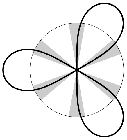
S(m,ε,δ):=⋃k=02​m−1{z∈𝑪∖{0};kmπ+δ−ε<argz<kmπ+δ+ε}.S(m,\varepsilon,\delta):=\bigcup_{k=0}^{2m-1}\left\{z\in\boldsymbol{C}\setminus\{0\}\,;\,\frac{k}{m}\pi+\delta-\varepsilon<\arg z<\frac{k}{m}\pi+\delta+\varepsilon\right\}.
Refer to caption
Figure 3.1. The thick curve is the singular set of Example 3.5 for the case m=3m=3. The shaded parts indicate the set S⁡(3,ε,π/6)S(3,\varepsilon,\pi/6).
Lemma E2.

Suppose f:Δ∗→S13f:\Delta^{*}\to S^{3}_{1} is a gg-regular integral elliptic end. If the singular set accumulates at the end, then there are an m∈𝐙+m\in\boldsymbol{Z}_{+} and a δ∈𝐑\delta\in\boldsymbol{R} such that, for any ε>0\varepsilon>0, there exists an r>0r>0 so that the singular set of ff in {z;0<|z|<r}\{z;0<|z|<r\} lies in S⁡(m,ε,δ)S(m,\varepsilon,\delta).

Proof.

The assertion of the lemma does not depend on a choice of the complex coordinate at the origin.

Since the singular set accumulates at 00, we have |g⁡(0)|=1|g(0)|=1. Then by Proposition 2.2 (1), g⁡(z)g(z) is holomorphic at z=0z=0. Moreover, we may set g⁡(0)=1g(0)=1. Then φ⁡(z):=log⁡g⁡(z)\varphi(z):=\log g(z) is well-defined on a neighborhood of z=0z=0 and φ⁡(0)=0\varphi(0)=0. Using the Weierstrass preparation theorem, we may further assume without loss of generality that φ⁡(z)=zm\varphi(z)=z^{m} for some positive integer mm. Here, |g⁡(z)|=1|g(z)|=1 is equivalent to Re⁡φ⁡(z)=0\operatorname{Re}\varphi(z)=0. Thus, the singular set is expressed as {cosmθ=0}\{\cos m\theta=0\}, where z=r​ei​θz=re^{i\theta}. ∎

Definition 3.6.

A parabolic end of a CMC-11 face is of the first kind if

S⁡(d​σ2)−d​z22​z2=S⁡(g)−d​z22​z2=S⁡(G)+2​Q−d​z22​z2S(d\sigma^{2})-\frac{dz^{2}}{2z^{2}}=S(g)-\frac{dz^{2}}{2z^{2}}=S(G)+2Q-\frac{dz^{2}}{2z^{2}}

has at most a pole of order 11. Otherwise, it is of the second kind.

Lemma P.

Let f:Δ∗→S13f:\Delta^{*}\to S^{3}_{1} be a gg-regular parabolic end. If the end is of the first kind, the singular set does not accumulate at the end. If the end is of the second kind, then the singular set does accumulate at the end. In this case, there exist an m∈𝐙+m\in\boldsymbol{Z}_{+} and a δ\delta (δ∈[0,π/m])(\delta\in[0,\pi/m]) such that, for all ε>0\varepsilon>0, there exists an r>0r>0 so that the singular set of ff in {z;0<|z|<r}\{z;0<|z|<r\} lies in S⁡(m,ε,δ)S(m,\varepsilon,\delta).

Proof.

Let gg be the secondary Gauss map. Since the end is parabolic, the Schwarzian derivative P:=S⁡(g)P:=S(g) determines a PSU1,1\operatorname{PSU}_{1,1}-projective connection of parabolic monodromy. Then by (2) in Proposition 2.2 for ε=−1\varepsilon=-1 and t=πt=\pi, there exists a PSU1,1\operatorname{PSU}_{1,1} lift g0g_{0} such that

h⁡(z)=g^0​(z)+i​log⁡z(g^0​(z)=R⋆g0​(z)=1i​g0​(z)+1g0​(z)−1)h(z)=\hat{g}_{0}(z)+i\log z\qquad\left(\hat{g}_{0}(z)=R\star g_{0}(z)=\frac{1}{i}\frac{g_{0}(z)+1}{g_{0}(z)-1}\right)

is a meromorphic function on Δ∗\Delta^{*}. Here, there exists a matrix A∈SU1,1A\in\operatorname{SU}_{1,1} such that g=A⋆g0g=A\star g_{0} or 1/g=A⋆g01/g=A\star g_{0} holds. Thus, by the SU1,1\operatorname{SU}_{1,1}-ambiguity of the secondary Gauss map, we may assume g=g0g=g_{0} or 1/g01/g_{0}. Moreover, replacing ff with −f-f if necessary (see Remark 1.11), we may assume g=g0g=g_{0} without loss of generality.

Since the end is gg-regular, (2)(ii) of Proposition 2.2 yields that h⁡(z)h(z) is meromorphic at z=0z=0. Thus, we can write

g^​(z)=g^0​(z)=−i​log⁡z+zm​φ​(z)(φ⁡(0)≠0,m∈𝒁),\hat{g}(z)=\hat{g}_{0}(z)=-i\log z+z^{m}\varphi(z)\qquad(\varphi(0)\neq 0,m\in\boldsymbol{Z}),

where φ⁡(z)\varphi(z) is a holomorphic function on a neighborhood of the origin. Then there exist an a∈𝑹∖{0}a\in\boldsymbol{R}\setminus\{0\} and a γ∈(−π,π)\gamma\in(-\pi,\pi) such that

Im⁡g^​(z)=−log⁡r+a​rm​sin⁡(m​θ+γ)+o⁡(rm+1),z=r​ei​θ.\operatorname{Im}\hat{g}(z)=-\log r+a{r^{m}}\sin\bigl(m\theta+\gamma\bigr)+o(r^{m+1}),\quad z=re^{i\theta}.

Here, the singular set {|g|=1}\{|g|=1\} is written as {Img^=0}\{\operatorname{Im}\hat{g}=0\}.

If the end is of the first kind, then m≥0m\geq 0 by (2)(iii) in Proposition 2.2. Therefore, for each fixed θ\theta, the right-hand side approaches ∞\infty as r→0r\to 0, which implies that the singular points do not accumulate at the end.

If the end is of the second kind, then m<0m<0. Therefore, for each fixed θ\theta, the right hand side approaches ∞\infty if a​sin⁡(m​θ+γ)>0a\sin(m\theta+\gamma)>0 and −∞-\infty if a​sin⁡(m​θ+γ)<0a\sin(m\theta+\gamma)<0 as r→0r\to 0, giving solutions of Im⁡g^​(z)=0\operatorname{Im}\hat{g}(z)=0 for sufficiently small rr near the lines sin⁡(m​θ+γ)=0\sin(m\theta+\gamma)=0. This implies the second assertion. ∎

Lemma H.

Let f:Δ∗→S13f:\Delta^{*}\to S^{3}_{1} be a gg-regular hyperbolic end. Then any ray in Δ∗\Delta^{*} emanating from the origin meets the singular set infinitely many times. (See Figure 3.2.)

Remark 3.7.

This intersection property does not depend on the choice of a complex coordinate for a punctured neighborhood of the end.

Proof of Lemma H.

By Proposition 2.2 and an appropriate choice of gg, if we set g^=R⋆g\hat{g}=R\star g, then there is a μ∈𝑹∖{0}\mu\in\boldsymbol{R}\setminus\{0\} such that

h⁡(z):=z−i​μ​g^​(z)h(z):=z^{-i\mu}\hat{g}(z)

is a meromorphic function on Δ∗\Delta^{*}. Since ff is gg-regular, (3)(ii) of Proposition 2.2 implies hh has at most a pole at the origin, and S⁡(g)S(g) has a pole of order exactly 22 at z=0z=0. Thus we can rewrite

g^​(z)=zm+i​μ​φ​(z)(φ⁡(0)≠0,m∈𝒁),\hat{g}(z)=z^{m+i\mu}\varphi(z)\qquad(\varphi(0)\neq 0,m\in\boldsymbol{Z}),

where φ⁡(z)\varphi(z) is a single-valued holomorphic function on Δ=Δ∗∪{0}\Delta=\Delta^{*}\cup\{0\}. Now, we set

w=z​exp⁡(log⁡φm+i​μ),w=z\exp\left(\frac{\log\varphi}{m+i\mu}\right),

which gives a new coordinate ww around the end, now at w=0w=0. Then g^​(w)=wm+i​μ\hat{g}(w)=w^{m+i\mu}. Since g=(g^−i)/(g^+i)g=(\hat{g}-i)/(\hat{g}+i), setting w=r​ei​θw=re^{i\theta}, the singular set is

{w;|g⁡(w)|=1}\displaystyle\{w\,;\,|g(w)|=1\} ={w;Im⁡(g^​(w))=0}\displaystyle=\{w\,;\,\operatorname{Im}(\hat{g}(w))=0\}
={(r,θ)∈(0,1)×(−π,π);μlogr+mθ≡0(modπ)},\displaystyle=\left\{(r,\theta)\in(0,1)\times(-\pi,\pi)\,;\,\mu\log r+m\theta\equiv 0\pmod{\pi}\right\},

that is, r=exp⁡((n​π−m​θ)/μ)r=\exp\bigl((n\pi-m\theta)/\mu\bigr), n∈𝒁n\in\boldsymbol{Z}, which is a log-spiral when m≠0m\neq 0. If m=0m=0, the singular set is a union of infinitely many disjoint circles. In any case, the singular set meets any ray based at w=0w=0 infinitely many times. (See Figure 3.2, left-hand side for the case m=0m=0 and right-hand side for the case m≠0m\neq 0.) ∎

Refer to caption      Refer to caption
g^=w10​i\hat{g}=w^{10i}      g^=w1+10​i\hat{g}=w^{1+10i}
Figure 3.2. The thick curves indicate the singular sets of hyperbolic ends with secondary Gauss map g=R−1⋆g^g=R^{-1}\star\hat{g}, as discussed in Lemma H. The thin lines indicate rays in Δ∗\Delta^{*} emanating from the origin. Here we see that the singular sets intersect rays emanating from the origin infinitely many times.
Corollary 3.8.

The monodromy of a hyperbolic metric on Δ∗\Delta^{*} is either elliptic or parabolic. That is, hyperbolic monodromy never occurs.

Proof.

Suppose that a hyperbolic metric d​σ2d\sigma^{2} on Δ∗\Delta^{*} has hyperbolic monodromy. Let gg be a developing map for d​σ2d\sigma^{2}. The data (g,ω=d​z)(g,\omega=dz) produces an FF as in (1.6), and then the immersion f=F​e3​F∗:Δ∗→S13f=Fe_{3}F^{*}:\Delta^{*}\to S_{1}^{3} is without singularities, since d​σ2d\sigma^{2} is nonsingular. By Theorem 2.6, ff is gg-regular at z=0z=0. Then by Lemma H, the singularities accumulate at the end, a contradiction. ∎

Lemmas E1, E2, P and H imply:

Corollary 3.9 (Characterization of hyperbolic ends).

A gg-regular end f:Δ∗→S13f:\Delta^{*}\to S^{3}_{1} of a CMC-11 face is hyperbolic if and only if every ray in Δ∗\Delta^{*} emanating from the origin meets the singular set infinitely many times.

Completeness

We now give two theorems on complete CMC-11 faces.

Theorem 3.10.

Any complete end of a CMC-11 face is either gg-regular elliptic or gg-regular parabolic of the first kind.

Proof.

By Proposition 1.17, the end is of puncture-type. Moreover, Theorem 2.6 implies the end is gg-regular. Thus the theorem follows from Corollary 3.8 and Lemma P. ∎

Theorem 3.11.

Any complete CMC-11 face is of finite type. ((The definition of finite type is given in Definition 1.16.))

Proof.

Let f:M2→S13f:M^{2}\to S^{3}_{1} be a complete CMC-11 face. Then by Proposition 1.17, there is a compact Riemann surface M¯2\overline{M}^{2} such that MM is biholomorphic to M¯2∖{p1,…,pn}\overline{M}^{2}\setminus\{p_{1},\dots,p_{n}\}.

We fix any end pjp_{j}, and take a small coordinate neighborhood (U,z)(U,z) with z=0z=0 at pjp_{j}. We may assume that there are no singular points on U∖{pj}U\setminus\{p_{j}\}, and thus we may also assume that |g|<1|g|<1 on U∖{pj}U\setminus\{p_{j}\} for a secondary Gauss map gg. We know from Theorem 3.10 that the end is a gg-regular elliptic end or a gg-regular parabolic end of the first kind.

First, we consider the elliptic case. Since |g|<1|g|<1, we may assume that there exist some μ(≥0)\mu(\geq 0) and a holomorphic function h⁡(z)h(z) on UU with h⁡(0)≠0h(0)\neq 0 such that g⁡(z)=zμ​h​(z)g(z)=z^{\mu}h(z). If |g⁡(0)|=1|g(0)|=1, then μ=0\mu=0 and

g⁡(z)=ei​θ​(1+a​zm+o⁡(zm))g(z)=e^{i\theta}\bigl(1+az^{m}+o(z^{m})\bigr)

for some θ∈𝑹\theta\in\boldsymbol{R}, a∈𝑪∖{0}a\in\boldsymbol{C}\setminus\{0\} and m∈𝒁+m\in\boldsymbol{Z}_{+}, which contradicts the fact that |g|<1|g|<1 on U∖{pj}U\setminus\{p_{j}\}. Hence |g⁡(0)|<1|g(0)|<1. Therefore, there exist a neighborhood U~⊂U\widetilde{U}\subset U of pjp_{j} and an ε>0\varepsilon>0 such that |g|2<1−ε|g|^{2}<1-\varepsilon on U~\widetilde{U}. So, on U~\widetilde{U},

(3.1) Kd​s2​d​s2=4​|d​g|2(1−|g|2)2≤4ε2​4​|d​g|2(1+|g|2)2=4ε2​(−Kd​s^2)​d​s^2,K_{ds^{2}}\,ds^{2}=\frac{4|dg|^{2}}{(1-|g|^{2})^{2}}\leq\frac{4}{\varepsilon^{2}}\frac{4\,|dg|^{2}}{(1+|g|^{2})^{2}}=\frac{4}{\varepsilon^{2}}(-K_{d\hat{s}^{2}})\,d\hat{s}^{2},

where d​s^2d\hat{s}^{2} is the metric as in (1.5), which is defined on U~∖{pj}\widetilde{U}\setminus\{p_{j}\} because g⁡(z)=zμ​h​(z)g(z)=z^{\mu}h(z). Since pjp_{j} is a regular singularity of the punctured spherical metric

d​σ^2:=(−Kd​s^2)​d​s^2=4​|d​g|2(1+|g|2)2,d\hat{\sigma}^{2}:=(-K_{d\hat{s}^{2}})\,d\hat{s}^{2}=\frac{4\,|dg|^{2}}{(1+|g|^{2})^{2}},

d​σ^2d\hat{\sigma}^{2} has finite area, so d​s2ds^{2} has finite total curvature on U~∖{pj}\widetilde{U}\setminus\{p_{j}\}, by (3.1).

Next we consider the parabolic case. By Theorem 3.10, the end is parabolic of the first kind. Then without loss of generality, we may assume there exists a holomorphic function h⁡(z)h(z) on Δ\Delta such that (we set t=πt=\pi and replace h⁡(z)h(z) by i​h​(z)ih(z) in the proof of Proposition 2.2)

(3.2) g^​(z)=i⁡(h⁡(z)±log⁡z),whereg^​(z)=R⋆g⁡(z)=1i​g⁡(z)+1g⁡(z)−1.\hat{g}(z)=i(h(z)\pm\log z),\qquad\text{where}\quad\hat{g}(z)=R\star g(z)=\frac{1}{i}\frac{g(z)+1}{g(z)-1}.

If we set k⁡(z):=h⁡(z)±log⁡z+1k(z):=h(z)\pm\log z+1, we have g=1−2/kg=1-2/k, g′=2​k′/k2g^{\prime}=2k^{\prime}/k^{2} and

1−|g⁡(z)|2=4​(Re⁡k​(z)−1)|k⁡(z)|2=4​(Re⁡h​(z)±Re⁡log⁡z)|k⁡(z)|2.1-|g(z)|^{2}=\frac{4(\operatorname{Re}k(z)-1)}{|k(z)|^{2}}=\frac{4(\operatorname{Re}h(z)\pm\operatorname{Re}\log z)}{|k(z)|^{2}}.

So we have

(3.3) d​σ2=4​|d​g|2(1−|g|2)2=|h′​(z)±(1/z)|2​|d​z|2(Re⁡h⁡(z)±Re⁡log⁡z)2.d\sigma^{2}=\frac{4\,|dg|^{2}}{(1-|g|^{2})^{2}}=\frac{|h^{\prime}(z)\pm(1/z)|^{2}|dz|^{2}}{(\operatorname{Re}h(z)\pm\operatorname{Re}\log z)^{2}}.

We set c:=supz∈Δ|Re⁡h⁡(z)|c:=\sup_{z\in\Delta}|\operatorname{Re}h(z)| and r=|z|r=|z|. Since log⁡r→−∞\log r\to-\infty as z→0z\to 0, we may assume −log⁡r>c-\log r>c. Then

|Re⁡h⁡(z)±log⁡r|≥||Re⁡h⁡(z)|−|log⁡r||≥|c+log⁡r|,and|\operatorname{Re}h(z)\pm\log r|\geq\bigl||\operatorname{Re}h(z)|-|\log r|\bigr|\geq|c+\log r|,\quad\text{and}
(3.4) d​σ2≤C2r2​(c+log⁡r)2​|d​z|2,d\sigma^{2}\leq\frac{C^{2}}{r^{2}(c+\log r)^{2}}|dz|^{2},

where C=supz∈Δ|z​h′​(z)+1|C=\sup_{z\in\Delta}|zh^{\prime}(z)+1|. Since

∫0εC2​r​d​rr2​(c+log⁡r)2=−C2c+log⁡ε<∞,\int_{0}^{\varepsilon}\frac{C^{2}r\,dr}{r^{2}(c+\log r)^{2}}=-\frac{C^{2}}{c+\log\varepsilon}<\infty,

the area of a sufficiently small punctured neighborhood of z=0z=0 with respect to d​σ2d\sigma^{2} is finite, which proves the assertion. ∎

Theorem I in the introduction follows from Theorems 3.10 and 3.11.

4. The light-cone Gauss map and
extrinsic behavior of ends

Let 𝐿𝐶={x∈𝑹14;⟨x,x⟩=0}\operatorname{\mathit{LC}}=\{x\in\boldsymbol{R}^{4}_{1}\,;\,\left\langle{x},{x}\right\rangle=0\} be the light-cone of 𝑹14\boldsymbol{R}^{4}_{1}, with future and past light cones

𝐿𝐶±:={x=(x0,x1,x2,x3)∈𝐿𝐶;±x0>0}.\operatorname{\mathit{LC}}_{\pm}:=\{x=(x_{0},x_{1},x_{2},x_{3})\in\operatorname{\mathit{LC}}\,;\,\pm x_{0}>0\}.

The multiplicative group 𝑹+\boldsymbol{R}_{+} of the positive real numbers acts on 𝐿𝐶±\operatorname{\mathit{LC}}_{\pm} by scalar multiplication. The ideal boundary ∂S13\partial S^{3}_{1} of S13S^{3}_{1} consists of two (future and past) components

∂±S13:=𝐿𝐶±/𝑹+,\partial_{\pm}S^{3}_{1}:=\operatorname{\mathit{LC}}_{\pm}/\boldsymbol{R}_{+},

each of which are identified with 𝑪∪{∞}\boldsymbol{C}\cup\{\infty\} by the projection

(4.1) π:∂±S13∋[(v0,v1,v2,v3)]⟼1v0−v3​(v1+i​v2)∈𝑪∪{∞}.\pi\colon\partial_{\pm}S^{3}_{1}\ni\bigl[(v_{0},v_{1},v_{2},v_{3})\bigr]\longmapsto\frac{1}{v_{0}-v_{3}}(v_{1}+iv_{2})\in\boldsymbol{C}\cup\{\infty\}.

The isometries of 𝑹14\boldsymbol{R}^{4}_{1} induce Möbius transformations on 𝑪∪{∞}\boldsymbol{C}\cup\{\infty\}. The boundary ∂S13\partial S^{3}_{1} is identified with the set of equivalence classes of oriented time-like geodesics in S13S^{3}_{1}.

In particular, for a space-like immersion f:M2→S13f\colon{}M^{2}\to S^{3}_{1} with the (time-like) unit normal vector field ν\nu, the equivalence class [f+ν][f+\nu] determines a point in ∂S13\partial S^{3}_{1} for each p∈M2p\in M^{2}. Hence we have the light-cone Gauss map

L=[f+ν]:M2⟶∂S13.L=[f+\nu]\colon{}M^{2}\longrightarrow\partial S^{3}_{1}.

Let f:M2→S13f\colon{}M^{2}\to S^{3}_{1} be a CMC-11 face, and p∈M2p\in M^{2} a regular point, that is, ff is an immersion in a neighborhood of pp. Under the identification of 𝑹14\boldsymbol{R}^{4}_{1} and Herm⁡(2)\operatorname{Herm}(2) as in (1.1), we can compute that the unit normal vector ν\nu is

ν=1|g|2−1​F​(1+|g|22​g2​g¯1+|g|2)​F∗,\nu=\frac{1}{|g|^{2}-1}F\begin{pmatrix}1+|g|^{2}&2g\\ 2\bar{g}&1+|g|^{2}\end{pmatrix}F^{*},

where FF is the holomorphic lift of ff and gg is the secondary Gauss map. Hence

(4.2) L=[2|g|2−1​F​(|g|2gg¯1)​F∗]=sgn⁡(|g|2−1)​[F​(|g|2gg¯1)​F∗],L=\!\left[\frac{2}{|g|^{2}-1}F\begin{pmatrix}|g|^{2}&g\\ \bar{g}&1\end{pmatrix}F^{*}\right]=\operatorname{sgn}(|g|^{2}-1)\!\!\left[F\begin{pmatrix}|g|^{2}&g\\ \bar{g}&1\end{pmatrix}F^{*}\right],

where sgn⁡(|g|2−1)\operatorname{sgn}(|g|^{2}-1) is the sign of the function |g|2−1|g|^{2}-1. Thus, we have:

Proposition 4.1.

The light-cone Gauss map LL of a CMC-11 face takes values in ∂+S13\partial_{+}S^{3}_{1} (resp. ∂−S13\partial_{-}S^{3}_{1}) if |g|>1|g|>1 (resp. |g|<1|g|<1). Moreover, its projection π∘L\pi\circ L is the hyperbolic Gauss map GG as in (1.9), which extends to the singular set.

Proof.

By (4.2), the x0x_{0}-component of f+νf+\nu is

1|g|2−1​trace⁡(F​(|g|2gg¯1)​F∗)=1|g|2−1​(|g​F11+F12|2+|g​F21+F22|2),\frac{1}{|g|^{2}-1}\operatorname{trace}\left(F\begin{pmatrix}|g|^{2}&g\\ \bar{g}&1\end{pmatrix}F^{*}\right)=\frac{1}{|g|^{2}-1}\left(|gF_{11}+F_{12}|^{2}+|gF_{21}+F_{22}|^{2}\right),

where F=(Fi​j)i,j=1,2F=(F_{ij})_{i,j=1,2}. Here, |g​F11+F12|2+|g​F21+F22|2>0|gF_{11}+F_{12}|^{2}+|gF_{21}+F_{22}|^{2}>0 holds because detF=1≠0\det F=1\neq 0, implying the first part of the proposition. By (4.2), (4.1), (1.6) and (1.9), we have

π∘L=π∘[f+ν]=g​F11+F12g​F21+F22=d​F11d​F21=G,\pi\circ L=\pi\circ[f+\nu]=\frac{gF_{11}+F_{12}}{gF_{21}+F_{22}}=\frac{dF_{11}}{dF_{21}}=G,

and this completes the proof. ∎

Next we give a criterion for when a complete regular end approaches ∂+S13\partial_{+}S^{3}_{1} or ∂−S13\partial_{-}S^{3}_{1}:

Proposition 4.2.

Let f:Δ∗→S13f:\Delta^{*}\to S^{3}_{1} be a complete regular end at z=0z=0 and let gg be a secondary Gauss map of ff. Then the image of ff converges to a point in ∂+S13\partial_{+}S^{3}_{1} (resp. ∂−S13\partial_{-}S^{3}_{1}) at the end if and only if |g|<1|g|<1 (resp. |g|>1|g|>1) near the end.

Proof.

We can change the holomorphic null lift FF to F♮F^{\natural} as in (1.14), so that ff and its secondary Gauss map gg change to −f-f and 1/g1/g. The end of ff approaches ∂±S13\partial_{\pm}S^{3}_{1} if and only if −f-f approaches ∂∓S13\partial_{\mp}S^{3}_{1}, so it is sufficient to prove this result under the assumption |g|<1|g|<1 on Δ∗\Delta^{*}. By Theorem 3.10, the end is either elliptic or parabolic.

First we assume the end is elliptic. Replacing FF by a​F​b−1aFb^{-1} (a∈SL2⁡𝑪a\in\operatorname{SL}_{2}\boldsymbol{C}, b∈SU1,1b\in\operatorname{SU}_{1,1}) and using the Weierstrass preparation theorem if necessary, we may assume without loss of generality that the hyperbolic and secondary Gauss maps are

G⁡(z)=zm,g⁡(z)=zμ​h​(z)for some ​m∈𝒁+,μ∈𝑹∖{0},G(z)=z^{m},\qquad g(z)=z^{\mu}h(z)\qquad\text{for some }m\in\boldsymbol{Z}_{+},~\mu\in\boldsymbol{R}\setminus\{0\}\;,

where hh is a holomorphic function on Δ\Delta with h⁡(0)≠0h(0)\neq 0. Here μ>0\mu>0 because |g|<1|g|<1.

If m≠μm\neq\mu, Small’s formula (1.10) implies that

F=12​m​μ​(−zm−μ2​(m+μ)​(1+o⁡(1))zm+μ2​(m−μ)​(1+o⁡(1))z−m−μ2​(m−μ)​(1+o⁡(1))−z−m+μ2​(m+μ)​(1+o⁡(1))).F=\frac{1}{2\sqrt{m\mu}}\begin{pmatrix}-z^{\frac{\hphantom{-}m-\mu}{2}}(m+\mu)\bigl(1+o(1)\bigr)&\hphantom{-}z^{\frac{\hphantom{-}m+\mu}{2}}(m-\mu)\bigl(1+o(1)\bigr)\\ \hphantom{-}z^{\frac{-m-\mu}{2}}(m-\mu)\bigl(1+o(1)\bigr)&-z^{\frac{-m+\mu}{2}}(m+\mu)\bigl(1+o(1)\bigr)\end{pmatrix}.

Since mm and μ\mu are positive, the first component x0x_{0} is

x0=12​trace⁡(F​e3​F∗)=(m−μ)28​m​μ​r−m−μ​(1+o⁡(1))→+∞(r→0),x_{0}=\frac{1}{2}\operatorname{trace}(Fe_{3}F^{*})=\frac{(m-\mu)^{2}}{8m\mu}r^{-m-\mu}\bigl(1+o(1)\bigr)\to+\infty\qquad(r\to 0),

where z=r​ei​θz=re^{i\theta}. Other components of f=(x0,x1,x2,x3)f=(x_{0},x_{1},x_{2},x_{3}) are expressed as

x1+i​x2\displaystyle x_{1}+ix_{2} =ei​m​θ​r−μ​μ2−m24​μ​m​(1+o⁡(1)),\displaystyle=e^{im\theta}r^{-\mu}\frac{\mu^{2}-m^{2}}{4\mu m}\bigl(1+o(1)\bigr),
x3\displaystyle x_{3} =−(m−μ)28​m​μ​r−m−μ​(1+o⁡(1)).\displaystyle=-\frac{(m-\mu)^{2}}{8m\mu}r^{-m-\mu}\bigl(1+o(1)\bigr).

We now consider the stereographic projection given in [F]:

(4.3) Π:{(x0,x1,x2,x3)∈S13;x0>1}∋(x0,x1,x2,x3)⟼11+x0(x1,x2,x3)∈{(X1,X2,X3)∈𝑹3;12<∑j=13(Xj)2<1},\Pi:\{(x_{0},x_{1},x_{2},x_{3})\in S^{3}_{1}\,;\,x_{0}>1\}\ni(x_{0},x_{1},x_{2},x_{3})\\ \longmapsto\frac{1}{1+x_{0}}(x_{1},x_{2},x_{3})\in\left\{(X_{1},X_{2},X_{3})\in\boldsymbol{R}^{3}\,;\,\frac{1}{2}<\sum_{j=1}^{3}(X_{j})^{2}<1\right\},

which is a diffeomorphism. Then Π∘f\Pi\circ f is expressed as

Π∘f=(0,0,−1)+o⁡(1).\Pi\circ f=(0,0,-1)+o(1).

Thus, Π∘f\Pi\circ f approaches (0,0,−1)∈S2=∂+S13(0,0,-1)\in S^{2}=\partial_{+}S_{1}^{3}.

When μ=m\mu=m, by (1.10) again, F11F_{11}, F12F_{12} and F22F_{22} are bounded on a neighborhood of 00, and these components can be extended to become holomorphic on a neighborhood of 00. If F21F_{21} is bounded, FF must be holomorphic and then the induced metric is bounded, which contradicts the weak completeness of the end. Hence F21F_{21} has a pole at 00. So the x0x_{0}-component of ff is

x0=12​|F21|2+(a bounded function)→+∞(z→0).x_{0}=\frac{1}{2}|F_{21}|^{2}+\text{(a bounded function)}\to+\infty\qquad(z\to 0).

Moreover, since

x3\displaystyle x_{3} =−12​|F21|2+(a bounded function),\displaystyle=-\frac{1}{2}|F_{21}|^{2}+\text{(a bounded function)},
x1+i​x2\displaystyle x_{1}+ix_{2} =F11​F21¯−F12​F22¯=c​F21¯+(a bounded function),\displaystyle=F_{11}\overline{F_{21}}-F_{12}\overline{F_{22}}=c\overline{F_{21}}+\text{(a bounded function)},

we have Π∘f→(0,0,−1)\Pi\circ f\to(0,0,-1) as z→0z\to 0.

Next we assume the end is parabolic. Again we may set G=zmG=z^{m}, m∈𝒁+m\in\boldsymbol{Z}_{+}. Applying Proposition 2.2 for t=2​m​πt=2m\pi and ε=−1\varepsilon=-1, there exists a PSU1,1\operatorname{PSU}_{1,1}-lift g0g_{0} of S⁡(g)S(g) such that h⁡(z):=R⋆g0​(z)+2​m​i​log⁡zh(z):=R\star g_{0}(z)+2mi\log z is a single-valued meromorphic function on Δ∗\Delta^{*}, and the secondary Gauss map gg satisfies g=A⋆g0g=A\star g_{0} or 1/g=A⋆g01/g=A\star g_{0} for some A∈SU1,1A\in\operatorname{SU}_{1,1}. By completeness, Lemma P implies that the end is of first kind. Hence by (2)(iii) of Proposition 2.2, h⁡(z)h(z) is holomorphic on a neighborhood of the origin. Moreover, by the assumption |g|<1|g|<1, (2)(iv) of Proposition 2.2 yields that g=A⋆g0g=A\star g_{0} for some A∈SU1,1A\in\operatorname{SU}_{1,1}. Thus, without loss of generality, we may set

R⋆g⁡(z)=2​m​i​(k⁡(z)−log⁡z),R\star g(z)=2mi\bigl(k(z)-\log z\bigr),

here we set h⁡(z)=2​m​i​k​(z)h(z)=2mik(z).

For a holomorphic null lift FF of ff with the secondary Gauss map gg, set

F^=F​B−1,whereB:=((1002​i)​R)=(1/21/2−11)∈SL2⁡𝑪.\hat{F}=FB^{-1},\qquad\text{where}\quad B:=\left(\begin{pmatrix}1&0\\ 0&2i\end{pmatrix}R\right)=\begin{pmatrix}1/2&1/2\\ -1&1\end{pmatrix}\in\operatorname{SL}_{2}\boldsymbol{C}.

Then F^\hat{F} is a holomorphic null immersion whose hyperbolic Gauss map G^\hat{G} and secondary Gauss map g^\hat{g} are given by

(4.4) G^\displaystyle\hat{G} =G=zm,\displaystyle=G=z^{m},
g^​(z)\displaystyle\hat{g}(z) =B⋆g⁡(z)=(1002​i)⋆(R⋆g⁡(z))=m⁡(k⁡(z)−log⁡z).\displaystyle=B\star g(z)=\begin{pmatrix}1&0\\ 0&2i\end{pmatrix}\star\bigl(R\star g(z)\bigr)=m\bigl(k(z)-\log z\bigr).

So applying (1.10) for this (G^,g^)(\hat{G},\hat{g}), the components of F^\hat{F} are written as

(4.5) F^11​(z)\displaystyle\hat{F}_{11}(z) =−i2zm/2φ1(z),\displaystyle=-\frac{i}{2}z^{m/2}\varphi_{1}(z),\qquad F^12​(z)\displaystyle\hat{F}_{12}(z) =−i2​zm/2​(m​φ1​(z)​log⁡z+ψ1​(z)),\displaystyle=-\frac{i}{2}z^{m/2}\bigl(m\varphi_{1}(z)\log z+\psi_{1}(z)\bigr),
F^21​(z)\displaystyle\hat{F}_{21}(z) =i2z−m/2φ2(z),\displaystyle=\frac{i}{2}z^{-m/2}\varphi_{2}(z),\qquad F^22​(z)\displaystyle\hat{F}_{22}(z) =i2z−m/2(mφ2(z)logz+ψ2(z)),\displaystyle=\frac{i}{2}z^{-m/2}\bigl(m\varphi_{2}(z)\log z+\psi_{2}(z)\bigr),

where φ1\varphi_{1}, φ2\varphi_{2}, ψ1\psi_{1} and ψ2\psi_{2} are holomorphic functions defined on a neighborhood of the origin such that

φ1​(0)=φ2​(0)=1.\varphi_{1}(0)=\varphi_{2}(0)=1.

Since B​e3​B∗=−e1Be_{3}B^{*}=-e_{1}, f=F​e3​F∗f=Fe_{3}F^{*} satisfies

(4.6) f=−F^​(0110)​F^∗=−(F^11​F^12¯+F^12​F^11¯F^11​F^22¯+F^12​F^21¯F^11¯​F^22+F^12¯​F^21F^21​F^22¯+F^22​F^21¯).f=-\hat{F}\begin{pmatrix}0&1\\ 1&0\end{pmatrix}\hat{F}^{*}=-\begin{pmatrix}\hat{F}_{11}\overline{\hat{F}_{12}}+\hat{F}_{12}\overline{\hat{F}_{11}}&\hat{F}_{11}\overline{\hat{F}_{22}}+\hat{F}_{12}\overline{\hat{F}_{21}}\\ \overline{\hat{F}_{11}}{\hat{F}_{22}}+\overline{\hat{F}_{12}}{\hat{F}_{21}}&\hat{F}_{21}\overline{\hat{F}_{22}}+\hat{F}_{22}\overline{\hat{F}_{21}}\end{pmatrix}.

Hence the components of ff are expressed as

(4.7) x0\displaystyle x_{0} =m4​r−m​(η1​(u,v)​log⁡r+δ1​(u,v)),\displaystyle=\hphantom{-}\frac{m}{4}r^{-m}\bigl(\hphantom{-}\eta_{1}(u,v)\log r+\delta_{1}(u,v)\bigr),
x3\displaystyle x_{3} =m4​r−m​(−η2​(u,v)​log⁡r+δ2​(u,v)),\displaystyle=\hphantom{-}\frac{m}{4}r^{-m}\bigl(-\eta_{2}(u,v)\log r+\delta_{2}(u,v)\bigr),
x1+i​x2\displaystyle x_{1}+ix_{2} =−m2​ei​m​θ​(η3​(u,v)​log⁡r+δ3​(u,v)),\displaystyle=-\frac{m}{2}e^{im\theta}\bigl(\hphantom{-}\eta_{3}(u,v)\log r+\delta_{3}(u,v)\bigr),

where z=r​ei​θ=u+i​vz=re^{i\theta}=u+iv. Here, ηj​(u,v)\eta_{j}(u,v) (j=1,2j=1,2) and δj​(u,v)\delta_{j}(u,v) (j=1,2j=1,2) (resp. η3​(u,v)\eta_{3}(u,v) and δ3​(u,v)\delta_{3}(u,v)) are real-valued (resp. complex-valued) differentiable functions defined on a neighborhood of the origin, such that ηj​(0,0)=1\eta_{j}(0,0)=1 (j=1,2,3j=1,2,3).

The equations (4.7) yield that x0→+∞x_{0}\to+\infty and Π∘f→(0,0,−1)\Pi\circ f\to(0,0,-1) as z→0z\to 0. ∎

5. The Osserman type inequality

Here we prove Theorem II stated in the Introduction. First we prepare:

Lemma 5.1.

The Hopf differential of a CMC-11 face has a pole of order 22 at any complete regular parabolic end.

Proof.

Let f:Δ∗→S13f:\Delta^{*}\to S^{3}_{1} be a complete regular parabolic end at z=0z=0. By Theorem 3.10, the end is of the first kind. Then

2​Q+Sz​(G)​d​z2=Sz​(g)​d​z2=1z2​(12+o⁡(1))​d​z2.2Q+S_{z}(G)\,dz^{2}=S_{z}(g)\,dz^{2}=\frac{1}{z^{2}}\left(\frac{1}{2}+o(1)\right)\,dz^{2}.

Since GG is meromorphic at z=0z=0, we may assume that G=zm​φ​(z)G=z^{m}\varphi(z), where mm is a positive integer and φ⁡(z)\varphi(z) is a holomorphic function on a neighborhood of 00 with φ⁡(0)≠0\varphi(0)\neq 0. Applying (1.19) to Sz​(G)S_{z}(G), it follows that QQ has a pole of order 22 at z=0z=0. ∎

The next lemma improves a result in [F, Proposition 4.4]:

Lemma 5.2.

Let f:Δ∗→S13f:\Delta^{*}\to S^{3}_{1} be a complete regular end at z=0z=0 of a CMC-11 face with Hopf differential QQ and hyperbolic Gauss map GG. Then the ramification order mm of G⁡(z)G(z) at z=0z=0 satisfies

(5.1) m≥Ordz=0(Q)+3.m\geq\operatornamewithlimits{Ord}_{z=0}(Q)+3\;.

(For the definition of the ramification order, see the subsection about the Schwarzian derivative in Section 1.) Here, Ordz=0Q\operatornamewithlimits{Ord}_{z=0}Q denotes the order of QQ at the origin, that is, Ordz=0Q=k\operatornamewithlimits{Ord}_{z=0}Q=k if Q=zk​φ​(z)​d​z2Q=z^{k}\varphi(z)\,dz^{2}, where φ⁡(z)\varphi(z) is holomorphic at z=0z=0 and φ⁡(0)≠0\varphi(0)\neq 0.

Proof.

By Theorem 3.10, a complete end is either elliptic or parabolic of the first kind. The elliptic case has been proved in [F]. Assume that the end is parabolic. Then by Lemma 5.1, QQ must have a pole of order 22 at z=0z=0, which proves the inequality since m≥1m\geq 1. ∎

It should be remarked that the order of the metric d​σ#2=4​|d​G|2/(1+|G|2)2d\sigma^{2}_{\#}=4|dG|^{2}/(1+|G|^{2})^{2} at 00 is equal to m−1m-1, where mm is the ramification order of GG. Using Lemma 5.2 instead of [F, Proposition 4.4], the inequality in Theorem II is proved in the same way as [UY3], [F].

The condition for equality in ( ∗ ‣ II) in Theorem II for elliptic ends was completely analyzed in [F]. So, it suffices to show the following theorem for parabolic ends. Note that Ordp(Q)=−2\operatornamewithlimits{Ord}_{p}(Q)=-2 for complete regular parabolic ends, hence the equality in (5.1) holds if and only if GG does not branch at pp (see [F] for details).

Theorem 5.3.

A complete regular parabolic end of a CMC-11 face is properly embedded if and only if the hyperbolic Gauss map GG does not branch at the end.

Proof.

Let f:Δ∗→S13f:\Delta^{*}\to S^{3}_{1} be a complete regular parabolic end at z=0z=0. Taking −f-f instead of ff if necessary, we may assume that |g|<1|g|<1 in a neighborhood of the end, and that G⁡(z)=zm,m≥1G(z)=z^{m},m\geq 1 and g⁡(z)=R−1⋆(2​m​i​(k⁡(z)−log⁡z))g(z)=R^{-1}\star\left(2mi(k(z)-\log z)\right), as in the proof of Proposition 4.2. Then ff is represented as in (4.5) and (4.6).

By Proposition 4.2, the image of ff tends to a point in ∂+S13\partial_{+}S^{3}_{1}. So we may assume that x0>1x_{0}>1 on Δ∗\Delta^{*}, and

Π∘f:Δ∗∋z⟼(X1,X2,X3)∈𝑹3\Pi\circ f\colon{}\Delta^{*}\ni z\longmapsto(X_{1},X_{2},X_{3})\in\boldsymbol{R}^{3}

is well-defined, where Π\Pi is the projection in (4.3).

Here, by (4.7),

U⁡(z):=z−m​x1+i​x21+x0(=z−m​(X1+i​X2))=−2​η3​log⁡r+δ3η1​log⁡r+δ1+(4/m)​rm.U(z):=z^{-m}\frac{x_{1}+ix_{2}}{1+x_{0}}\left(\vphantom{\int}=z^{-m}(X_{1}+iX_{2})\right)=-2\frac{\eta_{3}\log r+\delta_{3}}{\eta_{1}\log r+\delta_{1}+(4/m)r^{m}}.

Since η1,η3\eta_{1},\eta_{3} and δ1,δ3\delta_{1},\delta_{3} are differentiable functions defined on a neighborhood of 00, we have

(5.2) limz→0U⁡(z)=−2≠0,limz→0z​∂∂z​U​(z)=0​and​limz→0z​∂∂z¯​U​(z)=0.\lim_{z\to 0}U(z)=-2\neq 0,\;\;\lim_{z\to 0}z\frac{\partial}{\partial z}U(z)=0\;\;\text{and}\;\;\lim_{z\to 0}z\frac{\partial}{\partial\bar{z}}U(z)=0.

Now we suppose that the ramification order mm of the hyperbolic Gauss map at z=0z=0 is 11, that is m=1m=1. As seen in the proof of Proposition 4.2, Π∘f\Pi\circ f converges to (0,0,−1)(0,0,-1). Then X1+i​X2=z​U​(z)X_{1}+iX_{2}=zU(z) and (5.2) yield that

limz→0∂∂z​(X1+i​X2)≠0andlimz→0∂∂z¯​(X1+i​X2)=0,\lim_{z\to 0}\frac{\partial}{\partial z}(X_{1}+iX_{2})\neq 0\qquad\text{and}\qquad\lim_{z\to 0}\frac{\partial}{\partial\bar{z}}(X_{1}+iX_{2})=0\;,

which implies that the correspondence z↦X1+i​X2z\mapsto X_{1}+iX_{2} is bijective near the origin, and the end is properly embedded.

Conversely, suppose that the end is properly embedded. We have already seen that X3→−1X_{3}\to-1 as z→0z\to 0. Moreover U⁡(0)≠0U(0)\neq 0 implies that for any sufficiently small ε>0\varepsilon>0, the image of the end f({z;0<|z|<ε})f(\{z;0<|z|<\varepsilon\}) does not meet the X3X_{3}-axis and is diffeomorphic to a cylinder. Then the image of Π∘f⁡({z;|z|=ε})\Pi\circ f(\{z;|z|=\varepsilon\}) by the orthogonal projection (X1,X2,X3)↦X1+i​X2(X_{1},X_{2},X_{3})\mapsto X_{1}+iX_{2} is an embedded closed curve with the winding number mm with respect to the origin. So m=1m=1. ∎

Remark 5.4.

In Proposition 4.4 of [F], the first author showed the equality condition in Theorem II for elliptic ends using the expression of the solution of the ordinary differential equation (1.6). Here we proved the equality condition in Theorem II for parabolic ends by using Small’s formula (1.10). It is also possible to prove the result in [F] more directly by using (1.10).

We give here three important examples:

Example 5.5 (An incomplete 3-noid not satisfying ( ∗ ‣ II) in Theorem II).

We set M2:=𝑪∖{0,1}M^{2}:=\boldsymbol{C}\setminus\{0,1\} and

G:=z,g:=2​z−12​z​(z−1)−log⁡zz−1.G:=z,\qquad g:=\frac{2z-1}{2z(z-1)}-\log\frac{z}{z-1}\;.

Then (1.10) gives a CMC-11 face f:M2→S13f:M^{2}\to S^{3}_{1} with hyperbolic and secondary Gauss maps GG and gg, and Hopf differential

Q=12​(S⁡(g)−S⁡(G))=−2​d​z2z⁡(z−1).Q=\frac{1}{2}(S(g)-S(G))=-\frac{2dz^{2}}{z(z-1)}.

Since the lift metric

d​s#2=4​(1+|z|2)2|z⁡(z−1)|2​|d​z|2ds^{2}_{\#}=\frac{4(1+|z|^{2})^{2}}{|z(z-1)|^{2}}|dz|^{2}

is complete on M2M^{2}, ff is weakly complete. The end z=∞z=\infty is complete and elliptic, and z=0,1z=0,1 are parabolic ends of the second kind. Hence z=0,1z=0,1 are incomplete ends. Since deg⁡(G)=1\deg(G)=1, ff does not satisfy ( ∗ ‣ II). This implies that completeness is an essential assumption in Theorem II in the introduction.

Example 5.6 (A 2-noid with complete parabolic ends satisfying the equality in ( ∗ ‣ II)).

We set

(5.3) F⁡(z)=i2​2​(z00z−1)​(3−log⁡z−1+log⁡z1+log⁡z−3−log⁡z).F(z)=\dfrac{i}{2\sqrt{2}}\begin{pmatrix}\sqrt{z}&0\\ 0&\sqrt{z}^{-1}\end{pmatrix}\!\begin{pmatrix}3-\log z&-1+\log z\\ 1+\log z&-3-\log z\end{pmatrix}.

Then f=F​e3​F∗:𝑪∖{0}→S13f=Fe_{3}F^{*}:\boldsymbol{C}\setminus\{0\}\to S^{3}_{1} has two parabolic regular ends. The hyperbolic Gauss map GG, the secondary Gauss map gg and the Hopf differential QQ are computed as follows:

G=z,g=log⁡z+1log⁡z−1,Q=d​z24​z2.G=z,\qquad g=\frac{\log z+1}{\log z-1},\qquad Q=\frac{dz^{2}}{4z^{2}}.

Since {z∈𝑪;|g⁡(z)|=1}={z∈𝑪;|z|=1}\{z\in\boldsymbol{C}\,;\,|g(z)|=1\}=\{z\in\boldsymbol{C}\,;\,|z|=1\}, the singular set is compact, and hence ff is complete.

Any genus zero CMC-11 face with two parabolic regular ends and with degree 11 hyperbolic Gauss map is congruent to this ff. We call this CMC-11 face the parabolic catenoid. On the other hand, the CMC-11 face with G=zG=z, g=zμg=z^{\mu} (μ∈𝑹∖{0}\mu\in\boldsymbol{R}\setminus\{0\}) given in [F, Example 5.4] is called the elliptic catenoid.

Example 5.7.

(A complete 4-noid with 4 integral elliptic ends satisfying the equality in ( ∗ ‣ II))

Since SL2⁡𝑪\operatorname{SL}_{2}\boldsymbol{C} can be identified with the complex hyperquadric Q3Q^{3} of 𝑪4\boldsymbol{C}^{4}, the null (meromorphic) curves in SL2⁡𝑪\operatorname{SL}_{2}\boldsymbol{C} can be identified with those in Q3Q^{3}. The null curve in SL2⁡𝑪\operatorname{SL}_{2}\boldsymbol{C} with

G:=3​(z3+2)4−z,g:=−z3−12​z2+23​zG:=\frac{3(z^{3}+2)}{4-z},\qquad g:=-\frac{z^{3}-12z^{2}+2}{3z}

belongs to the moduli space ℳ4\mathscr{M}_{4} in the classification list of null curves in Q3Q^{3} in Bryant [B2], which has four integral elliptic ends at the roots of 1+6​z2−z31+6z^{2}-z^{3} and z=∞z=\infty. Since GG is of degree 33 and χ⁡(𝑪∪{∞})=2\chi(\boldsymbol{C}\cup\{\infty\})=2, the corresponding CMC-11 face attains equality in ( ∗ ‣ II) of Theorem II. (For the definition of an integral elliptic end, see Definition 3.4.)

Remark 5.8.

We can deform an elliptic catenoid to a parabolic catenoid. Let fμf_{\mu} be an elliptic catenoid with the hyperbolic Gauss map G=zG=z and the secondary Gauss map g=zμg=z^{\mu}, where μ>0\mu>0. Then the hyperbolic metric corresponding to fμf_{\mu} is

d​σμ2=4​|d​g|2(1−|g|2)2=4​μ2​|z|2​μ−2(1−|z|2​μ)2​|d​z|2.d\sigma_{\mu}^{2}=\frac{4|dg|^{2}}{(1-|g|^{2})^{2}}=\frac{4\mu^{2}|z|^{2\mu-2}}{(1-|z|^{2\mu})^{2}}|dz|^{2}\;.

It can be easily checked that

limμ→0d​σμ2=|d​z|2(r​log⁡r)2,wherez=r​ei​θ,\lim_{\mu\to 0}d\sigma^{2}_{\mu}=\frac{|dz|^{2}}{(r\log r)^{2}},\quad\text{where}\quad z=re^{i\theta},

which is the hyperbolic metric of a parabolic catenoid with

g⁡(z)=R⋆log⁡z=1i​log⁡z+1log⁡z−1,g(z)=R\star\log z=\frac{1}{i}\frac{\log z+1}{\log z-1},

see (3.3). On the other hand, by Small’s formula (1.10) there exists a unique smooth 11-parameter family of CMC-11 faces f~μ\tilde{f}_{\mu} (μ≥0\mu\geq 0) with hyperbolic Gauss map G=zG=z and associated hyperbolic metric d​σμ2d\sigma^{2}_{\mu}. Then f~μ\tilde{f}_{\mu} is congruent to fμf_{\mu}, and f~0\tilde{f}_{0} gives a parabolic catenoid.

Remark 5.9.

As a consequence of Remark 1.21, we know that there are no compact CMC-11 immersed surfaces in S13S^{3}_{1}. Here we give an alternative proof of this: Let M2M^{2} be a compact Riemann surface without boundary, and suppose there exists a compact CMC-11 face f:M2→S13f:M^{2}\to S^{3}_{1} which has no singular points. Let FF be a holomorphic lift of ff. We may assume that |g|<1|g|<1 since there are no singular points. Then, by (1.6), we have

fz​z¯=(1−|g|2)​F​(g1)​(g¯1)​F∗​|ω^|2,f_{z\bar{z}}=(1-|g|^{2})F\begin{pmatrix}g\\ 1\end{pmatrix}\begin{pmatrix}\bar{g}&1\end{pmatrix}F^{*}|\hat{\omega}|^{2},

where zz is a local complex coordinate and ω=ω^​d​z\omega=\hat{\omega}\,dz. Thus, trace⁡f\operatorname{trace}f is a nonconstant subharmonic function, which is a contradiction to the maximum principle.

This proof does not apply to compact CMC-11 faces, leading us to the following open problem:

Problem.

Is there a compact CMC-11 face?

If such a CMC-11 face exists, the genus γ\gamma must be greater than or equal to 33, since equality in ( ∗ ‣ II) in the introduction holds in this case and the degree of the hyperbolic Gauss map must be γ−1\gamma-1.

Appendix A Meromorphicity of the Hopf differential

In this appendix, we shall give a proof of the following

Theorem A.1.

Let M¯2\overline{M}^{2} be a compact Riemann surface. Then the Hopf differential QQ of a complete CMC-11 face

f:M¯2∖{p1,…,pn}⟶S13f\colon{}\overline{M}^{2}\setminus\{p_{1},\dots,p_{n}\}\longrightarrow S^{3}_{1}

is meromorphic on M¯2\overline{M}^{2}.

Proof.

It is sufficient to show the meromorphicity of QQ at a complete end f:Δ∗={z;0<|z|<1}→S13f\colon{}\Delta^{*}=\{z;0<|z|<1\}\to S^{3}_{1} at the origin. We write the Hopf differential QQ as

Q=Q^​d​z2,Q=\hat{Q}\,dz^{2},

where Q^\hat{Q} is a holomorphic function on Δ∗\Delta^{*}. By Theorem 3.10, a complete end f:Δ∗→S13f\colon{}\Delta^{*}\to S^{3}_{1} is either a gg-regular elliptic end or a gg-regular parabolic end of the first kind. (The definition of gg-regularity is given in Definition 3.2.)

First, we consider the case that ff is elliptic. By gg-regularity, the secondary Gauss map is written in the form

g=zμ​h​(z)(h is a holomorphic function with h⁡(0)≠0),g=z^{\mu}h(z)\qquad(\text{$h$ is a holomorphic function with $h(0)\neq 0$}),

where μ\mu is a real number. Since |g⁡(0)|≠1|g(0)|\neq 1 by completeness, we may set g⁡(0)=0g(0)=0, or ∞\infty, because of the SU1,1\operatorname{SU}_{1,1}-ambiguity of gg. Moreover, replacing ff by −f-f if necessary, we may assume μ>0\mu>0 without loss of generality. In this case, the corresponding hyperbolic metric d​σ2d\sigma^{2} is written as

dσ2=(2​|z|μ−1​|μ​h​(z)+z​h′​(z)||1−|z|2​μ​|h⁡(z)|2||dz|)2,(=′dd​z).d\sigma^{2}=\left(\frac{2|z|^{\mu-1}|\mu h(z)+zh^{\prime}(z)|}{\bigl|1-|z|^{2\mu}|h(z)|^{2}\bigr|}\,|dz|\right)^{2},\qquad\left({~}{}^{\prime}=\frac{d}{dz}\right).

Since |z|μ​|h⁡(z)||z|^{\mu}|h(z)| and z​h′​(z)zh^{\prime}(z) tend to 00 as z→0z\to 0 and h⁡(z)h(z) is bounded near the origin, we have that

d​σ≥c​|z|μ−1​|d​z|≥c​|z|l​|d​z|d\sigma\geq c|z|^{\mu-1}\,|dz|\geq c|z|^{l}\,|dz|

holds on a neighborhood of the origin, where ll is the smallest integer such that l≥μ−1l\geq\mu-1 and cc is a positive constant. Then, by (1.16), we have

d​s=2​|Q|d​σ≤2​|Q^|c​|z|l​|d​z|=2c​|Q^zl​d​z|.ds=2\frac{|Q|}{d\sigma}\leq 2\frac{|\hat{Q}|}{c|z|^{l}}|dz|=\frac{2}{c}\left|\frac{\hat{Q}}{z^{l}}\,dz\right|.

Since d​sds is complete at 00, we have meromorphicity of the one-form z−l​Q^​d​zz^{-l}\hat{Q}\,dz at the origin, because of [O, Lemma 9.6, page 83].

Next, we consider the case that ff is parabolic. Since the end is gg-regular parabolic of the first kind, one can choose the secondary Gauss map gg as in (3.2):

g=R−1​g^,g^​(z)=i⁡(h⁡(z)±log⁡z),g=R^{-1}\hat{g},\qquad\hat{g}(z)=i(h(z)\pm\log z),

where h⁡(z)h(z) is a holomorphic function on Δ:=Δ∗∪{0}\Delta:=\Delta^{*}\cup\{0\}. Hence d​σ2d\sigma^{2} is written as in (3.3):

dσ2=(|h′​(z)±(1/z)||Re⁡h⁡(z)±log⁡|z|||dz|)2(=′dd​z).d\sigma^{2}=\left(\frac{|h^{\prime}(z)\pm(1/z)|}{\bigl|\operatorname{Re}h(z)\pm\log|z|\bigr|}\,|dz|\right)^{2}\qquad\left({~}{}^{\prime}=\frac{d}{dz}\right).

Since z​log⁡|z|→0z\log|z|\to 0 as z→0z\to 0 and hh is bounded on a neighborhood of the origin,

d​σ=|1±z​h′​(z)||z​log⁡|z||​|1±Re⁡h⁡(z)log⁡|z||​|d​z|≥c​|d​z|d\sigma=\frac{|1\pm zh^{\prime}(z)|}{\bigl|z\log|z|\bigr|\left|1\pm\frac{\operatorname{Re}h(z)}{\log|z|}\right|}\,|dz|\geq c|dz|

holds on a neighborhood of the origin, where cc is a positive constant. Thus,

d​s=2​|Q|d​σ≤2c​|Q^​d​z|.ds=2\frac{|Q|}{d\sigma}\leq\frac{2}{c}|\hat{Q}\,dz|.

Hence, by the same argument as in the elliptic case, we have meromorphicity of QQ at the origin. ∎

Appendix B Conjugacy classes of SU1,1\operatorname{SU}_{1,1}

The Lie group SU1,1\operatorname{SU}_{1,1} is the set of matrices S∈SL2⁡𝑪S\in\operatorname{SL}_{2}\boldsymbol{C} satisfying S​e3​S∗=e3Se_{3}S^{*}=e_{3}. Two matrices A,B∈SU1,1A,B\in\operatorname{SU}_{1,1} are called conjugate in SL2⁡𝑪\operatorname{SL}_{2}\boldsymbol{C} if there exists a matrix P∈SL2⁡𝑪P\in\operatorname{SL}_{2}\boldsymbol{C} such that B=P−1​A​PB=P^{-1}AP, and are called conjugate in SU1,1\operatorname{SU}_{1,1} if B=P−1​A​PB=P^{-1}AP for some P∈SU1,1P\in\operatorname{SU}_{1,1}.

As in (1.18) and (2.2), we set

Λe​(t)\displaystyle\Lambda_{e}(t) :=(ei​t00e−i​t),\displaystyle:=\begin{pmatrix}e^{it}&0\\ 0&e^{-it}\end{pmatrix},\qquad Λp​(t)\displaystyle\Lambda_{p}(t) :=(1+i​t−i​ti​t1−i​t),\displaystyle:=\begin{pmatrix}1+it&-it\\ it&1-it\end{pmatrix},
Λh​(t)\displaystyle\Lambda_{h}(t) :=(cosh⁡tsinh⁡tsinh⁡tcosh⁡t)\displaystyle:=\begin{pmatrix}\cosh t&\sinh t\\ \sinh t&\cosh t\end{pmatrix}\quad andR\displaystyle\quad\text{and}\quad R :=12​(11i−i)\displaystyle:=\frac{1}{2}\begin{pmatrix}1&\hphantom{-}1\\ i&-i\end{pmatrix}

for an arbitrary t∈𝑹t\in\boldsymbol{R}.

Theorem B.1.

A matrix A∈SU1,1A\in\operatorname{SU}_{1,1} is conjugate in SU1,1\operatorname{SU}_{1,1} to one of

  1. (1)

    Λe​(s)\Lambda_{e}(s) (s∈(−π,π])(s\in(-\pi,\pi]),

  2. (2)

    ±Λp​(t)\pm\Lambda_{p}(t) or ±Λp​(−t)\pm\Lambda_{p}(-t) (t>0)(t>0), or

  3. (3)

    ±Λh​(t)\pm\Lambda_{h}(t) (t>0)(t>0).

Remark B.2.

Though the matrices Λe​(s)\Lambda_{e}(s) and Λe​(−s)\Lambda_{e}(-s) are conjugate in SL2⁡𝑪\operatorname{SL}_{2}\boldsymbol{C}, they are not conjugate in SU1,1\operatorname{SU}_{1,1} if s≢0(mod2​π)s\not\equiv 0\pmod{2\pi}. That is, for any elliptic matrix A∈SU1,1A\in\operatorname{SU}_{1,1}, there exists a unique real number t∈(−π,π]t\in(-\pi,\pi] such that AA and Λe​(s)\Lambda_{e}(s) are conjugate in SU1,1\operatorname{SU}_{1,1}.

Remark B.3.

On the other hand, Λp​(t1)\Lambda_{p}(t_{1}) and Λp​(t2)\Lambda_{p}(t_{2}) (t1,t2≠0t_{1},t_{2}\neq 0) are conjugate in SU1,1\operatorname{SU}_{1,1} if and only if t1​t2>0t_{1}t_{2}>0. In fact, if t1≠t2t_{1}\neq t_{2}, P​Λp​(t1)​P−1=Λp​(t2)P\Lambda_{p}(t_{1})P^{-1}=\Lambda_{p}(t_{2}) (P∈SU1,1P\in\operatorname{SU}_{1,1}) holds if and only if

P=±(ab¯ba¯),a=cosh⁡s+i​u,b=sinh⁡s+i​u,P=\pm\begin{pmatrix}a&\bar{b}\\ b&\bar{a}\end{pmatrix},\qquad a=\cosh s+iu,~b=\sinh s+iu,

where s=log⁡t2/t1∈𝑹s=\log\sqrt{t_{2}/t_{1}}\in\boldsymbol{R} and u∈𝑹u\in\boldsymbol{R}.

In particular, the sign of tt in Λp​(t)\Lambda_{p}(t) is invariant under such a conjugation. Though Λp​(t)\Lambda_{p}(t) (t∈𝑹∖{0}t\in\boldsymbol{R}\setminus\{0\}) is conjugate with Λp​(1)\Lambda_{p}(1) or Λp​(−1)\Lambda_{p}(-1), we choose various values of tt in this paper for the sake of convenience.

Remark B.4.

Since

(i00−i)​(cosh⁡tsinh⁡tsinh⁡tcosh⁡t)​(−i00i)=(cosh⁡t−sinh⁡t−sinh⁡tcosh⁡t)\begin{pmatrix}i&\hphantom{-}0\\ 0&-i\end{pmatrix}\begin{pmatrix}\cosh t&\sinh t\\ \sinh t&\cosh t\end{pmatrix}\begin{pmatrix}-i&0\\ \hphantom{-}0&i\end{pmatrix}=\begin{pmatrix}\cosh t&-\sinh t\\ -\sinh t&\cosh t\end{pmatrix}

Λh​(t)\Lambda_{h}(t) and Λh​(−t)\Lambda_{h}(-t) are conjugate in SU1,1\operatorname{SU}_{1,1}.

To show Theorem B.1, we use the following group isomorphism:

ρ:SL2⁡𝑹∋X⟼R−1​X​R∈SU1,1.\rho\colon{}\operatorname{SL}_{2}\boldsymbol{R}\ni X\longmapsto R^{-1}XR\in\operatorname{SU}_{1,1}.

Note that Λe​(t),Λp​(t)\Lambda_{e}(t),\Lambda_{p}(t), and Λh​(t)\Lambda_{h}(t) are the images of

(cos⁡tsin⁡t−sin⁡tcos⁡t),(12​t01),and(et00e−t)\begin{pmatrix}\hphantom{-}\cos t&\sin t\\ -\sin t&\cos t\end{pmatrix},\quad\begin{pmatrix}1&2t\\ 0&1\end{pmatrix},\quad\text{and}\quad\begin{pmatrix}e^{t}&0\\ 0&e^{-t}\end{pmatrix}

respectively, by ρ\rho.

Lemma B.5.

Let AA and BB be 2×22\times 2 real matrices that are conjugate in SL2⁡𝐂\operatorname{SL}_{2}\boldsymbol{C}. Then AA and either BB or e3​B​e3e_{3}Be_{3} are conjugate in SL2⁡𝐑\operatorname{SL}_{2}\boldsymbol{R}.

Proof.

By assumption, there is a P~∈SL2⁡𝑪\widetilde{P}\in\operatorname{SL}_{2}\boldsymbol{C} with A​P~=P~​BA\widetilde{P}=\widetilde{P}B. We set P~=U+i​V\widetilde{P}=U+iV, for real matrices UU, VV. Then A​U=U​BAU=UB, A​V=V​BAV=VB and

A⁡(U+t​V)=(U+t​V)​Bfor any ​t∈𝑹.A(U+tV)=(U+tV)B\qquad\text{for any }t\in\boldsymbol{R}.

If det(U+t​V)\det(U+tV) vanishes identically for all t∈𝑹t\in\boldsymbol{R}, holomorphicity of 𝑪∋t↦det(U+t​V)\boldsymbol{C}\ni t\mapsto\det(U+tV) yields that det(U+i​V)=detP~=0\det(U+iV)=\det\widetilde{P}=0, a contradiction. Thus for some t0∈𝑹t_{0}\in\boldsymbol{R}, det(U+t0​V)≠0\det(U+t_{0}V)\neq 0, and then (U+t0​V)−1​A​(U+t0​V)=B(U+t_{0}V)^{-1}A(U+t_{0}V)=B. If det(U+t0​V)>0\det(U+t_{0}V)>0, we set P=(U+t0​V)/det(U+t0​V)∈SL2⁡𝑹P=(U+t_{0}V)/\sqrt{\det(U+t_{0}V)}\in\operatorname{SL}_{2}\boldsymbol{R}, giving P−1​A​P=BP^{-1}AP=B. If det(U+t0​V)<0\det(U+t_{0}V)<0, we set P=(U+t0​V)​e3/|det(U+t0​V)|∈SL2⁡𝑹P=(U+t_{0}V)e_{3}/\sqrt{|\det(U+t_{0}V)|}\in\operatorname{SL}_{2}\boldsymbol{R}, giving P−1​A​P=e3​B​e3P^{-1}AP=e_{3}Be_{3}. ∎

Proof of Theorem B.1.

Let A∈SU1,1A\in\operatorname{SU}_{1,1} and A~:=ρ−1​(A)∈SL2⁡𝑹\widetilde{A}:=\rho^{-1}(A)\in\operatorname{SL}_{2}\boldsymbol{R}.

If the eigenvalues of AA are not real numbers, they are written as {ei​t,e−i​t}\{e^{it},e^{-it}\}, where t∈(−π,0)∪(0,π)t\in(-\pi,0)\cup(0,\pi). In this case, A~\widetilde{A} is conjugate in SL2⁡𝑪\operatorname{SL}_{2}\boldsymbol{C} to Be:=R​Λe​(t)​R−1B_{e}:=R\Lambda_{e}(t)R^{-1}. Hence by Lemma B.5, A~\widetilde{A} is conjugate in SL2⁡𝑹\operatorname{SL}_{2}\boldsymbol{R} to BeB_{e} or e3​Be​e3e_{3}B_{e}e_{3}. Thus, A=ρ⁡(A~)A=\rho(\widetilde{A}) is conjugate in SU1,1\operatorname{SU}_{1,1} to ρ⁡(Be)=Λe​(t)\rho(B_{e})=\Lambda_{e}(t) or ρ⁡(e3​Be​e3)=Λe​(−t)\rho(e_{3}B_{e}e_{3})=\Lambda_{e}(-t).

If the eigenvalues of AA are {ε,ε}\{\varepsilon,\varepsilon\} (ε={−1,1}\varepsilon=\{-1,1\}) and A≠ε​idA\neq\varepsilon\operatorname{id}, A~\widetilde{A} is conjugate in SL2⁡𝑪\operatorname{SL}_{2}\boldsymbol{C} to Bp:=ε​R​Λp​(t)​R−1B_{p}:=\varepsilon R\Lambda_{p}(t)R^{-1} for any t∈𝑹+t\in\boldsymbol{R}_{+}. Hence A~\widetilde{A} is conjugate in SL2⁡𝑹\operatorname{SL}_{2}\boldsymbol{R} to either BpB_{p} or e3​Bp​e3e_{3}B_{p}e_{3}. Thus, AA is conjugate in SU1,1\operatorname{SU}_{1,1} to ρ⁡(Bp)=ε​Λp​(t)\rho(B_{p})=\varepsilon\Lambda_{p}(t) or ρ⁡(e3​Bp​e3)=ε​Λp​(−t)\rho(e_{3}B_{p}e_{3})=\varepsilon\Lambda_{p}(-t). As mentioned in Remark B.3, Λp​(u)\Lambda_{p}(u) for u∈𝑹∖{0}u\in\boldsymbol{R}\setminus\{0\} is conjugate in SU1,1\operatorname{SU}_{1,1} to Λp​(sgn⁡u)=Λp​(ε)\Lambda_{p}(\operatorname{sgn}u)=\Lambda_{p}(\varepsilon).

If the eigenvalues of AA are two distinct real numbers, they are represented as {ε​et,ε​e−t}\{\varepsilon e^{t},\varepsilon e^{-t}\}, where t∈𝑹+t\in\boldsymbol{R}_{+} and ε∈{−1,1}\varepsilon\in\{-1,1\}. Thus, A~\widetilde{A} is conjugate in SL2⁡𝑪\operatorname{SL}_{2}\boldsymbol{C} to the diagonal matrix Bh:=ε​R​Λh​(t)​R−1B_{h}:=\varepsilon R\Lambda_{h}(t)R^{-1}. Hence, similarly to the first case, AA is conjugate in SU1,1\operatorname{SU}_{1,1} to ρ⁡(Bh)=ε​Λh​(t)\rho(B_{h})=\varepsilon\Lambda_{h}(t). ∎

References

  • [AA] R. Aiyama and K. Akutagawa, Kenmotsu-Bryant type representation formulas for constant mean curvature surfaces in H3​(−c2){H}^{3}(-c^{2}) and S13​(c2){S}^{3}_{1}(c^{2}), Ann. Global Anal. Geom. (1), 17 (1998), 49–75.
  • [Ak] K. Akutagawa, On spacelike hypersurfaces with constant mean curvature in the de Sitter space, Math. Z., 196 (1987), 13–19.
  • [Br] R. Bryant, Surfaces of mean curvature one in hyperbolic space, Astérisque, 154–155 (1987), 321–347.
  • [B2] by same author, Surfaces in Conformal Geometry, Proceedings of Symposia in Pure Mathematics, 48 (1988), 227–240.
  • [CL] E. A. Coddington and N. Levinson, Theory of Ordinary Differential Equations, McGraw-Hill, 1955.
  • [CHR] P. Collin, L. Hauswirth and H. Rosenberg, The geometry of finite topology Bryant surfaces, Ann. of Math. (2) 153 (2001), 623–659.
  • [F] S. Fujimori, Spacelike CMC 11 surfaces with elliptic ends in de Sitter 33-Space, Hokkaido Math. J., 35 (2006), 289–320.
  • [FRUYY] S. Fujimori, W. Rossman, M. Umehara, K. Yamada and S.-D. Yang, New maximal surfaces in Minkowski 3-space with arbitrary genus and their CMC-1 cousins in de Sitter 33-space, preprint.
  • [FSUY] S. Fujimori, K. Saji, M. Umehara and K. Yamada, Singularities of maximal surfaces, Math. Z. 259 (2008), 827–848.
  • [GMM] J. Gálvez, A. Martínez and F. Milán, Complete linear Weingarten surfaces of Bryant type. A Plateau problem at infinity, Trans. Amer. Math. Soc. 356 (2004), 3405–3428.
  • [KY] Y. W. Kim and S.-D. Yang, A family of maximal surfaces in Lorentz-Minkowski three-space, Proc. Amer. Math. Soc., 134 (2006), 3379–3390.
  • [K] O. Kobayashi, Maximal surfaces in the 3-dimensional Minkowski space 𝕃3\mathbb{L}^{3}, Tokyo J. Math. 6 (1983), 297–309.
  • [KRSUY] M. Kokubu, W. Rossman, K. Saji, M. Umehara and K. Yamada, Singularities of flat fronts in hyperbolic 33-space, Pacific J. Math., 221 (2005), 303–351.
  • [KU] M. Kokubu and M. Umehara, Global properties of linear Weingarten surfaces of Bryant type in H3H^{3}, preprint.
  • [KUY1] M. Kokubu, M. Umehara and K. Yamada, An elementary proof of Small’s formula for null curves in PSL2⁡𝐂\operatorname{PSL}_{2}\boldsymbol{C} and an analogue for legendrian curves in PSL2⁡𝐂\operatorname{PSL}_{2}\boldsymbol{C}, Osaka J. Math., 40 (2003), 697–715.
  • [KUY2] by same author, Flat fronts in hyperbolic 33-space, Pacific J. Math., 216 (2004), 149–175.
  • [LY] S. Lee and S.-D. Yang, Spacelike constant mean curvature 11 trinoids in de Sitter three-space, Osaka J. Math., 43 (2006), 641–663.
  • [Li] P. Li, Complete surfaces of at most quadratic area growth, Comment. Math. Helv., 72 (1997), 67–71.
  • [LR] L. Lima and P. Roitman, Constant mean curvature one surfaces in hyperbolic 33-space using the Bianchi-Calò method, An. Acad. Brasil. Ciênc. 74 (2002), 19–24.
  • [Liu] H. L. Liu and G. L. Liu, Weingarten rotation surfaces in 3-dimensional de Sitter space, J. of Geometry, 79 (2004), 156–168.
  • [O] R. Osserman, A survey of minimal surfaces, Dover Publications, 1986.
  • [R] J. Ramanathan, Complete spacelike hypersurfaces of constant mean curvature in de Sitter space, Indiana Univ. Math. J. (2), 36 (1987), 349–359.
  • [RUY1] W. Rossman, M. Umehara and K. Yamada, Irreducible constant mean curvature 1 surfaces in hyperbolic space with positive genus, Tôhoku Math. J. 49 (1997), 449–484.
  • [RUY2] by same author, Mean curvature 11 surfaces in hyperbolic 33-space with low total curvature I, Hiroshima Math. J., 34 (2004), 21–56.
  • [SUY] K. Saji, M. Umehara and K. Yamada, The geometry of fronts, Ann. of Math., 169 (2009), 491–529.
  • [S] A. J. Small, Surface of constant mean curvature in H3H^{3} and algebraic curves on a quadric, Proc. Amer. Math. Soc., 122 (1994), 1211–1220.
  • [T] M. Troyanov, Metric of constant curvature on a sphere with two conical singularities, in “Differential Geometry”’, Lect. Notes in Math. 1410 (1989), pp. 296–308.
  • [UY1] M. Umehara and K. Yamada, Complete surfaces of constant mean curvature one in the hyperbolic 33-space, Ann. of Math. 137 (1993), 611–638.
  • [UY2] by same authorSurfaces of constant mean curvature c in H3​(−c2)H^{3}(-c^{2}) with prescribed hyperbolic Gauss map, Math. Ann., 304 (1996), 203–224.
  • [UY3] by same author, A duality on CMC-11 surfaces in hyperbolic space, and a hyperbolic analogue of the Osserman inequality, Tsukuba J. Math., 21 (1997), 229–237.
  • [UY4] by same author, Metrics of constant curvature one with three conical singularities on the 22-sphere, Illionois J. Math., 44 (2000), 72–94.
  • [UY5] by same author, Maximal surfaces with singularities in Minkowski space, Hokkaido Math. J., 35 (2006), 13–40.
  • [Y] Z.-H. Yu, Value distribution of hyperbolic Gauss map, Proc. Amer. Math. Soc., 125 (1997), 2997–3001.