跳到论文正文
W Papers独立论文阅读器 arXiv:0706.0787 论文正文 计算阅读时间 · 0%
引用这篇论文根据当前论文元数据生成,正式投稿前建议核对。


License: arXiv.org perpetual non-exclusive license
arXiv:0706.0787v2 [stat.CO] 16 Jan 2009

Construction of Bayesian Deformable Models
via Stochastic Approximation Algorithm:
A Convergence Study

S. Allassonnière Thanks: CMAP Ecole Polytechnique, Route de Saclay, F-91128 Palaiseau, France    E. Kuhn Thanks: LAGA, Université Paris 13, 99, Av. Jean-Baptiste Clément, F-93430 Villetaneuse, France    A. Trouvé Thanks: CMLA, ENS Cachan, CNRS, PRES UniverSud, 61 Av. Président Wilson, F-94230 Cachan, France
Abstract

The problem of the definition and the estimation of generative models based on deformable templates from raw data is of particular importance for modeling non-aligned data affected by various types of geometrical variability. This is especially true in shape modeling in the computer vision community or in probabilistic atlas building in Computational Anatomy. A first coherent statistical framework modeling the geometrical variability as hidden variables was described by Allassonnière, Amit and Trouvé in [2]. The present paper gives a theoretical proof of convergence of effective stochastic approximation expectation strategies to estimate such models and shows the robustness of this approach against noise through numerical experiments in the context of handwritten digit modeling.

keywords
stochastic approximation algorithms, non rigid-deformable templates, shapes statistics, Bayesian modeling, MAP estimation.
AMS
60J22, 62F10, 62F15, 62M40.

1 Introduction

In the field of image analysis, the statistical analysis and modeling of variable objects from a limited set of examples is still a quite challenging and a largely unsolved problem and depends strongly on the use of adequate representations of data. One such representation is the so-called dense deformable template (DDT) framework [4]. Observations are defined as deformations, taken from a family of deformations of moderate “dimensionality”, of a given exemplar or template. Such a representation appears particularly adapted to the emerging field of Computational Anatomy where one aims at building statistical models of the anatomical variability within a given population [12]. However, research on DDT has been mainly focused on the variational point of view, in which DDT is used as an efficient vehicle for a wide range of registration algorithms [7]. The problem of template estimation, viewed as a statistical estimation problem of parameters of generative models of images of deformable objects, has received much less attention.

In this paper, we consider the hierarchical Bayesian framework for dense deformable templates developed by Allassonnière, Amit and Trouvé in [2] . Each image in a given population is assumed to be generated as a noisy and randomly deformed version of a common template drawn from a prior distribution on the set of templates. Individual deformations in their framework are treated as hidden variables (or equivalently random effects in the mixed effects setting), whereas the template and the law of the deformations are parameters (or equivalently fixed effects) of interest. Parameter estimation for this model could be performed by Maximum A Posteriori (MAP) for which existence and consistency (as the number of parameters observed images tends to infinity) has been proved (see [2]). This contrasts with earlier work in [11] using a penalized likelihood (PL) or the more recent maximum description length approach in [14] for which consistency cannot be proved because the deformations are considered as nuisance parameters to be estimated.

Our contribution in this paper is in defining effective and theoretically proven convergent stochastic algorithms for computing (local) maxima of the posterior on the parameters for Bayesian deformable template models. First, we specify an adapted stochastic approximation expectation minimization algorithm (SAEM algorithm) in this highly demanding framework where the hidden variables are non rigid deformation fields living in finite but high dimensional space (typically hundreds or more dimensions). In particular, special attention is needed to the sampling of the posterior distribution on the deformations. Obviously, MCMC samplers are unavoidable, but non adaptive proposal distributions yielding simple symmetric random steps are of limited practical interest. The present paper introduces a more sophisticated hybrid Gibbs sampling scheme allowing an acceptable rejection rate during the Estimation step. The overall algorithm is cast in the larger class of SAEM-MCMC algorithms introduced in [13]. Second, we extend the convergence theory of SAEM-MCMC algorithms developed in [13] to cover the case of unbounded random effects arising naturally for deformation fields. The core material of this extension is based on the general stability and convergence results for stochastic algorithms with truncation on random boundaries given in [6]. The main technical point is that in the presence of unbounded random effects and sequential estimation of the covariance matrix of the random effects, the usual regularity conditions of the solutions of the Poisson equations for the Markovian dynamic as a function of the parameters cannot be verified and have to be relaxed. As a result we provide a new general stochastic approximation convergence theorem with a weaker set of assumptions. Third, we prove that the conditions for stability and convergence are fulfilled for our general SAEM-MCMC estimation algorithm of Bayesian dense deformable templates. Indeed, a well known weakness of general stochastic approximation algorithm convergence results is that they rarely provide proofs of convergence for the algorithms used in practice since in these implementations the assumptions are not satisfied or hard to verify (see [6]). Since stochastic approximation algorithms have started recently to attract interest for deformable model estimation (see [1] and [16]) our results provide the missing theoretical foundations and guidelines for their effective use. As an illustration of the potential of such SAEM-MCMC approaches in the context of deformable templates, in particular in the presence of noisy data, we present a set of experiments with images of handwritten digits.

This article is organized as follows. Section 2 briefly reviews the hierarchical Bayesian deformable template model proposed by Allassonnière, Amit and Trouvé in [2]. In Section 3, we develop the SAEM-MCMC strategy for the estimation of the parameters. Then in Section 4, we state our general convergence result for truncated stochastic approximation algorithm extending the Andrieu et al. Theorem of convergence in [6] and state that the designed family of SAEM-MCMC algorithms in the previous section satisfy the assumptions. The proof of this last statement is postponed to Section 6 after Section 5 concentrates on experiments. In a final Section, we provide a short discussion and conclusion.

2 Observation model

Let us recall the model introduced in [2]. We are given gray level images (yi)1≤i≤n(y_{i})_{1\leq i\leq n} observed on a grid of pixels {vu∈D⊂ℝ2,u∈Λ}\{v_{u}\in D\subset\mathbb{R}^{2},u\in\Lambda\} which is embedded in a continuous domain D⊂ℝ2D\subset\mathbb{R}^{2}, (typically D=[−1,1]×[−1,1].D=[-1,1]\times[-1,1].). Although the images are observed only at the pixels (vu)u(v_{u})_{u}, we are looking for a template image I0:ℝ2→ℝI_{0}:\mathbb{R}^{2}\to\mathbb{R} defined on the plane (the extension to images on ℝd\mathbb{R}^{d} is straightforward). Each observation yy is assumed to be the discretization on a fixed pixel grid of a deformation of the template plus independent noise. Specifically for each observation there exists an unobserved deformation field z:ℝ2→ℝ2z:\mathbb{R}^{2}\to\mathbb{R}^{2} such that for u∈Λu\in\Lambda

y⁡(u)=I0​(vu−z⁡(vu))+ϵ⁡(u),\displaystyle y(u)=I_{0}(v_{u}-z(v_{u}))+\epsilon(u)\ ,

where ϵ\epsilon denotes an independent additive noise.

2.1 Models for template and deformation

Our model takes into account two complementary sides: photometry -indexed by pp, and geometry -indexed by gg. Estimating the template and the distribution on deformations directly as a continuous function would be an infinite dimensional problem. We reduce this problem to a finite dimensional one by restricting the search to a parameterized space of functions. The template I0:ℝ2→ℝI_{0}~:\ \mathbb{R}^{2}\to\mathbb{R} and the deformation z:ℝ2→ℝ2z~:\mathbb{R}^{2}\to\mathbb{R}^{2} are assumed to belong to fixed reproducing kernel Hilbert spaces VpV_{p} and VgV_{g} defined by their respective kernels KpK_{p} and KgK_{g}. Moreover, we restrict them to the subset of linear combinations of the kernels centered at some fixed control points in the domain DD: (vp,j)1≤j≤kp(v_{p,j})_{1\leq j\leq k_{p}} respectively (vg,j)1≤j≤kg(v_{g,j})_{1\leq j\leq k_{g}}. They are therefore parameterized by the coefficients α∈ℝkp\alpha\in\mathbb{R}^{k_{p}} and β∈ℝkg×ℝkg\beta\in\mathbb{R}^{k_{g}}\times\mathbb{R}^{k_{g}} as follows. For all vv in DD, let

Iα​(v)≜(𝐊𝐩​α)​(v)≜∑j=1kpKp​(v,vp,j)​αj,\displaystyle I_{\alpha}(v)\triangleq(\mathbf{K_{p}}\alpha)(v)\triangleq\sum\limits_{j=1}^{k_{p}}K_{p}(v,v_{p,j})\alpha^{j}\,,

and

zβ​(v)≜(𝐊𝐠​β)​(v)≜∑j=1kgKg​(v,vg,j)​βj.\displaystyle z_{\beta}(v)\triangleq(\mathbf{K_{g}}\beta)(v)\triangleq\sum\limits_{j=1}^{k_{g}}K_{g}(v,v_{g,j})\beta^{j}\,.

Other forms of smooth parametric representations of the images and of the deformation fields could be used without changing the overall results.

2.2 Parametric model

For clarity, we denote by 𝕪t=(y1t,…,ynt)\mathbb{y}^{t}=(y_{1}^{t},\ldots,y_{n}^{t}) and by 𝜷t=(β1t,…,βnt)\boldsymbol{\beta}^{t}=(\beta_{1}^{t},\ldots,\beta_{n}^{t}) the collection of data and their corresponding deformation coefficients. The statistical model of the observations we consider is a generative hierarchical one. We assume conditional normal distributions for 𝕪\mathbb{y} and 𝜷\boldsymbol{\beta}:

{𝜷∼⊗i=1n𝒩2​kg(0,Γg)|Γg,𝕪∼⊗i=1n𝒩|Λ|(zβiIα,σ2Id)|𝜷,α,σ2,\left\{\begin{array}[h]{l}\boldsymbol{\beta}\sim\otimes_{i=1}^{n}\mathcal{N}_{2k_{g}}(0,\Gamma_{g})\ |\ \Gamma_{g}\,,\\ \\ \mathbb{y}\sim\otimes_{i=1}^{n}\mathcal{N}_{|\Lambda|}(z_{\beta_{i}}I_{\alpha},\sigma^{2}\text{Id})\ |\ \boldsymbol{\beta},\alpha,\sigma^{2}\,,\end{array}\right. (1)

where ⊗\otimes denotes the product of distributions of independent variables and z​Iα​(u)=Iα​(vu−z⁡(vu))zI_{\alpha}(u)=I_{\alpha}(v_{u}-z(v_{u})), for uu in Λ\Lambda denotes the action of the deformation on the template image. The parameters of interest are α\alpha which determines the template image, σ2\sigma^{2} the variance of the additive noise and Γg\Gamma_{g} the covariance matrix of the variables β\beta. We assume that θ=(α,σ2,Γg)\theta=(\alpha,\sigma^{2},\Gamma_{g}) belongs to an open parameter space Θ\Theta:

Θ≜{θ=(α,σ2,Γg)|α∈ℝkp,∥α∥<R|,σ>0,Γg∈Sym2​kg+},\Theta\triangleq\{\ \theta=(\alpha,\sigma^{2},\Gamma_{g})\ |\ \alpha\in\mathbb{R}^{k_{p}},\ \|\alpha\|<R\ |,\ \sigma>0,\ \Gamma_{g}\in\text{Sym}_{2k_{g}}^{+}\ \}\,,

where ∥.∥\|.\| is the Euclidean norm, Sym2​kg+\text{Sym}_{2k_{g}}^{+} is the cone of real positive 2​kg×2​kg2k_{g}\times 2k_{g} definite symmetric matrices and RR an arbitrary positive constant.

The likelihood of the observed data qo​b​sq_{obs} can be written as an integral over the unobserved deformation variables. Let us denote by qcq_{c} the conditional likelihood of the observations given the hidden variables and by qmq_{m} the likelihood of these missing variables. Then,

qo​b​s​(𝕪|θ)=∫qc​(𝕪|𝜷,α,σ2)​qm​(𝜷|Γg)​𝑑𝜷,\displaystyle q_{obs}(\mathbb{y}|\theta)=\int q_{c}(\mathbb{y}|\boldsymbol{\beta},\alpha,\sigma^{2})q_{m}(\boldsymbol{\beta}|\Gamma_{g})d\boldsymbol{\beta}\ ,

where all the densities are determined by the model (1).

2.3 Bayesian model

Even though the parameters are finite dimensional, the maximum-likelihood estimator can yield degenerate estimates when the training sample is small. By introducing prior distributions on the parameters, estimation with small samples is still possible. The regularizing effect of such priors can be seen in the parameter update steps (cf. [2]). We use a generative model based on standard conjugate prior distributions for parameters θ=(α,σ2,Γg)\theta=(\alpha,\sigma^{2},\Gamma_{g}) with fixed hyper-parameters. Specifically, we assume a normal prior for α\alpha, an inverse-Wishart prior on σ2\sigma^{2} and an inverse-Wishart prior on Γg\Gamma_{g}. Furthermore, all priors are assumed to be independent. This yields θ=(α,σ2,Γg)∼qp​a​r​a≜νp⊗νg\theta=(\alpha,\sigma^{2},\Gamma_{g})\sim q_{para}\triangleq\nu_{p}\otimes\nu_{g} where

{νp(dα,dσ2)∝exp(−12(α−μp)t(Σp)−1(α−μp))(exp(−σ022​σ2)1σ2)apdσ2dα,ap≥3,νg(dΓg)∝(exp(−⟨Γg−1,Σg⟩F/2)1|Γg|)agdΓg,ag≥4kg+1.\left\{\begin{array}[]{l}\displaystyle{\nu_{p}(d\alpha,d\sigma^{2})\varpropto\exp\left(-\frac{1}{2}(\alpha-\mu_{p})^{t}(\Sigma_{p})^{-1}(\alpha-\mu_{p})\right)\left(\exp\left(-\frac{\sigma_{0}^{2}}{2\sigma^{2}}\right)\frac{1}{\sqrt{\sigma^{2}}}\right)^{a_{p}}d\sigma^{2}d\alpha},\ a_{p}\geq 3\,,\\ \displaystyle{\nu_{g}(d\Gamma_{g})\varpropto\left(\exp(-\langle\Gamma_{g}^{-1},\Sigma_{g}\rangle_{F}/2)\frac{1}{\sqrt{|\Gamma_{g}|}}\right)^{a_{g}}d\Gamma_{g}},\ a_{g}\geq 4k_{g}+1\,.\end{array}\right. (2)

For two matrices AA and BB, we define ⟨A,B⟩F≜t​r​(At​B)\langle A,B\rangle_{F}\triangleq tr(A^{t}B) the Frobenius dot product on the set of matrices where t​rtr denotes the trace of the matrix.

3 Parameter estimation based on stochastic approximation EM

In our Bayesian framework, we obtain from [2] the existence of the MAP estimator

θ~n=argmaxθ∈ΘqB​(θ|𝕪),\displaystyle\tilde{\theta}_{n}=\Argmax_{\theta\in\Theta}q_{B}(\theta|\mathbb{y})\,,

where qBq_{B} denotes the posterior likelihood of the parameters given the observations. The dependence on nn refers to the sample size.

We turn now to the maximization problem of the penalized posterior distribution qB​(θ|𝕪)q_{B}(\theta|\mathbb{y}) which has no closed form in our case. Indeed, the probability density function is known up to a renormalization constant. That prevents a direct computation of θ~n.\tilde{\theta}_{n}.

In order to solve this problem, we apply an “EM like” algorithm to approximate the MAP estimator θ~n\tilde{\theta}_{n}. The solution we propose is to base our algorithm on the use of the Stochastic Approximation EM (SAEM). First, we outline certain characteristics of our model, which highlight the reasons for the choice of the particular procedure and enable us to simplify its implementation.

3.1 Model characteristics

An important characteristic of our model is that it belongs to the curved exponential family. In other words the complete likelihood qq can be written as:

q⁡(𝕪,𝜷,θ)=exp⁡[−ψ⁡(θ)+⟨S⁡(𝜷),ϕ⁡(θ)⟩],q(\mathbb{y},\boldsymbol{\beta},\theta)=\exp\left[-\psi(\theta)+\langle S(\boldsymbol{\beta}),\phi(\theta)\rangle\right]\,,

where the sufficient statistic SS is a Borel function on ℝN\mathbb{R}^{N}, with N≜2​n​kgN\triangleq 2nk_{g}, taking its values in an open subset 𝒮\mathcal{S} of ℝm\mathbb{R}^{m} and ψ\psi, ϕ\phi two Borel functions on Θ\Theta. (Note that SS, ϕ\phi and ψ\psi may depend also on 𝕪\mathbb{y}, but since 𝕪\mathbb{y} will stay fixed in what follows, we omit this dependence).

In our setting, we obtain the following formula:

log⁡q⁡(𝕪,𝜷,θ)\displaystyle\log q(\mathbb{y},\boldsymbol{\beta},\theta) =\displaystyle= log⁡qc​(𝕪|𝜷,θ)+log⁡qm​(𝜷|θ)+log⁡qp​a​r​a​(θ),\displaystyle\log q_{c}(\mathbb{y}|\boldsymbol{\beta},\theta)+\log q_{m}(\boldsymbol{\beta}|\theta)+\log q_{para}(\theta)\,,

where qp​a​r​aq_{para} denotes the prior density of the parameters defined in the previous paragraph.

For any 1≤j≤kp1\leq j\leq k_{p} and any u∈Λu\in\Lambda, we denote by

Kpβ​(u,j)=Kp​(vu−zβ​(vu),vp,j)\displaystyle K_{p}^{\beta}(u,j)=K_{p}(v_{u}-z_{\beta}(v_{u}),v_{p,j})\

the matrix which corresponds to the deformation of the kernel KpK_{p} through zβz_{\beta} at pixel uu and evaluated at pixel location l​o​c​p​i​x​e​lu\\ locpixel_{u}. Then, for some constant CC independent of θ\theta,

log⁡q⁡(𝕪,𝜷,θ)\displaystyle\log q(\mathbb{y},\boldsymbol{\beta},\theta) =\displaystyle= ∑i=1n{−|Λ|2​log⁡(σ2)−12​σ2​‖yi−Kpβi​α‖2}\displaystyle\sum\limits_{i=1}^{n}\left\{-\frac{|\Lambda|}{2}\log(\sigma^{2})-\frac{1}{2\sigma^{2}}\|y_{i}-K_{p}^{\beta_{i}}\alpha\|^{2}\right\}
+\displaystyle+ ∑i=1n{−12​log⁡(|Γg|)−12​βit​Γg−1​βi}\displaystyle\sum\limits_{i=1}^{n}\left\{-\frac{1}{2}\log(|\Gamma_{g}|)-\frac{1}{2}\beta_{i}^{t}\Gamma_{g}^{-1}\beta_{i}\right\}
+\displaystyle+ ag​{−12​log⁡(|Γg|)−12​⟨Γg−1,Σg⟩F}−12​(α−μp)t​Σp−1​(α−μp)\displaystyle a_{g}\left\{-\frac{1}{2}\log(|\Gamma_{g}|)-\frac{1}{2}\langle\Gamma_{g}^{-1},\Sigma_{g}\rangle_{F}\right\}-\frac{1}{2}(\alpha-\mu_{p})^{t}\Sigma_{p}^{-1}(\alpha-\mu_{p})
+\displaystyle+ ap​{−12​log⁡(σ2)−σ022​σ2}+C.\displaystyle a_{p}\left\{-\frac{1}{2}\log(\sigma^{2})-\frac{\sigma_{0}^{2}}{2\sigma^{2}}\right\}+C\,.

Note that ‖yi−Kpβi​α‖2=(yi−Kpβi​α)t​(yi−Kpβi​α)\|y_{i}-K_{p}^{\beta_{i}}\alpha\|^{2}=(y_{i}-K_{p}^{\beta_{i}}\alpha)^{t}(y_{i}-K_{p}^{\beta_{i}}\alpha), where Kpβi​αK_{p}^{\beta_{i}}\alpha is another way to write the action of the deformation zβiz_{\beta_{i}} on the template IαI_{\alpha} denoted previously by zβi​Iαz_{\beta_{i}}I_{\alpha}. This form emphasizes the dot product between the sufficient statistics and a function of the parameters. It can be easily verified that the following matrix-valued functions are the sufficient statistics (up to a multiplicative constant) :

S1​(𝜷)\displaystyle S_{1}(\boldsymbol{\beta}) =\displaystyle= ∑1≤i≤n(Kpβi)t​yi,\displaystyle\sum\limits_{1\leq i\leq n}\left(K_{p}^{\beta_{i}}\right)^{t}y_{i}\,,
S2​(𝜷)\displaystyle S_{2}(\boldsymbol{\beta}) =\displaystyle= ∑1≤i≤n(Kpβi)t​(Kpβi),\displaystyle\sum\limits_{1\leq i\leq n}\left(K_{p}^{\beta_{i}}\right)^{t}\left(K_{p}^{\beta_{i}}\right)\,,
S3​(𝜷)\displaystyle S_{3}(\boldsymbol{\beta}) =\displaystyle= ∑1≤i≤nβit​βi.\displaystyle\sum\limits_{1\leq i\leq n}\beta_{i}^{t}\beta_{i}\lx@nobreakspace\,.

For simplicity, we denote S⁡(𝜷)=(S1​(𝜷),S2​(𝜷),S3​(𝜷))S(\boldsymbol{\beta})=(S_{1}(\boldsymbol{\beta}),S_{2}(\boldsymbol{\beta}),S_{3}(\boldsymbol{\beta})) for any 𝜷∈ℝN\boldsymbol{\beta}\in\mathbb{R}^{N} and define the sufficient statistic space as

𝒮={(S1,S2,S3)|S1∈ℝkp,S2+σ02Σp−1∈Symkp+,S3+agΣg∈Sym2​kg+}.\mathcal{S}=\left\{(S_{1},S_{2},S_{3})\ |\ S_{1}\in\mathbb{R}^{k_{p}},\ S_{2}+\sigma_{0}^{2}\Sigma_{p}^{-1}\in\text{Sym}_{k_{p}}^{+},\ \ S_{3}+a_{g}\Sigma_{g}\in\text{Sym}_{2k_{g}}^{+}\right\}\,.

Identifying S2S_{2} and S3S_{3} with their lower triangular parts, the set 𝒮\mathcal{S} can be viewed as an open set of ℝns\mathbb{R}^{n_{s}} with ns=kp+kp​(kp+1)2+kg​(2​kg+1)n_{s}=k_{p}+\frac{k_{p}(k_{p}+1)}{2}+k_{g}(2k_{g}+1).

In [2], the existence of the parameter estimate θ^​(S)\hat{\theta}(S) that maximizes the complete log-likelihood has been proved. It can easily be shown that α\alpha, σ2\sigma^{2} and Γg\Gamma_{g} are explicitly expressed with the above sufficient statistics as follows:

{Γg​(S)=1n+ag​(S3+ag​Σg),α⁡(S)=(S2+σ2​(S)​(Σp)−1)−1​(S1+σ2​(S)​(Σp)−1​μp),σ2​(S)=1n​|Λ|+ap​(n​‖𝕪‖2+α​(S)t​S2​α​(S)−2​α​(S)t​S1+ap​σ02).\left\{\begin{array}[]{lll}\Gamma_{g}(S)&=&\frac{1}{n+a_{g}}(S_{3}+a_{g}\Sigma_{g})\,,\\ \\ \alpha(S)&=&\left(S_{2}+\sigma^{2}(S)(\Sigma_{p})^{-1}\right)^{-1}\left(S_{1}+\sigma^{2}(S)(\Sigma_{p})^{-1}\mu_{p}\right)\,,\\ \\ \sigma^{2}(S)&=&\frac{1}{n|\Lambda|+a_{p}}\left(n\|\mathbb{y}\|^{2}+\alpha(S)^{t}S_{2}\alpha(S)-2\alpha(S)^{t}S_{1}+a_{p}\sigma_{0}^{2}\right)\,.\end{array}\right. (3)

All these formulas also prove the smoothness of θ^\hat{\theta} on the subset 𝒮\mathcal{S}.

3.2 SAEM-MCMC algorithm with truncation on random boundaries

In order to compute the MAP estimator for our Bayesian model, we use a variant of the EM (Expectation-Maximization, [9]) algorithm. This algorithm is quite natural when we have to maximize a likelihood under a hierarchical model with missing variables. Unfortunately, direct computation is not tractable and we have to find a solution to overcome the problematic E step where we have to compute an expectation with respect to the posterior distribution on 𝜷\boldsymbol{\beta} given 𝕪\mathbb{y}. A first attempt was proposed in [2] where this conditional distribution is approximated by a Dirac distribution at its mode (Fast Approximation with Mode -FAM-EM). The results are very interesting, however, the authors point out the lack of convergence of the FAM-EM algorithm when the quality of the input images is not good, typically when they are noisy. This is the issue we consider here. We propose an algorithm that ensures the convergence of the resulting sequence of estimators toward the MAP whatever the quality of the input.

This solution is a procedure combining the Stochastic Approximation EM (SAEM) with Markov Chain Monte Carlo (MCMC) in a more general framework than that proposed by [13], which in turn generalized the algorithm introduced by [8]. Indeed, the kt​hk^{th} iteration of the SAEM-MCMC algorithm consists of three steps:

Step 1 : Simulation step.

The missing data, i.e. the deformation parameters 𝜷\boldsymbol{\beta}, are drawn using the transition probability of a convergent Markov chain 𝚷θ\boldsymbol{\Pi}_{\theta} having the posterior distribution qp​o​s​t(.|𝕪,θ)q_{post}(.|\mathbb{y},\theta) as its stationary distribution:

𝜷k∼𝚷θk−1​(𝜷k−1,⋅).\boldsymbol{\beta}_{k}\sim\boldsymbol{\Pi}_{\theta_{k-1}}(\boldsymbol{\beta}_{k-1},\cdot)\,.
Step 2 : Stochastic approximation step.

A stochastic approximation is done on the complete log-likelihood using the simulated value of the missing data:

Qk​(θ)=Qk−1​(θ)+Δk−1​[log⁡q⁡(𝕪,𝜷k,θ)−Qk−1​(θ)],Q_{k}(\theta)=Q_{k-1}(\theta)+\Delta_{k-1}[\log q(\mathbb{y},\boldsymbol{\beta}_{k},\theta)-Q_{k-1}(\theta)]\,,

where 𝚫=(Δk)k\boldsymbol{\Delta}=(\Delta_{k})_{k} is a decreasing sequence of positive step-sizes.

Step 3 : Maximization step.

The parameters are updated in the M-step:

θk=argmaxθ∈ΘQk​(θ).\theta_{k}=\Argmax\limits_{\theta\in\Theta}Q_{k}(\theta)\,.

The initial values Q0Q_{0} and θ0\theta_{0} are arbitrarily chosen.

Remark 1.

We cannot use the direct SAEM algorithm. Indeed, this would require sampling the hidden variable from the posterior distribution which is known only up to a normalization constant. This sampling is not possible here due to the complexity of the posterior probability density function.

Since our model belongs to the curved exponential family, the stochastic approximation step can easily be done on the sufficient statistics SS instead of on the complete log-likelihood. Then the maximization step 3 is straightforward, replacing in (3) the sufficient statistics with their corresponding stochastic approximations.

The convergence of this algorithm has been proved in [13] in the particular case of missing variables living in a compact subset of ℝN\mathbb{R}^{N}. However, as we set a Gaussian prior on the missing variables 𝜷\boldsymbol{\beta}, we cannot assume that their support is compact. In order to provide an algorithm whose convergence can be proved in the current framework we have to use a more general setting introduced in [6] which involves truncation on random boundaries. The proof is given in Section 4. This can be formalized as follows.

Let (𝒦q)q≥0(\mathcal{K}_{q})_{q\geq 0} be a sequence of increasing compact subsets of 𝒮\mathcal{S} such as ∪q≥0𝒦q=𝒮\cup_{q\geq 0}\mathcal{K}_{q}=\mathcal{S} and 𝒦q⊂int​(𝒦q+1),\mathcal{K}_{q}\subset\text{int}(\mathcal{K}_{q+1}), for all q≥0q\geq 0. Let 𝜺=(εk)k≥0\boldsymbol{\varepsilon}=(\varepsilon_{k})_{k\geq 0} be a monotone non-increasing sequence of positive numbers and K\mathrm{K} a compact subset of ℝN\mathbb{R}^{N}. We construct a sequence ((𝜷k,sk))k≥0((\boldsymbol{\beta}_{k},s_{k}))_{k\geq 0} as described in Algorithm 1 as follows. As long as the stochastic approximation does not wander outside the current compact set and is not too far from its previous value, we run the SAEM-MCMC algorithm. As soon as one of these conditions is not satisfied, we reinitialize the sequences of 𝜷\boldsymbol{\beta} and ss using a projection (for more details see [6] ), we increase the size of the compact set and continue the iterations until convergence. This is detailed in the following steps :

Initialization step :

Initialize 𝜷0\boldsymbol{\beta}_{0} and s0s_{0} in two fixed compact sets K\mathrm{K} and 𝒦0\mathcal{K}_{0} respectively.

Then, for the kt​hk^{th} iteration, repeat the following four steps :

Step 1 : MCMC simulation step

. Draw one new element 𝜷¯\bar{\boldsymbol{\beta}} of the non-homogeneous Markov Chain with respect to the kernel with the current parameters 𝚷θk−1\boldsymbol{\Pi}_{\theta_{k-1}} and starting at 𝜷k−1\boldsymbol{\beta}_{k-1}.

𝜷¯∼𝚷θk−1​(𝜷k−1,⋅).\bar{\boldsymbol{\beta}}\sim\boldsymbol{\Pi}_{\theta_{k-1}}(\boldsymbol{\beta}_{k-1},\cdot)\,.
Step 2 : Stochastic approximation step

. Compute

s¯=sk−1+Δζk−1​(S⁡(𝜷¯)−sk−1).\bar{s}=s_{k-1}+\Delta_{\zeta_{k-1}}(S(\bar{\boldsymbol{\beta}})-s_{k-1})\,. (4)
Step 3 : Truncation on random boundaries

. If s¯\bar{s} is outside the current compact set 𝒦κk−1\mathcal{K}_{\kappa_{k-1}} or too far from the previous value sks_{k}, then restart the stochastic approximation in the initial compact set, extend the truncation boundary to 𝒦κk\mathcal{K}_{\kappa_{k}} and start again with a bounded value of the missing variable. Otherwise, set (𝜷k,sk)=(𝜷¯,s¯)(\boldsymbol{\beta}_{k},s_{k})=(\bar{\boldsymbol{\beta}},\bar{s}) and keep the truncation boundary to 𝒦κk−1\mathcal{K}_{\kappa_{k-1}}.

Step 4 : Maximization step

. Update the parameters using (3).

In this algorithm, the MCMC simulation step has to be explained since it involves the choice of the transition kernel of the Markov chain. Usually, one uses a Metropolis-Hastings algorithm in which a candidate value is sampled from a proposal distribution followed by an accept-reject step. However, there are different possible proposal distributions. The only requirement is that all these kernels lead to an ergodic Markov chain whose stationary distribution is our posterior distribution. The choice among these possibilities should be based on the specific framework we are working in.

While minimizing the Kullback-Leibler distance between the stationary distribution 𝜷→𝝅θ​(𝜷)\boldsymbol{\beta}\to\boldsymbol{\pi}_{\theta}(\boldsymbol{\beta}) and a tensorial product 𝜷→⊗i=1np(βi)\boldsymbol{\beta}\to\otimes_{i=1}^{n}p(\beta_{i}) corresponding to independent identically distributed missing variables, we get that pp is proportional to 1n∑i=1nqp​o​s​t(.|yi,θ)\frac{1}{n}\sum\limits_{i=1}^{n}q_{post}(.|y_{i},\theta). As nn tends to ∞\infty and for a given θ\theta, pp converges a.s. towards the prior pdf on the missing variable qm(.|θ)q_{m}(.|\theta). This suggest to use as proposal the prior distribution which involves the current parameters.

On the other hand, the setting we have in this paper deals with high dimensional missing variables. This raises several issues. If we simulate candidates for the hidden variable as a complete vector, it appears that most of the candidates are rejected. This is a typical high dimensional concentration phenomenon : locally around a current point, the proportion of the space occupied by acceptable moves becomes negligible when the space dimension grows. From a more practical point of view, even if the proposed candidate is drawn with respect to the current prior distribution, it creates a deformation that is very different from the current one and too large for the corresponding deformed template to fit the observations. This yields very few possible moves from the current missing variable value and the algorithm is stuck in a non-optimal location or converges very slowly.

One solution is to update the chain one coordinate at a time conditionally on the others. This corresponds to a Gibbs sampler and leads to more relevant candidates which have a higher chance to be accepted (cf. [3]). From an image analysis point of view, this put stronger conditions on the kind of deformations which are produced when proposing a candidate for each coordinate. Knowing the tendency of the movement given by the other coordinates, the candidate will either confirm it or not depending if this is a suitable movement. It will thus be accepted with a corresponding probability. Even if some coordinates remain unchanged, some others are updated which enables the algorithm to visit a larger part of the missing variable support.

Algorithm 1 Stochastic approximation with truncation on random boundaries
 Set 𝜷0∈K\boldsymbol{\beta}_{0}\in\mathrm{K}, s0∈𝒦0s_{0}\in\mathcal{K}_{0}, κ0=0\kappa_{0}=0, ζ0=0\zeta_{0}=0, and ν0=0\nu_{0}=0.
 for all k≥1k\geq 1 do
  compute s¯=sk−1+Δζk−1​(S⁡(𝜷¯)−sk−1)\bar{s}=s_{k-1}+\Delta_{\zeta_{k-1}}(S(\bar{\boldsymbol{\beta}})-s_{k-1})
  where 𝜷¯\bar{\boldsymbol{\beta}} is sampled from a transition kernel 𝚷θk−1(𝜷k−1,.)\boldsymbol{\Pi}_{\theta_{k-1}}(\boldsymbol{\beta}_{k-1},.).
  if s¯∈𝒦κk−1\bar{s}\in\mathcal{K}_{\kappa_{k-1}} and ‖s¯−sk−1‖≤εζk−1\|\bar{s}-s_{k-1}\|\leq\varepsilon_{\zeta_{k-1}} then
   set (𝜷k,sk)=(𝜷¯,s¯)(\boldsymbol{\beta}_{k},s_{k})=(\bar{\boldsymbol{\beta}},\bar{s}) and κk=κk−1\kappa_{k}=\kappa_{k-1}, νk=νk−1+1\nu_{k}=\nu_{k-1}+1, ζk=ζk−1+1\zeta_{k}=\zeta_{k-1}+1
  else
   set (𝜷k,sk)=(𝜷~,s~)∈K×𝒦0(\boldsymbol{\beta}_{k},s_{k})=(\tilde{\boldsymbol{\beta}},\tilde{s})\in\mathrm{K}\times\mathcal{K}_{0} and κk=κk−1+1\kappa_{k}=\kappa_{k-1}+1, νk=0\nu_{k}=0, ζk=ζk−1+ϕ⁡(νk−1)\zeta_{k}=\zeta_{k-1}+\phi(\nu_{k-1})
   where ϕ:ℕ→ℤ\phi:\ \mathbb{N}\to\mathbb{Z} is a function such that ϕ⁡(k)>−k\phi(k)>-k for any kk
   and (𝜷~,s~)(\tilde{\boldsymbol{\beta}},\tilde{s}) can be chosen through different ways (cf. [6]).
  end if
  θk\theta_{k}=θ^​(sk)=\hat{\theta}(s_{k}).
 end for
Remark 2.

The index κ\kappa denotes the current active truncation set, the index ζ\zeta is the current index in the sequences 𝚫\boldsymbol{\Delta} and 𝛆\boldsymbol{\varepsilon} and the index ν\nu denotes the number of iterations since the last projection.

3.3 Transition probability of the Markov chain

We now explain how to simulate the missing variables thanks to a Markov Chain Monte Carlo algorithm having the posterior distribution as its stationary distribution. Due to the inherent high dimensionality NN of 𝜷\boldsymbol{\beta}, we consider a Gibbs sampler to sequentially scan all coordinates 𝜷j\boldsymbol{\beta}^{j} for 1≤j≤N1\leq j\leq N.

Denote by 𝜷−j=(𝜷l)l≠j\boldsymbol{\beta}^{-j}=(\boldsymbol{\beta}^{l})_{l\neq j}. We consider here a hybrid Gibbs sampler i.e. each step of the Gibbs sampler includes a Metropolis-Hastings step. The proposal law is chosen as qj(⋅|𝜷−j,θ)q_{j}(\cdot|\boldsymbol{\beta}^{-j},\theta) i.e. the conditional law based on the current parameter value θ\theta derived from the normal distribution qmq_{m}.

If bb is a proposed value at coordinate jj, the acceptance rate of the Metropolis-Hastings algorithm is given by

rj​(𝜷j,b,𝜷−j,θ)=[qj​(b|𝜷−j,𝕪,θ)​qj​(𝜷j|𝜷−j,θ)qj​(𝜷j|𝜷−j,𝕪,θ)​qj​(b|𝜷−j,θ)∧1].r_{j}(\boldsymbol{\beta}^{j},b;\boldsymbol{\beta}^{-j},\theta)=\left[\frac{q_{j}(b|\boldsymbol{\beta}^{-j},\mathbb{y},\theta)q_{j}(\boldsymbol{\beta}^{j}|\boldsymbol{\beta}^{-j},\theta)}{q_{j}(\boldsymbol{\beta}^{j}|\boldsymbol{\beta}^{-j},\mathbb{y},\theta)q_{j}(b|\boldsymbol{\beta}^{-j},\theta)}\land 1\right]\,.

Since

qj​(𝜷j|𝜷−j,𝕪,θ)∝qo​b​s​(𝕪|𝜷,θ)​qj​(𝜷j|𝜷−j,θ),q_{j}(\boldsymbol{\beta}^{j}|\boldsymbol{\beta}^{-j},\mathbb{y},\theta)\propto q_{obs}(\mathbb{y}|\boldsymbol{\beta},\theta)q_{j}(\boldsymbol{\beta}^{j}|\boldsymbol{\beta}^{-j},\theta)\,,

the acceptance rate can be simplified to

rj​(𝜷j,b,𝜷−j,θ)=[qo​b​s​(𝕪|𝜷b→j,θ)qo​b​s​(𝕪|𝜷,θ)∧1],r_{j}(\boldsymbol{\beta}^{j},b;\boldsymbol{\beta}^{-j},\theta)=\left[\frac{q_{obs}(\mathbb{y}|\boldsymbol{\beta}_{b\to j},\theta)}{q_{obs}(\mathbb{y}|\boldsymbol{\beta},\theta)}\land 1\right]\,,

where for any b∈ℝb\in\mathbb{R} and 1≤j≤N1\leq j\leq N, we denote by 𝜷b→j\boldsymbol{\beta}_{b\to j} the unique vector which is equal to 𝜷\boldsymbol{\beta} everywhere except at coordinate jj where it equals bb. An illustration of the hybrid Gibbs sampler can be found in [17]. The following steps are performed for each coordinate jj :

Step 1 : Proposition

. Sample bb with respect to the density qj(.|𝜷−j,θ)q_{j}(.|\boldsymbol{\beta}^{-j},\theta).

Step 2 : Accept-reject

. Compute rj​(𝜷j,b,𝜷−j,θ)r_{j}(\boldsymbol{\beta}^{j},b;\boldsymbol{\beta}^{-j},\theta) and with probability rj​(𝜷j,b,𝜷−j,θ)r_{j}(\boldsymbol{\beta}^{j},b;\boldsymbol{\beta}^{-j},\theta), update 𝜷j\boldsymbol{\beta}^{j} to bb.

In Algorithm 2, we summarize the transition step of the Markov chain.

Algorithm 2 Transition step k→k+1k\to k+1 using a hybrid Gibbs sampler
0:  𝜷=𝜷k\boldsymbol{\beta}=\boldsymbol{\beta}_{k}; θ=θk\theta=\theta_{k}
 Gibbs sampler:
 for all j=1:Nj=1:N do
  Metropolis-Hastings procedure:
  b∼qj(⋅|𝜷−j,θ);b\sim q_{j}(\cdot|\boldsymbol{\beta}^{-j},\theta);
  Compute rj​(𝜷j,b,𝜷−j,θ)=[qo​b​s​(𝕪|𝜷b→j,θ)qo​b​s​(𝕪|𝜷,θ)∧1]r_{j}(\boldsymbol{\beta}^{j},b;\boldsymbol{\beta}^{-j},\theta)=\left[\frac{q_{obs}(\mathbb{y}|\boldsymbol{\beta}_{b\to j},\theta)}{q_{obs}(\mathbb{y}|\boldsymbol{\beta},\theta)}\land 1\right]
  With probability rj​(𝜷j,b,𝜷−j,θ)r_{j}(\boldsymbol{\beta}^{j},b;\boldsymbol{\beta}^{-j},\theta), update 𝜷j\boldsymbol{\beta}^{j}: 𝜷j←b\boldsymbol{\beta}^{j}\leftarrow b
 end for

This yields the transition probability kernel of our Markov chain on 𝜷\boldsymbol{\beta} : for coordinate jj, the kernel is

𝚷θ,j(𝜷,d𝕫)=(⊗m≠jδ𝜷m(d𝕫m))×[qj(d𝕫j|𝜷−j,θ)rj(𝜷j,d𝕫j;𝜷−j,θ)+δ𝜷j(d𝕫j)∫(1−rj(𝜷j,b;𝜷−j,θ))qj(b|𝜷−j,θ)db]\boldsymbol{\Pi}_{\theta,j}(\boldsymbol{\beta},d\mathbb{z})=\left(\otimes_{m\neq j}\delta_{\boldsymbol{\beta}^{m}}(d\mathbb{z}^{m})\right)\times\left[q_{j}(d\mathbb{z}^{j}|\boldsymbol{\beta}^{-j},\theta)r_{j}(\boldsymbol{\beta}^{j},d\mathbb{z}^{j};\boldsymbol{\beta}^{-j},\theta)+\right.\\ \left.\delta_{\boldsymbol{\beta}^{j}}(d\mathbb{z}^{j})\int(1-r_{j}(\boldsymbol{\beta}^{j},b;\boldsymbol{\beta}^{-j},\theta))q_{j}(b|\boldsymbol{\beta}^{-j},\theta)db\right] (5)

and Πθ=Πθ,N∘⋯∘Πθ,1\Pi_{\theta}=\Pi_{\theta,N}\circ\cdots\circ\Pi_{\theta,1} is therefore the kernel associated with a complete scan.

4 Convergence analysis

We prove a general theorem on the convergence of stochastic approximations for which our algorithm convergence is a special case.

The hybrid Gibbs sampler used to generate the ergodic Markov chain does not satisfy some of the assumptions of the convergence result presented in [6]. We therefore weaken some of their conditions, introducing an absorbing set for the stochastic approximation and weakening their Hölder conditions on some functions of the Markov chain.

4.1 Stochastic approximation convergence Theorem

Let 𝒮\mathcal{S} be a subset of ℝns\mathbb{R}^{n_{s}} for some integer nsn_{s}. Let XX be a measurable space. For all s∈𝒮s\in\mathcal{S} let Hs:X→𝒮H_{s}:\ X\to\mathcal{S} be a measurable function. Let 𝚫=(Δk)k\boldsymbol{\Delta}=(\Delta_{k})_{k} be a sequence of positive step-sizes.

Define the stochastic approximation sequence (sk)k(s_{k})_{k} as follows :

{sk=sk−1+Δk−1​Hsk−1​(𝜷k) with ​𝜷k∼𝚷sk−1​(𝜷k−1,⋅), if ​sk−1∈𝒮sk=sc with ​𝜷k=𝜷c, if ​sk−1∉𝒮,\left\{\begin{array}[]{lllll}s_{k}&=&s_{k-1}+\Delta_{k-1}H_{s_{k-1}}(\boldsymbol{\beta}_{k})&\text{ with }\boldsymbol{\beta}_{k}\sim\boldsymbol{\Pi}_{s_{k-1}}(\boldsymbol{\beta}_{k-1},\cdot)\,,&\text{ if }s_{k-1}\in\mathcal{S}\\ s_{k}&=&s_{c}&\text{ with }\boldsymbol{\beta}_{k}=\boldsymbol{\beta}_{c}\,,&\text{ if }s_{k-1}\notin\mathcal{S}\,,\end{array}\right. (6)

where sc∉𝒮s_{c}\notin\mathcal{S}, 𝜷c∉X\boldsymbol{\beta}_{c}\notin X and (𝚷s)s∈𝒮(\boldsymbol{\Pi}_{s})_{s\in\mathcal{S}} is a family of Markov transition probabilities on XX. Denote by QΔQ_{\Delta} the transition which generates ((𝜷k,sk))k((\boldsymbol{\beta}_{k},s_{k}))_{k}. We consider the natural filtration of the non-homogeneous chain ((𝜷k,sk))k((\boldsymbol{\beta}_{k},s_{k}))_{k} and denote respectively by ℙ𝜷,s𝚫\mathbb{P}^{\boldsymbol{\Delta}}_{\boldsymbol{\beta},s} and 𝔼𝜷,s𝚫\mathbb{E}^{\boldsymbol{\Delta}}_{\boldsymbol{\beta},s} the probability measure and the corresponding expectation generated by this Markov chain starting at (𝜷,s)(\boldsymbol{\beta},s) and using the sequence 𝚫\boldsymbol{\Delta}.

If the transition kernel 𝚷s\boldsymbol{\Pi}_{s} of the Markov chain admits a stationary distribution πs\pi_{s} and if for any s∈𝒮s\in\mathcal{S}, HsH_{s} is integrable with respect to πs\pi_{s}, then we denote by hh the mean field associated with our stochastic approximation so that :

h⁡(s)=∫Hs​(𝜷)​πs​(𝜷)​𝑑𝜷.\displaystyle h(s)=\int H_{s}(\boldsymbol{\beta})\pi_{s}(\boldsymbol{\beta})d\boldsymbol{\beta}\,.

The algorithm defined in 6 is usually designed to solve the equation h⁡(s)=0h(s)=0 where hh is called the mean field function.

Let (𝒦q)q≥0(\mathcal{K}_{q})_{q\geq 0} be a sequence of increasing compact subsets of 𝒮\mathcal{S} such as ∪q≥0𝒦q=𝒮\cup_{q\geq 0}\mathcal{K}_{q}=\mathcal{S} and 𝒦q⊂int​(𝒦q+1),∀q≥0\mathcal{K}_{q}\subset\text{int}(\mathcal{K}_{q+1}),\forall q\geq 0. Let 𝜺=(εk)k≥0\boldsymbol{\varepsilon}=(\varepsilon_{k})_{k\geq 0} be a monotone non-increasing sequence of positive numbers and K\mathrm{K} a subset of XX.

Let Φ:X×𝒮→K×𝒦0\Phi:X\times\mathcal{S}\to\mathrm{K}\times\mathcal{K}_{0} be a measurable function and ϕ:ℕ→ℤ\phi:\ \mathbb{N}\to\mathbb{Z} be a function such that ϕ⁡(k)>−k\phi(k)>-k for any kk. Define the homogeneous Markov chain

(Zk=(𝜷k,sk,κk,ζk,νk))k(Z_{k}=(\boldsymbol{\beta}_{k},s_{k},\kappa_{k},\zeta_{k},\nu_{k}))_{k} (7)

on 𝒵≜X×𝒮×ℕ3\mathcal{Z}\triangleq X\times\mathcal{S}\times\mathbb{N}^{3} with the following transition at iteration kk :

  • •

    If νk−1=0\nu_{k-1}=0 then draw (𝜷k,sk)∼QΔζk−1​(Φ⁡(𝜷k−1,sk−1),⋅)(\boldsymbol{\beta}_{k},s_{k})\sim Q_{\Delta_{\zeta_{k-1}}}(\Phi(\boldsymbol{\beta}_{k-1},s_{k-1}),\cdot); otherwise draw (𝜷k,sk)∼QΔζk−1​((𝜷k−1,sk−1),⋅)(\boldsymbol{\beta}_{k},s_{k})\sim Q_{\Delta_{\zeta_{k-1}}}((\boldsymbol{\beta}_{k-1},s_{k-1}),\cdot);

  • •

    If ‖sk−sk−1‖≤εζk−1\|s_{k}-s_{k-1}\|\leq\varepsilon_{\zeta_{k-1}} and sk∈𝒦κk−1s_{k}\in\mathcal{K}_{\kappa_{k-1}} then set κk=κk−1\kappa_{k}=\kappa_{k-1}, ζk=ζk−1+1\zeta_{k}=\zeta_{k-1}+1 and νk=νk−1+1\nu_{k}=\nu_{k-1}+1 ; otherwise set κk=κk−1+1\kappa_{k}=\kappa_{k-1}+1, ζk=ζk−1+ϕ⁡(νk−1)\zeta_{k}=\zeta_{k-1}+\phi(\nu_{k-1}) and νk=0\nu_{k}=0.

Consider the following assumptions, generalized from [6]. Define for any V:X→[1,∞]V:X\to\lx@nobreakspace[1,\infty] and any g:X→ℝnsg:X\to\mathbb{R}^{n_{s}} the norm

‖g‖V=sup𝜷∈X‖g⁡(𝜷)‖V⁡(𝜷).\|g\|_{V}=\sup\limits_{\boldsymbol{\beta}\in X}\frac{\|g(\boldsymbol{\beta})\|}{V(\boldsymbol{\beta})}\,.
A1’.

𝒮\mathcal{S} is an open subset of ℝns\mathbb{R}^{n_{s}}, h:𝒮→ℝnsh:\mathcal{S}\to\mathbb{R}^{n_{s}} is continuous and there exists a continuously differentiable function w:𝒮→[0,∞[w:\mathcal{S}\to[0,\infty[ with the following properties.

(i)

There exists an M0>0M_{0}>0 such that

ℒ≜{s∈𝒮,⟨∇w​(s),h⁡(s)⟩=0}⊂{s∈𝒮,w⁡(s)<M0}.\mathcal{L}\triangleq\left\{s\in\mathcal{S},\left\langle\nabla w(s),h(s)\right\rangle=0\right\}\subset\{s\in\mathcal{S},\ w(s)<M_{0}\}\,.
(ii)

There exists a closed convex set 𝒮a⊂𝒮\mathcal{S}_{a}\subset\mathcal{S} for which s→s+ρ​Hs​(𝜷)∈𝒮as\to s+\rho H_{s}(\boldsymbol{\beta})\in\mathcal{S}_{a} for any ρ∈[0,1]\rho\in[0,1] and (𝜷,s)∈X×𝒮a(\boldsymbol{\beta},s)\in X\times\mathcal{S}_{a} (𝒮a\mathcal{S}_{a} is absorbing) and such that for any M1∈]M0,∞]M_{1}\in]M_{0},\infty], the set 𝒲M1∩𝒮a\mathcal{W}_{M_{1}}\cap\mathcal{S}_{a} is a compact set of 𝒮\mathcal{S} where 𝒲M1≜{s∈𝒮,w⁡(s)≤M1}\mathcal{W}_{M_{1}}\triangleq\{s\in\mathcal{S},\ w(s)\leq M_{1}\}.

(iii)

For any s∈𝒮\ℒs\in\mathcal{S}\backslash\mathcal{L} ⟨∇w​(s),h​(s)⟩<0\left\langle\nabla w(s),h(s)\right\rangle<0.

(iv)

The closure of w⁡(ℒ)w(\mathcal{L}) has an empty interior.

A2.

For any s∈𝒮s\in\mathcal{S}, the Markov kernel 𝚷s\boldsymbol{\Pi}_{s} has a single stationary distribution πs\pi_{s}, πs​𝚷s=πs\pi_{s}\boldsymbol{\Pi}_{s}=\pi_{s}. In addition for all s∈𝒮s\in\mathcal{S}, Hs:X→𝒮H_{s}:X\to\mathcal{S} is measurable and ∫X‖Hs​(𝜷)‖​πs​(𝑑𝜷)<∞\int_{X}\|H_{s}(\boldsymbol{\beta})\|\pi_{s}(d\boldsymbol{\beta})<\infty.

A3’.

For any s∈𝒮s\in\mathcal{S}, the Poisson equation g−𝚷s​g=Hs−πs​(Hs)g-\boldsymbol{\Pi}_{s}g=H_{s}-\pi_{s}(H_{s}) has a solution gsg_{s}. There exist a function V:X→[1,∞]V:X\to[1,\infty] such that {𝜷∈X,V⁡(𝜷)<∞}≠∅\{\boldsymbol{\beta}\in X,V(\boldsymbol{\beta})<\infty\}\neq\emptyset, constants a∈]0,1]a\in]0,1], q≥1q\geq 1 and p≥2p\geq 2 such that for any compact subset 𝒦⊂𝒮\mathcal{K}\subset\mathcal{S},

(i)
sups∈𝒦‖Hs‖V<∞,\displaystyle\sup\limits_{s\in\mathcal{K}}\|H_{s}\|_{V}<\infty\,, (8)
sups∈𝒦(‖gs‖V+‖𝚷s​gs‖V)<∞,\displaystyle\sup\limits_{s\in\mathcal{K}}(\|g_{s}\|_{V}+\|\boldsymbol{\Pi}_{s}g_{s}\|_{V})<\infty\,, (9)
(ii)
sups,s′∈𝒦‖s−s′‖−a​{‖gs−gs′‖Vq+‖𝚷s​gs−𝚷s′​gs′‖Vq}<∞.\displaystyle\sup\limits_{s,s^{\prime}\in\mathcal{K}}\|s-s^{\prime}\|^{-a}\{\|g_{s}-g_{s^{\prime}}\|_{V^{q}}+\|\boldsymbol{\Pi}_{s}g_{s}-\boldsymbol{\Pi}_{s^{\prime}}g_{s^{\prime}}\|_{V^{q}}\}<\infty\,. (10)
(iii)

Let k0k_{0} be an integer. There exist an ε¯>0\bar{\varepsilon}>0 and a constant CC such that for any sequence 𝜺=(εk)k≥0\boldsymbol{\varepsilon}=(\varepsilon_{k})_{k\geq 0} satisfying 0<εk≤ε¯0<\varepsilon_{k}\leq\bar{\varepsilon} for all k≥k0k\geq k_{0}, for any sequence 𝚫=(Δk)k≥0\boldsymbol{\Delta}=(\Delta_{k})_{k\geq 0} and for any 𝜷∈X\boldsymbol{\beta}\in X,

sups∈𝒦supk≥0𝔼𝜷,s𝚫​[Vp​q​(𝜷k)​𝟙σ⁡(𝒦)∧ν⁡(𝜺)≥k]≤C​Vp​q​(𝜷),\sup\limits_{s\in\mathcal{K}}\sup\limits_{k\geq 0}\mathbb{E}_{\boldsymbol{\beta},s}^{\boldsymbol{\Delta}}\left[V^{pq}(\boldsymbol{\beta}_{k})\mathds{1}_{\sigma(\mathcal{K})\land\nu(\boldsymbol{\varepsilon})\geq k}\right]\leq CV^{pq}(\boldsymbol{\beta})\,, (11)

where ν⁡(𝜺)=inf{k≥1,‖sk−sk−1‖≥εk}\nu(\boldsymbol{\varepsilon})=\inf\{k\geq 1,\|s_{k}-s_{k-1}\|\geq\varepsilon_{k}\} and σ⁡(𝒦)=inf{k≥1,sk∉𝒦}\sigma(\mathcal{K})=\inf\{k\geq 1,s_{k}\notin\mathcal{K}\} and the expectation is related to the non-homogeneous Markov chain ((𝜷k,sk))k≥0((\boldsymbol{\beta}_{k},s_{k}))_{k\geq 0} using the step-size sequence (Δk)k≥0(\Delta_{k})_{k\geq 0}.

A4.

The sequences 𝚫=(Δk)k≥0\boldsymbol{\Delta}=(\Delta_{k})_{k\geq 0} and 𝜺=(εk)k≥0\boldsymbol{\varepsilon}=(\varepsilon_{k})_{k\geq 0} are non-increasing, positive and satisfy: ∑k=0∞Δk=∞\sum\limits_{k=0}^{\infty}\Delta_{k}=\infty, limk→∞εk=0\lim\limits_{k\to\infty}\varepsilon_{k}=0 and ∑k=1∞{Δk2+Δk​εka+(Δk​εk−1)p}<∞\sum\limits_{k=1}^{\infty}\{\Delta_{k}^{2}+\Delta_{k}\varepsilon_{k}^{a}+(\Delta_{k}\varepsilon_{k}^{-1})^{p}\}<\infty, where aa and pp are defined in (A3’)(\textbf{A3'}).

Theorem 1 (General Convergence Result for Truncated Stochastic Approximation).

Assume (A1’),(A2), (A3’) and (A4). Let K⊂X\mathrm{K}\subset X be such that sup𝛃∈KV⁡(𝛃)<∞\sup\limits_{\boldsymbol{\beta}\in\mathrm{K}}V(\boldsymbol{\beta})<\infty and 𝒦0⊂𝒲M0∩𝒮a\mathcal{K}_{0}\subset\mathcal{W}_{M_{0}}\cap\mathcal{S}_{a} (where M0M_{0} is defined in (A1’)), and let (Zk)k≥0(Z_{k})_{k\geq 0} be the sequence defined in equation (7). Then, for all 𝛃0∈K\boldsymbol{\beta}_{0}\in\mathrm{K} and s0∈𝒦0s_{0}\in\mathcal{K}_{0}, we have limk→∞d⁡(sk,ℒ)=0\lim\limits_{k\to\infty}d(s_{k},\mathcal{L})=0 ℙ¯𝛃0,s0,0,0,0\bar{\mathbb{P}}_{\boldsymbol{\beta}_{0},s_{0},0,0,0}-a.s, where ℙ¯𝛃0,s0,0,0,0\bar{\mathbb{P}}_{\boldsymbol{\beta}_{0},s_{0},0,0,0} is the probability measure associated with the chain (Zk=(𝛃k,sk,κk,ζk,νk))k≥0(Z_{k}=(\boldsymbol{\beta}_{k},s_{k},\kappa_{k},\zeta_{k},\nu_{k}))_{k\geq 0} starting at (𝛃0,s0,0,0,0)(\boldsymbol{\beta}_{0},s_{0},0,0,0).

Proof.

∙\bullet The deterministic results obtained by [6] under their assumption (A1) remain true if we suppose the existence of an absorbing set as defined in assumption (A1’). Indeed, the proofs in [6] can be carried through in the same way restricting the sequences to the absorbing set. Therefore we obtain the same properties. The first one (stated in Lemma 2.1 of [6]) gives the contraction property of the Lyapunov function ww. Then, we have (as in Theorem 2.2 of [6]) the fact that a sequence of stochastic approximations stays almost surely in a compact set under some conditions on the perturbation. Lastly, we establish the convergence of such a stochastic approximation.

∙\bullet We then state a relation between the homogeneous and non-homogeneous chains as done in Lemma 4.1 of [6].

∙\bullet We now prove an equivalent version of Proposition 5.25.2 of [6] under our conditions. Indeed the upper bound on the fluctuations of the noise sequence stated in this proposition is relaxed in our case, involving a different power on the function VV.

Proposition 2.

Assume (A3’). Let 𝒦\mathcal{K} be a compact subset of 𝒮\mathcal{S} and let 𝚫=(Δk)k\boldsymbol{\Delta}=(\Delta_{k})_{k} and 𝛆=(εk)k\boldsymbol{\varepsilon}=(\varepsilon_{k})_{k} be two non-increasing sequences of positive numbers such that limk→∞εk=0\lim\limits_{k\to\infty}\varepsilon_{k}=0. Then, for pp defined in (A3’),

1.

there exists a constant CC such that, for any (𝜷,s)∈X×𝒦(\boldsymbol{\beta},s)\in X\times\mathcal{K}, any integer ll, any δ>0\delta>0

ℙ𝜷,s𝚫​(supn≥l‖Sl,n​(𝜺,𝚫,𝒦)‖≥δ)≤C​δ−p​{(∑k=l∞Δk2)p/2+(∑k=l∞Δk​εka)p}​Vp​q​(𝜷),\displaystyle\mathbb{P}_{\boldsymbol{\beta},s}^{\boldsymbol{\Delta}}\left(\sup\limits_{n\geq l}\|S_{l,n}(\boldsymbol{\varepsilon},\boldsymbol{\Delta},\mathcal{K})\|\geq\delta\right)\leq C\delta^{-p}\left\{\left(\sum\limits_{k=l}^{\infty}\Delta_{k}^{2}\right)^{p/2}+\left(\sum\limits_{k=l}^{\infty}\Delta_{k}\varepsilon_{k}^{a}\right)^{p}\right\}V^{pq}(\boldsymbol{\beta})\,,

where Sl,n​(𝜺,𝚫,𝒦)≜𝟙σ⁡(𝒦)∧ν⁡(𝜺)≥n​∑k=lnΔk​(Hsk−1​(𝜷k)−h⁡(sk−1))S_{l,n}(\boldsymbol{\varepsilon},\boldsymbol{\Delta},\mathcal{K})\triangleq\mathds{1}_{\sigma(\mathcal{K})\land\nu(\boldsymbol{\varepsilon})\geq n}\sum\limits_{k=l}^{n}\Delta_{k}(H_{s_{k-1}}(\boldsymbol{\beta}_{k})-h(s_{k-1})) and ℙ𝜷,s𝚫\mathbb{P}_{\boldsymbol{\beta},s}^{\boldsymbol{\Delta}} is the probability measure generated by the non homogeneous Markov chain ((𝜷k,sk))k((\boldsymbol{\beta}_{k},s_{k}))_{k} started from the initial condition (𝜷,s)(\boldsymbol{\beta},s);

2.

there exists a constant CC such that for any (𝜷,s)∈X×𝒦(\boldsymbol{\beta},s)\in X\times\mathcal{K}

ℙ𝜷,s𝚫​(ν⁡(𝜺)<σ⁡(𝒦))≤C⁡{∑k=l∞(Δk​εk−1)p}​Vp​q​(𝜷).\displaystyle\mathbb{P}_{\boldsymbol{\beta},s}^{\boldsymbol{\Delta}}(\nu(\boldsymbol{\varepsilon})<\sigma(\mathcal{K}))\leq C\left\{\sum\limits_{k=l}^{\infty}(\Delta_{k}\varepsilon_{k}^{-1})^{p}\right\}V^{pq}(\boldsymbol{\beta})\,.
Proof.

The proof of this proposition can proceed as in [6] except for the upper bound on the term involving the Hölder property (second term in the following). Under (A3’(ii)), this upper bound brings into play an exponent p​qpq on the function VV.

Indeed, rewrite S1,n​(𝜺,𝚫,𝒦)S_{1,n}(\boldsymbol{\varepsilon},\boldsymbol{\Delta},\mathcal{K}) using the Poisson equation and decompose it into a sum of the following five terms :

Tn(1)\displaystyle T_{n}^{(1)} =\displaystyle= ∑k=1nΔk(gsk−1(𝜷k)−𝚷sk−1gsk−1(𝜷k−1))𝟙{σ(𝒦)∧ν(𝜺)≥k}\displaystyle\sum\limits_{k=1}^{n}\Delta_{k}(g_{s_{k-1}}(\boldsymbol{\beta}_{k})-\boldsymbol{\Pi}_{s_{k-1}}g_{s_{k-1}}(\boldsymbol{\beta}_{k-1}))\mathds{1}_{\{\sigma(\mathcal{K})\land\nu(\boldsymbol{\varepsilon})\geq k\}} (12)
Tn(2)\displaystyle T_{n}^{(2)} =\displaystyle= ∑k=1n−1Δk+1(𝚷skgsk(𝜷k)−𝚷sk−1gsk−1(𝜷k))𝟙{σ(𝒦)∧ν(𝜺)≥k+1}\displaystyle\sum\limits_{k=1}^{n-1}\Delta_{k+1}(\boldsymbol{\Pi}_{s_{k}}g_{s_{k}}(\boldsymbol{\beta}_{k})-\boldsymbol{\Pi}_{s_{k-1}}g_{s_{k-1}}(\boldsymbol{\beta}_{k}))\mathds{1}_{\{\sigma(\mathcal{K})\land\nu(\boldsymbol{\varepsilon})\geq k+1\}} (13)
Tn(3)\displaystyle T_{n}^{(3)} =\displaystyle= ∑k=1n−1(Δk+1−Δk)𝚷sk−1gsk−1(𝜷k)𝟙{σ(𝒦)∧ν(𝜺)≥k+1}\displaystyle\sum\limits_{k=1}^{n-1}(\Delta_{k+1}-\Delta_{k})\boldsymbol{\Pi}_{s_{k-1}}g_{s_{k-1}}(\boldsymbol{\beta}_{k})\mathds{1}_{\{\sigma(\mathcal{K})\land\nu(\boldsymbol{\varepsilon})\geq k+1\}} (14)
Tn(4)\displaystyle T_{n}^{(4)} =\displaystyle= Δ1𝚷s0gs0(𝜷0)𝟙{σ(𝒦)∧ν(𝜺)≥1}−Δn𝚷sn−1gsn−1(𝜷n)𝟙{σ(𝒦)∧ν(𝜺)≥n}\displaystyle\Delta_{1}\boldsymbol{\Pi}_{s_{0}}g_{s_{0}}(\boldsymbol{\beta}_{0})\mathds{1}_{\{\sigma(\mathcal{K})\land\nu(\boldsymbol{\varepsilon})\geq 1\}}-\Delta_{n}\boldsymbol{\Pi}_{s_{n-1}}g_{s_{n-1}}(\boldsymbol{\beta}_{n})\mathds{1}_{\{\sigma(\mathcal{K})\land\nu(\boldsymbol{\varepsilon})\geq n\}} (15)
Tn(5)\displaystyle T_{n}^{(5)} =\displaystyle= −∑k=1n−1Δk𝚷sk−1gsk−1(𝜷k)𝟙{σ(𝒦)∧ν(𝜺)=k}.\displaystyle-\sum\limits_{k=1}^{n-1}\Delta_{k}\boldsymbol{\Pi}_{s_{k-1}}g_{s_{k-1}}(\boldsymbol{\beta}_{k})\mathds{1}_{\{\sigma(\mathcal{K})\land\nu(\boldsymbol{\varepsilon})=k\}}\,. (16)

We evaluate bounds for the first four quantities. Using the Minkowski inequality for p/2≥1p/2\geq 1 and the Burkholder inequality (for Tn(1)T^{(1)}_{n}) we have :

sups∈𝒮𝔼𝜷0,s𝚫​[supn≥0‖Tn(1)‖p]\displaystyle\sup\limits_{s\in\mathcal{S}}\mathbb{E}^{\boldsymbol{\Delta}}_{\boldsymbol{\beta}_{0},s}\left[\sup\limits_{n\geq 0}\left\|T^{(1)}_{n}\right\|^{p}\right] ≤\displaystyle\leq C(∑k=1∞Δk2)p/2sups∈𝒮∑k𝔼𝜷0,s𝚫[Vp(𝜷k)𝟙{σ(𝒦)∧ν(𝜺)≥k}],\displaystyle C\left(\sum\limits_{k=1}^{\infty}\Delta_{k}^{2}\right)^{p/2}\sup\limits_{s\in\mathcal{S}}\sum\limits_{k}\mathbb{E}^{\boldsymbol{\Delta}}_{\boldsymbol{\beta}_{0},s}\left[V^{p}(\boldsymbol{\beta}_{k})\mathds{1}_{\{\sigma(\mathcal{K})\land\nu(\boldsymbol{\varepsilon})\geq k\}}\right]\,, (17)
sups∈𝒮𝔼𝜷0,s𝚫​[supn≥0‖Tn(2)‖p]\displaystyle\sup\limits_{s\in\mathcal{S}}\mathbb{E}^{\boldsymbol{\Delta}}_{\boldsymbol{\beta}_{0},s}\left[\sup\limits_{n\geq 0}\left\|T^{(2)}_{n}\right\|^{p}\right] ≤\displaystyle\leq C(∑k=1∞Δkεkα)psups∈𝒮∑k𝔼𝜷0,s𝚫[Vp​q(𝜷k)𝟙{σ(𝒦)∧ν(𝜺)≥k}],\displaystyle C\left(\sum\limits_{k=1}^{\infty}\Delta_{k}\varepsilon_{k}^{\alpha}\right)^{p}\sup\limits_{s\in\mathcal{S}}\sum\limits_{k}\mathbb{E}^{\boldsymbol{\Delta}}_{\boldsymbol{\beta}_{0},s}\left[V^{pq}(\boldsymbol{\beta}_{k})\mathds{1}_{\{\sigma(\mathcal{K})\land\nu(\boldsymbol{\varepsilon})\geq k\}}\right]\,, (18)
sups∈𝒮𝔼𝜷0,s𝚫​[supn≥0‖Tn(3)‖p]\displaystyle\sup\limits_{s\in\mathcal{S}}\mathbb{E}^{\boldsymbol{\Delta}}_{\boldsymbol{\beta}_{0},s}\left[\sup\limits_{n\geq 0}\left\|T^{(3)}_{n}\right\|^{p}\right] ≤\displaystyle\leq CΔ1psups∈𝒮∑k𝔼𝜷0,s𝚫[Vp(𝜷k)𝟙{σ(𝒦)∧ν(𝜺)≥k}],\displaystyle C\Delta_{1}^{p}\sup\limits_{s\in\mathcal{S}}\sum\limits_{k}\mathbb{E}^{\boldsymbol{\Delta}}_{\boldsymbol{\beta}_{0},s}\left[V^{p}(\boldsymbol{\beta}_{k})\mathds{1}_{\{\sigma(\mathcal{K})\land\nu(\boldsymbol{\varepsilon})\geq k\}}\right]\,, (19)
sups∈𝒮𝔼𝜷0,s𝚫​[supn≥0‖Tn(4)‖p]\displaystyle\sup\limits_{s\in\mathcal{S}}\mathbb{E}^{\boldsymbol{\Delta}}_{\boldsymbol{\beta}_{0},s}\left[\sup\limits_{n\geq 0}\left\|T^{(4)}_{n}\right\|^{p}\right] ≤\displaystyle\leq C(∑k=1∞Δk2)p/2sups∈𝒮∑k𝔼𝜷0,s𝚫[Vp(𝜷k)𝟙{σ(𝒦)∧ν(𝜺)≥k}].\displaystyle C\left(\sum\limits_{k=1}^{\infty}\Delta_{k}^{2}\right)^{p/2}\sup\limits_{s\in\mathcal{S}}\sum\limits_{k}\mathbb{E}^{\boldsymbol{\Delta}}_{\boldsymbol{\beta}_{0},s}\left[V^{p}(\boldsymbol{\beta}_{k})\mathds{1}_{\{\sigma(\mathcal{K})\land\nu(\boldsymbol{\varepsilon})\geq k\}}\right]\,. (20)

where CC is a constant which depends only upon the compact set 𝒦\mathcal{K}. The higher power p​qpq appears because of the Hölder condition we assume on the solution of the Poisson equation.

Since now T(5)n𝟙{σ(𝒦)∧ν(𝜺)≥n}=0T^{(5)}_{n}\mathds{1}_{\{\sigma(\mathcal{K})\land\nu(\boldsymbol{\varepsilon})\geq n\}}=0 and noting that V⁡(𝜷)≥1,∀𝜷∈XV(\boldsymbol{\beta})\geq 1,\ \forall\boldsymbol{\beta}\in X, we have V​(𝜷)p≤Vp​q​(𝜷)V(\boldsymbol{\beta})^{p}\leq V^{pq}(\boldsymbol{\beta}). Applying successively (as in [6]) the Markov inequality, condition (11) and the Markov property to these upper bounds concludes the proof of the first part of Proposition 2.

Concerning the second part, it follows from the same trick as above for upper-bounding the expectation of VpV^{p} by Vp​qV^{pq}.

This ends the proof of the proposition. ∎

It is now straightforward to prove the following proposition which corresponds to Proposition 5.35.3 in [6].

Proposition 3.

Assume (A3’) and (A4). Then, for any subset K⊂X\mathrm{K}\subset X such that sup𝛃∈KV⁡(𝛃)<∞\sup\limits_{\boldsymbol{\beta}\in\mathrm{K}}V(\boldsymbol{\beta})<\infty, any M∈(M0,M1]M\in(M_{0},M_{1}] and any δ>0\delta>0, we have limk→∞A⁡(δ,𝛆←k,M,𝚫←k)=0\lim\limits_{k\to\infty}A(\delta,\boldsymbol{\varepsilon}^{\leftarrow k},M,\boldsymbol{\Delta}^{\leftarrow k})=0 where 𝛆←k\boldsymbol{\varepsilon}^{\leftarrow k} stands for the sequence 𝛆\boldsymbol{\varepsilon} delayed by kk switches (𝛆l←k=𝛆k+l\boldsymbol{\varepsilon}^{\leftarrow k}_{l}=\boldsymbol{\varepsilon}_{k+l} for all l∈ℕl\in\mathbb{N}) and

A⁡(δ,𝜺,M,𝚫)=sups∈𝒦0sup𝜷∈K{ℙ𝜷,s𝚫​(supk≥1‖S1,k​(𝜺,𝚫,𝒲M)‖≥δ)+ℙ𝜷,s𝚫​(ν⁡(𝜺)<σ⁡(𝒲M))}.A(\delta,\boldsymbol{\varepsilon},M,\boldsymbol{\Delta})=\sup\limits_{s\in\mathcal{K}_{0}}\sup\limits_{\boldsymbol{\beta}\in\mathrm{K}}\left\{\mathbb{P}_{\boldsymbol{\beta},s}^{\boldsymbol{\Delta}}\left(\sup\limits_{k\geq 1}\|S_{1,k}(\boldsymbol{\varepsilon},\boldsymbol{\Delta},\mathcal{W}_{M})\|\geq\delta\right)+\mathbb{P}_{\boldsymbol{\beta},s}^{\boldsymbol{\Delta}}\left(\nu(\boldsymbol{\varepsilon})<\sigma(\mathcal{W}_{M})\right)\right\}\,.

The convergence of the sequence (sk)k(s_{k})_{k} follows from the proof of Theorem 5.55.5 of [6] which states the almost sure convergence due to the previous propositions. ∎

Remark 3.

We can weaken the condition on pp given in (A3’). Indeed, we can assume that (A3’) holds for any p>0p>0 as soon as at least condition (11) is true also for power 22 of VV. This is needed in the proof while giving an upper bound for all the TnT_{n}’s using the Jensen inequality instead of the Minkowski inequality as in [6]. In this case, the assumption (A4) would have to be satisfied for a power max⁡(p,2)\max(p,2) instead of power 22.

4.2 Convergence Theorem for Dense Deformable Template Model

We now give the convergence result of our estimation process which is an application of the previous theorem. In this section, we assume that σ2\sigma^{2} is fixed which reduces θ\theta to (α,Γg)(\alpha,\Gamma_{g}). In fact, due to the implicit definition of θ^\hat{\theta} given in equation (3), we were not able to prove the smoothness of the inverse of the function s↦θ^​(s)s\mapsto\hat{\theta}(s) which is straightforward for fixed σ2\sigma^{2}.

We can easily exhibit some of the functions involved in our procedure. Comparing equation (4) to equation (6), we have

Hs​(𝜷)=S⁡(𝜷)−s.H_{s}(\boldsymbol{\beta})=S(\boldsymbol{\beta})-s\,. (21)

Equation (3) gives the existence of the function s→θ^​(s)s\to\hat{\theta}(s). We denote by ll the observed log-likelihood : l(θ)≜log∫q(𝕪,𝜷,θ)d𝜷l(\theta)\triangleq\log\int q(\mathbb{y},\boldsymbol{\beta},\theta)d\boldsymbol{\beta}, and let w(s)≜−l∘θ^(s)w(s)\triangleq-l\circ\hat{\theta}(s) and h⁡(s)≜∫Hs​(𝜷)​qp​o​s​t​(𝜷|𝕪,θ^​(s))​𝑑𝜷h(s)\triangleq\int H_{s}(\boldsymbol{\beta})q_{post}(\boldsymbol{\beta}|\mathbb{y},\hat{\theta}(s))d\boldsymbol{\beta} for s∈𝒮s\in\mathcal{S}.

Theorem 4.

The sequence of stochastic approximations (sk)k(s_{k})_{k} related to the model defined in Section 2 and generated by Algorithms 1 and 2 satisfies the assumptions (A1’) (ii), (iii), (iv),(A2) and (A3’).

Proof.

The details of the proof are given in appendix (Section 6). ∎

Corollary 1 (Convergence of Dense Deformable Template building via Stochastic Approximation).

Assume

  1. 1.

    there exist p≥1p\geq 1 and a∈]0,1[a\in]0,1[ such that the sequences 𝚫=(Δk)k≥0\boldsymbol{\Delta}=(\Delta_{k})_{k\geq 0} and 𝜺=(εk)k≥0\boldsymbol{\varepsilon}=(\varepsilon_{k})_{k\geq 0} are non-increasing, positive and satisfy:
    ∑k=0∞Δk=∞\sum\limits_{k=0}^{\infty}\Delta_{k}=\infty, limk→∞εk=0\lim\limits_{k\to\infty}\varepsilon_{k}=0 and ∑k=1∞{Δk2+Δk​εka+(Δk​εk−1)p}<∞\sum\limits_{k=1}^{\infty}\{\Delta_{k}^{2}+\Delta_{k}\varepsilon_{k}^{a}+(\Delta_{k}\varepsilon_{k}^{-1})^{p}\}<\infty;

  2. 2.

    ℒ≜{s∈𝒮,⟨∇w​(s),h⁡(s)⟩=0}\mathcal{L}\triangleq\left\{s\in\mathcal{S},\left\langle\nabla w(s),h(s)\right\rangle=0\right\} is included in a level set of ww.

Let K\mathrm{K} be a compact subset of ℝN\mathbb{R}^{N} and 𝒦0\mathcal{K}_{0} a compact subset of S⁡(ℝN)S(\mathbb{R}^{N}).

Let (sk)k≥0(s_{k})_{k\geq 0} and (θk)k≥0(\theta_{k})_{k\geq 0} be the two sequences defined in Algorithms 1 and 2. We denote by ℒ′≜{θ∈θ^​(𝒮),∂l∂θ​(θ)=0}\mathcal{L}^{\prime}\triangleq\{\lx@nobreakspace\theta\in\hat{\theta}(\mathcal{S}),\lx@nobreakspace\frac{\partial l}{\partial\theta}(\theta)=0\}, then θ^​(ℒ)=ℒ′\hat{\theta}(\mathcal{L})=\mathcal{L}^{\prime} and

limk→∞d⁡(θk,ℒ′)=0ℙ¯𝜷0,s0,0,0,0−a.s.\lim\limits_{k\to\infty}d(\theta_{k},\mathcal{L}^{\prime})=0\hskip 14.22636pt\bar{\mathbb{P}}_{\boldsymbol{\beta}_{0},s_{0},0,0,0}-a.s.

for all 𝛃0∈K\boldsymbol{\beta}_{0}\in\mathrm{K} and s0∈𝒦0s_{0}\in\mathcal{K}_{0}, where ℙ¯𝛃0,s0,0,0,0\bar{\mathbb{P}}_{\boldsymbol{\beta}_{0},s_{0},0,0,0} is the probability measure associated with the chain (Zk=(𝛃k,sk,κk,ζk,νk))k≥0(Z_{k}=(\boldsymbol{\beta}_{k},s_{k},\kappa_{k},\zeta_{k},\nu_{k}))_{k\geq 0} starting at (𝛃0,s0,0,0,0)(\boldsymbol{\beta}_{0},s_{0},0,0,0).

Proof.

We first notice that, as mentioned in [8] (Lemma 2 equation 36), since θ^\hat{\theta}, ϕ\phi and ψ\psi are smooth functions, it is easy to relate the convergence of the stochastic approximation sequence (sk)k(s_{k})_{k} to the convergence of the estimated parameter sequence (θk)k(\theta_{k})_{k}.

Then the proof follows from the general stability result Theorem 1 stated in the subsection 4.1 and from the previous theorem 4. ∎

Remark 4.

Note that condition (1) is easily checked for Δk=k−c\Delta_{k}=k^{-c} and εk=k−c′\varepsilon_{k}=k^{-c^{\prime}} with 1/2<c′<c<11/2<c^{\prime}<c<1. However, condition (2) has not been successfully proved yet and should be relaxed in future work.

5 Experiments

To illustrate our stochastic algorithm for the deformable template models, we consider handwritten digit images. For each digit class, we learn the template, the corresponding noise variance and the geometric covariance matrices. (Note that in this experiment the noise variance is no longer fixed and is estimated as the other parameters). We use the US-Postal database which contains a training set of around 7000 images.

Each picture is a (16×16)(16\times 16) gray level image with intensity in [0,2][0,2] where 00 corresponds to the black background. We will also use these sets in the special case of a noisy setting by adding independent centered Gaussian noise to each image.

To be able to compare the results with the previous deterministic algorithm proposed in [2], we use the same samples. In Figure 1 below, we show some of the training images.

Refer to caption
Fig. 1: Some images from the training set used for the estimation of the model parameters (inverse video).


Fig. 2: Estimated prototypes of digit 1 (20 images per class) for different hyper-parameters. Left: smoother geometry but larger photometric covariance in the spline kernel. Right: more rigid geometry and smaller photometric covariance.
Refer to caption
Refer to caption
Fig. 3: Synthetic examples corresponding to the two previous estimated templates of digit 1 (inverse video). Left : with a fatty shape. Right : with a correct shape thickness.


Fig. 4: Estimated prototypes issued from left 10 images per class and right 20 images per class in the training set.

A natural choice for the hyper-parameters on α\alpha and Γg\Gamma_{g} is μp=0\mu_{p}=0 and we induce the two covariance matrices Σp\Sigma_{p} and Σg\Sigma_{g} by the metric of the Hilbert spaces VpV_{p} and VgV_{g} (defined in Section 2.1) involving the correlation between the landmarks determined by the kernel. Define the square matrices

Mp​(k,k′)=Kp​(vp,j,vp,j′)​∀1≤k,k′≤kpMg(k,k′)=Kg(vg,j,vg,j′)∀1≤k,k′≤kg,\begin{array}[]{l}M_{p}(k,k^{\prime})=K_{p}(v_{p,j},v_{p,j^{\prime}})\ \forall 1\leq k,k^{\prime}\leq k_{p}\\ M_{g}(k,k^{\prime})=K_{g}(v_{g,j},v_{g,j^{\prime}})\ \forall 1\leq k,k^{\prime}\leq k_{g}\,,\end{array} (22)

then Σp=Mp−1\Sigma_{p}=M_{p}^{-1} and Σg=Mg−1\Sigma_{g}=M_{g}^{-1}. In our experiments, we have chosen Gaussian kernels for both KpK_{p} and KgK_{g}, where the standard deviations are fixed at σp=0.12\sigma_{p}=0.12 and σg=0.3\sigma_{g}=0.3. The deformation is computed in the [−1,1]2[-1,1]^{2} square with kg=6k_{g}=6 equi-distributed landmarks on this domain. The template has been estimated with kp=15k_{p}=15 equi-distributed control points on [−1.5,1.5]2[-1.5,1.5]^{2}.

These two covariance matrices are important hyper-parameters; indeed, it has been shown in [2] that changing the geometric covariance has an effect on the sharpness of the template images. As for the photometric hyper-parameter, it affects both the template and the geometry in the sense that with a large variance, the kernel centered on one landmark spreads out to many of its neighbors. This leads to thicker shapes as shown in the left panel of Figure 2. As a consequence, the template is biased: it is not “centered” in the sense that the mean of the deformations required to fit the data is not close to zero. For example for digit “1”, the main deformations should be contractions or dilations of the template. With a large variance σp2\sigma^{2}_{p}, the template is thicker yielding larger contractions and smaller dilations. Since we have set a Gaussian law on the deformation variable β\beta and z−β=−zβz_{-\beta}=-z_{\beta}, the deformations (I​d+zβ)(Id+z_{\beta}) and (I​d−zβ)(Id-z_{\beta}) have the same probability to be drawn under the estimated model. As shown on synthetic examples given in Figure 3 left panel, there are many large dilated shapes. However, these examples were not in the training set and are not generated with other hyper-parameters (Figure 3 right panel). We have tried different relevant values and kept the best with regard to the visual results. We present in the following only the results with the adapted variances.

For the stochastic approximation step-size, we allow a heating period which corresponds to the absence of memory for the first iterations. This allows the Markov chain to reach a region of interest in the posterior probability density function before exploring this particular region.

In the experiments presented here, the heating time lasts khk_{h} (up to 150150) iterations and the whole algorithm stops after, at most, 200200 iterations depending on the data set (noisy or not). This number of iterations corresponds to a point where the convergence seems to have been reached. This yields:

Δk={1,∀1≤k≤kh1(k−kh)d,∀k>kh​ for ​d=0.6​ or ​1.\Delta_{k}=\lx@nobreakspace\left\{\begin{array}[]{ll}1\,,&\forall 1\lx@nobreakspace\leq k\leq k_{h}\\ \frac{1}{(k-k_{h})^{d}}\,,&\forall k>k_{h}\ \text{ for }d=0.6\text{ or }1\ .\end{array}\right.

To optimism the choice of the transition kernel 𝚷θ\boldsymbol{\Pi}_{\theta}, we have run the algorithm with different kernels and compared the evolution of the simulated hidden variables as well as the results on the estimated parameters. Some kernels, as the ones mentioned above do not yield good coverage of the infinite support of the unobserved variable. From this point of view the hybrid Gibbs sampler we used has better properties and gives nice estimation results which are presented below.

5.1 Estimated Template

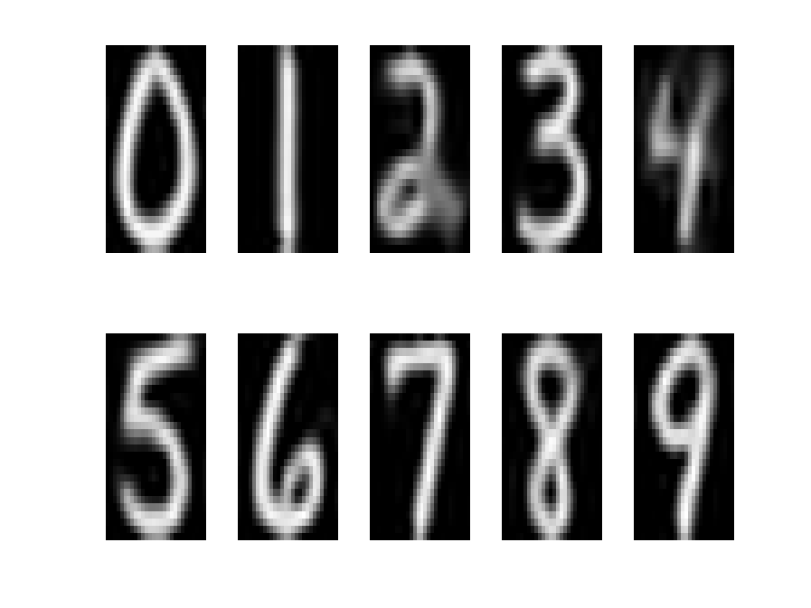
We show here the results of the statistical learning algorithm for this model. Figure 4 shows two runs of the algorithm for a non-noisy database with 1010 and 2020 images per class. Ten images per class are enough to obtain satisfactory template images with high contrast.

Although it was proved in [2] that the Kullback-Leibler divergence between q⁡(⋅,θ~)q(\cdot;\tilde{\theta}) and the common density function for observations from a given class converges to its minimal value on the family q⁡(⋅,θ)q(\cdot;\theta), we note that increasing the number of training images does not significantly improve the estimated photometric template. This apparently surprising fact can be explained as follows : since strong variations in appearance among the images may happened within a given class (think about topological changes for instance), the image distribution can not be perfectly represented as a distribution around a single template. This distribution is better represented as clustered around a major template and minor ones in a multimodal way. When the sample size is moderate, with a high probability, the sample contains basically images around the major mode and parametric model fits these data quite accurately. When the sample size increases, the minor modes start to play a significant role as “outliers” with respect to the major mode in the data, resulting in a slightly more blurry template trying to accommodate the different modes. One way to overcome this fact is to use some clustering methods as proposed in [2]. To visualize robustness with respect to the training set, we ran this algorithm with 2020 images per class randomly chosen in the whole database. The different runs are presented in Figure 5. The two left images show some templates which look like the ones obtained in the left image of Figure 4 with the 2020 first examples of the database. When outliers appear among the 2020 randomly chosen training images the template may become somewhat more blurry. This is observed for digits ’2’ and ’4’ (apparently the most variable digits) in the right image of Figure 5. For digits where the outliers are less far from the other images, the templates are stable.

Refer to caption
Refer to caption
Refer to caption
Fig. 5: Templates estimated with randomly chosen samples from the whole USPostal database. Each image is one run of the algorithm with same initial conditions but different training sets of 2020 images per digit each. The variability of the results is related to the huge variability inside the USPS database.
Refer to caption
Refer to caption
Refer to caption
Refer to caption
Fig. 6: Evolution of the templates with the algorithm iterations. Top line. Left: Mean gray level images of the 2020 training samples. Middle: template at the 50th iteration. Right: template at the 100th iteration. Bottom line: template at the 150th iteration. The improvement is visible , very fast for some very simple shapes as digit 11 and longer for very variable ones as digit 22. The higher geometric variability increases the fitting time of the algorithm.

The evolution of the template with the iterations can be viewed in Figure 6. The initialization of the template is the mean of the gray level images. As the iterations proceed, the templates become sharper. In particular, the estimated templates for digits with small geometrical variability converge very fast. For digits like ’2’ or ’4’, where the geometrical variability is higher, the convergence of the coupled parameters (photometry and geometry) is slowed down.

5.2 Photometric noise variance

Refer to caption
Fig. 7: Evolution of the estimated noise variance using 2020 images per class along the SAEM-MCMC algorithm. This confirms the visual effects seen on the templates : rapid convergence for some really constrained digits and slower convergence for very variable ones.

The evolution of the noise variance all along the SAEM-MCMC iterations is the same as the one observed with the “mode approximation EM” described in [2]. During the first iterations, the noise variance balances the inaccuracy of the estimated template which is simply the gray-level mean of the training set. As the iterations proceed, the template estimates become sharper as does the estimate of the covariance matrix for the geometry. This yields very small residual noise. Note that here the final noise variance, which is less than 0.10.1, for the SAEM-MCMC algorithm for all digits is less than the noise variance , which is between 0.20.2 and 0.30.3, for the mode approximation EM experimented in [2] in the one component run. This can be explained by the stochastic nature of the algorithm which enables it to escape from local minima provoking early terminations in the deterministic version.

5.3 Estimated geometric distribution

As mentioned previously we have to fix the value of the hyper-parameter aga_{g} of the prior on Γg\Gamma_{g}. This quantity plays a significant role in the results. Indeed, to satisfy the theoretical conditions we have to choose aga_{g} larger than 4​kg+14k_{g}+1 say 4×36+14\times 36+1 in our examples. From the geometry update equation, a barycenter between the ‘sample’ covariance and the prior, with the number nn of images and aga_{g} as coefficients, we find that the prior dominates when the training set is small. The covariance matrix stays close to the prior. Thus we need to decrease aga_{g} and find the best trade-off between the degenerate inverse Wishart and the weight of the prior in the covariance estimation. We fix this value with a visual criterion: both the templates and the generated sample with the learnt geometry have to be satisfactory. This yields ag=0.5a_{g}=0.5 or 0.10.1.

As we have observed from Figure 9, parameter estimation is robust regardless of whether the prior is degenerate or not. In addition, considering the update formulas, even if this law does not have a total weight equal to 11 it does not affect parameter estimation.

Refer to caption
Fig. 8: Effect of the prior distribution on the deformation : 20 synthetic examples per class generated with the estimated template but the prior covariance matrix (inverse video).
Refer to caption
Fig. 9: Effect of the estimated geometric distribution : 40 synthetic examples per class generated with the estimated parameters: 20 with the direct deformations and 20 with the symmetric deformations (inverse video).

In Figure 9, we show a sample of some synthetic digits modeled by deformation templates drawn with the estimated parameters. Note that the resulting digits in Figure 9 look like some elements of the training set and seem to explain these data correctly, whereas the prior produces some non-relevant local deformations (cf. Figure (8)). In particular, for some especially geometrically constrained digits such as 00 or 11, the geometry variability reflects their constraints. For digits like the 22s, the training set is heterogeneous and shows a large geometrical variability. When comparing to the deformations obtained by the mode approximation to EM in [2], it seems that here we obtain a more variable geometry. This might be because with a stochastic algorithm, we explore the posterior density and do not only concentrate at its mode. This allows some more exotic deformations corresponding to realizations of the missing variable 𝜷\boldsymbol{\beta} which may belong to the tail of the law. Another reason may be that for such digits, the mode approximation gets stuck in a local minimum of the matching energy. Jumping out of this configuration would require a large deformation (not allowed by the gradient descent since it would increase the energy again). However, such a deformation can be proposed leading to acceptance by the stochastic algorithm. Subsequently the deformed template may better fit the observations, leading to acceptance of these large deformations. This also leads to a lower value of the residual noise and may also explain the low noise variance estimated by the stochastic EM algorithm.

5.4 Noise effect


Fig. 10: Two images examples per class of the noisy training set (variance: top: σ2=1\sigma^{2}=1, bottom: σ2=2\sigma^{2}=2).


Fig. 11: Estimated prototypes in a noisy setting σ2=1\sigma^{2}=1: Left: with the mode approximation algorithm. Right: with the SAEM-MCMC coupling procedure.


Fig. 12: Estimated prototypes in a noisy setting σ2=2\sigma^{2}=2: Left: with the mode approximation algorithm. Right: with the SAEM-MCMC coupling procedure.

As shown in [2], in the presence of noise, the mode approximation algorithm does not converge towards the MAP estimator. In our setting, the consistency of the “SAEM like” algorithm has been proved independently of the training set, and thus noisy images can also be treated exactly the same way. These are the results we present here. Figure 10 shows two training examples per class for noise variance values σ2=1\sigma^{2}=1 and σ2=2\sigma^{2}=2. In Figures 11 and 12, we show the estimated templates for the noisy training set containing 20 images for both methods. Even if the mode approximation algorithm does not diverge, it cannot fit the template for digits with a high variability. In contrast, the stochastic EM gives acceptable contrasted templates which look like those obtained in Figure 4. This becomes more significant as we increase the variance of the additive noise we introduce in the training set.

Concerning the choice of the hyper-parameters, it is not necessary to change all of them. For the photometric variance of the spline kernel, a small one could create some non-smooth templates and a large kernel would smooth the noise effect. However, we can keep the geometric hyper-parameters unchanged. We are presenting here only experiments which seemed to provide a reasonable tradeoff between these effects.

Refer to caption
Fig. 13: Effect of the noise on the geometric parameter estimation : 40 synthetic examples per class generated with the parameters estimated from the noisy training set (additive noise variance of 11, inverse video).

The geometry is also well estimated despite the high level of noise in the training set. Figure 13 shows some synthetic examples, in which parameters are learnt from the training set with an additive noise variance of one. The two lines correspond to deformations and their symmetric deformation. This sample looks like the synthetic samples learnt on non-noisy images even if some examples are not relevant. However, the global behavior has been learnt.

The algorithm manages to catch the photometry (a contrasted and smoothed template), the geometry of the shapes and to “separate” the additive noise.

The number of iterations needed to reach the convergence point in the noisy setting is about twice that of the non-noisy case. The template takes the longest time to converge and the estimate of σ2\sigma^{2} converges in a few iterations. In particular, the templates obtained in the left panel of Figure 4 with only 1010 images per training digit set are obtained with a heating period of 2525 iterations and 55 more steps with memory. The templates of Figure 11, right picture, require 100100 to 125125 heating iterations in the 150150 global iterations. This is understandable since the algorithm has to cope with variations due to the noise and thus needs a longer time to fit the model.

6 Proof of Theorem 4

Here we demonstrate Theorem 4, i.e. the stochastic approximation sequence satisfies assumptions (A1’) (ii), (iii), (iv), (A2) and (A3’).

We recall that in this section, the parameter σ2\sigma^{2} is fixed so that θ=(α,Γ)\theta=(\alpha,\Gamma). The sufficient statistic vector SS, the set 𝒮\mathcal{S} as well as the explicit expression of θ^​(s)\hat{\theta}(s) have been given in Subsection 4.2. As noted, θ^\hat{\theta} is a smooth function of 𝒮\mathcal{S}.

We will prove that these conditions hold for any p≥1p\geq 1 and a∈]0,1[a\in]0,1[.

6.1 Proof of assumption (A1’)

We recall the functions H,hH,\ h and w\ w as in [8] defined as follows:

Hs​(𝜷)\displaystyle H_{s}(\boldsymbol{\beta}) =\displaystyle= S⁡(𝜷)−s,\displaystyle S(\boldsymbol{\beta})-s\,,
h⁡(s)\displaystyle h(s) =\displaystyle= ∫ℝNHs​(𝜷)​qp​o​s​t​(𝜷|𝕪,θ^​(s))​𝑑𝜷,\displaystyle\int_{\mathbb{R}^{N}}H_{s}(\boldsymbol{\beta})q_{post}(\boldsymbol{\beta}|\mathbb{y},\hat{\theta}(s))d\boldsymbol{\beta}\,,
w⁡(s)\displaystyle w(s) =\displaystyle= −l​(θ^​(s)).\displaystyle-l(\hat{\theta}(s))\,.

As shown in [8], with these functions, we satisfy (A1’(iii)) and (A1’(iv)).

Moreover, since the interpolation kernel KpK_{p} is bounded, there exist A>0A>0 and B∈Symkp+B\in\text{Sym}_{k_{p}}^{+} such that for any 𝜷∈ℝN\boldsymbol{\beta}\in\mathbb{R}^{N}, we have

‖S1​(𝜷)‖≤A, 0≤S2​(𝜷)≤B​ and ​0≤S3​(𝜷),\|S_{1}(\boldsymbol{\beta})\|\leq A,\ 0\leq S_{2}(\boldsymbol{\beta})\leq B\text{ and }0\leq S_{3}(\boldsymbol{\beta})\,,

where, for any symmetric matrices BB and B′B^{\prime}, we say that B≤B′B\leq B^{\prime} if B′−BB^{\prime}-B is a non-negative symmetric matrix.

We define the set 𝒮a\mathcal{S}_{a} by

𝒮a≜{S∈𝒮|∥S1∥≤A, 0≤S2≤B and 0≤S3}.\mathcal{S}_{a}\triangleq\{\ S\in\mathcal{S}\ |\ \|S_{1}\|\leq A,\ 0\leq S_{2}\leq B\ \text{ and }0\leq S_{3}\ \}\,.

Since the constraints are obviously convex and closed, we get that 𝒮a\mathcal{S}_{a} is a closed convex subset of ℝns\mathbb{R}^{n_{s}} such that

𝒮a⊂𝒮⊂ℝns\mathcal{S}_{a}\subset\mathcal{S}\subset\mathbb{R}^{n_{s}}

and satisfying

s+ρHs(𝜷)∈𝒮a for any ρ∈[0,1] any s∈𝒮a and any 𝜷∈ℝN.s+\rho H_{s}(\boldsymbol{\beta})\in\mathcal{S}_{a}\ \text{ for any $\rho\in[0,1]$ any $s\in\mathcal{S}_{a}$ and any $\boldsymbol{\beta}\in\mathbb{R}^{N}$.}

We now focus on the first two points. As ll and θ^\hat{\theta} are continuous functions, we only need to prove that 𝒲M∩𝒮a\mathcal{W}_{M}\cap\mathcal{S}_{a} is a bounded set for a constant M∈ℝ+∗M\in\mathbb{R}^{*}_{+} with:

𝒲M={s∈𝒮,w⁡(s)≤M}.\mathcal{W}_{M}=\{s\in\mathcal{S},\ w(s)\leq M\}\,.

On 𝒮a\mathcal{S}_{a}, s1s_{1} and s2s_{2} are bounded; writing θ^​(s)=(α⁡(s),Γ⁡(s))\hat{\theta}(s)=(\alpha(s),\Gamma(s)), we deduce from (3) and from the boundedness of KpK_{p} that α⁡(s)\alpha(s) is bounded on 𝒮a\mathcal{S}_{a} and |yi−Kpβi​α​(s)||y_{i}-K_{p}^{\beta_{i}}\alpha(s)| is uniformly bounded on βi∈ℝ2​kg\beta_{i}\in\mathbb{R}^{2k_{g}} and s∈𝒮as\in\mathcal{S}_{a}. Hence (recall that σ2\sigma^{2} is fixed here), there exists an η>0\eta>0 such that qc​(𝕪|𝜷,θ^​(s))≥ηq_{c}(\mathbb{y}|\boldsymbol{\beta},\hat{\theta}(s))\geq\eta for any s∈𝒮as\in\mathcal{S}_{a} and 𝜷∈ℝN\boldsymbol{\beta}\in\mathbb{R}^{N}. Thus,

w(s)≥−log(∫qm(𝜷,θ^(s))d𝜷)+C≥−log(qp​a​r​a(θ^(s)))+C≥−log(qp​a​r​a|Γ(Γ(s)))+C,w(s)\geq-\log\left(\int q_{m}(\boldsymbol{\beta},\hat{\theta}(s))d\boldsymbol{\beta}\right)+\text{C}\geq-\log(q_{para}(\hat{\theta}(s)))+\text{C}\geq-\log({q_{para}}_{|_{\Gamma}}(\Gamma(s)))+\text{C}\,,

where C is a constant independent of s∈Sas\in S_{a}. Since

−log(qp​a​r​a|Γ(Γg))=ag2(⟨Γg−1,Σg⟩F+log|Γg|)≥ag2log|Γg|-\log({q_{para}}_{|_{\Gamma}}(\Gamma_{g}))=\frac{a_{g}}{2}\left(\langle\Gamma_{g}^{-1},\Sigma_{g}\rangle_{F}+\log|\Gamma_{g}|\right)\geq\frac{a_{g}}{2}\log|\Gamma_{g}|

and

lim‖s‖→+∞,s∈𝒮alog⁡(|Γg​(s)|)=lim‖s‖→+∞,s∈𝒮alog⁡(|(s3+ag​Σg)/(n+ag)|)=+∞,\lim_{\|s\|\to+\infty,s\in\mathcal{S}_{a}}\log(|\Gamma_{g}(s)|)=\lim_{\|s\|\to+\infty,s\in\mathcal{S}_{a}}\log(|(s_{3}+a_{g}\Sigma_{g})/(n+a_{g})|)=+\infty,

we deduce that

lim‖s‖→+∞,s∈𝒮aw⁡(s)=+∞.\lim_{\|s\|\to+\infty,s\in\mathcal{S}_{a}}w(s)=+\infty\,.

Since ww is continuous and 𝒮a\mathcal{S}_{a} is closed, this proves (A1’(ii)).

6.2 Proof of assumption (A2)

We prove a classical sufficient condition (DRI1), used in [6] which will imply (A2) under the condition that HsH_{s} is dominated by VV for any s∈𝒦s\in\mathcal{K}.

(DRI1)

For any s∈𝒮s\in\mathcal{S}, 𝚷θ^​(s)\boldsymbol{\Pi}_{\hat{\theta}(s)} is ϕ−\phi-irreducible and aperiodic. In addition there exist a function V:ℝN→[1,∞[V:\mathbb{R}^{N}\to[1,\infty[ and p≥2p\geq 2 such that for any compact subset 𝒦⊂𝒮\mathcal{K}\subset\mathcal{S}, there exist an integer mm and constants 0<λ<10<\lambda<1, B>0B>0, κ>0\kappa>0, δ>0\delta>0, a subset C of ℝN\mathbb{R}^{N} and a probability measure ν\nu such that

sups∈𝒦𝚷θ^​(s)m​Vp​(𝜷)\displaystyle\sup\limits_{s\in\mathcal{K}}\boldsymbol{\Pi}_{\hat{\theta}(s)}^{m}V^{p}(\boldsymbol{\beta}) ≤\displaystyle\leq λ​Vp​(𝜷)+B​𝟙C​(𝜷),\displaystyle\lambda V^{p}(\boldsymbol{\beta})+B\mathds{1}_{\texttt{C}}(\boldsymbol{\beta})\,, (23)
sups∈𝒦𝚷θ^​(s)​Vp​(𝜷)\displaystyle\sup\limits_{s\in\mathcal{K}}\boldsymbol{\Pi}_{\hat{\theta}(s)}V^{p}(\boldsymbol{\beta}) ≤\displaystyle\leq κ​Vp​(𝜷)∀𝜷∈ℝN,\displaystyle\kappa V^{p}(\boldsymbol{\beta})\ \ \forall\boldsymbol{\beta}\in\mathbb{R}^{N}\,, (24)
infs∈𝒦𝚷θ^​(s)m​(𝜷,A)\displaystyle\inf\limits_{s\in\mathcal{K}}\boldsymbol{\Pi}_{\hat{\theta}(s)}^{m}(\boldsymbol{\beta},A) ≥\displaystyle\geq δ​ν​(A)∀𝜷∈C,∀A∈ℬ⁡(ℝN).\displaystyle\delta\nu(A)\ \ \forall\boldsymbol{\beta}\in\texttt{C},\forall A\in\mathcal{B}(\mathbb{R}^{N})\,. (25)
Remark 5.

Note that condition (25) is equivalent to the existence of a small set C (defined below) which only depends on 𝒦\mathcal{K}.

Notation 1.

Let (ej)1≤j≤N(e_{j})_{1\leq j\leq N} be the canonical basis of ℝN\mathbb{R}^{N}. For any 1≤j≤N1\leq j\leq N, let Eθ,j≜{𝛃∈ℝN|⟨𝛃,ej⟩θ=0}E_{\theta,j}\triangleq\{\ \boldsymbol{\beta}\in\mathbb{R}^{N}\ |\ \langle\boldsymbol{\beta},e_{j}\rangle_{\theta}=0\} be the orthogonal space of Span​{ej}\text{Span}\{e_{j}\} and pθ,jp_{\theta,j} be the orthogonal projection on Eθ,jE_{\theta,j} i.e.

pθ,j​(𝜷)≜𝜷−⟨𝜷,ej⟩θ‖ej‖θ2​ej,p_{\theta,j}(\boldsymbol{\beta})\triangleq\boldsymbol{\beta}-\frac{\langle\boldsymbol{\beta},e_{j}\rangle_{\theta}}{\|e_{j}\|^{2}_{\theta}}e_{j}\,,

where ⟨𝛃,𝛃′⟩θ=∑i=1nβit​Γg−1​βi′\langle\boldsymbol{\beta},\boldsymbol{\beta}^{\prime}\rangle_{\theta}=\sum_{i=1}^{n}\beta_{i}^{t}\Gamma_{g}^{-1}\beta^{\prime}_{i} for θ=(α,Γg)\theta=(\alpha,\Gamma_{g}) (i.e. the natural dot product associated with the covariance matrix Γg\Gamma_{g}) and ∥.∥θ\|.\|_{\theta} the corresponding norm.

We denote for any 1≤j≤N1\leq j\leq N and θ∈Θ\theta\in\Theta by 𝚷θ,j\boldsymbol{\Pi}_{\theta,j} the Markov kernel on ℝN\mathbb{R}^{N} (5) associated with the Metropolis-Hastings step of the jj-th Gibbs sampler step on 𝛃\boldsymbol{\beta}. We have 𝚷θ=𝚷θ,N∘⋯∘𝚷θ,1\boldsymbol{\Pi}_{\theta}=\boldsymbol{\Pi}_{\theta,N}\circ\cdots\circ\boldsymbol{\Pi}_{\theta,1}.

We first recall the definition of a small set:

Definition 1.

(cf. [15]) A set ℰ∈ℬ⁡(𝒳)\mathcal{E}\in\mathcal{B}(\mathcal{X}) is called a small set for the kernel 𝚷\boldsymbol{\Pi} if there exist an m>0m>0, and a non trivial measure νm\nu_{m} on ℬ⁡(𝒳)\mathcal{B}(\mathcal{X}), such that for all 𝛃∈ℰ\boldsymbol{\beta}\in\mathcal{E}, B∈ℬ⁡(𝒳)B\in\mathcal{B}(\mathcal{X}),

𝚷m​(𝜷,B)≥νm​(B).\boldsymbol{\Pi}^{m}(\boldsymbol{\beta},B)\geq\nu_{m}(B). (26)

When (26) holds, we say that ℰ\mathcal{E} is νm\nu_{m}-small.

We now prove the following lemma which give the existence of the small set C in (DRI1):

Lemma 5.

Let ℰ\mathcal{E} be a compact subset of ℝN\mathbb{R}^{N} and 𝒦\mathcal{K} a compact subset of 𝒮\mathcal{S}. Then ℰ\mathcal{E} is a small set of ℝN\mathbb{R}^{N} for 𝚷θ^​(s)\boldsymbol{\Pi}_{\hat{\theta}(s)} for any s∈𝒦s\in\mathcal{K}.

Proof.

First note that there exists an ac>0a_{c}>0 such that for any θ∈Θ\theta\in\Theta, any 𝜷∈ℝN\boldsymbol{\beta}\in\mathbb{R}^{N} and any b∈ℝb\in\mathbb{R}, the acceptance rate rj​(𝜷j,b,𝜷−j,θ)r_{j}(\boldsymbol{\beta}^{j},b;\boldsymbol{\beta}^{-j},\theta) is uniformly bounded below by aca_{c} so that for any 1≤j≤N1\leq j\leq N and any non-negative function ff,

𝚷θ,j​f​(𝜷)≥ac​∫ℝf⁡(𝜷−j+b​ej)​qj​(b|𝜷−j,θ)​𝑑b=ac​∫ℝf⁡(pθ,j​(𝜷)+z​ej/‖ej‖θ)​g0,1​(z)​𝑑z,\boldsymbol{\Pi}_{\theta,j}f(\boldsymbol{\beta})\geq a_{c}\int_{\mathbb{R}}f(\boldsymbol{\beta}^{-j}+be_{j})q_{j}(b|\boldsymbol{\beta}^{-j},\theta)db=a_{c}\int_{\mathbb{R}}f(p_{\theta,j}(\boldsymbol{\beta})+ze_{j}/\|e_{j}\|_{\theta})g_{0,1}(z)dz\,,

where g0,1g_{0,1} is the density of the standard Gaussian distribution 𝒩⁡(0,1)\mathcal{N}(0,1).

By induction, we have

𝚷θ​f​(𝜷)≥acN​∫ℝNf⁡(pθ,N,1​(𝜷)+∑j=1Nzj​pθ,N,j+1​(ej)/‖ej‖θ)​∏j=1Ng0,1​(zj)​d​zj,\boldsymbol{\Pi}_{\theta}f(\boldsymbol{\beta})\geq a_{c}^{N}\int_{\mathbb{R}^{N}}f\left(p_{\theta,N,1}(\boldsymbol{\beta})+\sum_{j=1}^{N}z_{j}p_{\theta,N,j+1}(e_{j})/\|e_{j}\|_{\theta}\right)\prod_{j=1}^{N}g_{0,1}(z_{j})dz_{j}\,, (27)

where pθ,q,r=pθ,r∘pθ,r−1∘⋯∘pθ,qp_{\theta,q,r}=p_{\theta,r}\circ p_{\theta,r-1}\circ\cdots\circ p_{\theta,q} for any integers q≤rq\leq r and pθ,N,N+1=Idp_{\theta,N,N+1}=\text{Id}.

Let Aθ∈ℒ⁡(ℝN)A_{\theta}\in\mathcal{L}(\mathbb{R}^{N}) be the linear mapping on ℝN\mathbb{R}^{N} defined by

Aθ​z=∑j=1Nzj​pθ,N,j+1​(ej)/‖ej‖θ.A_{\theta}z=\sum_{j=1}^{N}z_{j}p_{\theta,N,j+1}(e_{j})/\|e_{j}\|_{\theta}\,.

One easily checks that for any 1≤k≤N1\leq k\leq N, Span{pθ,N,j+1(ej),k≤j≤N}=Span{ej|k≤j≤N}\text{Span}\{\ p_{\theta,N,j+1}(e_{j}),\ k\leq j\leq N\}=\text{Span}\{e_{j}\ |\ k\leq j\leq N\} so that AθA_{\theta} is an invertible mapping. By a change of variable, we get

∫ℝNf⁡(pθ,N,1​(𝜷)+Aθ​z1N)​∏j=1Ng0,1​(zj)​d​zj=∫ℝNf⁡(u)​gpθ,N,1​(𝜷),Aθ​Aθt​(u)​𝑑u,\int_{\mathbb{R}^{N}}f\left(p_{\theta,N,1}(\boldsymbol{\beta})+A_{\theta}z_{1}^{N}\right)\prod_{j=1}^{N}g_{0,1}(z_{j})dz_{j}=\int_{\mathbb{R}^{N}}f(u)g_{p_{\theta,N,1}(\boldsymbol{\beta}),A_{\theta}A_{\theta}^{t}}(u)du\,,

where gμ,Σg_{\mu,\Sigma} stands for the density of the normal law 𝒩⁡(μ,Σ)\mathcal{N}(\mu,\Sigma). Since θ→Aθ\theta\to A_{\theta} is smooth on the set of invertible mappings in θ\theta, we deduce that there exist two constants c𝒦>0c_{\mathcal{K}}>0 and C𝒦>0C_{\mathcal{K}}>0 such that c𝒦​Id≤Aθ​Aθt≤Id/c𝒦c_{\mathcal{K}}\text{Id}\leq A_{\theta}A_{\theta}^{t}\leq\text{Id}/c_{\mathcal{K}} and gpθ,N,1​(𝜷),Aθ​Aθt​(u)≥C𝒦​gpθ,N,1​(𝜷),Id/c𝒦​(u)g_{p_{\theta,N,1}(\boldsymbol{\beta}),A_{\theta}A_{\theta}^{t}}(u)\geq C_{\mathcal{K}}g_{p_{\theta,N,1}(\boldsymbol{\beta}),\text{Id}/c_{\mathcal{K}}}(u) uniformly for θ=θ^​(s)\theta=\hat{\theta}(s) with s∈𝒦s\in\mathcal{K}. Assuming that 𝜷∈ℰ\boldsymbol{\beta}\in\mathcal{E}, since θ→pθ,N,1\theta\to p_{\theta,N,1} is smooth and ℰ\mathcal{E} is compact, we have sup𝜷∈ℰ,θ=θ^​(s),s∈𝒦‖pθ,N,1​(𝜷)‖<∞\sup\limits_{\boldsymbol{\beta}\in\mathcal{E},\theta=\hat{\theta}(s),\ s\in\mathcal{K}}\|p_{\theta,N,1}(\boldsymbol{\beta})\|<\infty. Therefore, there exist C𝒦′>0C_{\mathcal{K}}^{\prime}>0 and c𝒦′>0c_{\mathcal{K}}^{\prime}>0 such that for any (u,𝜷)∈ℝN×ℰ(u,\boldsymbol{\beta})\in\mathbb{R}^{N}\times\mathcal{E} and any θ=θ^​(s),s∈𝒦\theta=\hat{\theta}(s),\ s\in\mathcal{K}

gpθ,N,1​(𝜷),Aθ​Aθt​(u)≥C𝒦′​g0,Id/c𝒦′​(u).g_{p_{\theta,N,1}(\boldsymbol{\beta}),A_{\theta}A_{\theta}^{t}}(u)\geq C_{\mathcal{K}}^{\prime}g_{0,\text{Id}/c_{\mathcal{K}}^{\prime}}(u)\,.\\ (28)

Using (27) and (28), we deduce that for any AA, for any s∈𝒦s\in\mathcal{K} and θ=θ^​(s)\theta=\hat{\theta}(s),

𝚷θ​(𝜷,A)≥C𝒦′​acN​ν𝒦​(A),\boldsymbol{\Pi}_{\theta}(\boldsymbol{\beta},A)\geq C_{\mathcal{K}}^{\prime}a_{c}^{N}\nu_{\mathcal{K}}(A)\,,

with ν𝒦\nu_{\mathcal{K}} equals to the density of the normal law 𝒩⁡(0,Id/c𝒦′)\mathcal{N}(0,\text{Id}/c_{\mathcal{K}}^{\prime}).

This yields the existence of the small set as well as equation (25). ∎

This property also implies the ϕ\phi-irreducibility of the Markov chain (𝜷k)k(\boldsymbol{\beta}_{k})_{k} and its aperiodicity (cf. [15] p121).

We set V:ℝN→[1,+∞[V:\mathbb{R}^{N}\to[1,+\infty[ as the following function

V⁡(𝜷)=1+‖𝜷‖2.V(\boldsymbol{\beta})=1+\|\boldsymbol{\beta}\|^{2}\,. (29)

We, in fact, have the following property : ∃C𝒦>0\exists\ C_{\mathcal{K}}>0 such that : ∀𝜷∈ℝN\forall\boldsymbol{\beta}\in\mathbb{R}^{N},

sups∈𝒦‖Hs​(𝜷)‖≤C𝒦​V​(𝜷).\sup\limits_{s\in\mathcal{K}}\|H_{s}(\boldsymbol{\beta})\|\leq C_{\mathcal{K}}\ V(\boldsymbol{\beta})\,.

This condition is required for the implication of (A2) by (DRI1).

We now prove condition (24).

Let 𝒦\mathcal{K} be a compact subset of 𝒮\mathcal{S} and p≥1p\geq 1. For any 1≤j≤N1\leq j\leq N, any s∈𝒦s\in\mathcal{K} and θ=θ^​(s)\theta=\hat{\theta}(s), we have

𝚷θ,j​Vp​(𝜷)≤Vp​(𝜷)+∫ℝVp​(pθ,j​(𝜷)+z​ej/‖ej‖θ)​g0,1​(z)​𝑑z.\boldsymbol{\Pi}_{\theta,j}V^{p}(\boldsymbol{\beta})\leq V^{p}(\boldsymbol{\beta})+\int_{\mathbb{R}}V^{p}(p_{\theta,j}(\boldsymbol{\beta})+ze_{j}/\|e_{j}\|_{\theta})g_{0,1}(z)dz\,.

Since V⁡(𝜷+h)≤2​(V⁡(𝜷)+V⁡(h))V(\boldsymbol{\beta}+h)\leq 2(V(\boldsymbol{\beta})+V(h)) for any 𝜷,h∈ℝN\boldsymbol{\beta},h\in\mathbb{R}^{N} and since there exist two constants c𝒦>0c_{\mathcal{K}}>0 and C𝒦>0C_{\mathcal{K}}>0 such that for any 𝜷∈ℝN\boldsymbol{\beta}\in\mathbb{R}^{N}, θ∈θ^​(𝒦)\theta\in\hat{\theta}(\mathcal{K}), ‖pθ,j​(𝜷)‖≤C𝒦​‖𝜷‖\|p_{\theta,j}(\boldsymbol{\beta})\|\leq C_{\mathcal{K}}\|\boldsymbol{\beta}\| and ‖ej‖θ≥1/c𝒦\|e_{j}\|_{\theta}\geq 1/c_{\mathcal{K}}, we have

∫ℝVp​(pθ,j​(𝜷)+z​ej/‖ej‖θ)​g0,1​(z)​𝑑z≤2p​C𝒦p​Vp​(𝜷)​∫ℝ(1+V⁡(c𝒦​z​ej))p​g0,1​(z)​𝑑z.\int_{\mathbb{R}}V^{p}(p_{\theta,j}(\boldsymbol{\beta})+ze_{j}/\|e_{j}\|_{\theta})g_{0,1}(z)dz\leq 2^{p}C_{\mathcal{K}}^{p}V^{p}(\boldsymbol{\beta})\int_{\mathbb{R}}(1+V(c_{\mathcal{K}}ze_{j}))^{p}g_{0,1}(z)dz\,.

We deduce that there exists an C𝒦′>0C_{\mathcal{K}}^{\prime}>0 such that for any 𝜷∈ℝN\boldsymbol{\beta}\in\mathbb{R}^{N}

supθ=θ^​(s),s∈𝒦𝚷θ,j​Vp​(𝜷)≤C𝒦′​Vp​(𝜷).\sup_{\theta=\hat{\theta}(s),s\in\mathcal{K}}\boldsymbol{\Pi}_{\theta,j}V^{p}(\boldsymbol{\beta})\leq C_{\mathcal{K}}^{\prime}V^{p}(\boldsymbol{\beta})\,.

Then, by composition 𝚷θ​Vp​(𝜷)≤C𝒦′N​Vp​(𝜷)\boldsymbol{\Pi}_{\theta}V^{p}(\boldsymbol{\beta})\leq C_{\mathcal{K}}^{\prime N}V^{p}(\boldsymbol{\beta}) and (24) holds for any p≥1p\geq 1.

Now consider the Drift condition (23).

To prove this inequality, we prove the same inequality for a subsidiary function VθV_{\theta} which depends on the parameters θ\theta and then we deduce the result for VV.
So let us define for any θ=(α,Γg)\theta=(\alpha,\Gamma_{g}) the function Vθ​(𝜷)≜1+‖𝜷‖θ2V_{\theta}(\boldsymbol{\beta})\triangleq 1+\|\boldsymbol{\beta}\|_{\theta}^{2}.

Lemma 6.

Let KK be a compact subset of Θ\Theta. For any p≥1p\geq 1, there exist an 0≤ρK<10\leq\rho_{K}<1 and an CK>0C_{K}>0 such that for any θ∈K\theta\in K, any 𝛃∈ℝN\boldsymbol{\beta}\in\mathbb{R}^{N} we have

𝚷θ​Vθp​(𝜷)≤ρK​Vθp​(𝜷)+CK.\boldsymbol{\Pi}_{\theta}V_{\theta}^{p}(\boldsymbol{\beta})\leq\rho_{K}V_{\theta}^{p}(\boldsymbol{\beta})+C_{K}\,.
Proof.

The proposal distribution for 𝚷θ,j\boldsymbol{\Pi}_{\theta,j} is given by q⁡(𝜷|𝜷−j,y,θ)=lawpθ,j​(𝜷)+z​ej‖ej‖θq(\boldsymbol{\beta}\ |\ \boldsymbol{\beta}^{-j},y,\theta)\stackrel{{\scriptstyle\text{law}}}{{=}}p_{\theta,j}(\boldsymbol{\beta})+z\frac{e_{j}}{\|e_{j}\|_{\theta}} where z∼𝒩⁡(0,1)z\sim\mathcal{N}(0,1). Then, there exists CKC_{K} such that for any 𝜷∈ℝN\boldsymbol{\beta}\in\mathbb{R}^{N} and any measurable set A∈ℬ⁡(ℝN)A\in\mathcal{B}(\mathbb{R}^{N})

𝚷θ,j​(𝜷,A)=(1−aθ,𝜷)​𝟙A​(𝜷)+aθ,𝜷​∫ℝ𝟙A​(pθ,j​(𝜷)+z​ej‖ej‖θ)​g0,1​(z)​𝑑z,\boldsymbol{\Pi}_{\theta,j}(\boldsymbol{\beta},A)=(1-a_{\theta,\boldsymbol{\beta}})\mathds{1}_{A}(\boldsymbol{\beta})+a_{\theta,\boldsymbol{\beta}}\int_{\mathbb{R}}\mathds{1}_{A}\left(p_{\theta,j}(\boldsymbol{\beta})+z\frac{e_{j}}{\|e_{j}\|_{\theta}}\right)g_{0,1}(z)dz\,,

where aθ,𝜷≥aca_{\theta,\boldsymbol{\beta}}\geq a_{c} (aca_{c} is a lower bound for the acceptance rate),

Since ⟨pθ,j​(𝜷),ej⟩θ=0\langle p_{\theta,j}(\boldsymbol{\beta}),e_{j}\rangle_{\theta}=0, we get Vθ​(pθ,j​(𝜷)+z​ej‖ej‖θ)=Vθ​(pθ,j​(𝜷))+z2V_{\theta}\left(p_{\theta,j}(\boldsymbol{\beta})+z\frac{e_{j}}{\|e_{j}\|_{\theta}}\right)=V_{\theta}(p_{\theta,j}(\boldsymbol{\beta}))+z^{2} and

𝚷θ,j​Vθp​(𝜷)=(1−aθ,𝜷)​Vθp​(𝜷)+aθ,𝜷​∫ℝ(Vθ​(pθ,j​(𝜷))+z2)p​g0,1​(z)​𝑑z≤(1−aθ,𝜷)​Vθp​(𝜷)+aθ,𝜷​(Vθp​(pθ,j​(𝜷))+CK​Vθp−1​(pθ,j​(𝜷))​∫ℝ(1+z2)p​g0,1​(z)​dz)≤(1−aθ,𝜷)​Vθp​(𝜷)+aθ,𝜷​Vθp​(pθ,j​(𝜷))+CK′​Vθp−1​(pθ,j​(𝜷)).\boldsymbol{\Pi}_{\theta,j}V_{\theta}^{p}(\boldsymbol{\beta})=(1-a_{\theta,\boldsymbol{\beta}})V^{p}_{\theta}(\boldsymbol{\beta})+a_{\theta,\boldsymbol{\beta}}\int_{\mathbb{R}}\left(V_{\theta}(p_{\theta,j}(\boldsymbol{\beta}))+z^{2}\right)^{p}g_{0,1}(z)dz\\ \leq(1-a_{\theta,\boldsymbol{\beta}})V^{p}_{\theta}(\boldsymbol{\beta})+a_{\theta,\boldsymbol{\beta}}\left(V^{p}_{\theta}(p_{\theta,j}(\boldsymbol{\beta}))+C_{K}V^{p-1}_{\theta}(p_{\theta,j}(\boldsymbol{\beta}))\int_{\mathbb{R}}(1+z^{2})^{p}g_{0,1}(z)dz\right)\\ \leq(1-a_{\theta,\boldsymbol{\beta}})V^{p}_{\theta}(\boldsymbol{\beta})+a_{\theta,\boldsymbol{\beta}}V^{p}_{\theta}(p_{\theta,j}(\boldsymbol{\beta}))+C^{\prime}_{K}V^{p-1}_{\theta}(p_{\theta,j}(\boldsymbol{\beta}))\,.

We have used in the last inequality the fact that a Gaussian variable has bounded moments of any order. Since aθ,𝜷≥aca_{\theta,\boldsymbol{\beta}}\geq a_{c} and ‖pθ,j​(𝜷)‖θ≤‖𝜷‖θ\|p_{\theta,j}(\boldsymbol{\beta})\|_{\theta}\leq\|\boldsymbol{\beta}\|_{\theta} (pθ,jp_{\theta,j} is an orthonormal projection for the dot product ⟨⋅,⋅⟩θ\langle\cdot,\cdot\rangle_{\theta}), we get that ∀η>0\forall\,\eta>0, ∃CK,η\exists\,C_{K,\eta} such that ∀𝜷∈ℝN\forall\,\boldsymbol{\beta}\in\mathbb{R}^{N} and ∀θ∈K\forall\,\theta\in K

𝚷θ,j​Vθp​(𝜷)≤(1−ac)​Vθp​(𝜷)+(ac+η)​Vθp​(pθ,j​(𝜷))+CK,η.\boldsymbol{\Pi}_{\theta,j}V^{p}_{\theta}(\boldsymbol{\beta})\leq(1-a_{c})V^{p}_{\theta}(\boldsymbol{\beta})+(a_{c}+\eta)V_{\theta}^{p}(p_{\theta,j}(\boldsymbol{\beta}))+C_{K,\eta}\,.

By induction, we show that

𝚷θ​Vθp​(𝜷)≤∑u∈{0,1}N∏j=1N(1−ac)1−uj​(ac+η)uj​Vθp​(pθ,u​(𝜷))+CK,ηη​((1+η)N+1−1),\boldsymbol{\Pi}_{\theta}V^{p}_{\theta}(\boldsymbol{\beta})\leq\sum_{u\in\{0,1\}^{N}}\prod_{j=1}^{N}(1-a_{c})^{1-u_{j}}(a_{c}+\eta)^{u_{j}}V^{p}_{\theta}(p_{\theta,u}(\boldsymbol{\beta}))+\frac{C_{K,\eta}}{\eta}((1+\eta)^{N+1}-1)\,,

where pθ,u=((1−uN)Id+uNpθ,N)∘⋯∘((1−u1)Id+u1pθ,1)p_{\theta,u}=((1-u_{N})\text{Id}+u_{N}p_{\theta,N})\circ\cdots\circ((1-u_{1})\text{Id}+u_{1}p_{\theta,1}). Let pθ=pθ,N∘⋯∘pθ,1p_{\theta}=p_{\theta,N}\circ\cdots\circ p_{\theta,1} and note that pθ,jp_{\theta,j} is contracting so that

𝚷θ​Vθp​(𝜷)≤bc,η​Vθp​(𝜷)+(ac+η)N​Vθp​(pθ​(𝜷))+CK,ηη​((1+η)N+1),\boldsymbol{\Pi}_{\theta}V^{p}_{\theta}(\boldsymbol{\beta})\leq b_{c,\eta}V^{p}_{\theta}(\boldsymbol{\beta})+(a_{c}+\eta)^{N}V^{p}_{\theta}(p_{\theta}(\boldsymbol{\beta}))+\frac{C_{K,\eta}}{\eta}((1+\eta)^{N+1})\,,

for bc,η=(∑u∈{0,1}N,u≠𝟏∏j=1N(1−ac)1−uj​(ac+η)uj)b_{c,\eta}=\left(\sum_{u\in\{0,1\}^{N},\ u\neq\mathbf{1}}\prod_{j=1}^{N}(1-a_{c})^{1-u_{j}}(a_{c}+\eta)^{u_{j}}\right).

To end the proof, we need to check that pθp_{\theta} is strictly contracting uniformly on KK. Indeed, ‖pθ​(𝜷)‖θ=‖𝜷‖θ\|p_{\theta}(\boldsymbol{\beta})\|_{\theta}=\|\boldsymbol{\beta}\|_{\theta} implies that pθ,j​(𝜷)=𝜷p_{\theta,j}(\boldsymbol{\beta})=\boldsymbol{\beta} for any 1≤j≤N1\leq j\leq N. This yields ⟨𝜷,ej⟩θ=0\langle\boldsymbol{\beta},e_{j}\rangle_{\theta}=0 and thus 𝜷=0\boldsymbol{\beta}=0 since (ej)1≤j≤N(e_{j})_{1\leq j\leq N} is a basis. Using the continuity of the norm of pθp_{\theta} in θ\theta and the compactness of KK, we deduce that there exists 0<ρK<10<\rho_{K}<1 such that ‖pθ​(𝜷)‖θ≤ρK​‖𝜷‖θ\|p_{\theta}(\boldsymbol{\beta})\|_{\theta}\leq\rho_{K}\|\boldsymbol{\beta}\|_{\theta} for any 𝜷\boldsymbol{\beta} and θ∈K\theta\in K. Changing ρK\rho_{K} for 1>ρK′>ρK1>\rho^{\prime}_{K}>\rho_{K} we get (1+ρK2​‖𝜷‖θ2)p≤ρ′K2​p​(1+‖𝜷‖θ2)p+CK′′(1+\rho_{K}^{2}\|\boldsymbol{\beta}\|_{\theta}^{2})^{p}\leq{\rho^{\prime}}_{K}^{2p}(1+\|\boldsymbol{\beta}\|_{\theta}^{2})^{p}+C^{\prime\prime}_{K} for some uniform constant CK′′C^{\prime\prime}_{K}. Therefore,

𝚷θ​Vθp​(𝜷)≤bc,η​Vθp​(𝜷)+ρ′K2​p​(ac+η)N​Vθp​(𝜷)+CK,η′′.\boldsymbol{\Pi}_{\theta}V^{p}_{\theta}(\boldsymbol{\beta})\leq b_{c,\eta}V^{p}_{\theta}(\boldsymbol{\beta})+{\rho^{\prime}}_{K}^{2p}(a_{c}+\eta)^{N}V^{p}_{\theta}(\boldsymbol{\beta})+C^{\prime\prime}_{K,\eta}.

Since we have infη>0bc,η+ρ′K2​p​(ac+η)N<1\inf_{\eta>0}b_{c,\eta}+{\rho^{\prime}}_{K}^{2p}(a_{c}+\eta)^{N}<1 the result is immediate. ∎

Next, we prove the expected inequality for the function VV.

Lemma 7.

For any compact set K⊂ΘK\subset\Theta, any p≥1p\geq 1, there exist 0<ρK<10<\rho_{K}<1, CK>0C_{K}>0 and m0m_{0} such that ∀m≥m0\forall m\geq m_{0} , ∀θ∈K\forall\theta\in K, ∀𝛃∈ℝN\forall\ \boldsymbol{\beta}\in\mathbb{R}^{N}

𝚷θm​Vp​(𝜷)≤ρK​Vp​(𝜷)+CK.\boldsymbol{\Pi}_{\theta}^{m}V^{p}(\boldsymbol{\beta})\leq\rho_{K}V^{p}(\boldsymbol{\beta})+C_{K}\,.
Proof.

Indeed, there exist 0≤c1≤c20\leq c_{1}\leq c_{2} such that c1​V​(𝜷)≤Vθ​(𝜷)≤c2​V​(𝜷)c_{1}V(\boldsymbol{\beta})\leq V_{\theta}(\boldsymbol{\beta})\leq c_{2}V(\boldsymbol{\beta}) for any (𝜷,θ)∈ℝN×K(\boldsymbol{\beta},\theta)\in\mathbb{R}^{N}\times K. Then, using the previous lemma, we have 𝚷θm​Vp​(𝜷)≤c1−p​𝚷θm​Vθp​(𝜷)≤c1−p​(ρKm​Vθp​(𝜷)+CK/(1−ρK))≤(c2/c1)p​(ρKm​Vp​(𝜷)+CK/(1−ρK))\boldsymbol{\Pi}^{m}_{\theta}V^{p}(\boldsymbol{\beta})\leq c_{1}^{-p}\boldsymbol{\Pi}^{m}_{\theta}V_{\theta}^{p}(\boldsymbol{\beta})\leq c_{1}^{-p}(\rho_{K}^{m}V^{p}_{\theta}(\boldsymbol{\beta})+C_{K}/(1-\rho_{K}))\leq(c_{2}/c_{1})^{p}(\rho_{K}^{m}V^{p}(\boldsymbol{\beta})+C_{K}/(1-\rho_{K})). Choosing mm large enough for (c2/c1)p​ρKm<1(c_{2}/c_{1})^{p}\rho_{K}^{m}<1 gives the result. ∎

This finishes the proof of (23) and at the same time of (A2).

6.3 Proof of assumption (A3’)

The geometric ergodicity of the Markov chain, implied by the Drift condition (23), ensures the existence of a solution of the Poisson equation (cf. [15]):

gθ^​(s)​(𝜷)=∑k≥0(𝚷θ^​(s)k​Hs​(𝜷)−h⁡(s)).g_{\hat{\theta}(s)}(\boldsymbol{\beta})=\sum\limits_{k\geq 0}(\boldsymbol{\Pi}^{k}_{\hat{\theta}(s)}H_{s}(\boldsymbol{\beta})-h(s)).

We first prove condition (A3’(i)).

Since Hs​(𝜷)=S⁡(𝜷)−sH_{s}(\boldsymbol{\beta})=S(\boldsymbol{\beta})-s with S⁡(𝜷)S(\boldsymbol{\beta}) at most quadratic in 𝜷\boldsymbol{\beta}, the choice of VV directly ensures (8).

Due to the result presented in [10], there exist upper bounds for the convergence rates and the constants involved in the quantification of the geometrical ergodicity of all the chains indexed by s∈𝒦s\in\mathcal{K} which only depend on m,λ,B,δm,\lambda,B,\delta. Therefore, these constants only depend on the fixed compact set 𝒦\mathcal{K}. This yields the uniform ergodicity of the family of Markov chains on 𝒦\mathcal{K}. So there exist constants 0<γ𝒦<10<\gamma_{\mathcal{K}}<1 and C𝒦>0C_{\mathcal{K}}>0 such that

‖gθ^​(s)‖V=‖∑k≥0(𝚷θ^​(s)k​Hs​(𝜷)−h⁡(s))‖V≤∑k≥0C𝒦​γ𝒦k​‖Hs‖V<∞.\displaystyle\|g_{\hat{\theta}(s)}\|_{V}=\|\sum\limits_{k\geq 0}(\boldsymbol{\Pi}^{k}_{\hat{\theta}(s)}H_{s}(\boldsymbol{\beta})-h(s))\|_{V}\leq\sum\limits_{k\geq 0}C_{\mathcal{K}}\gamma_{\mathcal{K}}^{k}\|H_{s}\|_{V}<\infty\ .

Thus ∀s∈𝒦,gθ^​(s)\forall s\in\mathcal{K},\ g_{\hat{\theta}(s)} belongs to ℒV={g:ℝN→ℝ,∥g∥V<∞}\mathcal{L}_{V}=\{g~:\mathbb{R}^{N}\to\mathbb{R},\|g\|_{V}<\infty\}.

Repeating the same calculation as above, it is immediate that 𝚷θ^​(s)​gθ^​(s)\boldsymbol{\Pi}_{\hat{\theta}(s)}g_{\hat{\theta}(s)} belongs to ℒV\mathcal{L}_{V} too. This ends the proof of (A3’(i)).

We now move to the Hölder condition (A3’(ii)). We will use the following lemmas which state Lipschitz conditions on the transition kernel and its iterates:

Lemma 8.

Let 𝒦\mathcal{K} be a compact subset of 𝒮\mathcal{S}. There exists a constant C𝒦C_{\mathcal{K}} such that for any p≥1p\geq 1 and any function f∈ℒVpf\in\mathcal{L}_{V^{p}}, ∀(s,s′)∈𝒦2\forall(s,s^{\prime})\in\mathcal{K}^{2} we have :

‖𝚷θ^​(s)​f−𝚷θ^​(s′)​f‖Vp+1/2≤C𝒦​‖f‖Vp​‖s−s′‖.\displaystyle\|\boldsymbol{\Pi}_{\hat{\theta}(s)}f-\boldsymbol{\Pi}_{\hat{\theta}(s^{\prime})}f\|_{V^{p+1/2}}\leq C_{\mathcal{K}}\|f\|_{V^{p}}\ \|s-s^{\prime}\|\ .
Proof.

For any 1≤j≤N1\leq j\leq N and f∈ℒVpf\in\mathcal{L}_{V^{p}}, we have

𝚷θ,j​f​(𝜷)=(1−rj​(𝜷,θ))​f​(𝜷)+∫ℝf⁡(𝜷b→j)​rj​(𝜷j,b,𝜷−j,θ)​qj​(b|𝜷−j,θ)​𝑑b,\boldsymbol{\Pi}_{\theta,j}f(\boldsymbol{\beta})=(1-r_{j}(\boldsymbol{\beta},\theta))f(\boldsymbol{\beta})+\int_{\mathbb{R}}f(\boldsymbol{\beta}_{b\to j})r_{j}(\boldsymbol{\beta}^{j},b;\boldsymbol{\beta}^{-j},\theta)q_{j}(b|\boldsymbol{\beta}^{-j},\theta)db\,,

where rj​(𝜷,θ)=∫ℝrj​(𝜷j,b,𝜷−j,θ)​qj​(b|𝜷−j,θ)​𝑑br_{j}(\boldsymbol{\beta},\theta)=\int_{\mathbb{R}}r_{j}(\boldsymbol{\beta}^{j},b;\boldsymbol{\beta}^{-j},\theta)q_{j}(b|\boldsymbol{\beta}^{-j},\theta)db is the average acceptance rate.

Let ss and s′s^{\prime} be two points in 𝒦\mathcal{K} and s⁡(ϵ)=(1−ϵ)​s+ϵ​s′s(\epsilon)=(1-\epsilon)s+\epsilon s^{\prime} for ϵ∈[0,1]\epsilon\in[0,1] be a linear interpolation between ss and s′s^{\prime} (since 𝒮\mathcal{S} is convex, we can assume that 𝒦\mathcal{K} is a convex set so that s⁡(ϵ)∈𝒦s(\epsilon)\in\mathcal{K} for any ϵ∈[0,1]\epsilon\in[0,1]). We denote also by θ​(ϵ)≜θ^​(s​(ϵ))\theta(\epsilon)\triangleq\hat{\theta}(s(\epsilon)) the associated path in Θ\Theta which is a continuously differentiable function. To study the difference ‖(𝚷θ⁡(1),j−𝚷θ⁡(0),j)​f​(𝜷)‖\|(\boldsymbol{\Pi}_{\theta(1),j}-\boldsymbol{\Pi}_{\theta(0),j})f(\boldsymbol{\beta})\|, introduce 𝚷θ,j1​f​(𝜷)≜(1−rj​(𝜷,θ))​f​(𝜷)\boldsymbol{\Pi}_{\theta,j}^{1}f(\boldsymbol{\beta})\triangleq(1-r_{j}(\boldsymbol{\beta},\theta))f(\boldsymbol{\beta}) and 𝚷θ,j2​f​(𝜷)≜∫ℝf⁡(𝜷b→j)​rj​(𝜷j,b,𝜷−j,θ)​qj​(b|𝜷−j,θ)​𝑑b\boldsymbol{\Pi}_{\theta,j}^{2}f(\boldsymbol{\beta})\triangleq\int_{\mathbb{R}}f(\boldsymbol{\beta}_{b\to j})r_{j}(\boldsymbol{\beta}^{j},b;\boldsymbol{\beta}^{-j},\theta)q_{j}(b|\boldsymbol{\beta}^{-j},\theta)db. We start with the difference ‖(𝚷θ⁡(1),j2−𝚷θ⁡(0),j2)​f​(𝜷)‖\|(\boldsymbol{\Pi}_{\theta(1),j}^{2}-\boldsymbol{\Pi}_{\theta(0),j}^{2})f(\boldsymbol{\beta})\|. First note that under the conditional law qj​(b|𝜷−j,θ)q_{j}(b|\boldsymbol{\beta}^{-j},\theta), b∼𝒩⁡(bθ,j​(𝜷),1/‖ej‖θ2)b\sim\mathcal{N}(b_{\theta,j}(\boldsymbol{\beta}),1/\|e_{j}\|_{\theta}^{2}) where

bθ,j​(𝜷)≜ejt​pθ,j​(𝜷)=ejt​𝜷−⟨𝜷,ej⟩θ/‖ej‖θ2b_{\theta,j}(\boldsymbol{\beta})\triangleq e_{j}^{t}p_{\theta,j}(\boldsymbol{\beta})=e_{j}^{t}\boldsymbol{\beta}-\langle\boldsymbol{\beta},e_{j}\rangle_{\theta}/\|e_{j}\|_{\theta}^{2}

is the jj-th coordinate of pθ,j​(𝜷)p_{\theta,j}(\boldsymbol{\beta}). We have

𝚷θ,j2​f​(𝜷)=∫ℝf⁡(𝜷0→j+b​ej)​rj​(𝜷j,b,𝜷−j,θ)​exp⁡(−(b−bθ,j​(𝜷))2​‖ej‖θ22)​‖ej‖θ2​π​𝑑b.\boldsymbol{\Pi}_{\theta,j}^{2}f(\boldsymbol{\beta})=\int_{\mathbb{R}}f(\boldsymbol{\beta}_{0\to j}+be_{j})r_{j}(\boldsymbol{\beta}^{j},b;\boldsymbol{\beta}^{-j},\theta)\exp\left(-\frac{(b-b_{\theta,j}(\boldsymbol{\beta}))^{2}\|e_{j}\|^{2}_{\theta}}{2}\right)\frac{\|e_{j}\|_{\theta}}{\sqrt{2\pi}}db\,.

Since rj​(𝜷j,b,𝜷−j,θ)=r~j​(𝜷j,b,𝜷−j,θ)∧1r_{j}(\boldsymbol{\beta}^{j},b;\boldsymbol{\beta}^{-j},\theta)=\tilde{r}_{j}(\boldsymbol{\beta}^{j},b;\boldsymbol{\beta}^{-j},\theta)\land 1 where r~j​(𝜷j,b,𝜷−j,θ)≜qo​b​s​(𝕪|𝜷b→j,θ)qo​b​s​(𝕪|𝜷,θ)\tilde{r}_{j}(\boldsymbol{\beta}^{j},b;\boldsymbol{\beta}^{-j},\theta)\triangleq\frac{q_{obs}(\mathbb{y}|\boldsymbol{\beta}_{b\to j},\theta)}{q_{obs}(\mathbb{y}|\boldsymbol{\beta},\theta)} is a smooth function in θ\theta, we have

‖(𝚷θ⁡(1),j2−𝚷θ⁡(0),j2)​f​(𝜷)‖≤∫01∫ℝ‖f⁡(𝜷0→j+b​ej)‖​|dd​ϵ​(rj​(𝜷j,b,𝜷−j,θ)​exp⁡(−(b−bθ,j​(𝜷))2​‖ej‖θ22)​‖ej‖θ2​π)|​𝑑b.\|(\boldsymbol{\Pi}_{\theta(1),j}^{2}-\boldsymbol{\Pi}_{\theta(0),j}^{2})f(\boldsymbol{\beta})\|\leq\int_{0}^{1}\int_{\mathbb{R}}\|f(\boldsymbol{\beta}_{0\to j}+be_{j})\|\left|\frac{d}{d\epsilon}\left(r_{j}(\boldsymbol{\beta}^{j},b;\boldsymbol{\beta}^{-j},\theta)\exp(-\frac{(b-b_{\theta,j}(\boldsymbol{\beta}))^{2}\|e_{j}\|^{2}_{\theta}}{2})\frac{\|e_{j}\|_{\theta}}{\sqrt{2\pi}}\right)\right|db\,.

However, one easily checks that there exists a constant C𝒦C_{\mathcal{K}} such that for any s,s′∈𝒦s,s^{\prime}\in\mathcal{K}, ϵ\epsilon, jj and 𝜷\boldsymbol{\beta} (with θ=θ⁡(ϵ)\theta=\theta(\epsilon)):

|dd​ϵ​exp⁡(−(b−bθ,j​(𝜷))2​‖ej‖θ22)​‖ej‖θ2​π|≤C𝒦​(1+|b−bθ,j​(𝜷)|)2​exp⁡(−(b−bθ,j​(𝜷))2​‖ej‖θ22)​‖ej‖θ2​π​(|dd​ϵ​bθ,j​(𝜷)|+|dd​ϵ​‖ej‖θ|).\left|\frac{d}{d\epsilon}\exp\left(-\frac{(b-b_{\theta,j}(\boldsymbol{\beta}))^{2}\|e_{j}\|^{2}_{\theta}}{2}\right)\frac{\|e_{j}\|_{\theta}}{\sqrt{2\pi}}\right|\\ \leq C_{\mathcal{K}}(1+|b-b_{\theta,j}(\boldsymbol{\beta})|)^{2}\exp\left(-\frac{(b-b_{\theta,j}(\boldsymbol{\beta}))^{2}\|e_{j}\|^{2}_{\theta}}{2}\right)\frac{\|e_{j}\|_{\theta}}{\sqrt{2\pi}}\left(\left|\frac{d}{d\epsilon}b_{\theta,j}(\boldsymbol{\beta})\right|+\left|\frac{d}{d\epsilon}\|e_{j}\|_{\theta}\right|\right)\ . (30)

Since dd​ϵ​‖ej‖θ=12​‖ej‖θ​ejt​dd​ϵ​Γθ−1​ej\frac{d}{d\epsilon}\|e_{j}\|_{\theta}=\frac{1}{2\|e_{j}\|_{\theta}}e_{j}^{t}\frac{d}{d\epsilon}\Gamma_{\theta}^{-1}e_{j}, dd​ϵ​Γθ−1=−Γθ−1​dd​ϵ​Γθ​Γθ−1\frac{d}{d\epsilon}\Gamma_{\theta}^{-1}=-\Gamma_{\theta}^{-1}\frac{d}{d\epsilon}\Gamma_{\theta}\Gamma_{\theta}^{-1} and dd​ϵ​Γθ=s3′−s3n+ag\frac{d}{d\epsilon}\Gamma_{\theta}=\frac{s^{\prime}_{3}-s_{3}}{n+a_{g}} (see  (3)), we deduce that there exists another constant C𝒦C_{\mathcal{K}} such that

|dd​ϵ​‖ej‖θ|≤C𝒦​‖s′−s‖.\left|\frac{d}{d\epsilon}\|e_{j}\|_{\theta}\right|\leq C_{\mathcal{K}}\|s^{\prime}-s\|\,. (31)

Similarly, updating the constant C𝒦C_{\mathcal{K}}, we have11 1 Note that the extra factor (1+‖𝜷‖)(1+\|\boldsymbol{\beta}\|) appearing in the RHS of 32 compared to the RHS of 31 alleviate the need to show the usual Lipschitz condition ‖𝚷θ^​(s)​f−𝚷θ^​(s′)​f‖Vp′≤C𝒦​‖f‖Vq​‖s−s′‖\|\boldsymbol{\Pi}_{\hat{\theta}(s)}f-\boldsymbol{\Pi}_{\hat{\theta}(s^{\prime})}f\|_{V^{p^{\prime}}}\leq C_{\mathcal{K}}\|f\|_{V^{q}}\ \|s-s^{\prime}\| with q=pq=p. Weaker Lipschitz conditions as conditions A3’ (ii) of Theorem 1 are needed

|dd​ϵ​bθ,j​(𝜷)|≤C𝒦​(1+‖𝜷‖)​‖s′−s‖.\left|\frac{d}{d\epsilon}b_{\theta,j}(\boldsymbol{\beta})\right|\leq C_{\mathcal{K}}(1+\|\boldsymbol{\beta}\|)\|s^{\prime}-s\|\,. (32)

Now, concerning the derivative of r~j​(𝜷j,b,𝜷−j,θ)\tilde{r}_{j}(\boldsymbol{\beta}^{j},b;\boldsymbol{\beta}^{-j},\theta), since

log⁡(r~j​(𝜷j,b,𝜷−j,θ))=12​∑i=1n(‖yi−Kp𝜷~i​α‖2−‖yi−Kp𝜷i​α‖2),\log(\tilde{r}_{j}(\boldsymbol{\beta}^{j},b;\boldsymbol{\beta}^{-j},\theta))=\frac{1}{2}\sum_{i=1}^{n}\left(\|y_{i}-K^{\tilde{\boldsymbol{\beta}}_{i}}_{p}\alpha\|^{2}-\|y_{i}-K^{{\boldsymbol{\beta}}_{i}}_{p}\alpha\|^{2}\right)\,,

with 𝜷~i=𝜷i,b→j\tilde{\boldsymbol{\beta}}_{i}=\boldsymbol{\beta}_{i,b\to j}, ii corresponding to the it​hi^{th} image, only one term of the previous sum is nonzero. We deduce from the fact that KpK_{p} is bounded and from (3) that |dd​ϵ​log⁡(r~j​(𝜷j,b,𝜷−j,θ))|≤C𝒦​|dd​ϵ​α|≤C𝒦​‖s−s′‖|\frac{d}{d\epsilon}\log(\tilde{r}_{j}(\boldsymbol{\beta}^{j},b;\boldsymbol{\beta}^{-j},\theta))|\leq C_{\mathcal{K}}|\frac{d}{d\epsilon}\alpha|\leq C_{\mathcal{K}}\|s-s^{\prime}\|, so that using the fact that r~j​(𝜷j,b,𝜷−j,θ)\tilde{r}_{j}(\boldsymbol{\beta}^{j},b;\boldsymbol{\beta}^{-j},\theta) is uniformly bounded for θ∈θ^​(𝒦)\theta\in\hat{\theta}(\mathcal{K}), 𝜷∈ℝN\boldsymbol{\beta}\in\mathbb{R}^{N} and b∈ℝb\in\mathbb{R}, there exists a new constant C𝒦C_{\mathcal{K}} such that

|dd​ϵr~j(𝜷j,b;𝜷−j,θ))|≤C𝒦∥s−s′∥.|\frac{d}{d\epsilon}\tilde{r}_{j}(\boldsymbol{\beta}^{j},b;\boldsymbol{\beta}^{-j},\theta))|\leq C_{\mathcal{K}}\|s-s^{\prime}\|\,.

Thus, using (30), (31) and (32), we get for a new constant C𝒦C_{\mathcal{K}} that

|dd​ϵ​rj​(𝜷j,b,𝜷−j,θ)​exp⁡(−(b−bθ,j​(𝜷))2​‖ej‖θ22)​‖ej‖θ2​π|≤C𝒦​(1+‖𝜷‖)​‖s′−s‖​(1+|b−bθ,j​(𝜷)|)2​exp⁡(−(b−bθ,j​(𝜷))2​‖ej‖θ22)​‖ej‖θ2​π.\left|\frac{d}{d\epsilon}r_{j}(\boldsymbol{\beta}^{j},b;\boldsymbol{\beta}^{-j},\theta)\exp\left(-\frac{(b-b_{\theta,j}(\boldsymbol{\beta}))^{2}\|e_{j}\|^{2}_{\theta}}{2}\right)\frac{\|e_{j}\|_{\theta}}{\sqrt{2\pi}}\right|\\ \leq C_{\mathcal{K}}(1+\|\boldsymbol{\beta}\|)\|s^{\prime}-s\|(1+|b-b_{\theta,j}(\boldsymbol{\beta})|)^{2}\exp\left(-\frac{(b-b_{\theta,j}(\boldsymbol{\beta}))^{2}\|e_{j}\|^{2}_{\theta}}{2}\right)\frac{\|e_{j}\|_{\theta}}{\sqrt{2\pi}}\,.

Since ‖f⁡(𝜷)‖≤‖f‖Vp​Vp​(𝜷)\|f(\boldsymbol{\beta})\|\leq\|f\|_{V^{p}}V^{p}(\boldsymbol{\beta}) and V⁡(a+b)=1+‖a+b‖2≤2​(V⁡(a)+V⁡(b))V(a+b)=1+\|a+b\|^{2}\leq 2(V(a)+V(b)), we have ‖f⁡(𝜷0→j+b​ej)‖≤C​‖f‖Vp​(Vp​(𝜷0→j)+Vp​(b​ej))\|f(\boldsymbol{\beta}_{0\to j}+be_{j})\|\leq C\|f\|_{V^{p}}(V^{p}(\boldsymbol{\beta}_{0\to j})+V^{p}(be_{j})) with C=22​p−1C=2^{2p-1}. Hence, there exists an C𝒦C_{\mathcal{K}} such that ∀(s,s′)∈𝒦2\forall\,(s,s^{\prime})\in\mathcal{K}^{2}, ∀ 1≤j≤N\forall\ 1\leq j\leq N, ∀𝜷∈ℝN\forall\,\boldsymbol{\beta}\in\mathbb{R}^{N} and ∀ϵ∈[0,1]\forall\,\epsilon\in[0,1]:

∫ℝ‖f⁡(𝜷0→j+b​ej)‖​|dd​ϵ​(rj​(𝜷j,b,𝜷−j,θ)​exp⁡(−(b−bθ,j​(𝜷))2​‖ej‖θ22)​‖ej‖θ2​π)|​𝑑b≤C𝒦​‖f‖Vp​Vp​(𝜷0→j)​(1+‖𝜷‖)​‖s′−s‖≤C𝒦​‖f‖Vp​Vp​(𝜷)​(1+‖𝜷‖)​‖s′−s‖,\int_{\mathbb{R}}\|f(\boldsymbol{\beta}_{0\to j}+be_{j})\|\left|\frac{d}{d\epsilon}\left(r_{j}(\boldsymbol{\beta}^{j},b;\boldsymbol{\beta}^{-j},\theta)\exp\left(-\frac{(b-b_{\theta,j}(\boldsymbol{\beta}))^{2}\|e_{j}\|^{2}_{\theta}}{2}\right)\frac{\|e_{j}\|_{\theta}}{\sqrt{2\pi}}\right)\right|db\\ \leq C_{\mathcal{K}}\|f\|_{V^{p}}V^{p}(\boldsymbol{\beta}_{0\to j})(1+\|\boldsymbol{\beta}\|)\|s^{\prime}-s\|\leq C_{\mathcal{K}}\|f\|_{V^{p}}V^{p}(\boldsymbol{\beta})(1+\|\boldsymbol{\beta}\|)\|s^{\prime}-s\|\,,

where we have used the fact that a Gaussian variable has finite moments of all order. Since (1+‖𝜷‖)≤(2​V​(𝜷))1/2(1+\|\boldsymbol{\beta}\|)\leq(2V(\boldsymbol{\beta}))^{1/2}, we get (updating C𝒦C_{\mathcal{K}}) that

‖(𝚷θ⁡(1),j2−𝚷θ⁡(0),j2)​f​(𝜷)‖≤C𝒦​‖f‖Vp​Vp+1/2​(𝜷)​‖s′−s‖.\|(\boldsymbol{\Pi}_{\theta(1),j}^{2}-\boldsymbol{\Pi}_{\theta(0),j}^{2})f(\boldsymbol{\beta})\|\leq C_{\mathcal{K}}\|f\|_{V^{p}}V^{p+1/2}(\boldsymbol{\beta})\|s^{\prime}-s\|\,. (33)

Now, looking at the first term in (6.3), we deduce easily from the previous study for f≡f⁡(𝜷)f\equiv f(\boldsymbol{\beta}) that

‖(𝚷θ⁡(1),j1−𝚷θ⁡(0),j1)​f​(𝜷)‖≤C𝒦​V​(𝜷)1/2​‖s′−s‖​‖f⁡(𝜷)‖≤C𝒦​‖f‖Vp​Vp+1/2​(𝜷)​‖s′−s‖;\|(\boldsymbol{\Pi}_{\theta(1),j}^{1}-\boldsymbol{\Pi}_{\theta(0),j}^{1})f(\boldsymbol{\beta})\|\leq C_{\mathcal{K}}V(\boldsymbol{\beta})^{1/2}\|s^{\prime}-s\|\|f(\boldsymbol{\beta})\|\leq C_{\mathcal{K}}\|f\|_{V^{p}}V^{p+1/2}(\boldsymbol{\beta})\|s^{\prime}-s\|\,; (34)

so that adding (33) and (34), we get (again updating C𝒦C_{\mathcal{K}}) that

‖(𝚷θ⁡(1),j−𝚷θ⁡(0),j)​f‖Vp+1/2≤C𝒦​‖f‖Vp​‖s′−s‖.\|(\boldsymbol{\Pi}_{\theta(1),j}-\boldsymbol{\Pi}_{\theta(0),j})f\|_{V^{p+1/2}}\leq C_{\mathcal{K}}\|f\|_{V^{p}}\|s^{\prime}-s\|\,. (35)

We end the proof, saying that 𝚷θ⁡(1)−𝚷θ⁡(0)=∑j=1N𝚷θ⁡(1),j+1,N∘(𝚷θ⁡(1),j−𝚷θ⁡(0),j)∘𝚷θ⁡(0),1,j−1\boldsymbol{\Pi}_{\theta(1)}-\boldsymbol{\Pi}_{\theta(0)}=\sum_{j=1}^{N}\boldsymbol{\Pi}_{\theta(1),j+1,N}\circ(\boldsymbol{\Pi}_{\theta(1),j}-\boldsymbol{\Pi}_{\theta(0),j})\circ\boldsymbol{\Pi}_{\theta(0),1,j-1} where 𝚷θ,q,r=𝚷θ,r∘𝚷θ,r−1∘⋯∘𝚷θ,q\boldsymbol{\Pi}_{\theta,q,r}=\boldsymbol{\Pi}_{\theta,r}\circ\boldsymbol{\Pi}_{\theta,r-1}\circ\cdots\circ\boldsymbol{\Pi}_{\theta,q} for any integer q≤rq\leq r and any θ∈Θ\theta\in\Theta so that using (6.2) and (35), the result is straightforward. ∎

Lemma 9.

Let 𝒦\mathcal{K} be a compact subset of 𝒮\mathcal{S}. There exists a constant C𝒦C_{\mathcal{K}} such that for all p≥1p\geq 1 and any function f∈ℒVpf\in\mathcal{L}_{V^{p}}, ∀(s,s′)∈𝒦2\forall(s,s^{\prime})\in\mathcal{K}^{2}, ∀k≥0\forall k\geq 0, we have for θ=θ^​(s)\theta=\hat{\theta}(s) and θ′=θ^​(s′)\theta^{\prime}=\hat{\theta}(s^{\prime}) that:

‖𝚷θk​f−𝚷θ′k​f‖Vp+1/2≤C𝒦​‖f‖Vp​‖s−s′‖.\displaystyle\|\boldsymbol{\Pi}_{\theta}^{k}f-\boldsymbol{\Pi}_{\theta^{\prime}}^{k}f\|_{V^{p+1/2}}\leq C_{\mathcal{K}}\|f\|_{V^{p}}\|s-s^{\prime}\|\ .
Proof.

We use the same decomposition of the difference as previously:

𝚷θk​f−𝚷θ′k​f=∑i=1k−1𝚷θi​(𝚷θ−𝚷θ′)​(𝚷θ′k−i−1​f−𝝅θ′​(f)).\displaystyle\boldsymbol{\Pi}_{\theta}^{k}f-\boldsymbol{\Pi}_{\theta^{\prime}}^{k}f=\sum\limits_{i=1}^{k-1}\boldsymbol{\Pi}_{\theta}^{i}(\boldsymbol{\Pi}_{\theta}-\boldsymbol{\Pi}_{\theta^{\prime}})(\boldsymbol{\Pi}_{\theta^{\prime}}^{k-i-1}f-\boldsymbol{\pi}_{\theta^{\prime}}(f))\ .

Using Lemma 8, the fact that ‖𝚷θk​(f−πθ​(f))‖Vp≤γ𝒦k​‖f‖Vp\|\boldsymbol{\Pi}^{k}_{\theta}(f-\pi_{\theta}(f))\|_{V^{p}}\leq\gamma_{\mathcal{K}}^{k}\|f\|_{V^{p}} with γ𝒦<1\gamma_{\mathcal{K}}<1 (geometric ergodicity) and supj≥0supθ∈K‖𝚷θj​Vq‖Vq<∞\sup\limits_{j\geq 0}\sup\limits_{\theta\in K}\|\boldsymbol{\Pi}^{j}_{\theta}V^{q}\|_{V^{q}}<\infty we get:

‖𝚷θk​f−𝚷θ′k​f‖Vp+1/2\displaystyle\|\boldsymbol{\Pi}_{\theta}^{k}f-\boldsymbol{\Pi}_{\theta^{\prime}}^{k}f\|_{V^{p+1/2}} ≤\displaystyle\leq C𝒦​∑i=1k−1‖(𝚷θ−𝚷θ′)​(𝚷θ′k−i−1​f−𝝅θ′​(f))‖Vp+1/2\displaystyle C_{\mathcal{K}}\sum\limits_{i=1}^{k-1}\|(\boldsymbol{\Pi}_{\theta}-\boldsymbol{\Pi}_{\theta^{\prime}})(\boldsymbol{\Pi}_{\theta^{\prime}}^{k-i-1}f-\boldsymbol{\pi}_{\theta^{\prime}}(f))\|_{V^{p+1/2}}
≤\displaystyle\leq C𝒦​‖f‖Vp​|s−s′|​∑i=1k−1γ𝒦k−i+1\displaystyle C_{\mathcal{K}}\|f\|_{V^{p}}|s-s^{\prime}|\sum\limits_{i=1}^{k-1}\gamma_{\mathcal{K}}^{k-i+1}

and the lemma is proved. ∎

We now prove that hh is a Hölder function, adapting linearly Appendix B of [6].

Let 𝜷∈ℝN\boldsymbol{\beta}\in\mathbb{R}^{N} and denote by θ=θ^​(s)\theta=\hat{\theta}(s) and θ′=θ^​(s′)\theta^{\prime}=\hat{\theta}(s^{\prime}). Write h⁡(s)−h⁡(s′)=A⁡(s,s′)+B⁡(s,s′)+C⁡(s,s′)h(s)-h(s^{\prime})=A(s,s^{\prime})+B(s,s^{\prime})+C(s,s^{\prime}), where

A⁡(s,s′)\displaystyle A(s,s^{\prime}) =\displaystyle= (h⁡(s)−𝚷θk​Hs​(𝜷))+(𝚷θ′k​Hs′​(𝜷)−h⁡(s′)),\displaystyle(h(s)-\boldsymbol{\Pi}_{\theta}^{k}H_{s}(\boldsymbol{\beta}))+(\boldsymbol{\Pi}_{\theta^{\prime}}^{k}H_{s^{\prime}}(\boldsymbol{\beta})-h(s^{\prime}))\,,
B⁡(s,s′)\displaystyle B(s,s^{\prime}) =\displaystyle= 𝚷θk​Hs​(𝜷)−𝚷θ′k​Hs​(𝜷),\displaystyle\boldsymbol{\Pi}_{\theta}^{k}H_{s}(\boldsymbol{\beta})-\boldsymbol{\Pi}_{\theta^{\prime}}^{k}H_{s}(\boldsymbol{\beta})\,,
C⁡(s,s′)\displaystyle C(s,s^{\prime}) =\displaystyle= 𝚷θ′k​Hs​(𝜷)−𝚷θ′k​Hs′​(𝜷).\displaystyle\boldsymbol{\Pi}_{\theta^{\prime}}^{k}H_{s}(\boldsymbol{\beta})-\boldsymbol{\Pi}_{\theta^{\prime}}^{k}H_{s^{\prime}}(\boldsymbol{\beta})\,.

Using the geometric ergodicity, Lemma 8 and Lemma 9, we get that there exists an C>0C>0, independent of kk such that:

‖A⁡(s,s′)‖\displaystyle\|A(s,s^{\prime})\| ≤\displaystyle\leq C​γk​sup𝒮∈𝒦‖Hs‖V​V​(𝜷),\displaystyle C\gamma^{k}\sup\limits_{\mathcal{S}\in\mathcal{K}}\|H_{s}\|_{V}V(\boldsymbol{\beta}),
‖B⁡(s,s′)‖\displaystyle\|B(s,s^{\prime})\| ≤\displaystyle\leq C​sup𝒮∈𝒦‖Hs‖V​‖s−s′‖​V3/2​(𝜷),\displaystyle C\sup\limits_{\mathcal{S}\in\mathcal{K}}\|H_{s}\|_{V}\|s-s^{\prime}\|V^{3/2}(\boldsymbol{\beta}),
‖C⁡(s,s′)‖\displaystyle\|C(s,s^{\prime})\| ≤\displaystyle\leq C​sup𝒮∈𝒦‖Hs‖V​‖s−s′‖​V​(𝜷).\displaystyle C\sup\limits_{\mathcal{S}\in\mathcal{K}}\|H_{s}\|_{V}\|s-s^{\prime}\|V(\boldsymbol{\beta})\,.

This yields

‖h⁡(s)−h⁡(s′)‖≤C​V3/2​(𝜷)​(γk+‖s−s′‖).\displaystyle\|h(s)-h(s^{\prime})\|\leq CV^{3/2}(\boldsymbol{\beta})(\gamma^{k}+\|s-s^{\prime}\|)\,.

Hence, setting k=[log⁡‖s−s′‖/log⁡(γ)]k=[\log\|s-s^{\prime}\|/\log(\gamma)] if ‖s−s′‖<1\|s-s^{\prime}\|<1 and 11 otherwise, we get the result.

We can now end the proof of (A3’(ii)): On one hand we have:

‖(𝚷θk​Hs​(𝜷)−h⁡(s))−(𝚷θ′k​Hs′​(𝜷)−h⁡(s′))‖≤‖𝚷θk​Hs​(𝜷)−𝚷θk​Hs′​(𝜷)‖+‖𝚷θk​Hs′​(𝜷)−𝚷θ′k​Hs′​(𝜷)‖+|h⁡(s)−h⁡(s′)|≤C​‖s−s′‖​V3/2​(𝜷).\|(\boldsymbol{\Pi}_{\theta}^{k}H_{s}(\boldsymbol{\beta})-h(s))-(\boldsymbol{\Pi}_{\theta^{\prime}}^{k}H_{s^{\prime}}(\boldsymbol{\beta})-h(s^{\prime}))\|\leq\|\boldsymbol{\Pi}_{\theta}^{k}H_{s}(\boldsymbol{\beta})-\boldsymbol{\Pi}_{\theta}^{k}H_{s^{\prime}}(\boldsymbol{\beta})\|\\ +\|\boldsymbol{\Pi}_{\theta}^{k}H_{s^{\prime}}(\boldsymbol{\beta})-\boldsymbol{\Pi}_{\theta^{\prime}}^{k}H_{s^{\prime}}(\boldsymbol{\beta})\|+\|h(s)-h(s^{\prime})\|\leq C\|s-s^{\prime}\|V^{3/2}(\boldsymbol{\beta})\,.

On the other hand, we have thanks to the geometric ergodicity,

‖(𝚷θk​Hs​(𝜷)−h⁡(s))−(𝚷θ′k​Hs′​(𝜷)−h⁡(s′))‖≤C​γk​V3/2​(𝜷).\displaystyle\|(\boldsymbol{\Pi}_{\theta}^{k}H_{s}(\boldsymbol{\beta})-h(s))-(\boldsymbol{\Pi}_{\theta^{\prime}}^{k}H_{s^{\prime}}(\boldsymbol{\beta})-h(s^{\prime}))\|\leq C\gamma^{k}V^{3/2}(\boldsymbol{\beta})\,.

Hence for any t≥0t\geq 0 and T≥tT\geq t, we have

‖𝚷θt​gθ^​(s)​(𝜷)−𝚷θ′t​gθ^​(s′)​(𝜷)‖≤∑k=t∞‖(𝚷θk​Hs​(𝜷)−h⁡(s))−(𝚷θ′k​Hs′​(𝜷)−h⁡(s′))‖≤C​V3/2​(𝜷)​[T​‖s−s′‖+γT+t1−γ].\|\boldsymbol{\Pi}_{\theta}^{t}g_{\hat{\theta}(s)}(\boldsymbol{\beta})-\boldsymbol{\Pi}_{\theta^{\prime}}^{t}g_{{\hat{\theta}(s^{\prime})}}(\boldsymbol{\beta})\|\leq\sum\limits_{k=t}^{\infty}\|(\boldsymbol{\Pi}_{\theta}^{k}H_{s}(\boldsymbol{\beta})-h(s))-(\boldsymbol{\Pi}_{\theta^{\prime}}^{k}H_{s^{\prime}}(\boldsymbol{\beta})-h(s^{\prime}))\|\leq\\ CV^{3/2}(\boldsymbol{\beta})\left[T\|s-s^{\prime}\|+\frac{\gamma^{T+t}}{1-\gamma}\right]\ .

Setting T=[log⁡‖s−s′‖/log⁡(γ)]T=[\log\|s-s^{\prime}\|/\log(\gamma)] for ‖s−s′‖≤δ<1\|s-s^{\prime}\|\leq\delta<1 and T=tT=t otherwise, using also the fact that for any 0<a<10<a<1 we have ‖s−s′‖​log⁡‖s−s′‖=o⁡(‖s−s′‖a)\|s-s^{\prime}\|\log\|s-s^{\prime}\|=o(\|s-s^{\prime}\|^{a}), we get the result.

This proves condition (A3’(ii)) for any a<1a<1.

We finally focus on the proof of (A3’(iii)). Once again we first prove a specific result for each function VθV_{\theta} and obtain after a result for the function VV.

Lemma 10.

Let 𝒦\mathcal{K} be a compact subset of 𝒮\mathcal{S} and p≥1p\geq 1. There exists C𝒦,p>0C_{\mathcal{K},p}>0 such that for any s,s′∈𝒦s,s^{\prime}\in\mathcal{K}, for any 𝛃∈ℝN\boldsymbol{\beta}\in\mathbb{R}^{N},

|Vθ^​(s)p​(𝜷)−Vθ^​(s′)p​(𝜷)|≤C𝒦,p​‖s−s′‖​Vθ^​(s)p​(𝜷).|V^{p}_{\hat{\theta}(s)}(\boldsymbol{\beta})-V^{p}_{\hat{\theta}(s^{\prime})}(\boldsymbol{\beta})|\leq C_{\mathcal{K},p}\|s-s^{\prime}\|V^{p}_{\hat{\theta}(s)}(\boldsymbol{\beta})\,.
Proof.

Indeed, there exists C>0C>0 such that for any θ^​(s)=(α,Γg)\hat{\theta}(s)=(\alpha,\Gamma_{g}) and θ^​(s′)=(α′,Γg′)\hat{\theta}(s^{\prime})=(\alpha^{\prime},\Gamma^{\prime}_{g}), |Γg−Γg′|≤C​‖s−s′‖|\Gamma_{g}-\Gamma^{\prime}_{g}|\leq C\|s-s^{\prime}\|. Therefore, there exists an CC such that ∀(s,s′)∈𝒦2\forall\,(s,s^{\prime})\in\mathcal{K}^{2}, |Γg−1−(Γg′)−1|≤C​‖s−s′‖|\Gamma_{g}^{-1}-(\Gamma^{\prime}_{g})^{-1}|\leq C\|s-s^{\prime}\| and

|Vθ^​(s)​(𝜷)−Vθ^​(s′)​(𝜷)|≤∑i=1nβit​(Γg−1−(Γg′)−1)​βi≤C​‖s−s′‖​V​(𝜷).|V_{\hat{\theta}(s)}(\boldsymbol{\beta})-V_{\hat{\theta}(s^{\prime})}(\boldsymbol{\beta})|\leq\sum_{i=1}^{n}\beta_{i}^{t}(\Gamma_{g}^{-1}-(\Gamma^{\prime}_{g})^{-1})\beta_{i}\leq C\|s-s^{\prime}\|V(\boldsymbol{\beta})\,.

The result follows from the existence of a constant CC such that 1c​V​(𝜷)≤Vθ^​(s)​(𝜷)≤C​V​(𝜷)\frac{1}{c}V(\boldsymbol{\beta})\leq V_{\hat{\theta}(s)}(\boldsymbol{\beta})\leq CV(\boldsymbol{\beta}) for any (𝜷,s)∈ℝN×𝒦(\boldsymbol{\beta},s)\in\mathbb{R}^{N}\times\mathcal{K}. ∎

Lemma 11.

Let 𝒦\mathcal{K} be a compact subset of 𝒮\mathcal{S} and p≥1p\geq 1. There exist ε¯>0\bar{\varepsilon}>0 and C>0C>0 such that for any sequence 𝛆=(εk)k≥0\boldsymbol{\varepsilon}=(\varepsilon_{k})_{k\geq 0} such that εk≤ε¯\varepsilon_{k}\leq\bar{\varepsilon} for kk large enough, any sequence 𝚫=(Δk)k≥0\boldsymbol{\Delta}=(\Delta_{k})_{k\geq 0} and any 𝛃∈ℝN\boldsymbol{\beta}\in\mathbb{R}^{N},

sups∈𝒦supk≥0𝔼𝜷,s𝚫​[Vp​(𝜷k)​𝟙σ⁡(𝒦)∧ν⁡(𝜺)≥k]≤C​Vp​(𝜷).\sup_{s\in\mathcal{K}}\sup_{k\geq 0}\mathbb{E}_{\boldsymbol{\beta},s}^{\boldsymbol{\Delta}}[V^{p}(\boldsymbol{\beta}_{k})\mathds{1}_{\sigma(\mathcal{K})\land\nu(\boldsymbol{\varepsilon})\geq k}]\leq CV^{p}(\boldsymbol{\beta})\,.
Proof.

Let KK be a compact subset of Θ\Theta such that θ^​(𝒦)⊂K\hat{\theta}(\mathcal{K})\subset K. We note in the sequel, θk=θ^​(sk)\theta_{k}=\hat{\theta}(s_{k}). We have for k≥2k\geq 2, using the Markov property and Lemmas 6 and 10,

𝔼𝜷,s𝚫​[Vθk−1p​(𝜷k)​𝟙σ⁡(𝒦)∧ν⁡(𝜺)≥k]≤𝔼𝜷,s𝚫​[𝚷θk−1​Vθk−1p​(𝜷k−1)​𝟙σ⁡(𝒦)∧ν⁡(𝜺)≥k]≤ρ⁡(𝔼𝜷,s𝚫​[Vθk−2p​(𝜷k−1)​𝟙σ⁡(𝒦)∧ν⁡(𝜺)≥k]+𝔼𝜷,s𝚫​[(Vθk−1p​(𝜷k−1)−Vθk−2p​(𝜷k−1))​𝟙σ⁡(𝒦)∧ν⁡(𝜺)≥k])+C≤ρ⁡(𝔼𝜷,s𝚫​[Vθk−2p​(𝜷k−1)​𝟙σ⁡(𝒦)∧ν⁡(𝜺)≥k−1]+C′​ϵk−1​𝔼𝜷,s𝚫​[Vθk−2p​(𝜷k−1)​𝟙σ⁡(𝒦)∧ν⁡(𝜺)≥k−1])+C.\mathbb{E}_{\boldsymbol{\beta},s}^{\boldsymbol{\Delta}}[V^{p}_{\theta_{k-1}}(\boldsymbol{\beta}_{k})\mathds{1}_{\sigma(\mathcal{K})\land\nu(\boldsymbol{\varepsilon})\geq k}]\leq\mathbb{E}_{\boldsymbol{\beta},s}^{\boldsymbol{\Delta}}[\boldsymbol{\Pi}_{\theta_{k-1}}V^{p}_{\theta_{k-1}}(\boldsymbol{\beta}_{k-1})\mathds{1}_{\sigma(\mathcal{K})\land\nu(\boldsymbol{\varepsilon})\geq k}]\\ \leq\rho\left(\mathbb{E}_{\boldsymbol{\beta},s}^{\boldsymbol{\Delta}}[V^{p}_{\theta_{k-2}}(\boldsymbol{\beta}_{k-1})\mathds{1}_{\sigma(\mathcal{K})\land\nu(\boldsymbol{\varepsilon})\geq k}]+\mathbb{E}_{\boldsymbol{\beta},s}^{\boldsymbol{\Delta}}[(V^{p}_{\theta_{k-1}}(\boldsymbol{\beta}_{k-1})-V^{p}_{\theta_{k-2}}(\boldsymbol{\beta}_{k-1}))\mathds{1}_{\sigma(\mathcal{K})\land\nu(\boldsymbol{\varepsilon})\geq k}]\right)+C\\ \leq\rho\left(\mathbb{E}_{\boldsymbol{\beta},s}^{\boldsymbol{\Delta}}[V^{p}_{\theta_{k-2}}(\boldsymbol{\beta}_{k-1})\mathds{1}_{\sigma(\mathcal{K})\land\nu(\boldsymbol{\varepsilon})\geq k-1}]+C^{\prime}\epsilon_{k-1}\mathbb{E}_{\boldsymbol{\beta},s}^{\boldsymbol{\Delta}}[V^{p}_{\theta_{k-2}}(\boldsymbol{\beta}_{k-1})\mathds{1}_{\sigma(\mathcal{K})\land\nu(\boldsymbol{\varepsilon})\geq k-1}]\right)+C\,.

By induction, we show that

𝔼𝜷,s𝚫​[Vθk−1p​(𝜷k)​𝟙σ⁡(𝒦)∧ν⁡(𝜺)≥k]≤∏l=1k−1(ρ⁡(1+C′​εl))​Vθ^​(s)p​(𝜷)+C(1−ρ⁡(1+C′​ε¯)).\mathbb{E}_{\boldsymbol{\beta},s}^{\boldsymbol{\Delta}}[V^{p}_{\theta_{k-1}}(\boldsymbol{\beta}_{k})\mathds{1}_{\sigma(\mathcal{K})\land\nu(\boldsymbol{\varepsilon})\geq k}]\leq\prod_{l=1}^{k-1}(\rho(1+C^{\prime}\varepsilon_{l}))V^{p}_{\hat{\theta}(s)}(\boldsymbol{\beta})+\frac{C}{(1-\rho(1+C^{\prime}\bar{\varepsilon}))}\ .

Choosing ε¯\bar{\varepsilon} such that ρ⁡(1+C′​ε¯)<1\rho(1+C^{\prime}\bar{\varepsilon})<1 and introducing again 0≤c1≤c20\leq c_{1}\leq c_{2} such that c1​V​(𝜷)≤Vθ​(𝜷)≤c2​V​(𝜷)c_{1}V(\boldsymbol{\beta})\leq V_{\theta}(\boldsymbol{\beta})\leq c_{2}V(\boldsymbol{\beta}) for any (𝜷,θ)∈ℝN×K(\boldsymbol{\beta},\theta)\in\mathbb{R}^{N}\times K end the proof. ∎

This yields (A3’(iii)).

This concludes the demonstration of Theorem 4.

7 Conclusion and discussion

We have proposed a stochastic algorithm for constructing Bayesian non-rigid deformable models in the same context as [2] together with a proof of convergence toward a critical point of the observed likelihood. To the best of our best knowledge, this is the first theoretical result on convergence in the context of deformable template. The algorithm is based on a stochastic approximation of the EM algorithm using an MCMC approximation of the posterior distribution and truncation on random boundaries. Although our main contribution is theoretical, the preliminary experiments presented here on the US-postal database show that the stochastic approach can be easily implemented and is robust to noisy situations, yielding better results than the previous deterministic schemes.

Many interesting questions remain open. One may ask what is the convergence rate of such stochastic algorithms. A first result has been proved in [8] for the standard SAEM algorithm. Under mild conditions, the authors state a central limit theorem for an average sequence of the estimated parameters (θk)k(\theta_{k})_{k}. Concerning the generalization when introducing MCMC, a first step has been tackled in [5]. Under some restrictive assumptions the authors can prove a central limit theorem for an ergodic adaptive Monte Carlo Markov chain. We truly think that it is possible to obtain this kind of convergence rates for the SAEM-MCMC algorithm proposed in this paper.

Another question refers to the extension of the stochastic scheme to mixture of deformable models (defined as the multicomponent model in [2]) where the parameters are the weights of the individual components and for each component, the associated template and deformation law. This is of particular importance for real data analysis where the restriction to a unique deformable model could be too limiting. The design of such mixtures corresponds to some kind of deformation invariant clustering approach of the data which is a basic issue in any unsupervised data analysis scheme. This extension is, however, not as straightforward as it would appear at first glance: due to the high dimensional hidden deformation variables, a naive extension of the Markovian dynamics to the component variables will have extremely poor mixing properties leading to an impractical algorithm. A less straightforward extension involving multiple MCMC chains is under study.

Another interesting extension is to consider diffeomorphic mappings and not only displacement fields for the hidden deformation. This appears to be particularly interesting in the context of Computational Anatomy where a one to one correspondence between the template and the observation is usually needed and cannot be guaranteed with linear spline interpolation schemes. This extension could be done in principle using tangent models based on geodesic shooting in the spirit of [18].

References

  • [1] S. Allassonière, Y. Amit, E. Kuhn, and A. Trouvé. Generative model and consistent estimation algorithms for non-rigid deformable models. In IEEE Intern. Conf. on Acoustics, Speech, and Signal Processing, volume 5, 2006.
  • [2] S. Allassonnière, Y. Amit, and A. Trouvé. Toward a coherent statistical framework for dense deformable template estimation. Journal of the Royal Statistical Society, 69:3–29, 2007.
  • [3] Y. Amit. Convergence properties of the Gibbs sampler for perturbations of Gaussians. Ann. Statist., 24(1):122–140, 1996.
  • [4] Y. Amit, U. Grenander, and M. Piccioni. Structural image restoration through deformable template. Journal of the American Statistical Association, 86(414):376–387, 1991.
  • [5] C. Andrieu and É. Moulines. On the ergodicity properties of some adaptive MCMC algorithms. Ann. Appl. Probab., 16(3):1462–1505, 2006.
  • [6] C. Andrieu, É. Moulines, and P. Priouret. Stability of stochastic approximation under verifiable conditions. SIAM J. Control Optim., 44(1):283–312 (electronic), 2005.
  • [7] C. Chef d’Hotel, G. Hermosillo, and O. Faugeras. Variational methods for multimodal image matching. International Journal of Computer Vision, 50(3):329–343, 2002.
  • [8] B. Delyon, M. Lavielle, and E. Moulines. Convergence of a stochastic approximation version of the EM algorithm. Ann. Statist., 27(1):94–128, 1999.
  • [9] A. P. Dempster, N. M. Laird, and D. B. Rubin. Maximum likelihood from incomplete data via the EM algorithm. Journal of the Royal Statistical Society, 1:1–22, 1977.
  • [10] R. Douc, E. Moulines, and J. S. Rosenthal. Quantitative bounds on convergence of time-inhomogeneous Markov chains. Ann. Appl. Probab., 14(4):1643–1665, 2004.
  • [11] C. A. Glasbey and K. V. Mardia. A penalised likelihood approach to image warping. Journal of the Royal Statistical Society, Series B, 63:465–492, 2001.
  • [12] U. Grenander and M. I. Miller. Computational anatomy: an emerging discipline. Quarterly of Applied Mathematics, LVI(4):617–694, 1998.
  • [13] E. Kuhn and M. Lavielle. Coupling a stochastic approximation version of EM with an MCMC procedure. ESAIM Probab. Stat., 8:115–131 (electronic), 2004.
  • [14] S. Marsland, C. Twining, and C. Taylor. A minimum description length objective function for groupwise non rigid image registration. Image and Vision Computing, 2007.
  • [15] S. P. Meyn and R. L. Tweedie. Markov chains and stochastic stability. Communications and Control Engineering Series. Springer-Verlag London Ltd., London, 1993.
  • [16] F. Richard, A. Samson, and C. Cuénod. A saem algorithm for the estimation of template and deformation parameters in medical image sequences. Statistics and Computing, 2008.
  • [17] C. Robert. Méthodes de Monte Carlo par chaînes de Markov. Statistique Mathématique et Probabilité. [Mathematical Statistics and Probability]. Éditions Économica, Paris, 1996.
  • [18] M. Vaillant, I. Miller, M, A. Trouvé, and L. Younes. Statistics on diffeomorphisms via tangent space representations. Neuroimage, 23(S1):S161–S169, 2004.