On knot Floer homology for some fibered knotsThanks: The author was supported in part by NSF grant DMS-0353717 (RTG)

Consider a link in $S^{3}$ for which one specified component, the axis, is an unknot. We denote this link by $B\cup\mathbb{L}$ where $B$ is the axis of $\mathbb{L}$ and assume throughout that $\mathbb{L}$ intersects the spanning disc of $B$ in an odd number of points. For example,

Let $\Sigma(\mathbb{L})$ be the branched double cover of $S^{3}$ over $\mathbb{L}$, and let $\widetilde{B}$ be the pre-image of $B$ in $\Sigma(\mathbb{L})$. Then $\widetilde{B}$ is a null-homologous knot in $\Sigma(\mathbb{L})$ and we can try to compute

$$\widehat{HFK}(\Sigma(\mathbb{L}),\widetilde{B},i)=\bigoplus_{\{\overline{\mathfrak{s}}\,|\,\langle c_{1}(\underline{\mathfrak{s}}),[F]\rangle\,=\,2i\}}\widehat{HFK}(\Sigma(\mathbb{L}),\widetilde{B},\underline{\mathfrak{s}})$$

where $\underline{\mathfrak{s}}$ is a relative $Spin^{c}$ structure for $\widetilde{B}$ and $[F]$ is the homology class of a pre-image of a spanning disc for $B$. The author began studying this situation in [14] where a connection to Kohvanov homology is described. In this paper, we wish to use the same approach to study the special case where $\mathbb{L}$ is a braid in the complement of $B$, and derive the complete knot Floer homology for a myriad of fibered knots.

We start by revisiting the main result of [14] and proving it in a purely Heegaard-Floer manner, in order to use $\mathbb{Z}$-coefficients rather than $\mathbb{Z}/2\mathbb{Z}$-coefficients as in [14]. For $\mathbb{L}$ alternating for the projection $A\times I\rightarrow A$ this yields

By duality, there is a corresponding theorem when $n_{i}\leq 0$ for all $i$.

Let $Y$ be a rational homology sphere; and let $K\hookrightarrow Y$ be a null-homologous knot with spanning surface $F$. Then $H_{1}(Y-K,\,\mathbb{Z})\cong H_{1}(Y,\,\mathbb{Z})\oplus\mathbb{Z}$. Let $G=\pi_{1}(Y-K)$. By duality, $F$ defines a cohomology class in $\phi:G\rightarrow\mathbb{Z}$. We let $\widetilde{X}$ be the $\mathbb{Z}$ covering determined by this cohomology class, and let $A_{\phi}=H_{1}(\widetilde{X},\widetilde{p})$. The Alexander polynomial, $\Delta_{\phi}$, is defined to be the greatest common divisor of the elements of the first elementary ideal of $A_{\phi}$.

For $Y$ an $L$-space, the absolute $\mathbb{Z}/2\mathbb{Z}$ grading in Heegaard-Floer homology assigns each $\widehat{HF}(Y,\mathfrak{s})\cong\mathbb{F}$ to the even grading. Moreover, this absolute grading corresponds on $\widehat{CF}$ to that given by the local intersection number at a generator, ${\bf x}$, between the two totally real tori, $\mathbb{T}_{\alpha}$ and $\mathbb{T}_{\beta}$. It is chosen to ensure that $\chi(\widehat{HF}(Y))=\big|H_{1}(Y,\,\mathbb{Z})\big|$ (in fact, for any rational homology sphere). If we choose a Heegaard decomposition of $Y$ subordinate to $K$ and use the presentation of $G$ it provides, we can recover the Alexander polynomial above by Fox calculus relative to the map $\phi$. Since the local intersection numbers of the totally real tori correspond to the signs in the determinant employed in the Fox calculus, this will also be the Euler characteristic of the knot Floer homology $\widehat{HFK}(Y,\,K,\,F)$, taken over all $Spin^{C}$ structures and using the $\mathbb{Z}/2\mathbb{Z}$-grading.

In fact, we may choose a unique Alexander polynomial for $\phi$ by requiring that

1. $\bullet$ $\Delta_{\phi}(1)=\big|H_{1}(Y,\,\mathbb{Z})\big|$

2. $\bullet$ $\Delta_{\phi}(t^{-1})=\Delta_{\phi}(t)$

The first statement is true of the Euler characteristic of $\widehat{HFK}(Y,\,K,\,F)$ because of the Euler characteristic properties of $\widehat{HF}(Y)$. The second statment is true due to the identity, for torsion $Spin^{c}$ structures, found in [11]:

$$\widehat{HFK}_{d}(Y,\,K,\,\underline{\mathfrak{s}})\cong\widehat{HFK}_{d-2m}(Y,\,K,\,J\underline{\mathfrak{s}})$$

where $J$ is conjugation and $m=\frac{1}{2}\langle c_{1}(\underline{\mathfrak{s}}),F\rangle$ (assuming $K=\partial F$ as an oriented knot). On $Y$ the conjugation of relative $Spin^{c}$ structures also conjugates the underlying structures on $Y$; the symmetry of the Alexander polynomial exists because we sum over all $Spin^{c}$ structures.

In [4] a refined torsion, $\check{\tau}(Y-K)\in\mathbb{Q}(Spin^{c}(Y)(T))$, is constructed using Turaev’s formalism. It has the properties that

$$(T-1)\check{\tau}(Y-K)=\sum_{\mathfrak{s}\in Spin^{c}(Y)}p_{\mathfrak{s}}(T)\cdot\mathfrak{s}$$

for

$$p_{\mathfrak{s}}(T)=\sum_{i\in\mathbb{Z}}\chi\big(\widehat{HFK}(Y,\mathfrak{s};K,i)\big)T^{i}$$

where the Euler characteristic is taken according to the absolute $\mathbb{Z}/2\mathbb{Z}$-grading. In particular, this torsion allows us to distinguish the individual $Spin^{c}$ structures at the expense of a substantial increase in computational difficulty. It is related to the previous Alexander polynomial by

$$\sum_{\mathfrak{s}\in Spin^{c}(Y)}p_{\mathfrak{s}}(T)=\Delta_{\phi}(T)$$

To construct this element we need the map $\epsilon:\pi_{1}(Y-K)\rightarrow H_{1}(Y;\,\mathbb{Z})$ and a cell complex decomposition of $Y-K$. This produces a presentation for the fundamental group to which one applies Fox’s free differential calculus using the homomorphism $\phi\otimes\epsilon$. In our case, we can obtain the right side of the equality above by considering the free differentials for generators other than the one from a meridian. This gives a square matrix and eliminates the pesky $(T-1)$ factors in the torsion computations. For more details, consult [4].

Our first goal is to give a proof of the following result, which is a more specific version of the theorem from [14]. $A$ is a round annulus in $\mathbb{R}^{2}$ to fix the embedding of $A\times I$ in $S^{3}$

Proof: as in [14] this is proved by induction on the number of crossings in $\mathbb{L}$. In particular, either of the resolutions of a crossing of $\mathbb{L}$ results in an alternating link with fewer crossings to which the result should apply. These resolutions correspond to two terms in a surgery exact sequence whose third term is the desired fibered knot. The homology of the last is isomorphic to the mapping cone of the former arising from the sequence. The consequences in general of this perspective are the subject of [14] following in the footsteps of [12]. We carry out the proof in a series of steps. For more detail on the approach see [14].

#I: The base case of the induction. Consider knots of the form

If either resolution disconnects the graph we move on to the next crossing. This produces a tree of resolutions whose leaves are used in [15] to give a smaller complex for calculating the Khovanov homology. Each leaf is associated to a spanning tree for the Tait graph of $\mathbb{L}$. In the double cover crossings correspond to $\pm 1$ fiber framed surgeries on a specific loop in the fiber upstairs. One resolution contributes nothing to the monodromy. The other resoolution introduces a pair of critical points into the $S^{1}$-valued Morse function. We can depict this process downstairs by resolving $\mathbb{L}$. From the knot Floer homology surgery sequence applied to each crossing according to the algortihm, we get a surgery spectral sequence, [14].

#IV: To complete the argument we consider a single surgery curve and consider the homology of the $\pm 1$ surgery as a mapping cone of the map between the other two. By considering the Euler characterstics in the associated long exact sequence, we have the following relationship for the coefficients in the Alexander polynomial:

$$a^{+1}_{j}=\pm a^{\infty}_{j}\pm a^{0}_{j}$$

A similar argument for $-1$ surgery gives

$$a^{-1}_{j}=\pm a^{\infty}_{j}\pm a^{0}_{j}$$

where the signs would be determined by which maps shift the $\mathbb{Z}/2\mathbb{Z}$-gradings, and do not depend on $j$. However, we assume that

$$\sum_{j}a^{*}_{j}=|H_{1}(Y_{\ast})|$$

by our convention on Alexander polynomials. Since our manifolds are branched double covers over alternating links, by the $L$-space arguments of [12], we have that $|H_{1}(Y_{\pm 1})|=|H_{1}(Y_{\infty})|+|H_{1}(Y_{0})|$ (where we have reverted to the framing conventions of [12]). This fact reflects the association between spanning trees for the Tait graphs of alternating links and those of their resolutions. Since the signs are the same for all $j$, the only way both of these can be true is if the signs are positive.

#V: We know $rk_{\pm 1,j}\leq rk_{\infty,j}+rk_{0,j}$. On the other hand, by induction the terms on the right are $(-1)^{j}a^{\infty}_{j}$ and $(-1)^{j}a^{0}_{j}$, and $rk_{\pm 1,j}\geq|a^{\pm 1}_{j}|$ Using the identities above produces $rk_{\pm 1,j}=(-1)^{j}a^{\pm 1}_{j}$ which in turn implies that $a^{\pm 1}_{j}$ is negative for odd $j$ and positive for even $j$. In particular, all the homology in the $j^{th}$ level is contained in the same $\mathbb{Z}/2\mathbb{Z}$ grading. In the mapping cone construction, we must have that the chain map giving rise to the cone has $E^{1}(f)$ trivial in order for the ranks to add. Therefore, the homology of $\pm 1$ surgery is the direct sum of the other two.

#VI: Also by the $L$-space arguments in [12] the $Spin^{c}$ structures on the new manifold partition into two sets, one from each of the other two three manifolds. Since $\tau=0$ for all the $Spin^{c}$ structures in these other manifolds, it is also $0$ for all the $Spin^{c}$ structures here. Thus, the $\mathbb{Z}/2\mathbb{Z}$-gradings are determined as in the rank argument above.

#VII: Finally, we note that the maps involved induce maps on the knot Floer spectral sequence. If the new knot Floer spectral sequence has non-trivial higher differentials, the induced isomorphisms (from the $E^{1}$ terms being isomorphic) will force higher differentials in one or the other of the resolved three manifolds. By induction this does not happen. Thus the spectral sequence will collapse at $E^{2}$. In fact, the chain maps also induce maps on the $i+j$ spectral sequences from $CFK^{\infty}$ (which converged in a finite number of steps). Again, by induction this rules out the possibility of new higher differentials.$\Diamond$

The argument parallels that of [14], where there is more detail, but yields an algorithm we employ in the examples below. In fact, the above argument holds for a broader class of links, similar to the quasi-alternating links of [12]. This is the smallest subset of links in $A\times I$, denoted $\mathcal{Q}^{\prime}$, with the property that

1. (1)

   The alternating, twisted unknots, linking $B$ an odd number of times, are in $\mathcal{Q}^{\prime}$.

2. (2)

   If $L\subset A\times I$ is a link admitting a connected projection to $A$, with a crossing such that

   1. $\bullet$ The two resolutions of this crossing, $L_{0}$ and $L_{1}$, are in $\mathcal{Q}^{\prime}$ and are connected in $A$, and

   2. $\bullet$ $\mathrm{det}(L_{i})>0$ for $i=0,1$ and $\mathrm{det}(L)=\mathrm{det}(L_{0})+\mathrm{det}(L_{1})$

   then $L$ is in $\mathcal{Q}^{\prime}$

Then alternating $L$ are in $\mathcal{Q}^{\prime}$, and the elements of $\mathcal{Q}^{\prime}$ when considered in $S^{3}$ are elements of $\mathcal{Q}$. For this class of knots Wehrli’s algorithm terminates at the base cases of our induction, where one or other resolution will disconnect the diagram.

We apply the preceding theory when $\mathbb{L}$ is a braid. If $\mathbb{L}$ has $b$ strands, then the branched double cover is fibered by genus $\frac{1}{2}(b-1)$ punctured surfaces. To specify the monodromies we will consider, let $\gamma_{1},\ldots,\gamma_{b-1}$ be the curves depicted as:

Let $F$ be a surface of genus $g>1$. Let $\mathcal{S}=\{S_{1},\ldots,S_{m}\}$ be simple closed loops in $F$. Assume that loops in $\mathcal{S}$ intersect once transversely or not at all. Define $G(\mathcal{S})$ to be the graph with vertices in one-to-one correspondence with the $S_{i}$ and edges in correspondence to the intersection points. This graph we shall call the intersection graph of $\mathcal{S}$. When $G(\mathcal{S})$ is linear and the loops are non-separating, as above, we may use the theory in the previous sections to compute the knot Floer homology.

For an alternating representative of $\phi$, all the Dehn twists around a given circle will be performed in the same orientation. Any $\phi\in\Gamma_{1}^{g}$ defines an open book decomposition of a three manifold and knot, $(Y,K)$, using a variation on the mapping torus construction. We will mainly be concerned with the knot Floer homology of the binding for fully alternating mapping classes, but we can extend the results to some non-fully alternating mapping classes by taking connect sums of bindings and copies of $B(0,0)$, the knot in the connected sum of two $S^{1}\times S^{2}$’s obtained by performing $0$-surgery on two of the three components of the Borromean rings.

Assume $b>1$, so that $F$ has negative Euler chacteristic. The set $\gamma_{1},\ldots,\gamma_{b-1}$ is a set of essential, simple closed curves which intersect efficiently and fill the surface (their complement is a boundary parallel annulus). For an alternating mapping class, the sets $\mathcal{G}=\{\gamma_{1},\gamma_{3},\ldots,\gamma_{b-2}\}$ and $\mathcal{D}=\{\gamma_{2},\gamma_{4},\ldots,\gamma_{b-1}\}$ satisfy the criteria for the main result of [13]. $\phi$ may be reducible, but by [13] each component map is either the identity or is pseudo-Anosov. If $\phi$ is fully alternating, then it is pseudo-Anosov.

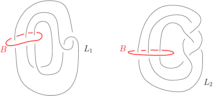
Example 1: See Figure 1 for the diagram. Here $\mathbb{L}$ is an unknot in $S^{3}$, so $\widetilde{B}$ is a knot in $S^{3}$ as well. Untwisting and taking the branched double cover (or using symmetry between the two components) shows that $\widetilde{B}$ is the knot:

This is the alternating knot, $6_{1}$, with signature equal to $0$. The main result in [9] now verifies the knot Floer conclusions of theorem 3.1. We note for later that the Alexander polynomial is $-2\,T^{-1}+5-2\,T$.

Example 2: See Figure 1 for the diagram. Here $\mathbb{L}$ is the figure-8 knot, $4_{1}$, whose branched double cover is $L(5,2)$. In this arrangement, $\widetilde{B}$ is a genus $1$ fibered knot in $L(5,2)$. The possibilities for the homology of such a knot are strictly limited, since there is only a $\mathbb{Z}$ in filtration levels $\pm 1$. The real content of the theorem here is that $\tau(\widetilde{B})=0$, as this implies that there is one $Spin^{c}$ structure where the knot Floer homology is that of $4_{1}$. We give a non genus $1$ example later.

The monodromy for this knot is $\big(\gamma_{1}\gamma_{2}^{-1}\big)^{2}$ where $\gamma_{i}$ is a positive Dehn twist around a standard symplectic basis element for $H_{1}(T^{2}-D^{2})$. The monodromy action on $H_{1}$ and the Alexander polynomial associated to the $\mathbb{Z}$-covering from the fibering are computed to be

$$A=\left[\begin{array}[]{cc}2&3\\ 3&5\\ \end{array}\right]\hskip 36.135pt\Longrightarrow\hskip 36.135pt\mathrm{det}(I-tA)\doteq\Delta_{\widetilde{B}}(t)=-T^{-1}+7-T^{1}$$

where we have symmetrized and normalized $\mathrm{det}(I-tA)$ according to our convention. In fact we should use the more refined torsion, $\check{\tau}(Y-K)$, in our Euler characteristic computations, [4]. This we now proceed to calculate.

The fundamental group of $\Sigma(\mathbb{L})-\widetilde{B}$ can be computed using the basis for $\pi_{1}(F)$ above. The action of $(D_{\gamma_{1}}D_{\gamma_{2}}^{-1})^{2}$ on the two elements generating this free group is

$$\begin{array}[]{l}\gamma_{1}\longrightarrow\gamma_{1}\gamma_{2}\gamma_{1}^{2}\gamma_{2}\gamma_{1}\gamma_{2}\gamma_{1}=R(\gamma_{1})\\ \\ \gamma_{2}\longrightarrow\gamma_{1}\gamma_{2}\gamma_{1}^{2}\gamma_{2}=R(\gamma_{2})\end{array}$$

These provide the relations $\gamma_{1}^{-1}tR(\gamma_{1})t^{-1}$ and $\gamma_{2}^{-1}tR(\gamma_{2})t^{-1}$ for the fundamental group.

For the choice above, we obtain the map on homology $e_{1}\rightarrow 5e_{1}+3e_{2}$ and $e_{2}\rightarrow 3e_{1}+2e_{2}$. The quotient $\mathbb{Z}^{2}/(I-A)$ has a basis given by $(5,0)$ and $(3,1)$. The map to $H_{1}(\Sigma(\mathbb{L}))$ is thereby given as $\gamma_{1}\rightarrow e$ and $\gamma_{2}\rightarrow e^{-3}$ (switching to exponents) with $e^{5}=0$. We now apply Fox calculus to the relations, and then map to $H_{1}(\Sigma(\mathbb{L})-\widetilde{B})$ using the previous map and $t\rightarrow T$. We illustrate with one calculation:

$$(\rho\otimes\epsilon)(\partial_{\gamma_{2}}\,R_{1})=(\rho\otimes\epsilon)(\gamma_{1}^{-1}t\big(\gamma_{1}+\gamma_{1}\gamma_{2}\gamma_{1}^{2}+\gamma_{1}\gamma_{2}\gamma_{1}^{2}\gamma_{2}\gamma_{1}\big))$$

$$=e^{-1}t(e+e\cdot e^{-3}\cdot e^{2}+e^{-2})=t(1+e^{4}+e^{2})$$

The overall matrix (removing the column for the derivatives related to $t$) is

$$\left[\begin{array}[]{cc}-e^{4}+T(2e^{4}+e+e^{2}+e^{3})&T(1+e^{2}+e^{4})\\ T(e+e^{2}+e^{3})&-e^{3}+T(e^{3}+e^{4})\\ \end{array}\right]$$

which has determinant $-T-T\,e+(1-3T+T^{2})e^{2}-T\,e^{3}-T\,e^{4}$. Symmetrizing in $T$ produces the correct Euler characteristic up to signs. This determines the ranks in each of the filtration indices for each of the $Spin^{c}$ structures.

This fibered knot can also be seen by surgery on the diagram for $B(0,0)$ as in Figure 2. The box around $+3$ indicates that we will use it for the surgery sequence with framings $\infty,+2,+3$. For $\infty$ we obtain a knot in $L(2,1)$ identical with $B(-1,2)$. For $+2$ surgery we obtain the unknot in $L(-3,1)$. Since $L(5,2)$ has five $Spin^{c}$ structures, the sequence for the $\widehat{HFK}$ splits (all the homology from $L(-3,1)$ must map to that for the fibered knot in $L(5,2)$). The knot $B(-2,1)$ has homology $\mathbb{Z}$ in filtration level $0$ for one $Spin^{c}$ structure, and homology identical with $\widehat{HFK}(4_{1})$ in the other. This follows from a Borromean rings calculation or can be found in [5]. Thus all the terms in filtrations other than $0$ should occur for a single $Spin^{c}$ structure (the one fixed under conjugation).

Example 3: Consider the situation in section 5.2 of [5]: a genus 1 fibered knot with monodromy $D_{\gamma_{1}}^{n}D_{\gamma_{2}}^{m}$ with $m\cdot n<0$. This is the branched double cover of the closure of the three stranded braid $\sigma_{1}^{n}\sigma_{2}^{m}$. Assume for now that $m<0$. Then the action of the monodromy on $H_{1}(F)$ is given by

In [3] E. Eftekhary proves the following theorem for the Floer cohomology of symplectomorphisms:

References

- [1] M. Asaeda, J. Przytycki, & A. Sikora, Categorification of the Kauffman bracket skein module of -bundles over surfaces. Alg. & Geom. Top. 4:1177-1210 (2004).
- [2] A. Champanerkar & I. Kofman, Spanning Trees and Khovanov homology. math.GT/0607510 v1
- [3] E. Eftekhary, Floer cohomology of certain pseudo-Anosov maps. math.SG/0205029 v3
- [4] J. E. Grigsby, Knot Floer homology in cyclic branched covers. Alg. & Geom. Top. 6:1355–1398 (2006).
- [5] S. Jabuka & T. Mark, Heegaard Floer homology of certain mapping tori. Alg. & Geom. Top. 4:685-719 (2004)
- [6] E. S. Lee, An endomorphism of the Khovanov invariant. Adv. Math. 197(2): 554-586 (2005).
- [7] C. Livingston, Computations of the Ozsváth-Szabó knot concordance invariant. Geo. & Top. 8:735-742 (2004).
- [8] Y. Ni, Sutured Heegaard diagrams for knots. math.GT/0507440v1
- [9] P. Ozsváth & Z. Szabó, Heegaard-Floer Homology and Alternating Knots. Geom. Topo. 7:225-254 (2003).
- [10] P. Ozsváth & Z. Szabó, Heegaard Floer homology and contact structures. Duke Math. J. 129(1): 39-61 (2005).
- [11] P. Ozsváth & Z. Szabó, Holomorphic disks and knot invariants. Adv. Math., 186(1): 58-116 (2004).
- [12] P. Ozsváth & Z. Szabó, On the Heegaard Floer homology of branched double covers. Adv. Math. 194(1): 1-33 (2005).
- [13] R. C. Penner, A construction of pseudo-Anosov homeomorphisms. Trans. Amer. Math. Soc. 310(1): 179-197 (1988).
- [14] L. Roberts, On knot Floer homology in double branched covers. math.GT/??
- [15] S. Wehrli, A spanning tree model for Khovanov homology. math.GT/0409328 v2