Characterizing dynamics with covariant Lyapunov vectors
Abstract
A general method to determine covariant Lyapunov vectors in both discrete- and continuous-time dynamical systems is introduced. This allows to address fundamental questions such as the degree of hyperbolicity, which can be quantified in terms of the transversality of these intrinsic vectors. For spatially extended systems, the covariant Lyapunov vectors have localization properties and spatial Fourier spectra qualitatively different from those composing the orthonormalized basis obtained in the standard procedure used to calculate the Lyapunov exponents.
pacs
05.70.Ln,87.18.Ed,45.70.-nMeasuring Lyapunov exponents (LEs) is a central issue in the investigation of chaotic dynamical systems because they are intrinsic observables that allow to quantify a number of different physical properties such as sensitivity to initial conditions, local entropy production and attractor dimension review. Moreover, in the context of spatiotemporal chaos, the very existence of a well-defined Lyapunov spectrum in the thermodynamic limit is a proof of the extensivity of chaos ext_chaos, and it has been speculated that the small exponents contain information on the “hydrodynamic” modes of the dynamics (e.g., see ecpo and references therein).
In this latter perspective, a growing interest has been devoted not only to the LEs but also to some corresponding vectors, with the motivation that they could contribute to identifying both the real-space structure of collective modes Demonte and the regions characterized by stronger/weaker instabilities egolf. However, the only available approach so far is based on the vectors yielded by the standard procedure used to calculate the LEs benettin. This allows to identify the most expanding subspaces, but has the drawback that these vectors —that we shall call Gram-Schmidt vectors (GSV) after the procedure used— are, by construction, orthogonal, even where stable and unstable manifolds are nearly tangent. Moreover, GSV are not invariant under time reversal, and they are not covariant, i.e. the GSV at a given phase-space point are not mapped by the linearized dynamics into the GSV of the forward images of this point.
While the existence, for invertible dynamics, of a coordinate-independent, local decomposition of phase space into covariant Lyapunov directions —the so-called Oseledec splitting review— has been discussed by Ruelle long ago Ruelle, it received almost no attention in the literature, because of the absence of algorithms to practically determine it. In this Letter, we propose an innovative approach based on both forward and backward iterations of the tangent dynamics, which allows determining a set of directions at each point of phase space that are invariant under time reversal and covariant with the dynamics. We argue that, for any invertible dynamical system, the intrinsic tangent space decomposition introduced by these covariant Lyapunov vectors (CLV) coincides with the Oseledec splitting.
As a first important and general application of the CLV, we show that they allow to quantify the degree of hyperbolicity of the dynamics. Considering that all physically relevant dynamical systems are not hyperbolic (i.e. stable and unstable manifolds are not everywhere transversal), and that many of the available theoretical results have been derived under the assumption of strict hyperbolicity (a prominent example being the Gallavotti-Cohen fluctuation theorem gallavotticohen), it is indeed highly desirable to develop a tool to quantify deviations from hyperbolicity. At the moment, this is doable only in very simple systems such as the Hénon map or the Duffing oscillator, where homoclinic tangencies can be detected by iterating separately the tangent dynamics forward and backward in time. Since CLV correspond to the local expanding/contracting directions, we can straightforwardly evaluate their relative transversality and, accordingly, quantify the degree of hyperbolicity. Note that GSV, being mutually orthogonal, are useless in this context. In a second important application of CLV we show that, contrary to the weak localization of GSV, they are generically localized in physical space, providing an intrinsic, hierarchical decomposition of spatiotemporal chaos. Furthermore, the knowledge of CLV paves the way to analytical methods for determining the LEs as ensemble- rather than time-averages.
Description of the algorithm. We first summarize the standard method for computing the LEs (we consider, for simplicity, a -dimensional discrete-time dynamical system). Let denote the phase-space point at time and let , , be the orthogonal vectors obtained by applying the Gram-Schmidt orthogonalization procedure to tangent-space vectors (we shall call this the th GS basis). Iterating the evolution equations once, is transformed into , where is the Jacobian of the transformation evaluated at time . The th GS basis is thereby obtained by applying the Gram-Schmidt transformation to the vectors . This amounts to computing the so-called QR decomposition of the matrix whose columns are the Jacobian-iterated vectors of the th GS basis: . The th GS basis is given by the columns of the orthogonal matrix , while is an upper-triangular matrix whose off-diagonal nonzero elements are obtained by projecting each vector onto the subspace spanned by with . It has been shown ershovpotapov that, by repeating the above procedure up to a time for much larger than , the GS basis converges to an orthogonal set of vectors , - the th Gram-Schmidt vectors - which solely depend on the phase space point .
The LEs are then nothing but the time-averaged values of the logarithms of the diagonal elements of . The method we propose also exploits the usually disregarded information contained in the off-diagonal elements. Let us now assume that a set of GSV has been generated by iterating the generic initial condition . Let be a generic vector inside the subspace spanned by , , i.e. the first GSV at time . We now iterate this vector backward in time by inverting the upper-triangular matrix : if the are the coefficients expressing it in terms of the GSV in , one has , where is a matrix element of . Since is upper-triangular, it is easy to verify that at all times . This is due to the fact that is a covariant subspace. Iterating backward for a sufficiently large number of times, it eventually aligns with the (backward) most expanding direction within . This defines , our intrinsic -th (forward) expanding direction at the phase-space point . It is straightforward to verify that is covariant. Define the matrix ; then one has . By multiplying both sides by and substituting for its QR decomposition on the resulting right hand side, one is simply left with for . The CLV are independent of where the backward evolution is started along a given trajectory, provided that it is sufficiently far in the future. Moreover, we have verified that they are invariant under time reversal, i.e. that the direction of is the same whether we first move backward along a given trajectory (applying the standard orthonormalization procedure) and then forward (according to the above outlined methodology).
Our CLV thus constitute an intrinsic, covariant basis defining expanding/contracting directions in phase space NOTE. The LEs are simply obtained from the CLV: the th exponent is the average of the growth rate of the th vector yanchuk. We have checked on simple invertible maps that they coincide with the Oseledec splitting in . We conjecture that this is the case for any invertible system. Note that our CLV are also well defined for non-invertible dynamics, since it is necessary and sufficient to follow backward a trajectory previously generated forward in time. In this respect they provide an extension of the Oseledec splitting. Finally, and retrospectively, a preliminary evidence of the validity of our approach was given in PTL, where CLV were introduced to characterize time periodic orbits in a 1D lattice of coupled maps. There, it was found that the number of nodes (changes of sign) in a CLV is directly connected to the position of the corresponding LE within the Lyapunov spectrum.
We stress that the determination of the CLV can be very efficient, making them a truly practical tool (as opposed, say, to calculating directly the Oseledec splitting in the case of invertible dynamics). Indeed, the major computational bottleneck is the memory required to store the matrices and the -time GSV during the forward integration. This difficulty can be substantially reduced by occasionally storing the instantaneous configuration in real and tangent space and re-generating the rest when needed.
Numerical analysis. We measured the CLV in four one-dimensional systems made of nonlinear units coupled to their nearest neighbors. Periodic boundary conditions are used. The first is a chain of chaotic tent maps (TM) on the unit interval,
| (1) |
In the following we fix and .
The second system is a chain of symplectic maps (SM),
| (2) |
where . This model was studied in RadonsMap to analyse the so-called “hydrodynamic Lyapunov modes”. Eq. (2) conserves total momentum , and is invariant under a translation of the coordinates. Therefore, the Lyapunov spectrum possesses two null exponents. In the following we fix .
The last two models are second-order continuous-time systems governed by
| (3) |
For , we have the rotator model (RM), while for , the system reduces to a Fermi Pasta Ulam chain (FPU). These two widely studied Hamiltonian systems provide a good testing ground to investigate the connection between microscopic dynamics and statistical mechanics. Besides the zero LE associated with a shift along the trajectory, both models have three other null LEs arising from energy and momentum conservation plus translational invariance. Numerical simulations have been performed at energy density (for the RM) and (for FPU).

Hyperbolicity. A dynamical system is said to be hyperbolic if its phase space has no homoclinic tangencies, i.e. the stable and unstable manifolds are everywhere transversal to each other. In the mathematical literature, it is known that the Oseledec splitting is connected to hyperbolicity Bochi, but the lack of practical algorithms to determine the splitting makes such results of little use in physically relevant contexts. Here, the knowledge of the CLV allows testing hyperbolicity by determining the angle between each pair of expanding () and contracting () directions
| (4) |
where the absolute value is taken because signs are irrelevant. As a first test, we have computed the probability distribution of for two classic two-dimensional maps. Arbitrarily small angles are found for the Hénon map, while the distribution is bounded away from zero in the Lozi map (Fig. 1a). This is perfectly consistent with the well-known fact that only the latter model is hyperbolic Collet.
In spatially extended systems, given the multi-dimensional character of the invariant manifolds, it is appropriate to determine the minimum angle, where are the expanding and contracting invariant subbundles at time along the trajectory. The histograms in Fig. 1b show that models (1) and (2) are characterized by stronger hyperbolicity violations than the Hamiltonian systems. Altogether, recalling that refers to the least transversal pair of directions, we are led to conclude that the dynamics of high-dimensional systems should be closer to hyperbolic than that of low-dimensional ones. This justifies the often-made assumption that spatially-extended systems are practically hyperbolic.
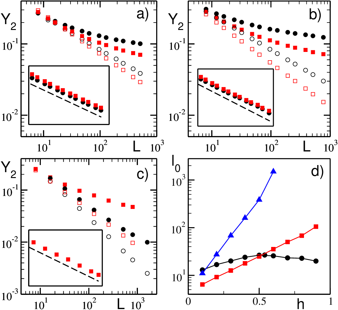
Localization properties in extended systems. The spatial structure of the vectors associated to the LEs is of interest in many contexts. We now show that the GSV —which have been used so far— and the CLV have qualitatively different localization properties. One usually considers the inverse participation ratio part where indicates an average over the trajectory and is a measure of the component of the th vector at site (with the normalization ). In systems characterized by a single local real variable (such as our TM), is taken to be the -th component of the -th CLV or GSV, while in the case of symplectic systems, where two components are present (), it is natural to choose . In order to investigate the thermodynamic limit, it is necessary to determine for fixed and increasing . On the one hand, localized vectors are characterized by a finite inverse participation ratio, , for , where is a localization “length”. On the other hand, in completely delocalized structures, .
In Fig. 2 we show how typically scales with the chain length . The GSV show weak (de)localization: their participation ratio exibits an -dependent “dimension” : . One can show that this anomalous behavior is entirely due to the Gram-Schmidt procedure, and has nothing to do with the dynamics unpublished. On the other hand, CLV are localized objects. For TM, SM and RM dynamics we find good evidence of the scaling law with . This allows for a reliable determination of . For the FPU dynamics, we find only slight curvature in the log-log plot of Fig. 2c, signalling that larger system sizes are probably needed to definitely enter the scaling regime. Moreover, for symplectic dynamics the localization length diverges as (Fig. 2d). Assuming the continuity of the LE spectrum, the divergence of is not surprising, since the conservation laws imply that the Lyapunov vectors (both GSV and CLV) corresponding to (i.e. to null LEs) are completely delocalized.

Fourier analysis. Another way proposed to characterize the spatial structure of a Lyapunov vector is to look at its power spectrum , where denotes the vector component associated with the space coordinate at site . For instance, this was used in RadonsMap in the context of the investigation of so-called “hydrodynamic” modes (only GSV were considered there). Here, we have focused on the vector corresponding to the smallest positive LE in our symplectic models, for which this LE goes continuously to zero as the system size increases (note that GSV and CLV coincide for the null exponents linked to symmetries and conservation laws). We observe again a clear qualitative difference between the spectra of GSV and CLV (Fig. 3). In particular, the near-zero CLV exhibit an intriguing low-frequency divergence of the type in all three symplectic models we have analysed. Thus, the qualitative difference between GSV and CLV extends to the case.
Perspectives. Now that the local directions of stable and unstable manifolds are made available in generic models, many questions can be addressed in a more accurate way: Quantifying (non-)hyperbolicity in the context of the (numerical) attempts to “verify” the fluctuation theorem is one. Another set of questions relates to the spatial structure of the dynamics in extended systems, such as the quantification of local degree of chaos (amount of instability), a hierarchical decomposition of spatiotemporal chaos, the search for true, intrinsic, collective (“hydrodynamic”) modes, etc. A further field where the knowledge of CLV can help to make progress is optimal forecast in nonlinear models. Here the knowledge of the local transversality of the invariant manifolds can indeed be combined with the so-called bred vectors to use the information on the past evolution to decrease the uncertainty along unstable directions bred.
Acknowledgements.
References
- (1) J.-P. Eckmann and D. Ruelle, Rev. Mod. Phys. 57 617 (1985).
- (2) D. Ruelle, Thermodynamic Formalism, Reading, MA: Addison & Wesley (1978); R. Livi, A. Politi and S. Ruffo, J. Phys. A 19, 2033 (1986); P. Grassberger, Phys. Scri. 40, 346 (1989).
- (3) J.-P. Eckmann, C. Forster, H.A. Posch and E. Zabey, J. Stat. Phys 118, 813 (2005).
- (4) N. Nakagawa and Y. Kuramoto, Physica D 80, 307 (1995); S. De Monte, F. d’Ovidio, H. Chaté and E. Mosekilde, Phys. Rev. Lett. 92, 254101 (2004).
- (5) K. Kaneko, Physica D, 23, 436 (1986); H. Chaté, Europhys. Lett. 21 419, (1993); D.A. Egolf, E.V. Melnikov, W. Pesch and R.E. Ecke, Nature, 404, 733 (2000).
- (6) I. Shimada and T. Nagashima, Prog. Theor. Phys. 61, 1605 (1979); G. Benettin, L. Galgani, A. Giorgili, and J.M. Strelcyn, Meccanica, 15, 21 (1980).
- (7) D. Ruelle, Publ. Math. IHES 50, 275 (1979).
- (8) G. Gallavotti and E.G.D. Cohen, Phys. Rev. Lett. 74, 2694 (1995).
- (9) S.V. Ershov, A.B. Potapov, Physica D 118, 167 (1998).
- (10) We expect that the CLV are ill-defined in the presence of degeneracies; in such cases, they have to be grouped according to the multiplicity of the corresponding LE.
- (11) As it has been shown for simple 2D maps and 3D smooth flows: B. Eckhardt, D. Yao, Phyisica D 65, 100 (1993); G. Froyland, K. Judd and A. I. Mees, Phys. Rev. E 51, 2844 (1995); A. Politi, F. Ginelli, S. Yanchuk, and Yu. Maistrenko, Physica D, 224 90 (2006).
- (12) A. Politi, A. Torcini, S. Lepri, J. Phys. IV 8, 263 (1998).
- (13) H. Yang and G. Radons, Phys. Rev. E 73, 016202 (2006).
- (14) Ya. B. Pesin, Russian Math. Surveys 32, 55 (1977); J. Bochi, M. Viana, Ann. I.H. Poincaré 19, 113 (2002).
- (15) More precisely, the Lozi map is hyperbolic with the exception of a zero measure set of cuspidal points where the tangent bundle is not defined: P. Collet and Y. Levy, Commun. Math. Phys. 93, 461 (1984).
- (16) A. D. Mirlin, Phys. Rep. 326, 259 (2000).
- (17) J. Kockelkoren and H. Chaté, unpublished.
- (18) D. Patil et al., Phys. Rev. Lett. 86, 5878 (2001).