Sampling Colourings of the Triangular Lattice
Abstract
We show that the Glauber dynamics on proper 9-colourings of the triangular lattice is rapidly mixing, which allows for efficient sampling. Consequently, there is a fully polynomial randomised approximation scheme (FPRAS) for counting proper 9-colourings of the triangular lattice. Proper colourings correspond to configurations in the zero-temperature anti-ferromagnetic Potts model. We show that the spin system consisting of proper 9-colourings of the triangular lattice has strong spatial mixing. This implies that there is a unique infinite-volume Gibbs distribution, which is an important property studied in statistical physics. Our results build on previous work by Goldberg, Martin and Paterson, who showed similar results for 10 colours on the triangular lattice. Their work was preceded by Salas and Sokal’s 11-colour result. Both proofs rely on computational assistance, and so does our 9-colour proof. We have used a randomised heuristic to guide us towards rigourous results.
1 Introduction
This paper is concerned with proper 9-colourings of the triangular lattice. A -colouring of a graph is an assignment of colours from the set to the vertices. A colouring is proper if adjacent vertices receive different colours. There are two fundamental problems that have been studied extensively: sampling -colourings from the uniform distribution on proper -colourings of and counting the number of proper -colourings of . Both these problems have been studied for various graphs and number of colours, and it has been shown that the two problems are intimately related. More precisely, if there is an efficient method of finding a good approximate solution to one of the problems, then there is an efficient method of finding a good approximate solution to the other problem. See for instance [14] and [15] for details on this topic. The problem of counting -colourings of a graph with maximum degree is -complete when and (see [3]). Hence we have to rely on approximate solutions. A great deal of work has been put into mapping out for which graphs and number of colours there is a fully polynomial randomised approximation scheme (FPRAS) for counting colourings, or equivalently, a fully polynomial almost uniform sampler (FPAUS).
Sampling colourings is closely related to problems arising in statistical physics, where proper colourings correspond to configurations in the zero-temperature anti-ferromagnetic Potts model. The notion of a proper colouring imposes a very local property: it constrains the allowed colours on two adjacent vertices. Given local constraints, physicists are interested in understanding the macroscopic properties of the system.
Let be an infinite graph. Think of as lattice graph, for example the grid. For a finite subgraph of , the boundary of is the set of vertices in that are adjacent to but are not in themselves. Given a colouring of the boundary, a proper -colouring of agrees with if no vertex adjacent to the boundary receives any of the colours of its boundary neighbours. Let denote the uniform distribution on proper -colourings of that agree with . Suppose is a distribution on the set of proper -colourings of the infinite graph . For a proper -colouring of , let denote the conditional distribution on proper -colouring of induced by when the colours of all vertices except for those in are specified by . The distribution is an infinite-volume Gibbs distribution (with respect to proper colourings) if, for any proper -colouring of , , where is the colouring of the boundary of induced by . That is, the conditional distribution on colourings of depends only on the boundary of and not on other vertices of . The physical intuition for an infinite-volume Gibbs distribution is that it describes a macroscopic equilibrium, for which all parts of the system are in equilibrium with their boundaries. It is known that there always exists at least one infinite-volume Gibbs distribution [7], and a central question in statistical physics is to determine whether it is unique or not. The phenomenon of non-uniqueness is referred to as a phase transition. For more on Gibbs distributions, see, for example, [6] or [7].
Given a finite subgraph of and a boundary colouring of , let be any connected subset of the vertices of and let be the distribution on colourings of that is induced by . The question we ask is how does change if we change the colour of one single vertex on the boundary of . If is far away from the boundary then we would expect that changing the colour of a boundary vertex does not have too much influence on . If this is true, then we have a property known as strong spatial mixing. The exact definition will be given later. A consequence of strong spatial mixing is that the infinite-volume Gibbs distribution is unique [5, 21, 22]. In this paper we show that there is strong spatial mixing for 9 colours on the triangular lattice.
Another important problem in statistical physics is to determine how quickly a system converges to equilibrium. This could lead to insights in how the system returns to equilibrium after a shock has disturbed it. A dynamical process that is commonly studied is the Glauber dynamics. The Glauber dynamics is a Markov chain on the set of proper -colourings of a graph . A transition from one state (colouring) to another is made as follows. Choose a vertex uniformly at random and choose one of the colours uniformly at random. If the randomly selected colour is different from the colours of the neighbours of then recolour with the selected colour. This procedure is also known as a single-vertex heat-bath update. If it is repeated over and over then the distribution of the current state of the Markov chain will converge towards the uniform distribution. The question is how long to run the dynamics in order to get close to the uniform distribution. If we only need to simulate the dynamics over a small number of steps then the Glauber dynamics would be a suitable tool for sampling colourings. We say that a Markov chain is rapidly mixing if a small number of steps are sufficient in order to get arbitrarily close to its stationary distribution. Exact definitions will be given later. It is a well-known fact that if the system has strong spatial mixing, then the Glauber dynamics is (often) rapidly mixing [5, 16, 21]. In fact, the converse is also true. Since we prove strong spatial mixing for 9 colours on the triangular lattice, we also prove that the Glauber dynamics is rapidly mixing. That is, we show that there is an FPAUS for sampling 9-colourings of the triangular lattice. As mentioned above, the FPAUS implies that there is an FPRAS for counting 9-colourings.
1.1 Organisation
The remainder of the paper is organised as follows. In Section 2, we define the basic notation, strong spatial mixing and the Glauber dynamics. In Section 3, we formally state our results and discuss related work. In Section 4, we introduce two key concepts that will be used throughout the paper, and Sections 5 through 6 contain the technical part that leads to the strong spatial mixing result. Section 7 is about the implication from strong spatial mixing to a rapidly mixing Glauber dynamics. Finally, in Section 8, we describe the computer assisted parts of our proofs.
2 Preliminaries
2.1 Basic notation
Let the infinite graph denote the triangular lattice, formally defined as follows. There is a bijection from to and is even} such that has the six neighbours , , , , and . Note that maps a vertex of to a coordinate in a Cartesian coordinate system, which allows us to draw the triangular lattice as illustrated in Figure 2. However, throughout this article we will draw vertices as a hexagons, illustrated in Figure 2.
The bijection specifies a unique clockwise ordering of edges incident to the same vertex. We write to indicate that is the clockwise ordering of the edges around some vertex . We say that two edges and incident to the same vertex are clockwise adjacent if either or , where are the other four edges in incident to .
A region is a finite subset of and its edge boundary, denoted . The vertex boundary of , denoted .
For a region , and , we let denote the number of edges on a shortest path in between and such that all vertices in except for are in . Thus, if and are adjacent. For a subregion , we let .
Let . A -colouring of a set (a set of vertices or edges), is a function from to , where represents a set of colours. A partial -colouring of is a function from to , where the additional colour 0 can be thought of as representing “no colour.”
A -colouring of a region is proper if for all , when . For a partial -colouring of the boundary , a -colouring of agrees with if for all , . Similarly, for a partial -colouring of , a -colouring of agrees with if for all , . To aid the reader, we use the calligraphic font to represent colourings of vertices and the normal font to represent colourings of edges (like and above). Further, partial colourings (containing the “colour” 0) are used only for boundary vertices and boundary edges and not for the regions themselves.
For a region and partial -colouring of (respectively, of ), (respectively, ) denotes the set of proper -colourings of that agree with (respectively, ). The uniform distribution on (respectively, ) is denoted (respectively, ). For a subregion , we let denote the distribution on proper -colourings of induced by .
For a distribution on a set , we write for the probability of drawing under . The total variation distance between two distributions and on a set is
For two distributions and on two sets and , respectively, a coupling of and is a joint distribution on that has and as its marginal distributions.
We write to denote the expected value of a random variable .
2.2 Strong spatial mixing
We say that there is strong spatial mixing for colours on the triangular lattice if there are two constants (that may depend on ) such that
| (1) |
is true for all regions , subregions , and partial -colourings and of such that for all , , and .
2.3 The Glauber dynamics
The Glauber dynamics for -colourings of a region with partial -colouring of is a Markov chain with state space and the following transitions. The evolution from a colouring to a new colouring is defined by the following steps.
- 1.
Choose a vertex from uniformly at random.
-
Let be the colouring of specified by and .
-
Let .
- 2.
Choose a colour from uniformly at random.
- 3.
Let
The probability of not leaving a state in a transition is always positive. Hence the Glauber dynamics is an ergodic Markov chain if the number of colours is sufficiently large; every state can be reached from any other state. In this article we are concerned with colours for which we note that there are always at least three available colours in Step 2 of the dynamics above. Hence the Glauber dynamics is ergodic for .
It is straightforward to verify that when the Glauber dynamics is ergodic then its stationary distribution is . Let be the distribution on after steps of the Glauber dynamics, starting with colouring . For , the mixing time
is the number of transitions until the dynamics is within total variation distance of the stationary distribution, assuming the worst initial colouring . We say that the Glauber dynamics is rapidly mixing if is upper-bounded by a polynomial in and .
2.4 Approximate counting
A randomised approximation scheme (RAS) for a function is a probabilistic Turing machine that takes as input a pair , and produces, on an output tape, an integer random variable satisfying the condition . The choice of the value is inconsequential: the same class of problems has a RAS if we choose any probability in the interval (see for example [15]). A fully polynomial randomised approximation scheme (FPRAS) is a RAS that runs in time upper-bounded by a polynomial in and .
It was mentioned in the introduction that the existence of an efficient method for sampling colourings implies that there is an FPRAS for counting the number of colourings. We could use a rapidly mixing Glauber dynamics to construct (in a non-trivial way) an FPRAS for estimating . For details on the topic of how sampling and counting are related, see, for example, [14] or [15].
3 Our results and related work
These are the two main theorems of the paper.
Theorem 1.
There is strong spatial mixing for 9 colours on the triangular lattice.
Theorem 2.
The Glauber dynamics on 9-colourings of a region of the triangular lattice, with partial 9-colouring of , has mixing time , where .
The previously best known mixing results on the triangular lattice was given for 11 colours by Salas and Sokal [19] in 1997, and later improved by Goldberg, Martin and Paterson [9] to 10 colours in 2004. Both proofs involved computational assistance.
To place these results in context, we first mention some general mixing bounds that are applicable to graphs with small girth, such as many of those lattices studied in statistical physics. Independently, Jerrum [13] and Salas and Sokal [19] proved that for proper -colourings on a graph of maximum degree , the Glauber dynamics has mixing time when , where is the number of vertices. For , Bubley and Dyer [2] showed that it mixes in time, and later Molloy [17] showed that it mixes in time. In [20], Vigoda used a Markov chain that differs from the Glauber dynamics and showed that it has mixing time when . This result implies that also the Glauber dynamics is rapidly mixing for . Goldberg, Martin and Paterson [9] showed that any triangle free graph has strong spatial mixing provided , where is the solution to () and . For triangle free graphs of low degree, this is still today the best general mixing bound that has been proved.
The technique Goldberg, Martin and Paterson used in [9] can be tailored and tweaked for particular graphs in order to give mixing bounds that are better than the general bound. This was demonstrated in [9] for the lattice with colours (the general result would give mixing for colours), and the triangular lattice with colours. Although the general result holds only when the graph is triangle free, the tailored proof for the triangular lattice does not require this. Both proofs were computer assisted, where the computational part consisted of looping though a huge number of boundary colourings and maximising certain values. This task would have been impossible to do by hand.
The general mixing bounds are tough barriers that seem difficult to break, though in many cases we expect mixing to occur with fewer colours. Therefore several proofs of mixing have been given for specific graphs or lattices. These proofs often involve computational assistance. We have mentioned two examples above as well as Salas and Sokal’s 11-colour mixing bound on the triangular lattice [19]. Other examples of computer assisted proofs are those by Achlioptas, Molloy, Moore and van Bussel [1], who showed mixing for colours on the grid, to which an alternative proof was given by Goldberg, Jalsenius, Martin and Paterson in [8]. Salas and Sokal gave in [19] a computer assisted proof for colours on the kagome lattice, which was later improved to colours by Jalsenius in [11]. It should also be mentioned that Jalsenius and Pedersen [12] have given a computer assisted proof of mixing with colours for the grid when the dynamics is updating vertices in deterministic order, as opposed to the Glauber dynamics which chooses a vertex at random in each step. The new colour is still chosen at random, though. This result is an improvement of the non-computer assisted proofs by Pedersen [18] and Dyer, Goldberg and Jerrum [4].
The results on 9-colourings of the triangular lattice that we present in this paper are based on the 10-colour proof given by Goldberg, Martin and Paterson in [9]. Our 9-colour proof is of a whole different scale than the 10-colour proof and we must use computer assistance much more extensively and in more than one stage of the proof. The computations are rather demanding and prior to the final and rigourous results we had to use a heuristic to guide us in the right direction. We believe that the idea of such a heuristic could be useful to improve the mixing bounds for other lattices as well. However, our proof also demonstrates how demanding the computations can be, and unless new techniques are developed, there will probably be little progress in lowering the bounds for a vast number of lattices.
4 Boundary pairs
Similarly to Goldberg, Martin and Paterson in [9], we define two structures referred to as vertex-boundary pairs and edge-boundary pairs. Before stating the formal definitions, we give an overview of the two concepts. A vertex-boundary pair consists of a region and two partial colourings of its vertex boundary. The colourings are identical except for on one boundary vertex, which is not allowed to have the colour 0 in either of the two colourings. That is, the vertex must have a “real” colour. An edge-boundary pair is similar to a vertex-boundary pair with the difference that the two boundary colourings are of the edge boundary instead of the vertex boundary. The formal definition of an edge-boundary pair might come across as slightly awkward as there are some additional conditions that must be met. The purpose of these conditions is to facilitate certain technicalities in the subsequent sections.
Formally, a vertex-boundary pair consists of
- •
a region ,
- •
a distinguished boundary vertex and
- •
a pair of partial 9-colourings of such that
- –
for all , and
- –
and .
- –
An edge-boundary pair consists of
- •
a region ,
- •
a distinguished boundary edge , where and are two distinguished vertices such that at most five neighbours of are in , and
- •
a pair of partial 9-colourings of such that
- –
for all , ,
- –
, , and
- –
for any two clockwise adjacent edges that share a vertex , or .
- –
Note that the very last condition means that two clockwise adjacent edges have the same colour in both and unless one of the edges is .
We let denote the set of edges between and a vertex in .
For a vertex-boundary pair (or edge-boundary pair ), a coupling of and (or and ) and , we define the indicator random variable
For an edge-boundary pair , we define to be some coupling of and minimising . We define . For every pair of colours, we let be the probability that, when a pair of colourings is drawn from , and . Note that
5 Recursive coupling
In order to show strong spatial mixing for colours, we show that for all vertex-boundary pairs and subregions , there exists a coupling of and such that
decreases exponentially in the distance between and . As we will see, this implies strong spatial mixing for colours. In order to show exponential decay, it will be convenient to work with edge-boundary pairs.
We closely follow the approach taken by Goldberg, Martin and Paterson in [9] and define a tree associated with each edge-boundary pair . The tree is constructed as follows (Figure 3 illustrates an example of a tree ).
Start with a node which will be the root of . For every pair of colours such that , add an edge labelled from to a new node . If is empty, is a leaf. Otherwise, let be the edges in such that . For each , let be the edge-boundary pair consisting of
- •
the region ,
- •
the distinguished boundary edge , where , and
- •
the pair of partial 9-colourings of such that
- –
for ,
- –
for ,
- –
for , and
- –
is identical to on all edges but for which .
- –
Note that the properties of meet all the requirements for being an edge-boundary pair; the vertex has at most five neighbours in (since is a neighbour of ), and any two clockwise adjacent edges in that share a vertex in have the same colour in or (or both).
Recursively construct , the tree corresponding to edge-boundary pair . Add an edge with label from to the root of . That completes the construction of .
We say that an edge of is degenerate if the second component of its label is ‘’. For edges and of , we write to denote the fact that is an ancestor of . That is, either , or is a proper ancestor of . Define the level of edge to be the number of non-degenerate edges on the path from the root down to, and including, . Suppose that is an edge of with label . We say that the weight of edge is . Also the name of edge is . The likelihood of is . The cost of a vertex in is .
Lemma 3 (Lemma 12 of Goldberg et al. [9]).
For every edge-boundary pair there exists a coupling of and such that, for all , .
In the proof, given by Goldberg, Martin and Paterson in [9], the coupling is constructed recursively in the same manner as the tree . The discrepancy at a given boundary vertex is broken to discrepancies at single boundary edges, so at every stage of the recursion, only pairs of colourings with a discrepancy at a single edge have to be considered (i.e., edge-boundary pairs).
For an edge-boundary pair and , we let denote the set of level- edges in . We define .
Lemma 4.
For every edge-boundary pair and there exists a coupling of and such that
Proof.
By Lemma 3 there is a coupling such that
The following recursive definition of is equivalent to the definition above and will be useful in subsequent sections.
Note that . For a set of edge-boundary pairs, we define . We define for all .
6 Exponential decay
Our first step towards a proof of exponential decay and strong spatial mixing is to show that for any edge-boundary pair , decreases exponentially with . A key ingredient in the proof is the quantity , for which we want to derive sufficiently good upper bounds. This is where we start.
We use the lemma below by Goldberg, Martin and Paterson [9]11 1 In [9], Goldberg, Martin and Paterson define , which is the definition of in this article. They give an alterative definition of , however, as pointed out in the proof of Lemma 13 in [9], their indeed.. The idea is to shrink the region so that is kept within the smaller region, and use this smaller region to construct a new edge-boundary pair whose boundary colourings are identical to the boundary colourings of on overlapping boundary edges. The colours of the boundary edges introduced by shrinking are chosen to maximise . Then .
Lemma 5 (Lemma 13 of Goldberg et al. [9]).
Suppose that is an edge-boundary pair. Let be any subset of which includes . Let be the set of edge-boundary pairs such that , , and, for , and . Then .
In this article, the 39 regions illustrated in Figure 4 are of particular importance to us. In Section 8.2 we discuss why we chose these regions.
 |
 |
 |
|
 |
 |
||
 |
 |
 |
 |
 |
 | ||
 |
 |
 |
 |
Part 1 of 2
 |
 |
 | |
 |
 |
||
 |
 | ||
 |
 |
||
Part 2 of 2
In order to upper-bound for an arbitrary edge-boundary pair , we will shrink the region down to one of the 39 regions and apply Lemma 5. In order to successfully shrink down to match an -region, we might have to consider an appropriate rotation or reflection of the region.
For , we define the constants in Table 1 and prove the following lemma with the help of a computer. Details of the proof are given in Section 8.
Lemma 6.
For , for every edge-boundary pair such that is the region in Figure 4 and and are the vertices labelled and , respectively.
6.1 Regions and sets of edge-boundary pairs
Let be the region in Figure 6, where a vertex and are labelled. Since contains 12 vertices, we define to be the distinct subregions of that all contain the vertex labelled . For , we define to be the set of edge-boundary pairs such that the intersection of and is , where and coincide with the vertices labelled and , respectively. Thus, for any edge-boundary pair , there is a unique such that .
Let be the region in Figure 6, where a vertex and are labelled. The vertex is a “hole” in . We define to be the set of subregions of such that contains and at least one neighbour of is not in . Recall that in the definition of an edge-boundary pair , has at most five neighbours in .
We define a function . Suppose is a region. Then where , are uniquely specified as follows. Let be the set of regions such that (or the reflection of ) is a subregion of , where and coincide with and , respectively. is a region in such that for all . When well defined, are the intersections of and taken according to Figure 7a,…,7f, respectively. If is not well defined then we set . For example, if the vertex above in region (Figure 6) is not in then none of the regions is the intersection of and in Figure 7d, hence .


6.2 Upper bounds
We use a computer to prove the next lemma.
Lemma 7.
The constants in the lemma above have been obtained in the following way. We have written a computer program which goes through the regions of , calculates the values and adds Equation (2) above to a linear program. Once all regions in have been processed, the linear program contains thousands of inequalities. We then use a linear program solver to successfully find a satisfying solution such that each value is in the interval . See Section 8 for more information on the computational part.
Lemma 8.
There exist constants such that, for and , , where .
Proof.
Let be constants satisfying the inequalities in Lemma 7. For , suppose . We use induction on to show that .
For the base case , .
For the inductive step , let be the intersection of and such that and coincide with and , respectively. Hence .
Recall that is the set of edges between and a vertex in . For and such that , let be the edge-boundary pairs defined in the construction of the tree in Section 5. From the definition of , the intersection of and , taken such that and coincide with and , respectively, is , where the value of depends on the edge . Thus, with ,
| (3) |
The next corollary follows immediately from Lemma 8.
Corollary 9.
For every edge-boundary pair and , , where .
Lemma 10.
For every edge-boundary pair and subregion there exists a coupling of and such that
where .
6.3 Vertex-boundary pairs and strong spatial mixing
Similarly to Lemma 10, we prove the following lemma for vertex-boundary pairs.
Lemma 11.
For every vertex-boundary pair and subregion there exists a coupling of and such that
where .
Proof.
Let be any vertex-boundary pair and let . First suppose that has a neighbour . Let be the boundary edges incident to such that . For , let be the edge-boundary pair consisting of
- •
the region ,
- •
the distinguished boundary edge ,
- •
the pair of partial 9-colourings of such that
- –
for , where ,
- –
for ,
- –
and , and
- –
for .
- –
Note that and . Figure 8 illustrates an example of how the edge-boundary pairs are constructed.

We use Lemma 10 and for we let be a coupling of and such that
| (4) |
We define a coupling of and by composing the couplings as follows. Let be pairs of colourings drawn from , respectively. Then is the pair of colourings drawn from . If, for , , then for some . Hence
| (5) |
Lastly, suppose that all neighbours of are in . A technical detail arises here because we can no longer break the discrepancy at into edge-boundary pairs as above. Instead we will first randomly choose a colour of a neighbour of and then define edge-boundary pairs for the region .
Let be any neighbour of and let . We define a coupling of and as follows. Let and be colourings drawn (independently) from and , respectively. Let and be the two colourings of such that and for , and and . Let be a coupling of and which we will define shortly. In a pair of colourings drawn from , the vertex is assigned the colours and , respectively, and the other vertices of are assigned colours according to . It remains to define .
Let be the boundary edges incident to either or such that is incident to , and and . Note that five neighbours of are in and both and are edges between and neighbours of . An example is illustrated in Figure 9.
Similarly to above, we define edge-boundary pairs. For , let be the edge-boundary pair consisting of the region , the distinguished edge and boundary colourings that differ on . Note that and . See Figure 9 for an example.
Let be a coupling of and such that
The in the exponent comes from the fact that for some , the edge is incident to and might be for some .
The coupling is defined by composing the couplings . Thus, with being at most 10,
The main theorem of the paper can now be proved.
Theorem 1.
There is strong spatial mixing for 9 colours on the triangular lattice.
Proof.
Let by any region, , , and and two partial 9-colourings of that are identical on all vertices except for . Suppose that is a coupling of and and let be a pair of colourings drawn from . Then
| (6) |
7 Rapidly mixing Glauber dynamics
We use Theorem 8 of Goldberg, Martin and Paterson [9] to show that the Glauber dynamics is rapidly mixing. Before applying their theorem we must introduce some notation.
Let denote the set of vertices in that are at distance at most from the vertex . Thus we have . From the definition of the triangular lattice it follows that , the number of vertices at distance from , is of order , hence . One can show that but we do not need to be that precise here (see Lemma 2.22 in [10] for a proof). It follows that for all , as . In other words, uniformly in , the “surface-area-to-volume” ratio of balls can be made arbitrarily small with a suitable choice of radius . This property of a graph is known as neighbourhood-amenability.
Goldberg, Martin and Paterson [9] introduced the following definition of an -coupling cover.
Definition 12 (Definition 4 of [9] quoted exactly).
Let denote an infinite graph with maximum degree . Fix . We say that has an -coupling cover if for all vertex-boundary pairs , there is a coupling of and such that
We apply the definition to the triangular lattice. From Lemma 11 it follows that for every vertex-boundary pair there is a coupling of and such that
| (8) |
where is the maximum degree of the triangular lattice and is the appropriate constant. Thus, the triangular lattice has an -coupling cover.
We have the following theorem from [9].
Theorem 13 (Theorem 8 of [9] quoted exactly).
Let denote an infinite neighbourhood-amenable graph with maximum degree . Let be a finite subgraph of with and denote a colouring of using the colours . (We assume that .)
Suppose there exists such that has an -coupling cover. Then the Glauber dynamics Markov chain on is rapidly mixing and .
Since the triangular lattice is neighbourhood-amenable and has an -coupling cover, Theorem 8 of [9] translates directly to our Theorem 2, which is repeated below.
Theorem 2.
The Glauber dynamics on 9-colourings of a region of the triangular lattice, with partial 9-colouring of , has mixing time , where .
8 Computations
In this section we go through the computational steps involved in obtaining the 39 -values from Table 1 and proving Lemma 7. The computations of the -values are rather demanding and took around two weeks to run on a fairly powerful home PC of year 2006. We have used the language C for this task. For proving Lemma 7, we have used the language Python. Details on the implementation is given in Appendix A. The source code is available at http://arxiv.org/abs/0706.0489 .
8.1 Computing the -values from Table 1
Suppose that is an edge-boundary pair. Let be the set of colourings such that , and let be the set of colourings such that . Let be the set of proper 9-colourings of that agree with both and .
Lemma 14.
For any edge-boundary pair X,
Proof.
Recall from the definition of that .
Suppose first that . In order to minimise we construct a coupling of and as follows. Let be a pair of colourings drawn from . If then because is drawn from , preventing from receiving the colour . However, if then we choose , which is always possible under the assumption that . Hence .
Suppose second that . By symmetry we have that . ∎
For each of the 39 regions in Figure 4 we have written a program in C which computes . We use the region to illustrate how is obtained. The other -values are computed similarly.
Let be an edge-boundary pair such that , , , and assign the colours to the boundary edges in , and . See Figure 10.
For , let be the number of proper 9-colourings of that agree with the colouring of the boundary, disregarding the colour of the edge , and assign the colour to . Thus, , and . We write a subroutine that computes the values given the colours . Computing them in a brute force manner will take too long so we must be a little more clever than that. We construct a dynamic programming table which lets us reuse the number of colourings computed for subsets of the region . For details, see Appendix A.
Let be a function of . We loop through the colours , and for each configuration we compute . It follows that is the largest value of that we encounter.
Each colour can take a value from the set . Looping through all configurations of yields an unnecessary large number of redundant boundary colourings. Instead of considering all configurations, we keep the number down by making a few useful observations:
- •
Swapping the colours and will not change the value . Hence we may skip colourings for which .
- •
The colours 0, 1 and 2 have a special meaning here since 0 symbolises “no colour” and 1 and 2 are used on the edge . However, the colours are merely labels and therefore there is no reason to use a colour for unless the colour has been used for some , where .
- •
From the definition of an edge-boundary pair, and .
Obtaining the 39 -values, using the observations described above, took around two weeks on a fairly powerful home PC of year 2006. We left a computer running non-stop for 24 hours per day without using it for other purposes.
8.2 The experimental phase
A very reasonable question to ask is why we used exactly those 39 regions in Figure 4 and the regions and . The regions are the result of a rather long experimental phase where we started with a set of smaller regions and carried out the computations as described in this article. Initially, we failed to prove Lemma 7. That is, we were not able to find constants such that the equation in Lemma 7 would hold for all regions in . The reason for this is twofold: too small sizes of and do not allow enough recursions, and too small regions yield too large values . Gradually we increased the sizes of the regions until Lemma 7 could successfully be proved. In order to check whether the equations in the statement of Lemma 7 could all be satisfied, we used the free linear program solver GLPK (GNU Linear Programming Kit). The constants found by the solver are the constants we use in the implementation of the proof of Lemma 7, which is described in detail in Appendix A. It should also be mentioned that the choice of played a role. For instance, we would have failed solving the linear program if we had used instead of the smaller .
While increasing the sizes of and , we also computed -values for growing regions . In total we considered a few hundred distinct regions , of which some were even larger than the region in Figure 4. One might ask how we managed to compute the -values for such a vast number of regions given that it took two weeks of computations for the 39 regions in Figure 4. Instead of computing the -values exactly, we used a hill climbing technique where we randomised colourings of the boundary, to which we iteratively made small changes, whereby larger and larger values (see previous section) were found. This process allowed us to build a “library” of randomised -values. In practice, we let a computer run during the night over some time in order to obtain hopefully good estimates of the -values. Interestingly, it turned out that for many regions, only a few minutes running time was enough to yield a value of that did not seem to increase further. For such regions we stopped the hill climbing process after a couple of hours.
Once Lemma 7 had been successfully proved with randomised -value estimates, we were faced with the task of computing the exact -values. Initially the set of -regions in the proof was rather large, so first we pruned the set by carefully choosing regions to throw away. Eventually we ended up with the 39 regions in Figure 4 for which the -values were computed exactly. It is interesting to note that the 39 randomised -value estimates were identical to the exact values.
The successful use of the -value estimates suggests that our approach could be used to prove better mixing bounds for other lattices. Although the system of inequalities that was solved in the proof of Lemma 7 contained a huge number of inequalities (around 100,000), the real bottleneck seemed to be the demanding computations of the -values.
9 Acknowledgements
The author would like to thank Leslie Ann Goldberg for helpful discussions, and the University of Liverpool where most of the work on this paper has been conducted.
References
- [1] D. Achlioptas, M. Molloy, C. Moore, and F. Van Bussel. Sampling grid colorings with fewer colours. In LATIN 2004: Theoretical Informatics, volume 2976 of Lecture Notes in Computer Science, pages 80–89. Springer, 2004.
- [2] R. Bubley and M. Dyer. Path coupling: a technique for proving rapid mixing in Markov chains. In FOCS ’97: Proceedings of the 38th Symposium on Foundations of Computer Science, pages 223–231. IEEE Computer Society Press, 1997.
- [3] R. Bubley, M. Dyer, C. Greenhill, and M. Jerrum. On approximately counting colourings of small degree graphs. SIAM Journal on Computing, 29(2):387–400, 1999.
- [4] M. Dyer, L. A. Goldberg, and M. Jerrum. Dobrushin conditions and systematic scan. In Approximation, Randomization, and Combinatorial Optimization. Algorithms and Techniques, volume 4110 of Lecture Notes in Computer Science, pages 327–338. Springer, 2006.
- [5] M. Dyer, A. Sinclair, E. Vigoda, and D. Weitz. Mixing in time and space for lattice spin systems: a combinatorial view. Random Structures and Algorithms, 24(4):461–479, 2004.
- [6] H.-O. Georgii. Gibbs measures and phase transitions. de Gruyter Studies in Mathematics 9. Walter de Gruyter & Co., Berlin, Germany, 1988.
- [7] H.-O. Georgii, O. Häggström, and C. Maes. The random geometry of equilibrium phases. Phase Transitions and Critical Phenomena, 18:1–142, 2001.
- [8] L. A. Goldberg, M. Jalsenius, R. Martin, and M. Paterson. Improved mixing bounds for the anti-ferromagnetic potts model on . LMS Journal of Computation and Mathematics, 9:1–20, 2006.
- [9] L. A. Goldberg, R. Martin, and M. Paterson. Strong spatial mixing with fewer colours for lattice graphs. SIAM Journal on Computing, 35(2):486–517, 2005.
- [10] M. Jalsenius. Spatial and Rapid Mixing on Lattice Graphs. PhD thesis, University of Liverpool, United Kingdom, 2008.
- [11] M. Jalsenius. Strong spatial mixing and rapid mixing with five colours for the kagome lattice. LMS Journal of Computation and Mathematics, 12:195–227, 2009.
- [12] M. Jalsenius and K. Pedersen. A systematic scan for 7-colourings of the grid. International Journal of Foundations of Computer Science, 19:1461–1477, 2008.
- [13] M. Jerrum. A very simple algorithm for estimating the number of -colorings of a low-degree graph. Random Structures and Algorithms, 7(2):157–165, 1995.
- [14] M. Jerrum. Counting, Sampling and Integrating: Algorithms and Complexity. Birkhäuser, Basel, Switzerland, 2003.
- [15] M. Jerrum, L. Valiant, and V. Vazirani. Random generation of combinatorial structures from a uniform distribution. Theoretical Computer Science, 43:169–188, 1986.
- [16] F. Martinelli. Lectures on Glauber dynamics for discrete spin models. In Lectures on Probability Theory and Statistics (Saint-Flour, 1997), volume 1717 of Lecture Notes in Mathematics, pages 93–191. Springer, 1999.
- [17] M. Molloy. Very rapidly mixing Markov chains for 2-colourings and for independent sets in a 4-regular graph. Random Structures and Algorithms, 18(2):101–115, 2001.
- [18] K. Pedersen. Dobrushin conditions for systematic scan with block dynamics. In Mathematical Foundations of Computer Science 2007, volume 4708 of Lecture Notes in Computer Science, pages 264–275. Springer, 2007.
- [19] J. Salas and A. Sokal. Absence of phase transition for antiferromagnetic Potts models via the Dobrushin uniqueness theorem. Journal of Statistical Physics, 86(3–4):551, 1997.
- [20] E. Vigoda. Improved bounds for sampling colourings. Journal of Mathematical Physics, 41(3):1555–1569, 2000.
- [21] D. Weitz. Mixing in Time and Space for Discrete Spin Systems. PhD thesis, University of California, Berkley, 2004.
- [22] D. Weitz. Combinatorial criteria for uniqueness of Gibbs measures. Random Structures and Algorithms, 27(4):445–475, 2005.
Appendix A Implementation
In this appendix, we describe the implementation of the programs that have been used in the computations. In Section A.1 we explain the program that proves Lemma 7, and in Section A.2 we explain the programs that compute the 39 -values and thereby prove Lemma 6. All programs are available at
| http://arxiv.org/abs/0706.0489 |
A.1 Proving Lemma 7
The program that proves Lemma 7 is written in Python 2.6 and is called lemma7.py. There are numbered comments in the code, which are detailed below.
Comment 1
The Fraction data type is imported to guarantee exact computations with rational numbers. Fraction(x, y) represents the number .
Comment 2
The file constants.py is executed. It reads in the values of the constants . Here are the first few lines of the file constants.py.
alphaValues = {}
alphaValues["alpha10010010100"] = Fraction(2, 1)
alphaValues["alpha00000011001"] = Fraction(2, 1)
alphaValues["alpha01011111001"] = Fraction(20279, 10000)
alphaValues["alpha10101001111"] = Fraction(113631, 50000)
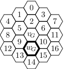
alphaValues is a Dictionary data type in which each -variable, represented as a string, is associated with its value (a rational number). The variable name consists of a bit-string that encodes the -region associated with the variable in the following way. Each vertex of the region is given a label from the set according to Figure 12. For , the th bit (starting from the left) of the variable name is 1 if and only if the vertex labelled is in the region associated with the variable. In other words, the bit-string is a characteristic vector of the set of vertices of .
Comment 3
The program goes through all -variables, confirming that their values are in the range .
Comment 4
Defines .
Comment 5
The 39 -values are set. mu[i] holds the value .
Comment 6
The array G represents a subregion of . Each vertex of the region is given a label from the set according to Figure 12. For , if G[i] is 1 then the vertex labelled is in the region represented by G. If G[i] is 0 then the vertex is not in the region.

Starting with G containing all zeros, for each round in the while-loop, the array G is updated like a 17-digit binary counter. Thus, when G[17] is set to 1, all combinations of the first 17 bits have been considered, and the program breaks out from the while-loop (which ends the program). A configuration of the array G corresponds to a region in the statement of Lemma 7.
Comment 7
If all five neighbours of (labels 9, 10, 13, 14, 15) are in G, proceed with the next region.
Comment 8
Starting with an empty list muList, the program goes through all and checks whether is a subregion of G. If so, is added to muList. The program also considers the mirrored version of . Figure 15 illustrates the overlaps of the -regions and .
Comment 9
The variable minMu is set to the such that is minimised over the s in muList. Note that is the largest of all -values.
Comment 10
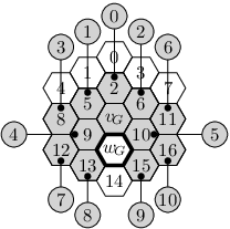
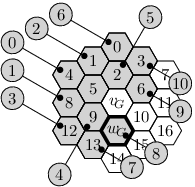
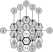
The regions alphaA through alphaF are subregions of , defined according the overlaps of and in Figures 13a–13f, respectively. This corresponds to the overlaps in Figure 7. The strings alphaAstring through alphaFstring are the names of the -variables associated with each of the seven subregions of .
Comment 11
The program now verifies Equation (2) in the statement of Lemma 7. The variables LHS and RHS correspond to the left hand side and right hand side, respectively, of the equation. First, for each neighbour of that is in the region (G in the code), add the corresponding -value to LHS, and then finally multiply the sum with (which is mu[minMu] in the code). The value of RHS is the value of alphaAstring times .
Summary
When running the program lemma7.py, we note that no “complaints” are outputted, which implies that Lemma 7 is successfully proved.
A.2 Computing the -values
The programs that compute the values are called mu1.c, mu2.c, and so on, up to mu39.c, respectively. They are written in C. Using Python for this task would be way too slow. All 39 programs include the file mutop.c, which contains code that runs at the very beginning of every mu-file. The file mutop.c contains macro definition of various for-loops and if-statements, and also defines a large set of variables. The purpose of this file is to keep the code of the mu-files short and concise, with focus on the actual region and its vertices without cluttered C-syntax. This is important when checking the correctness of the programs.
In order to describe the programs, we use the file mu10.c as an example and go through its code in detail. The structure of the other programs is the same.
We break the code into blocks and describe each block separately.
The file mu10.c
1 /* 2 mu.0.1.2.3.5.6.7.8 3 31648 4 123341 5 Output from the program: 6 63296 7 246682 8 13h34m (exact)
The lines above are comments in the code. We focus on the relevant lines. Recall that . Line 3 is the numerator and Line 4 is the denominator. The output from the program is not the -value in its shortest form. The output is specified by Lines 6 and 7 as the numerator and denominator, respectively. Line 8 gives the time it took to run the program in hours and minutes. Obviously this varies from machine to machine, but it gives a rough estimate. The word “exact” here is referring to the computations as being exact and not randomised (remains from the past).
The next few lines of the code are given in Figure 14. They illustrate a labelling of the vertices of the region and a labelling of the boundary vertices. To make the description more comprehensible, we also show a drawing of the region on top of the code.
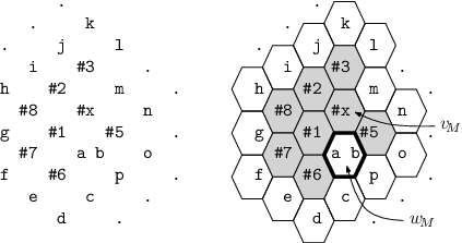
In the code, the numbering of the vertices of the region will be used in the variable names relating to them. The variables represent the boundary vertices. They define the colours of the boundary edges. For this reason, a and b are two variables of the same vertex ; a is the colour of the boundary edge incident to #1 and #6, and b is the colour of the boundary edge incident to #5.
9 #include "mutop.c" 10 BEGIN; 11 AB C D_ E F G H I J K L_ M N O_ P_ 12 {
Line 9 includes the file mutop.c, which defines macros and initiates the code with the main()-body, in which relevant variables are declared. We use upper-case letters for macros and constants, and lower-case letters for variables.
Line 10 records the start time of the execution. This line is irrelevant for the actual computation of .
Every letter of Line 11 corresponds to a for-loop. That is, Line 11 defines a list of nested for-loop, each of which corresponds to the colour of a boundary edge. For example, AB loops through the two configurations and , which are two choices of a and b we need to consider.
The macro C loops trough possible colours of c, which are 0, 1, 2 and 3. As described earlier, we do not need to consider other colours than those on c. The macro definitions take care of the bounds on possible values of the variables. For this particular macro C, the following lines from mutop.c are relevant.
#define FOR_START(c, uc)  for(c = QL, uc = 3; c <= uc; c++)
#define C                 FOR_START(c, uc)
QL is 0 and is the smallest colour and uc is the upper bound on colours of c, which is always 3. As we will see below, the variables representing such upper bounds vary as we progress though the for-loops.
Next on Line 11 is the macro D_. The underscore character specifies that d it is tied closely to the previous colour c in the sense that the ordering of c and d does not matter when computing the -value. This symmetry was explained in Section 8.1. The for-loop associated with d ensures that d is never smaller than c. Here are the relevant lines from mutop.c.
#define FOR_NEXT_(d, ud, c, uc)
        for(d = c,  ud = min(max(uc, c+1), 9); d <= ud; d++)

#define D_  FOR_NEXT_(d, ud, c, uc)
We see above that the upper bound ud on values of d depends on the current value of c; only if c has reached the value 3, we allow d to take on the next value 3+1=4. Otherwise the maximum value of d is set by the upper bound on c, which is uc (which actually is 3).
The remaining part of Line 11 defines the other for-loops associated with the other boundary vertices. Line 12 specifies the opening of the body of the innermost for-loop.
13 FOR_VERTEX(x) 14 { 15 INITX1(m);
The variable x represents the colour of the vertex . Line 13 is a for-loop that takes the x through the values . Recall from Section 8.1 that for , is the number of proper 9-colourings of the region that agree with the colouring of the boundary and assign the colour to . The code in the body of the for-loop of Line 13 computes . The values are stored in the array vx, where vx[x] is .
Since we do not need the value of when computing , we skip . The macro INITX1 on Line 15 skips to next value of x if , otherwise it sets vx[x] to 0. Further, it tests if the value of x is the same as the value of m (the boundary vertex adjacent to ). If this is the case, we will have a colouring that does not agree with the boundary and we can skip immediately to the next value of x.
The number 1 in the macro name INITX1 refers to the fact that one vertex has to be checked against x, in this case m. The macro INITX2, which is used for other -regions, takes two arguments, and so on. Many macro names contain a number. The number is referring to the number of relevant arguments that the macro takes.
16 FOR_VERTEX(m1) 17 { 18 SKIP2(m1, x, a);
The variable m1 is the colour of the vertex labelled #1 in Figure 14. The for-loop on Line 16 takes m1 from 1 to 9. In order to avoid non-proper colourings or colourings that do not agree with the boundary, we have to skip values of m1 for which or . This test is done with the macro on Line 18.
Unlike vertex #1, we do not use for-loops for the other vertices #2, #3, #5, #6, #7 and #8. The running time would be too long with that many nested for-loops. Instead we resort to a dynamic programming approach. Similarly to the array vx, we use one array per vertex. The arrays are called v2, v3, v5, v6, v7 and v8, respectively. The ordering of the arrays by which we fill in their values is first v6, then v7, v8, v2, v3, and lastly v5. For , the value of, for instance , is the number of proper colourings of the subregion consisting of the vertices up to and including #2, which are #6, #7, and #8, subject to the boundary and the value of x and m1, and such that vertex #2 has colour .
19 ONES (v6); ZERO5 (v6, m1, a, c, d, e); 20 NEXT (v7, v6); ZERO4 (v7, m1, e, f, g); 21 NEXT (v8, v7); ZERO4 (v8, i, m1, g, h); 22 NEXT (v2, v8); ZERO4 (v2, j, x, m1, i); 23 NEXT (v3, v2); ZERO5 (v3, k, l, m, x, j); 24 GAP (v5, v3); ZERO6 (v5, m, n, o, p, b, x);
Let us start with Line 19. The array v6 is first initiated with 1 at every position. The following macro, ZERO5, sets the positions m1, a, c, d and e of v6 to 0. The reason is that vertex #6 cannot have the colour specified by these variables as this would violate the property of the colouring being proper or in agreement with the boundary. For the valid colours of #6, there is only one colouring, since the subregion consists only of the single vertex #6.
On Line 20, NEXT(v7, v6) fills in the values of the array v7, subject to the colour of v6. For ,
| (9) |
The number of colourings of the subregion such that #7 has colour is obtained by summing the colourings of the subregion , excluding the case when #6 has colour as this would not make the colouring proper. Hence the subtraction of v6[j]. In the code of mutop.c, there is a macro called SUM which calculates the sum. It is called from the ZERO-macros to prepare for the subsequent NEXT-macro. Once the NEXT-macro has been executed, we must make sure that colourings not in agreement with the boundary are excluded. For instance, v7[3] must be 0 if the boundary edge specified by g is 3. The macro ZERO4 on Line 20 takes care of this, setting appropriate elements of v7 to zero according to the indices specified by m1, e, f and g.
The program proceeds with the remaining vertices on Lines 21–24. The difference between the macro NEXT and the macro GAP on Line 24 is that the two vertices referred to in the argument of GAP, here #3 and #5, are not adjacent. In this case, the array v5 is filled in according to Equation (9) but without the subtraction.
25 UPDATEX(v5); 26 } 27 } 28 UPDATEMU; 29 } 30 END; 31 return(0); 32 }
After Line 24, the sum is the number of proper colourings of the whole region such that vertex has colour x and vertex #1 has colour m1. The macro UPDATEX(v5) on Line 25, inside the body of the for-loop of m1, computes the sum and adds it to vx[x]. Thus, over all values of m1, the final value of vx[x] is computed. The closing bracket on Line 27 indicates the end of the body of the for-loop of x. When Line 28 is reached, the vector vx contains every value we need.
UPDATEMU on Line 28 computes the -value
and compares it to the maximum of all -values computed so far. The maximum value of is stored with the two variables maxnum and maxden, where maxnum is the numerator and maxden is the denominator. Both variables are integers of the data type double to allow enough digits. The comparison of with is performed by multiplying with the denominators to ensure integer arithmetic. If the newly computed value of exceeds the previously largest -value, maxnum and maxden are updated accordingly.
On Line 29, the program proceeds to the next boundary and computes the -value over again.
Finally, on Line 30, after all boundaries have been considered, the largest -value is outputted as well as how long the program has been running.
Part 1 of 5

Part 2 of 5

Part 3 of 5
Part 4 of 5
Part 5 of 5