Evolutionary dynamics of the most populated genotype on rugged fitness landscapes
Abstract
We consider an asexual population evolving on rugged fitness landscapes which are defined on the multi-dimensional genotypic space and have many local optima. We track the most populated genotype as it changes when the population jumps from a fitness peak to a better one during the process of adaptation. This is done using the dynamics of the shell model which is a simplified version of the quasispecies model for infinite populations and standard Wright-Fisher dynamics for large finite populations. We show that the population fraction of a genotype obtained within the quasispecies model and the shell model match for fit genotypes and at short times, but the dynamics of the two models are identical for questions related to the most populated genotype. We calculate exactly several properties of the jumps in infinite populations some of which were obtained numerically in previous works. We also present our preliminary simulation results for finite populations. In particular, we measure the jump distribution in time and find that it decays as as in the quasispecies problem.
I Introduction
The question of mode in evolution, especially in the context of speciation has engaged the attention of many evolutionists for over a century and continues to do so Fitch and Ayala 1994. The issue is whether evolution occurs by smooth gradual changes (gradualism) as put forwarded by Darwin, or sudden large jumps (punctuationism) Mayr 1963; Eldredge and Gould 1972. Some examinations of fossil record indicate that new species can arise by either mode, or even by a combination of the two Benton and Pearson 2001. However, a complete and unambiguous answer is hard to obtain at the level of macroevolution due to the incompleteness and irreproducibility of the fossil data. In the last decade or so, researchers have become interested in carrying out long-term evolution experiments in the laboratory Elena and Lenski 2003. Typically one starts with a microbial population maladapted to a given environment such as a colony of starving bacteria, and track its evolutionary trajectories for thousands of generations as it undergoes adaptive changes. The results of such experiments have been found to be consistent with both modes of evolution. For instance, large populations of RNA virus starting from a low fitness ancestor have been seen to gain fitness in a continuous manner Novella et al. 1995. On the other hand, the fitness of bacteria E. Coli Lenski and Travisano 1994; Imhof and Schlotterer 2001 and RNA virus Burch and Chao 1999 show a punctuated pattern of evolution.
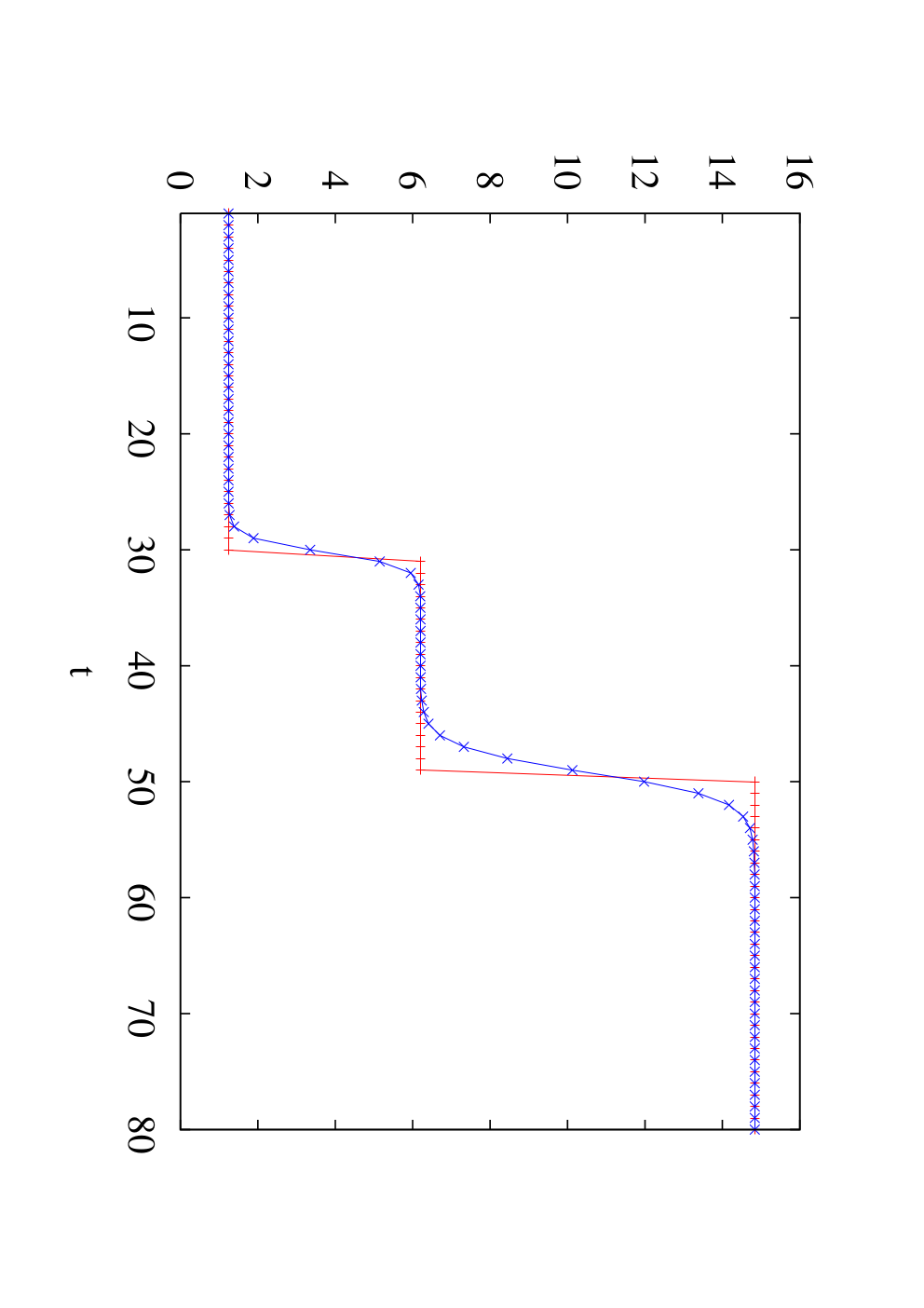
Theoretically, these results are understood using the concept of fitness landscape Wright 1932; Stadler 2002; Gavrilets 2004 defined as a map from the genotypic space into the real numbers. If the fitness landscape is smooth and single-peaked, starting from a low fitness state the population fitness increases gradually until it has reached the peak value Tsimring et al. 1996. The dynamics are different for a population moving on a rugged fitness landscape with multiple peaks Kauffman 1993. In this case, the population fitness increases smoothly until the population encounters a local fitness peak where it gets trapped as a better peak is separated by a fitness valley. The population thus enters the stasis phase and waits until a favorable mutation allows it to shift to a better peak where it can again get localised and so on. Thus, the dynamics alternate between periods of stasis and rapid changes in fitness when the population jumps from a peak to an even better one. An example of this behavior is shown in Fig. 1.
That the fitness landscape underlying the evolutionary process is multi-peaked is supported by several experiments Korona et al. 1994; Lenski and Travisano 1994; Burch and Chao 1999; Burch and Chao 2000; Poelwijk et al. 2007; Fernandez et al. 2007. Besides, these landscapes include biologically important and ubiquitous epistatic interactions Whitlock et al. 1995 as the contribution of individual genes to the fitness of the genotype is not independent Kauffman 1993. The class of landscapes considered in this work are maximally rugged and characterised by strong selection Jain and Krug 2007a. In statistical physics, such rugged landscapes with a large number of local optima have appeared in the context of spin glass theory. Examples include random energy model Derrida 1981 and Sherrington-Kirkpatrick model Sherrington and Kirkpatrick 1975 where the energy of a spin configuration plays the role of genotypic fitness and the metastability in the spin glass dynamics can be viewed as punctuated equilibrium Sibani and Dall 2003.
We are interested in the statistics of jumps which occur when the population fitness changes rapidly. As illustrated in Fig. 1, an unambiguous way of defining a jump at time is the change in the fitness or identity of the most populated genotype at . The problem of such leadership changes arises in several other contexts such as change in the position of the optimal end point of directed polymer Krug and Halpin-Healy 1993, highest degree node in a growing network Krapivsky and Redner 2002; Ben-Naim and Krapivsky 2004, and velocity and position of the front particle in a single-file system Bena and Majumdar 2007; Sabhapandit 2007. In the following sections, before analysing the realistic case of finite populations, we will study the infinite population limit in detail. We consider the dynamics of Eigen’s model Eigen 1971 that describes the population dynamics of self-replicating molecules which at low mutation rates and large times form a dynamic and heterogeneous quasispecies consisting of fittest genotype and its closely related mutants. The existence of such an error threshold is a generic result seen in both simple and complex fitness landscapes, and has been reviewed in Jain and Krug 2007b (for recent related works, see Nilsson and Snoad 2000; Kamp and Bornholdt 2002; Saakian et al. 2006; Park and Deem 2007). The focus of this article is however the dynamics of the quasispecies model. We show that the population fraction at a genotype obtained within a simplified shell model Krug and Karl 2003 (also see Zhang 1997) of quasispecies dynamics is good only for highly fit sequences and at short times. However, the behavior of the most populated genotype is captured correctly by the shell model. We calculate exactly some properties of the jumps (as defined above) within the shell model which were obtained numerically in previous works Krug and Karl 2003; Krug and Jain 2005; Jain and Krug 2005. Specifically, we show that the jump distribution decays as in time and as a function of the distance from the starting genotype for a class of fitness landscapes.
The basic difference between a finite and infinite population is that while the former has a finite mutational spread in the genotypic space, all the mutants are available at all times in the quasispecies limit. Due to this reason, at large times, a finite population gets trapped at a local fitness peak and the jump probability is governed by the rate of stochastic tunneling Iwasa et al. 2004; Weinreich and Chao 2005 which allows the population to cross the fitness valley via few low fitness mutants. In the quasispecies model on the other hand, the reproduction or selection plays the more important role than the production of mutants and a jump occurs when the population at a fit genotype overtakes the less fitter one. Although the underlying physical processes responsible for a jump are different for finite and infinite populations, we find that the jump distribution is robust in that it decays as in both the cases.
The plan of the paper is as follows. In the next section, we define a class of mutation-selection models. Section III discusses the dynamics of quasispecies model and shell model. We calculate exactly the statistics of jumps within the shell model in Section IV. These results for infinite population limit are compared with those obtained in simulations of finite population in Section V. Finally, we conclude with a summary of our results.
II Models
We consider a haploid, asexual population of size each of whose constituents carry a string of length where can assume values. The string can represent a genetic sequence (), protein () or a sequence of loci with alleles Jain and Krug 2007b. For simplicity, we will deal with binary sequences for which and or . The environment of the population is represented by a fitness landscape which is obtained by associating a non-negative real number to each sequence. In this article, we consider fitness to be a random variable chosen independently from a common distribution . This generates a maximally rugged fitness landscape with an exponentially large number (in ) of local maxima Flyvbjerg and Lautrup 1992; Kauffman 1993 and strong interactions amongst the loci Jain and Krug 2007a. The population evolves on this fitness landscape in discrete time via selection and mutation, and we ignore other factors responsible for genetic mixing such as recombination. Our model is thus applicable to microorganisms like E. Coli and Hepatitis C virus which have zero or very low recombination rate Posada et al. 2002.
Consider a population well adapted to a given environment localised around a peak of the fitness landscape. A change in the environment brings about a change in the fitness landscape, and the population will typically find itself in a fitness valley. We consider the adaptation process of the population starting from such an initial condition. The population fraction of sequence at time is iterated using Wright-Fisher dynamics defined as follows. In each generation, an offspring selects a parent with probability where is the fitness of the parent with sequence and is the average fitness of the population. Then the probability that parent has offspring in one generation is given as
This implies that the average number of offspring produced equals and hence the fitness has the physical meaning that it is proportional to the number of descendants produced per generation. Further, as the relative variance in the offspring number decays as , it follows that the offspring number fluctuates from one generation to another for finite population but one can ignore these fluctuations arising due to random sampling for . After the reproduction process, point mutations are introduced independently at each locus of the sequence with probability per generation. Thus, a sequence is obtained via mutations with the probability
| (1) |
where the Hamming distance is the number of point mutations in which the sequences and differ.
Since the selection process is not stochastic for infinite populations, the population frequency also does not fluctuate and one can work with the average frequency where the averaging is over all realizations of the sampling process. This leads to a deterministic nonlinear equation for the fraction Jain and Krug 2007a,
| (2) |
where the denominator is the normalization constant.
III Dynamics of Quasispecies and shell model
The focus of this section is the quasispecies model and the related shell model. In the following, we will mainly work with the unnormalised population defined as Jain and Krug 2007b
| (3) |
in terms of which the nonlinear evolution (2) reduces to the following linear iteration
| (4) |
Since at the start of the adaptation process the population finds itself at a low fitness genotype, we start with the initial condition where is a randomly chosen sequence. For small mutation probability () as seen in various asexual microbes Drake et al. 1998; Jain and Krug 2007b, after one iteration we have
| (5) |
Thus each sequence gets populated in one generation with a fraction which is same for all the sequences in a shell of constant Hamming distance from the initial sequence Krug and Karl 2003. Numerical simulations of Krug and Karl 2003 showed that dynamical properties involving the most populated genotype such as the distribution of evolution times and number of jumps are very well described by a simplified model which ignores mutations for further evolution and allows the population at each sequence to grow with its own fitness. Thus within the shell model, the population for .
Here we provide an analytical understanding of the quasispecies model leading to the shell model. We will find that the expression for in shell model is a good approximation for sequences with high fitness and at short times. For , consider (4) for a sequence in the shell centred about and at a Hamming distance from the center. The sum on the right hand side of (4) has three kind of terms: (i) sequence does not mutate (i.e. in the sum) so that its contribution , (ii) a mutation occurs in where is the set of ’s lying inside shell that satisfy resulting in dependence and (iii) a mutation occurs either in the sequences in the inner shells that do not belong to set or, in the sequences in and outside shell giving a term of order and higher. In order to obtain to order , we can neglect the last contribution and iterate the population according to
| (6) |
The above equation is still coupled but one can make further simplifications by proceeding as follows. Let us first consider the zeroth shell i.e. sequence for which we immediately have
| (7) |
For the sequences in the first shell for which , the sequence is the only member of set and we have
| (8) |
Defining , we obtain a simple difference equation for which can be iterated to give
If , the population grows exponentially fast with a rate equal to its own (log) fitness whereas in the opposite case, this growth rate is that of the initial sequence. For the sequences in the first shell, one therefore obtains
| (9) |
For the succeeding shells, one can work out the population in a manner similar to above and find that if the fitness is larger than that of all the sequences in set . Such a random variable whose value is larger than all the ones preceding it defines a record Jain and Krug 2005; Krug and Jain 2005. If the fitness is not a record, then the growth rate is given by the largest (log) fitness of sequences in set i.e. the last record value.

A comparison of the results obtained using above approximations with the exact iteration of (4) is shown in Fig. 2 for the initial sequence and some representative sequences in the first shell. The disagreement at large times occurs because (7) and (9) are obtained to leading order in and after some time as the population at the outer shells grow, the next order terms in start contributing. For the zeroth shell, this happens at time when the next order terms due to sequences in shell one become as large as the lowest order term given by (7) i.e. where is the largest fitness in the shell . Plugging in the fitness values of relevant sequences in this expression for the fitness landscape in Fig. 2, we obtain in good agreement with the exact iteration. After time , the population at grows with the fitness until the shell starts contributing. This argument can be generalised to higher shells straightforwardly. For instance, the correction to (9) is of order which arises either due to the sequences in the first shell but two mutations away from or the sequences in the second shell that are one mutational distance away. The larger of the two contributions can be then used to estimate the time at which the growth rate changes. This process of slope changes of logarithmic population goes on until the globally fittest sequence becomes most populated after which the population .
In Fig. 2, the initial sequence with rank remains most populated until time steps after which the sequence ranked overtakes it and becomes the next leader. We are interested in such leadership changes and will use the shell model for this purpose as it correctly captures the dynamical behavior of the most populated genotype. Recall that in the shell model, the population at each sequence grows with its own intrinsic fitness for all . This population dynamics are different from quasispecies in which the population of a sequence whose fitness is not a record grows with the fitness of the last record (in inner shells) at short times and the growth rate of the sequences change as the leading genotype changes in course of time. However, since the population at such sequences is always at least order smaller than that at the leading genotype, the dynamics of the most populated sequence are not affected if the population at such sequences is also allowed to grow with their respective fitness.

After these considerations, we arrive at the shell model in which the logarithmic population obeys the following linear time evolution
| (10) |
Calling and rescaling time by , we have
| (11) |
where we have absorbed the extraneous factors in the definition of logarithmic population . Since the population at is same for sequences at constant , only the sequence with the largest fitness in shell need to be considered Krug and Karl 2003. If the logarithmic fitness is distributed according to the distribution , then the largest fitness in shell which is the maximum of variables is distributed independently but non-identically with distribution
| (12) |
where is the lower support of the distribution .
IV Statistics of jumps in shell model
In the following, we will consider the shell model dynamics defined as
| (13) |
where and respectively are the fitness and population of the sequence with the largest fitness in shell . Figure 3 shows the population as a function of time for as the global maximum of the fitness landscape in Fig. 2 lies at a Hamming distance from the initial sequence. Since a line intersects at a time
| (14) |
and as , the population of the sequence in shell is overtaken by the one in shell . However to become a most populated genotype, it is not sufficient to have a record fitness. As Fig. 3 shows although , the population overtakes later than losing the evolutionary race. Thus, only those set of sequences become leader that manage to overtake the current leader in the least time amongst all contenders. Finally, the globally fittest sequence catches up with and the population localises at the global peak Krug and Karl 2003; Jain and Krug 2005.
The shell model defined by (13) describes a population growing linearly in time with a slope equal to the fitness chosen from the distribution . A simpler version of this model in which the fitness are assumed to be independent and identically distributed (i.i.d.) variables with distribution has also been considered Krug and Karl 2003; Jain and Krug 2005. Several properties of this model have been recently calculated via a mapping to a first-passage problem Sire et al. 2006 and considering it as a system of hard-core particles undergoing elastic collisions Bena and Majumdar 2007. In particular, it has been shown that the average number of jumps grows as where the prefactor and depends on the choice of . In both of these approaches, the initial condition (the intercept) of is not fixed and is a uniformly distributed random number on the real line. In this article, we present a way to calculate average number of changes in which respects the discreteness of the underlying genotypic space. We will perform the calculations for the shell model for which the fitness is non-identically distributed, although our method is readily applicable to the i.i.d. model also. However, we mention that the prefactor calculated using our method turns out to be the same as in the analysis of Sire et al. 2006; Bena and Majumdar 2007.
IV.1 General formulae
To calculate the statistics of jumps, we need two basic distributions: (i) the probability that the most populated sequence in shell with fitness is the leader at time and (ii) the probability with which this sequence is overtaken by the most populated sequence in shell between time and . The distribution requires that the population , which implies that the fitness . Since the fitnesses of the most populated sequence in each shell are independent random variables, we have
| (15) |
To find , we need to determine the fitness of the most populated sequence in shell which can contribute to the overtaking event. Let us denote the location of the leader at time by ,
Then the sequence in shell can overtake the th one at if the fitness . Similarly, the sequence in the th shell can be overtaken at , if
Thus the probability that a sequence in shell is overtaken by a sequence in shell between time and is given by
| (16) |
Finally using the distributions defined in (15) and (16), we can write the probability that the most populated sequence in shell overtakes the one in shell at time as
| (17) |
where is the upper support of the distribution .
Depending on the quantity of interest, one can either integrate over time or sum over a space variable in . Often the experimental data such as a morphological feature Benton and Pearson 2001 or average fitness Elena and Lenski 2003 are plotted as a function of time and can be used to find the number of jumps in time. Therefore it is useful to consider the distribution of a jump to occur at time which can be found by summing over and ,
| (18) |
The relationship between the overtaken and the overtaking sequence can be deduced by computing the jump distribution that the most populated sequence in shell is a jump given by
| (19) |
The average number of jumps can be obtained by either integrating over time or summing over .
In the previous works on shell model Krug and Karl 2003; Jain and Krug 2005; Krug and Jain 2005, several properties of the jumps have been studied numerically when the fitness is distributed according to an exponential or Gaussian distribution. In the following subsections, we will use the expressions derived above for the exponential case which lends itself to a detailed analysis and then give some results for fitness distributions decaying faster than an exponential.
IV.2 Exponentially distributed fitness
We consider for which the largest fitness in shell is distributed according to
| (20) |
Using this in (15), we obtain the distribution that the leader with fitness is in shell ,
| (21) | |||||
where the last expression is obtained by exponentiating the product and keeping only the leading order terms in the expansion. Similarly, the overtaking rate (16) can be written as
| (22) | |||||
Then the probability that the population in the th shell exceeds the population in the th shell at time is given by
| (23) |
Neglecting the first term in the exponent of the exponential in the integrand and carrying out the integral for large , we finally obtain
| (24) |


We will now use this expression to calculate jump statistics.
Temporal behavior-. Let us first consider the distribution of a jump to occur in the th shell at time . Summing over , we obtain Gradshteyn and Ryzhik 1980
| (25) |
where is the gamma function and is the hypergeometric function. We point out that the distribution gives the probability that is overtaken at and hence differs from the distribution that is the largest at time considered in Jain and Krug 2005. The function is plotted as a function of time for various values of in Fig. 4. To gain some insight into the behavior of this distribution, we calculate the above sum using saddle point approximation. Using the Stirling’s formula for binomial coefficient
| (26) |
in (25) for and approximating the sum over by an integral, we have
where we have estimated the integral using the saddle point method. In the above expression, , is the second derivative of evaluated at the minimum of the function and the deviation . Explicitly,
Approximating the factor in (25) also by a Gaussian in a manner similar to above, we finally have
| (27) |
Using this expression, it is easy to obtain the typical shell location of the sequence overtaken at time by integrating over . Since is normalised to , we find that given an overtaking event occurs at , the average location of the overtaken sequence scales as with a standard deviation of order about it. This length scale can also be expressed in terms of time for fixed as the distribution is maximised at or . Thus for large , the time at which is most probable is given by
| (28) |
This means that a sequence with is most likely to be overtaken in a time of order unity. This fact is also expressed in Fig. 4 which shows the distribution at fixed as a function of time. The time scale can be understood by a simple argument which estimates the intersection time given by (10). This argument is analogous to that used in Krug and Karl 2003; Jain and Krug 2005; Jain and Krug 2007a where the fitness difference in the denominator of (10) is given by the typical value of the fitness gap which probes the rare events. As we are interested in the most likely events, the denominator is approximated by the difference in the average value of the largest fitness in shell and . From (20), we see that the average largest fitness goes as . Since typically the most populated sequence in shell is overtaken by a sequence located distance away Jain and Krug 2005 (also see below), the numerator of (10) scales as and the denominator on using the Stirling’s formula turns out to be thus leading to (28).
Although the most probable value of the overtaking time is of order one, the average overtaking time is infinite due to the fat tail of the distribution . For , we can approximate by and using the asymptotic expansion of error function for large argument Arfken 1985,
| (29) |
we obtain
| (30) |
Due to the behavior at large times shown in the inset of Fig. 4, the mean time diverges for any and (see below). The tail of this distribution is exponentially suppressed in for finite but goes as for close to . The late time behavior above is also obtainable from (10) by a simple change of variables Krug and Karl 2003; Jain and Krug 2005.
After performing the integral over in (27), we obtain
| (31) |
Integrating over time from to infinity, we find that the average number of jumps grows as .
Spatial behavior-. One can also find the probability that the most populated sequence in the th shell is a jump. As we are not interested in temporal distribution, the integral over time in (24) can be carried out to give the probability that the sequence in shell is overtaken by that in shell ,
| (32) |
This distribution is shown for some representative parameters in Fig. 4. Approximating the integrand in the above equation by a Gaussian centred about inverse time and carrying out the integral, we obtain
| (33) |
The argument of the error function changes sign when . For , the argument is negative and of order . Using (29), we find that the last factor in (33) is exponentially small in for . Thus the probability that the overtaking sequence lies beyond the shell is negligible. This is understandable as the globally fittest sequence is typically located in the shell Jain and Krug 2005. For , the error function in (33) can be approximated by unity, and the probability distribution can be further simplified to give
| (34) |
where we have used the Gaussian approximation for the binomial coefficients. This form of the distribution implies that the overtaking sequence is located within distance of the overtaken sequence . Thus the typical spacing between successive jumps for large is roughly constant and goes as as seen in the numerical simulations of Jain and Krug 2005. The jump distribution for a jump to occur in shell is obtained by integrating over and we have
| (35) |
where is the Heaviside step function. Thus the distribution decays as for in accordance with the numerical results of Jain and Krug 2005; Krug and Jain 2005. Integrating the preceding equation over , we find that the average number of jumps are given as in agreement with the previous calculation.
IV.3 Gumbel-distributed shell fitness
We now consider , for which the distribution of the largest of random variables for large has the Gumbel distribution as the limiting form David 1970,
| (36) |
where
| (37) |
We will show that the tail of the distribution decays as and the average number of jumps scales as for any .
The large time behavior of can be found by taking limit in (15) and (16) except for the factor in rate . We thus have
| (38) |
after using the approximations similar to those used in arriving at (24). The sum under the integral sign can be computed by saddle point approximation so that the integral (up to scale factors) is writeable as
where we have neglected the logarithm of in and for large . Since we are interested in large times when , to leading order in , we find thus simplifying the expression for to yield
| (39) | |||||
where the last expression is obtained by estimating the sum over using Gaussian approximation. For small () and , this expression reduces to (30) for exponential distribution. For , the dependence in the preceding equation consists of two factors, the first one arising because the typical separation for large Krug and Karl 2003; Jain and Krug 2005 and the last factor is due to , left after scaling the fitness in (38) by .
In order to find the average number of jumps, we first need to calculate for arbitrary . As argued in the last subsection, is given as the derivative (with respect to ) of the average shell fitness. From the scaling form (36), we see that the average shell fitness is proportional to . For of order , its derivative grows as , . Then integrating over and , we find that the average number of jumps scale as for all . This result is also consistent with the simulations for the Gaussian distribution in Krug and Jain 2005.
V Jump distribution for finite populations
We will now consider the dynamics of a population of individuals evolving according to the Wright-Fisher dynamics described in Section II. Unlike the infinite population, a population of size initially localised at sequence can spread up to a finite distance. This is since the typical fraction of the population at a sequence in one generation is given as but as this fraction is bounded below by , it follows that the mutational spread for a finite population. Thus while all the mutants are available in one generation for quasispecies (see (5)), only a finite number is present at any time in real populations. If a fitter sequence is available within this effective distance, the population behaves like a quasispecies and evolves deterministically. This is possible for and at short times Jain and Krug 2007a. However at long times, any finite population can get trapped at a local peak if a fitter sequence lies farther out than . In such an event, the population escapes the local peak via the process of stochastic tunneling which takes a time given by Iwasa et al. 2004; Weinreich and Chao 2005
| (40) |
for where refers to the fitness of the initial and final local peak separated by two mutations. During this time, most of the population stays at the local peak with fitness but a few less-fit mutants are produced by single mutations. When some of these mutants further acquire a favorable mutation, then the whole population quickly jumps to the next local peak with higher fitness . The physical process involved when a jump occurs in a finite population is thus different from that in the quasispecies case. In the latter case, each local peak is already populated albeit with a small frequency and a jump occurs when the population at a fitter sequence overtakes the current leader.
We are interested in the jump distribution of large finite populations with close to one. At large times when the tunneling drives the dynamics, we expect the density of jumps at to scale as
| (41) |
where is the typical fitness of the local peak visited at separated by a better peak with fitness difference . We expect to decrease and to increase with time as higher peaks are explored. However in the absence of an argument for these time dependences, we present our preliminary numerical results here. In the shell model, one does not have to deal with the whole genotypic space consisting of sites and it suffices to work with the shells thus reducing the computational effort enormously Krug and Karl 2003. However such a rotational symmetry is not present for the finite population problem so we are able to handle only small values of . Our numerical results for large finite populations and small are shown in Fig. 5 for exponentially distributed log fitness or as in the last sections. The data in Fig. 5 are averaged over several histories as the evolutionary trajectories are not deterministic for finite populations Jain and Krug 2007a. For fixed and , we find that at long times,
| (42) |
which decays the same way as in the quasispecies model,
| (43) |
where we have reinstated the dependence.

VI Conclusions
In this article, we discussed the evolution of asexual population on rugged fitness landscapes with many local optima separated by valleys. We focused on the statistical properties of the most populated genotype which changes as the population locates better peaks in the fitness landscape. These properties were calculated exactly within a shell model which was derived systematically from the Eigen’s quasispecies model for infinite populations. We showed that the expression for the population frequency within shell model approximates the quasispecies solution well for highly fit sequences and at short times only. However, the two models are equivalent as regards the statistics of the most populated genotype. We computed the average number of jumps in the shell model and found that it grows as , being the sequence length, for fitness distributions decaying as exponential or faster. The jump distribution in time was shown to decay as . This dependence is also seen numerically for the finite population but a satisfactory explanation for this case is presently missing. A more detailed analysis of the finite population properties will be taken up in the future.
Acknowledgement: The author thanks J. Krug for useful comments, Israel Science Foundation for financial support and KITP (Santa Barbara) for hospitality where this work was initiated.
References
- Fitch and Ayala (1994) W. Fitch and F. Ayala, Proc. Natl. Acad. Sci. USA 91, 6717 (1994).
- Mayr (1963) E. Mayr, Animal Species and Evolution (Harvard University Press, Cambridge, 1963).
- Eldredge and Gould (1972) N. Eldredge and S. Gould, in Models in Paleobiology, edited by T. Schopf (W.H. Freeman and Co., 1972), pp. 82–115.
- Benton and Pearson (2001) M. Benton and P. Pearson, Trends Ecol. Evol. 16, 405 (2001).
- Elena and Lenski (2003) S. F. Elena and R. E. Lenski, Nat. Rev. Genet. 4, 457 (2003).
- Novella et al. (1995) I. Novella, E. Duarte, S. Elena, A. Moya, E. Domingo, and J. Holland, Proc. Natl. Acad. Sci. USA 92, 5841 (1995).
- Lenski and Travisano (1994) R. E. Lenski and M. Travisano, Proc. Natl. Acad. Sci. USA 91, 6808 (1994).
- Imhof and Schlotterer (2001) M. Imhof and C. Schlotterer, Proc. Natl. Acad. Sci. USA 98, 1113 (2001).
- Burch and Chao (1999) C. L. Burch and L. Chao, Genetics 151, 921 (1999).
- Wright (1932) S. Wright, in Proceedings of the Sixth International Congress of Genetics, edited by D. F. Jones (Menasha, WI: Brooklyn Botanic Garden, 1932), pp. 356–366.
- Stadler (2002) P. Stadler, in Biological evolution and statistical physics, edited by M. Lässig and A. Valleriani (Springer, Berlin, 2002), p. 183.
- Gavrilets (2004) S. Gavrilets, Fitness landscapes and the origin of species (Princeton University Press, 2004).
- Tsimring et al. (1996) L. S. Tsimring, H. Levine, and D. A. Kessler, Phys. Rev. Lett. 76, 4440 (1996).
- Kauffman (1993) S. A. Kauffman, The Origins of Order (Oxford University Press, New York, 1993).
- Korona et al. (1994) R. Korona, C. H. Nakatsu, L. J. Forney, and R. E. Lenski, Proc. Natl. Acad. Sci. USA 91, 9037 (1994).
- Burch and Chao (2000) C. L. Burch and L. Chao, Nature 406, 625 (2000).
- Poelwijk et al. (2007) F. Poelwijk, D. Kivet, D. Weinreich, and S. Tans, Nature 445, 383 (2007).
- Fernandez et al. (2007) G. Fernandez, B. Clotet, and M. Martinez, J. Virol. 81, 2485 (2007).
- Whitlock et al. (1995) M. C. Whitlock, P. C. Phillips, F. B.-G. Moore, and S. J. Tonsor, Annu. Rev. Ecol. Syst. 26, 601 (1995).
- Jain and Krug (2007a) K. Jain and J. Krug, Genetics 175, 1275 (2007a).
- Derrida (1981) B. Derrida, Phys. Rev. B 24, 2613 (1981).
- Sherrington and Kirkpatrick (1975) D. Sherrington and S. Kirkpatrick, Phys. Rev. Lett. 35, 1792 (1975).
- Sibani and Dall (2003) P. Sibani and J. Dall, Europhys. Lett. 64, 8 (2003).
- Krug and Halpin-Healy (1993) J. Krug and T. Halpin-Healy, J. Phys. I France 3, 2179 (1993).
- Krapivsky and Redner (2002) P. Krapivsky and S. Redner, Phys. Rev. Lett. 89, 258703 (2002).
- Ben-Naim and Krapivsky (2004) E. Ben-Naim and P. Krapivsky, Europhys. Lett. 65, 151 (2004).
- Bena and Majumdar (2007) I. Bena and S. Majumdar, Phys. Rev. E 75, 051103 (2007).
- Sabhapandit (2007) S. Sabhapandit, J. Stat. Mech. p. L05002 (2007).
- Eigen (1971) M. Eigen, Naturwissenchaften 58, 465 (1971).
- Jain and Krug (2007b) K. Jain and J. Krug, in Structural approaches to sequence evolution: Molecules, networks and populations, edited by U. Bastolla, M. Porto, H. Roman, and M. Vendruscolo (Springer, Berlin, 2007b), pp. 299–340, eprint arXiv:q-bio.PE/0508008.
- Nilsson and Snoad (2000) M. Nilsson and N. Snoad, Phys. Rev. Lett. 84, 191 (2000).
- Kamp and Bornholdt (2002) C. Kamp and S. Bornholdt, Phys. Rev. Lett. 88, 068104 (2002).
- Saakian et al. (2006) D. Saakian, E. Munoz, C. Hu, and M. Deem, Phys. Rev. E 73, 041913 (2006).
- Park and Deem (2007) J. Park and M. Deem, Phys. Rev. Lett. 98, 058101 (2007).
- Krug and Karl (2003) J. Krug and C. Karl, Physica A 318, 137 (2003).
- Zhang (1997) Y.-C. Zhang, Phys. Rev. E 55, R3817 (1997).
- Krug and Jain (2005) J. Krug and K. Jain, Physica A 358, 1 (2005).
- Jain and Krug (2005) K. Jain and J. Krug, J. Stat. Mech.: Theor. Exp. p. P04008 (2005).
- Iwasa et al. (2004) Y. Iwasa, F. Michor, and M. A. Nowak, Genetics 166, 1571 (2004).
- Weinreich and Chao (2005) D. M. Weinreich and L. Chao, Evolution 59, 1175 (2005).
- Flyvbjerg and Lautrup (1992) H. Flyvbjerg and B. Lautrup, Phys. Rev. A 46, 6714 (1992).
- Posada et al. (2002) D. Posada, K. Crandall, and E. Holmes, Ann. Rev. Genet. 36, 75 (2002).
- Drake et al. (1998) J. Drake, B. Charlesworth, D. Charlesworth, and J. Crow, Genetics 148, 1667 (1998).
- Sire et al. (2006) C. Sire, S. Majumdar, and D. S. Dean, J. Stat. Mech.: Theor. Exp. p. L07001 (2006).
- Gradshteyn and Ryzhik (1980) I. Gradshteyn and I. Ryzhik, Table of Integrals, Series, and Products (Academic Press, New York, 1980).
- Arfken (1985) G. Arfken, Mathematical methods for physicists (Academic Press, New York, 1985).
- David (1970) H. A. David, Order Statistics (Wiley, New York, 1970).