Holographic spectral functions and diffusion constants for fundamental matterPreprint: arXiv:0706.0162 [hep-th]

Robert C. Myers Andrei O. Starinets Affiliation: Perimeter Institute for Theoretical Physics, Waterloo, Ontario N2L 2Y5, Canada Affiliation: Perimeter Institute for Theoretical Physics, Waterloo, Ontario N2L 2Y5, Canada Affiliation: Department of Physics and Astronomy, University of Waterloo, Waterloo, Ontario N2L 3G1, Canada Affiliation: Kavli Institute for Theoretical Physics, University of California, Santa Barbara, CA 93106-4030, USAE-mail: Email: rmyers@perimeterinstitute.ca, starina@perimeterinstitute.ca, rthomson@perimeterinstitute.ca Rowan M. Thomson Affiliation: Perimeter Institute for Theoretical Physics, Waterloo, Ontario N2L 2Y5, Canada Affiliation: Department of Physics and Astronomy, University of Waterloo, Waterloo, Ontario N2L 3G1, Canada

August 11, 2026

Abstract:

The holographic dual of large- $N_{\textrm{\tiny c}}$ super-Yang-Mills coupled to a small number of flavours of fundamental matter, $N_{\textrm{\tiny f}}\ll N_{\textrm{\tiny c}}$ , is described by $N_{\textrm{\tiny f}}$ probe D7-branes in the gravitational background of $N_{\textrm{\tiny c}}$ black D3-branes. This system undergoes a first order phase transition characterised by the ‘melting’ of the mesons. We study the high temperature phase in which the D7-branes extend through the black hole horizon. In this phase, we compute the spectral function for vector, scalar and pseudoscalar modes on the D7-brane probe. We also compute the diffusion constant for the flavour currents.

Keywords:

D-branes, Supersymmetry and Duality, Brane Dynamics in Gauge Theories

1 Introduction

The gauge/gravity duality has created a powerful framework for the study of strongly coupled gauge theories [1, 2, 3, 4]. Thermal properties of such theories are of considerable interest both in their own right and in connection with the experimental program on heavy ion collisions at RHIC and LHC.

In this paper, we study certain aspects of finite-temperature behaviour of strongly coupled ${\cal N}=2$ super-Yang-Mills theory with dynamical quarks in Minkowski space. The holographic description of the theory with gauge group $U(N_{\textrm{\tiny c}})$ and $N_{\textrm{\tiny f}}$ hypermultiplets in the fundamental representation (as well as one adjoint hypermultiplet) is given by the well studied system of D3- and D7-branes. In the limit of large $N_{\textrm{\tiny c}}$ and large ’t Hooft coupling $\lambda=g^{2}_{YM}N_{c}$ with fixed $N_{\textrm{\tiny f}}$ , the theory is described by $N_{\textrm{\tiny f}}$ probe D7-branes in the near-horizon geometry of $N_{\textrm{\tiny c}}$ D3-branes, i.e., AdS ${}_{5}\times S^{5}$ [5]. At finite temperature, the background geometry contains a black hole [6]. Although the ${\cal N}=2$ theory is non-confining and thus no confinement-deconfinement phase transition is expected at finite temperature, the presence of the quark mass scale $M_{q}$ leads to a first order phase transition for fundamental matter [7]. The transition occurs at a temperature $T\sim M_{q}/\sqrt{\lambda}$ and is characterized by the dissociation or ‘melting’ of the mesons, i.e., the quark-antiquark bound states¹¹ 1 Recall that for these supersymmetric field theories, the fundamental matter includes both fermions and scalars, which we will refer to collectively as ‘quarks’..

Our goal is to study thermal dissociation of the bound states as well as the flavour current diffusion by computing spectral functions of mesonic operators in the framework of gauge/gravity duality.

Refer to caption — Figure 1: Various possible D7-brane embeddings in the black D3-brane geometry with temperature increasing from left to right.

The thermal behaviour of the ${\cal N}=2$ gauge theory with fundamental matter has recently been actively studied [8, 9, 7, 10]. The holographic description gives a simple picture of the phase transition. If the D7-branes are sufficiently far from the event horizon of the black hole, they are gravitationally attracted towards the horizon but their tension is sufficient to balance this attractive force. The probe branes then lie entirely outside of the black hole in what were denoted ‘Minkowski’ embeddings in [7, 10] – see fig. 1. As the temperature is raised, both the radial position and the energy density of the event horizon increase. Therefore, above some critical temperature, the gravitational attraction of the black hole overcomes the brane tension and the D7-branes are pulled into the horizon. These configurations where the branes fall through the horizon are referred to as ‘black hole’ embeddings. In between these two branches, there also exists a critical solution which just ‘touches’ the horizon. Thermodynamic considerations show the latter is by-passed by a first order phase transition, in which the probe branes jump discontinuously from a Minkowski to a black hole embedding.

In the dual field theory, this phase transition is exemplified by discontinuities in various physical quantities, e.g., the quark condensate. However, the most striking feature of the transition is found in the spectrum of the mesons. The latter correspond to excitations supported on the probe branes – see, e.g., [11, 12]. In the low-temperature or Minkowski phase, the mesons are stable (to leading order within the approximations above) and the spectrum is discrete with a finite mass gap. In the high-temperature or black hole phase, mesons are all destabilized and rather one finds a continuous and gapless spectrum of excitations²² 2 For a discussion of thermal resonances in the context of holographic models see e.g., [13].. Accordingly, spectral functions of mesonic operators in the low-temperature phase are characterized by $\delta$ -function peaks³³ 3 A derivation of the scalar meson spectral function at $T=0$ appears in appendix B. (with the decay width of these particles and the continuum contribution of multi-particle states both suppressed by factors of $1/N_{\textrm{\tiny c}}$ ), whereas in the high-temperature phase spectral functions are essentially featureless⁴⁴ 4 The temperature-dependent part of the spectral functions exhibits damped oscillations with the period proportional to a Matsubara frequency, see section 2.3 for details. (fig. 2).

More interesting behaviour is observed when the system evolves from the high-temperature phase into the low-temperature phase through the metastable ‘supercooled’ phase. We show that in this case the serene landscape of fig. 2b is distorted by peaks corresponding to quasiparticle excitations, and these excitations are eventually transformed into the stable resonances shown in fig. 2a.

These features of the spectral functions are controlled by the analytic structure of the corresponding retarded correlators in the complex frequency plane. In the high-temperature phase, the poles of the retarded correlators (with the exception of the poles corresponding to hydrodynamic excitations) are located at a finite distance from the real axis thus making the spectral function featureless. As the temperature is lowered with respect to the quark mass scale, the poles move closer to the real axis and the spectral functions exhibit distinct peaks. Holographically, the poles of the retarded correlators correspond to quasinormal modes of the gravitational background [14, 15]. Numerical investigation of the full quasinormal spectrum of the D3-D7 system faces certain technical difficulties. In this paper we focus on computing the spectral functions for which the numerical methods are reliable.

In addition to characterizing quasiparticle excitations of a thermal system, spectral functions also carry information about the medium’s transport properties. Adapting techniques from [16, 17, 18], we compute the quark diffusion constant as a function of the parameter $M_{q}/T$ in the high-temperature phase, and attempt to give a qualitative description of its dependence on the coupling for the full range of temperatures.

Thermal dissociation of mesons as well as transport properties of the quark-gluon plasma can be studied in lattice QCD with the help of indirect methods such as the maximal entropy method [19, 20, 21, 22, 23, 24, 25, 26, 27, 28]. These studies suggest, in particular, that mesons survive as relatively well-defined resonances at temperatures well above $T_{c}$ ( $2-3T_{c}$ ). While the uncertainties of these lattice methods remain large, the holographic approach used in this paper serves as a source of quantitative and often analytically exact results for qualitatively similar finite-temperature models.

An overview of the paper is as follows: in section 2 we review properties of thermal spectral functions in field theory and outline methods of computing spectral functions from dual gravity. These methods are illustrated by a simple example of computing the spectral function and diffusion constant for $R$ currents in ${\cal N}=4$ SYM. For vanishing spatial momentum, the correlator, quasinormal spectrum, and the spectral function can be computed analytically. In section 3 we introduce the D3/D7-brane framework and review the D7-brane embeddings and thermodynamics. In section 4, we turn to the calculation of the spectral function for various mesonic operators in the high temperature phase of the ${\cal N}=2$ gauge theory. We consider a vector operator in section 4.1. In the special case of vanishing quark mass, we determine the spectral function analytically. In general, for arbitrary quark mass, the vector spectral function is computed numerically. In section 4.2, we turn to spectral functions for scalar and pseudoscalar operators, which are again bilinear in the fundamental fields. Section 5 presents three independent computations of the diffusion constant for ‘light’ quarks, using the membrane paradigm method [17], the Green-Kubo formula, and by calculating the lowest quasinormal frequency for the vector field on the D7-brane. Section 6 contains discussion and observations about our results. Some details of our analysis are relegated to appendices: appendix A provides a review of the holographic dictionary relating the D7-brane worldvolume fields to their dual operators in the gauge theory; appendix B contains a derivation of the scalar spectral function at $T=0$ ; appendix C provides a derivation of the high frequency asymptotics for the spectral functions; appendix D gives a partial analysis of the quasinormal modes for the pseudoscalar and scalar excitations; and finally, appendix E extends the computation of the quark diffusion constant, described in section 5.1, to the holographic framework described by a Dq-brane probe in a near-extremal Dp-brane throat.

2 Prelude: spectral functions and holography

In general, finite-temperature correlation functions of conserved charge densities carry information about a medium’s transport properties and quasiparticle excitations. This information is given, roughly, by the poles and the corresponding residues of the correlators, or, equivalently, by their spectral functions. Recently the study of these objects has been used to great effect in a holographic framework to study the thermal properties of various strongly coupled field theories [40]. In a holographic setting, the spectral functions are often easier to compute than the full correlators on the gravity side. According to the holographic dictionary, the poles are determined by the quasinormal spectrum of a dual bulk field fluctuation, whereas the spectral function is given by the imaginary part of the retarded correlator which is independent of the radial coordinate [15, 29]. In this section, we combine the necessary tools for computing the spectral functions from dual gravity and analyzing their properties, and then illustrate this technique using the simple example of strongly coupled ${\cal N}=4$ supersymmetric $SU(N_{\textrm{\tiny c}})$ Yang-Mills (SYM) theory at large $N_{\textrm{\tiny c}}$ . In this case, the $R$ -current spectral function has been analyzed elsewhere [29, 30, 13] but we present a new analytic result (for vanishing spatial momentum).

2.1 Field theory picture

A thermal spectral function of an operator ${\cal O}$ is defined as⁵⁵ 5 Our metric convention is $(-,+,+,+)$ . We assume translation invariance to be an unbroken symmetry of the theory.

{\swabfamily R}(\omega,{\bf q})=\int d^{4}x\;e^{-i\omega t+i{\bf q}{\bf x}}\langle[{\cal O}(t,{\bf x}),{\cal O}(0)]\rangle\,,

(2.1)

where the correlator is computed in thermal equilibrium at a temperature $T$ . The spectral function is proportional to the imaginary part of the retarded correlator,

{\swabfamily R}(\omega,{\bf q})=-2\,{\rm Im}\,G^{R}(\omega,{\bf q})\,,

(2.2)

where

G^{R}(\omega,{\bf q})=-i\!\int\!d^{4}x\,e^{-i\omega t+i{\bf q}{\bf x}}\,\theta(x^{0})\langle[{\cal O}(t,{\bf x}),{\cal O}(0)]\rangle\,.

(2.3)

If ${\cal O}$ is an operator of a density of a conserved charge in a rotation invariant theory, the retarded thermal two-point function is determined by two independent scalar functions. In Fourier space, the correlator can be decomposed into the transverse and longitudinal parts [29]

G^{R}_{\mu\nu}(\omega,q)=P_{\mu\nu}^{T}\,\Pi^{T}(\omega,q)+P_{\mu\nu}^{L}\,\Pi^{L}(\omega,q)\,,

(2.4)

where the index structure is absorbed into two mutually orthogonal projectors $P_{\mu\nu}^{T}$ and $P_{\mu\nu}^{L}$ . Without loss of generality we can take the spatial momentum oriented along the $x^{3}$ direction, so that $k_{\mu}=(-\omega,0,0,q)$ , with $k^{2}=-\omega^{2}+q^{2}$ . Then one has [29]

G^{R}_{x^{1}x^{1}}(k)=G^{R}_{x^{2}x^{2}}(k)=\Pi^{T}(\omega,q)\ .

(2.5)

Other components of the current-current correlator are

	$\displaystyle G^{R}_{tt}(k)=-\frac{q^{2}}{q^{2}-\omega^{2}}\,\Pi^{L}(\omega,q)\ ,$		(2.6)
	$\displaystyle G^{R}_{tx^{3}}(k)=-\frac{\omega q}{q^{2}-\omega^{2}}\,\Pi^{L}(\omega,q)\ ,$		(2.7)
	$\displaystyle G^{R}_{x^{3}x^{3}}(k)=-\frac{\omega^{2}}{q^{2}-\omega^{2}}\,\Pi^{L}(\omega,q)\ .$		(2.8)

In the long-time, long-wavelength limit (i.e., for $\omega/T\ll 1$ , $q/T\ll 1$ ) the functions $\Pi^{T}(\omega,q)$ and $\Pi^{L}(\omega,q)$ have a universal behaviour dictated by hydrodynamics: $\Pi^{T}(\omega,q)$ is nonsingular as a function of the frequency, while $\Pi^{L}(\omega,q)$ has a simple pole at

\omega=-iDq^{2}\,,

(2.9)

where $D$ is the charge diffusion constant.

The rotation invariance implies that in the limit of vanishing spatial momentum at fixed $\omega>0$ the two scalar functions coincide: $\Pi^{T}(\omega,0)=\Pi^{L}(\omega,0)=\Pi(\omega)$ . Correspondingly, at $q=0$ one can define

{\swabfamily R}(\omega)\equiv{\swabfamily R}_{x^{1}x^{1}}(\omega,0)={\swabfamily R}_{x^{2}x^{2}}(\omega,0)={\swabfamily R}_{x^{3}x^{3}}(\omega,0)\,.

(2.10)

The Green-Kubo formula relates the diffusion constant to the zero-frequency limit of the spectral function ${\swabfamily R}(\omega)$ :

D\,\Xi=\lim\limits_{\omega\rightarrow 0}{1\over 2\omega}{\swabfamily R}(\omega)\,.

(2.11)

Here $\Xi$ is the charge susceptibility. The susceptibility is determined by the thermodynamics of the system in a grand canonical ensemble,

\Xi={\partial n(\mu)\over\partial\mu}\,\Biggl|_{\mu=0}\,,

(2.12)

where $n(\mu)$ is the charge density, $\mu$ is the corresponding chemical potential.

In addition to hydrodynamic poles, the retarded correlators may have other singularities located in the lower half-plane of complex frequency. Assuming one of these singularities is a simple pole,

G^{R}\sim\frac{1}{\omega-\Omega(q,\alpha)+i\Gamma(q,\alpha)}\,,

where $\alpha$ represents a set of parameters relevant for a particular theory, for the spectral function one has

{\swabfamily R}(\omega)\sim\frac{\Gamma}{(\omega-\Omega)^{2}+\Gamma^{2}}\,.

Thus in the vicinity of $\omega=\Omega$ , the spectral function has a peak characterized by a width $\sim\Gamma$ and a height (‘lifetime’) $\sim 1/\Gamma$ . The peak has a quasiparticle interpretation if $\Gamma\ll\Omega$ .

The spectral function ${\swabfamily R}(\omega)$ also has a characteristic form in the high frequency limit. This behaviour is determined by the leading short-distance singularity

\lim_{(t^{2}-{\bf x}^{2})\rightarrow 0}\langle{\cal O}(t,{\bf x})\,{\cal O}(0)\rangle=\frac{{\cal A}}{|t^{2}-{\bf x}^{2}|^{\Delta}}+\cdots\,,

(2.13)

where $\Delta$ denotes the dimension of the operator $\cal O$ and $\cal A$ is a dimensionless constant. A Fourier transform then leads to the following contribution to the spectral function

{\swabfamily R}(\omega)\sim{\cal A}\,\omega^{2\Delta-4}\ .

(2.14)

2.2 Gravity picture

In the dual gravity picture, the conserved current $J_{\mu}$ couples to a boundary value of the gauge field fluctuation $A_{\mu}$ propagating in a specific gravitational background. One can form two gauge-invariant combinations of the fluctuation whose equations of motion (supplemented with appropriate boundary conditions) contain (in the limit where the gravity description is valid) full information about the functions $\Pi^{T}(\omega,q)$ and $\Pi^{L}(\omega,q)$ introduced in section 2.1. These gauge invariant combinations are the transverse and longitudinal (with respect to a chosen direction of the spatial momentum) components $E_{T}$ , $E_{L}$ of the electric field in curved space [29]. Quasinormal spectra of the fluctuations $E_{T}$ and $E_{L}$ determine the position of the poles of $\Pi^{T}(\omega,q)$ and $\Pi^{L}(\omega,q)$ in the complex $\omega$ plane.

2.3 A simple example: spectral function of $R$ currents in ${\cal N}=4$ SYM

Correlators of $R$ -currents in strongly coupled ${\cal N}=4$ $SU(N_{\textrm{\tiny c}})$ supersymetric Yang-Mills (SYM) theory at large $N_{\textrm{\tiny c}}$ were previously studied by means of the AdS/CFT correspondence both at zero [31, 32] and finite temperature [16, 33, 29, 30, 13].

In thermal ${\cal N}=4$ SYM, the retarded two-point correlators of the $SU(4)_{R}$ R-symmetry currents $J^{a}_{\mu}$ are determined by two independent scalar functions⁶⁶ 6 In an equilibrium state without chemical potentials for the $R$ -charges, the correlation function of $R$ currents $j^{a}_{\mu}$ has the form $C_{\mu\nu}^{ab}=\delta^{ab}C_{\mu\nu}(x)$ . In all expressions, the factor $\delta^{ab}$ is omitted., $\Pi^{T}(\omega,q)$ and $\Pi^{L}(\omega,q)$ .

The holographic dual of thermal ${\cal N}=4$ SYM in flat space is well known. The supergravity background describing the decoupling limit of $N_{\textrm{\tiny c}}$ black D3-branes is (see, e.g., [4])

ds^{2}=\frac{r^{2}}{L^{2}}\left(-f(r)dt^{2}+d{\bf x}^{2}\right)+\frac{L^{2}}{r^{2}}\left(\frac{dr^{2}}{f(r)}+r^{2}d\Omega_{5}^{2}\right)\,,\quad\quad C_{0123}=-\frac{r^{4}}{L^{4}}\,,

(2.15)

where $f(r)=1-r_{0}^{4}/r^{4}$ and the dilaton is constant. The horizon lies at $r=r_{0}$ and the radius of curvature $L$ is defined in terms of the string coupling constant $g_{\textrm{\tiny s}}$ and the string length scale $\ell_{\textrm{\tiny s}}$ as $L^{4}=4\pi\,g_{\textrm{\tiny s}}N_{\textrm{\tiny c}}\,\ell_{\textrm{\tiny s}}^{4}$ . According to the duality, originally proposed by Maldacena [1], type IIB string theory on these backgrounds is dual to four-dimensional ${\cal N}=4$ super-Yang-Mills (SYM) $SU(N_{\textrm{\tiny c}})$ gauge theory. The holographic dictionary between the theories relates the Yang-Mills and string coupling constants $g_{\textrm{\tiny YM}}^{2}=2\pi g_{\textrm{\tiny s}}$ . The temperature of the gauge theory is equivalent to the Hawking temperature of the black hole horizon:

T=\frac{r_{0}}{\pi L^{2}}\,.

(2.16)

In the supergravity approximation (corresponding to the limit $N_{\textrm{\tiny c}}\rightarrow\infty$ , $g_{\textrm{\tiny YM}}^{2}N_{\textrm{\tiny c}}\rightarrow\infty$ in the field theory), full information about functions $\Pi^{T}(\omega,q)$ and $\Pi^{L}(\omega,q)$ can be obtained by solving the linearized Maxwell equations for the bulk electric field components $E_{T}$ , $E_{L}$ [29]

	$\displaystyle E_{T}^{\prime\prime}$	$\displaystyle+$	$\displaystyle{f^{\prime}\over f}E_{T}^{\prime}+{{\swabfamily w}^{2}-{\swabfamily q}^{2}f\over(1-\bar{x})f^{2}}E_{T}=0\,,$		(2.17)
	$\displaystyle E_{L}^{\prime\prime}$	$\displaystyle+$	$\displaystyle{{\swabfamily w}^{2}f^{\prime}\over f({\swabfamily w}^{2}-{\swabfamily q}^{2}f)}E_{L}^{\prime}+{{\swabfamily w}^{2}-{\swabfamily q}^{2}f\over(1-\bar{x})f^{2}}E_{L}=0\,.$		(2.18)

where ^′ indicates a derivative with respect to $\bar{x}\equiv 1-r_{0}^{2}/r^{2}$ . We have also introduced the dimensionless quantities

{\swabfamily w}=\frac{\omega}{2\pi T}\,,\qquad{\swabfamily q}=\frac{q}{2\pi T}\,.

(2.19)

An analysis of eqs. (2.17), (2.18) including the perturbative solution for small ${\swabfamily w}$ , ${\swabfamily q}$ can be found in [29]. Here we shall focus on a particular case of vanishing spatial momentum that admits analytic solution for arbitrary frequency.

For ${\swabfamily q}=0$ , the components $E_{T}=E_{L}\equiv E$ obey the same equation

E^{\prime\prime}+{f^{\prime}\over f}\,E^{\prime}+{{\swabfamily w}^{2}\over(1-\bar{x})f^{2}}\,E=0\,.

(2.20)

Writing

E(\bar{x})=\bar{x}^{-i{\swabfamily w}/2}\,(2-\bar{x})^{-{\swabfamily w}/2}\,F(\bar{x})\,,

(2.21)

where $F(\bar{x})$ is by construction regular at the horizon $\bar{x}=0$ , we obtain the equation

F^{\prime\prime}+{2i{\swabfamily w}+2(\bar{x}-1)-(1+i){\swabfamily w}\bar{x}\over(\bar{x}-2)\bar{x}}\,F^{\prime}+{{\swabfamily w}((1+i)(1-\bar{x})-i{\swabfamily w}((1+2i)-\bar{x}))\over 2\bar{x}(\bar{x}-1)(\bar{x}-2)}\,F=0\,.

(2.22)

Two linearly independent solutions of eq. (2.22) are written in terms of the Gauss hypergeometric function

F_{1}(\bar{x})=(1-\bar{x})^{{(1+i){\swabfamily w}\over 2}}{{}_{2}\!F_{1}}\left(1-{(1+i){\swabfamily w}\over 2}\,,-{(1+i){\swabfamily w}\over 2}\,;1-i{\swabfamily w};{\bar{x}\over 2(\bar{x}-1)}\right)\,,

(2.23)

F_{2}(\bar{x})=\bar{x}^{i{\swabfamily w}}\,(1-\bar{x})^{{(1-i){\swabfamily w}\over 2}}{{}_{2}\!F_{1}}\left(1-{(1-i){\swabfamily w}\over 2}\,,-{(1-i){\swabfamily w}\over 2}\,;1+i{\swabfamily w};{\bar{x}\over 2(\bar{x}-1)}\right)\,.

(2.24)

To compute the retarded correlators, we need a solution obeying the incoming wave boundary condition at $\bar{x}=0$ [15]. The correct solution is thus given by eq. (2.23).

The retarded correlation functions can be computed from the boundary supergravity action using the Lorentzian AdS/CFT prescription [15]. For vanishing spatial momentum, the result reads [29, 13]

\Pi(\omega)={N_{\textrm{\tiny c}}^{2}T^{2}\over 8}\,\lim\limits_{\bar{x}\rightarrow 1}\;{E^{\prime}(\bar{x})\over E(\bar{x})}\,.

(2.25)

Substituting the solution (2.23) into eq. (2.25) we obtain

\Pi(\omega)={N_{\textrm{\tiny c}}^{2}T^{2}\over 8}\,\left\{i\,{\swabfamily w}+{\swabfamily w}^{2}\left[\psi\left({(1-i){\swabfamily w}\over 2}\right)+\psi\left(-{(1+i){\swabfamily w}\over 2}\right)\right]\right\}\,,

(2.26)

where $\psi(z)$ is the logarithmic derivative of the gamma-function. The spectral function is given by

{\swabfamily R}(\omega)=-{N_{\textrm{\tiny c}}^{2}T^{2}\over 4}\,\mbox{Im}\left\{i\,{\swabfamily w}+{\swabfamily w}^{2}\left[\psi\left({(1-i){\swabfamily w}\over 2}\right)+\psi\left(-{(1+i){\swabfamily w}\over 2}\right)\right]\right\}\,.

(2.27)

Using the property of the digamma function $\psi(z)-\psi(-z)=-\pi\cot{\pi z}-1/z$ , the spectral function (2.27) can be written in a more compact form

{\swabfamily R}(\omega)={N_{\textrm{\tiny c}}^{2}T^{2}\over 4}\,\frac{\pi{\swabfamily w}^{2}\sinh{\pi{\swabfamily w}}}{\cosh{\pi{\swabfamily w}}-\cos{\pi{\swabfamily w}}}\,.

(2.28)

These analytic results for the retarded Green’s function (2.26) and the spectral function (2.27), (2.28) are new and allow their various features to be easily examined. The asymptotics of the spectral function for large and small frequency can be easily computed

	$\displaystyle{\swabfamily R}(\omega)$	$\displaystyle=$	$\displaystyle{\pi N_{\textrm{\tiny c}}^{2}T^{2}{\swabfamily w}^{2}\over 4}\,\left(1+2e^{-\pi{\swabfamily w}}\,\cos{\pi{\swabfamily w}}+\cdots\right)\,,\qquad{\swabfamily w}\rightarrow\infty\,,$		(2.29)
	$\displaystyle{\swabfamily R}(\omega)$	$\displaystyle=$	$\displaystyle{N_{\textrm{\tiny c}}^{2}T^{2}{\swabfamily w}\over 4}\,\left(1+{\pi^{2}{\swabfamily w}^{2}\over 6}+\cdots\right)\,,\qquad{\swabfamily w}\rightarrow 0\,.$		(2.30)

As expected, the high frequency asymptotic coincides with the zero-temperature result for the spectral function [15]

{\swabfamily R}^{T=0}(\omega)={N_{\textrm{\tiny c}}^{2}\omega^{2}\over 16\pi}\,.

(2.31)

The retarded correlator (2.26) is a meromorphic function of ${\swabfamily w}$ with poles located at⁷⁷ 7 The exact location of the poles was previously found in [33] using the continued fraction method.

{\swabfamily w}=\pm n-i\,n\,,\qquad n=1,2,...\,.

(2.32)

The position of the poles coincides with the quasinormal spectrum of the fluctuations $E(\bar{x})$ determined by the Dirichlet condition $E(1)=0$ . For each pole, the imaginary part has the same magnitude as the real one, and thus none of the singularities can be given a ‘quasiparticle’ interpretation. Indeed, as shown in fig. 3a, the spectral function is quite featureless, although not monotonic: its finite-temperature part, ${\swabfamily R}(\omega)-{\swabfamily R}^{T=0}(\omega)$ , exhibits damped oscillations reflecting the diminishing influence of the sequence of poles receding farther and farther away from the real axis in the complex frequency plane (fig. 3b). The oscillatory behaviour of the finite-temperature part of the spectral function is evident from eq. (2.29).

Using the Green-Kubo formula (2.11) and the low frequency limit (2.30) of the spectral function at zero spatial momentum one finds the product of the $R$ -charge diffusion constant and the charge susceptibility

D\Xi={N_{\textrm{\tiny c}}^{2}T\over 16\pi}\,.

(2.33)

The susceptibility is determined from thermodynamics according to eq. (2.12). The dependence of the charge density on the chemical potential was found in [34]. For small $\mu$ , one has

n(\mu)={N_{\textrm{\tiny c}}^{2}T^{2}\over 8}\,\mu+\cdots\,,

(2.34)

and thus from eq. (2.12), $\Xi=N_{\textrm{\tiny c}}^{2}T^{2}/8$ . We conclude that the $R$ charge diffusion constant is given by $D=1/2\pi T$ , in agreement with the result of an earlier calculation [16], where the value of $D$ was determined from the hydrodynamic pole of the longitudinal part of the correlator at small but nonvanishing spatial momentum.

3 Adding flavour: D7-brane embedding and thermodynamics

All fields in the ${\cal N}=4$ SYM theory transform in the adjoint representation of the $SU(N_{\textrm{\tiny c}})$ gauge group. Fields transforming in the fundamental representation of the gauge group can be introduced in the gravity dual by inserting a second set of D-branes in the supergravity background [5]. In particular, we consider the decoupling limit of the intersection of $N_{\textrm{\tiny c}}$ black D3-branes and $N_{\textrm{\tiny f}}$ D7-branes as described by the array:

\begin{array}[]{ccccccccccc}&0&1&2&3&4&5&6&7&8&9\\ D3&\times&\times&\times&\times&&&&&&\\ D7&\times&\times&\times&\times&\times&\times&\times&\times&&\\ \end{array}

(3.35)

The dual field theory is now an ${\cal N}=2$ gauge theory consisting of the original SYM theory coupled to $N_{\textrm{\tiny f}}$ fundamental hypermultiplets. Taking the decoupling limit with $N_{\textrm{\tiny f}}\ll N_{\textrm{\tiny c}}$ , the D7-branes may be treated as probes in the black D3-brane geometry (2.15). The holographic framework has been used extensively to study the thermal properties of the ${\cal N}=2$ gauge theory at large $N_{\textrm{\tiny c}}$ [8, 9, 7, 10]. In particular, it was found that the fundamental matter undergoes a phase transition characterised by the dissociation of the mesonic bound states, as will be reviewed below.

Following [7, 10], it is helpful to introduce a dimensionless radial coordinate $\rho$ , related to the coordinate $r$ via

({r_{0}}\rho)^{2}=r^{2}+\sqrt{r^{4}-{r_{0}}^{4}}\,.

(3.36)

In this case, the metric for the black D3-brane geometry (2.15) becomes

ds^{2}(g)=\frac{1}{2}\left(\frac{{r_{0}}\rho}{L}\right)^{2}\left[-{f^{2}\over\tilde{f}}dt^{2}+\tilde{f}d{\bf x}^{2}\right]+\frac{L^{2}}{\rho^{2}}\left[d\rho^{2}+\rho^{2}d\Omega_{5}^{2}\right]\,,

(3.37)

where $f(\rho)=1-1/\rho^{4}$ , $\tilde{f}(\rho)=1+1/\rho^{4}$ and

d\Omega_{5}^{2}=d\theta^{2}+\sin^{2}\theta d\Omega_{3}+\cos^{2}\theta\,d\phi^{2}\,.

(3.38)

The worldvolume directions of the D3-branes by the coordinates $\{t,x^{i}\}$ . The probe D7-branes fill these coordinates, as well as wrapping the $S^{3}$ in (3.38) and extending in the radial direction $\rho$ . In general then, the D7-brane embedding is specified by giving its profile in the angular directions, $\theta$ and $\phi$ . For simplicity, we fix $\phi=0$ for our background embeddings. Then requiring translational symmetry in the 0123-space and rotational symmetry in the 4567-directions motivates us to consider $\theta=\theta(\rho)$ . In fact, it is more convenient to work with $\chi(\rho)\equiv\cos\theta(\rho)$ rather than $\theta$ . The induced metric on the D7-branes is then

ds^{2}=\frac{1}{2}\left(\frac{{r_{0}}\rho}{L}\right)^{2}\left[-{f^{2}\over\tilde{f}}dt^{2}+\tilde{f}d{\bf x}^{2}\right]+\left(\frac{L^{2}}{\rho^{2}}+\frac{L^{2}\dot{\chi}^{2}}{1-\chi^{2}}\right)d\rho^{2}+L^{2}(1-\chi^{2})d\Omega_{3}^{2}\,,

(3.39)

where $\dot{\chi}=d\chi/d\rho$ . The D7-brane action follows as

\frac{S_{\textrm{\tiny D7}}}{{\cal N}}=-\int d\rho\left(1-\frac{1}{\rho^{8}}\right)\rho^{3}(1-\chi^{2})\sqrt{1-\chi^{2}+\rho^{2}\dot{\chi}^{2}}\,,

(3.40)

where the normalisation constant is ${\cal N}=N_{f}T_{\textrm{\tiny D7}}{r_{0}}^{4}\Omega_{3}/4T$ with $\Omega_{3}=2\pi^{2}$ and $T_{\textrm{\tiny D7}}=2\pi/(2\pi\ell_{\textrm{\tiny s}})^{8}g_{s}$ . The equation of motion for $\chi(\rho)$ is then

\partial_{\rho}\left[\left(1-\frac{1}{\rho^{8}}\right)\frac{\rho^{5}(1-\chi^{2})\dot{\chi}}{\sqrt{1-\chi^{2}+\rho^{2}\dot{\chi}^{2}}}\right]+\rho^{3}\left(1-\frac{1}{\rho^{8}}\right)\frac{3\chi(1-\chi^{2})+2\rho^{2}\chi\dot{\chi}^{2}}{\sqrt{1-\chi^{2}+\rho^{2}\dot{\chi}^{2}}}=0

(3.41)

which implies that the field $\chi$ asymptotically approaches zero as

\chi=\frac{m}{\rho}+\frac{c}{\rho^{3}}+\cdots\,.

(3.42)

The operator dual to $\chi$ is the supersymmetric extension of the quark mass term, defined in (A.116). Holography then relates the dimensionless constants $m$ and $c$ to the quark mass and condensate via (A.122) and (A.123). Eq. (A.122) implies the relationship $m=\bar{M}/T$ between the dimensionless quantity $m$ , the temperature $T$ and the mass scale

\bar{M}=\frac{2M_{\textrm{\tiny q}}}{\sqrt{\lambda}}=\frac{M_{\textrm{\tiny gap}}}{2\pi}\,.

(3.43)

Here $M_{\textrm{\tiny gap}}$ is the meson mass gap in the D3/D7 brane theory at zero temperature [11].

In the limits of large and small $m$ it is possible to find approximate analytic solutions for the embeddings – see [10]. However, for arbitrary $m$ we numerically integrated (3.41) – see [7, 10]. In the present case, we are studying the high temperature phase and so we are interesting in the black hole embeddings, which are found by imposing the following boundary conditions on the event horizon $\rho_{\textrm{\tiny min}}=1$ : $\chi=\chi_{0}$ and $d\chi/d\rho=0$ for $0\leq\chi_{0}<1$ . In order to compute the constants $m,\,c$ corresponding to each value of $\chi_{0}$ , we fitted the numerical solutions to the asymptotic form (3.42).

3.1 Thermodynamics of the brane

As described above, introducing D7-brane probes into the black D3-brane background corresponds to adding dynamical quarks to the gauge theory. The resulting theory has a rich spectrum of quark-antiquark bound states or mesons. As these mesons are dual to strings with both ends on D7-branes, the mesons can be studied by examining the fluctuations of the D7-branes, e.g., the spectrum of the lowest-lying mesons can be found by computing the spectrum of fluctuations of the worldvolume fields on the D7-branes – see e.g., [11, 12, 35]. At finite temperature, there are two classes of embeddings for the D7-branes and a first-order phase transition that goes between these classes. For temperatures below the phase transition $T<T_{\textrm{\tiny fund}}$ , the D7-branes close off above the black hole horizon (Minkowski embeddings), while above the transition ( $T>T_{\textrm{\tiny fund}}$ ), the D7-branes extend through the horizon (black hole embeddings). In the gauge theory, the most striking feature of this transition is the change in the meson spectrum [7, 10]. Below the phase transition, the spectrum of mesons has a mass gap and is discrete while above, the mesonic excitations are unstable and are characterised by a discrete spectrum of quasinormal modes [36].

The above phase transition has been studied in detail in [8, 9, 7, 10] and we review a few salient facts here needed for later discussions. The Minkowski and black hole embeddings are separated by a critical solution that just touches the black hole horizon, as depicted in fig. 1. Plotting the quark condensate $c$ as a function of $m=\bar{M}/T$ reveals that $c$ is not a single-valued function of $m$ and that the two families of solutions spiral around the critical solution – see fig. 4 of [10]. The physical solution corresponds to the embedding which minimizes the free energy density of the D7-branes.

A plot of the free energy $F$ as a function of temperature near the phase transition is given in fig. 4 and this shows the ‘swallow tail’ which is typical of first order phase transitions. Starting from low temperatures, we follow the blue dotted line depicting Minkowski embeddings to the point where this line intersects the solid red line for black hole embeddings. The phase transition occurs at this point, and the physical embedding jumps from a Minkowski embedding, a finite distance from the black hole horizon, to the black hole embedding with $\chi_{0}\simeq 0.94$ . At this temperature, the quark condensate, entropy, and energy density each exhibit a finite discontinuity, indicating that the phase transition is first order.

It is interesting to ask whether the D7-brane embeddings beyond the phase transition, e.g., between $A_{1}$ and $A_{2}$ on the black hole branch, still represent metastable configurations. If so, the corresponding states of the gauge theory might be accessed by a process analogous to ‘super-cooling’ the system. Examining the specific heat $c_{\textrm{\tiny V}}=\partial E/\partial T$ reveals that $c_{\textrm{\tiny V}}$ becomes negative as the curves (e.g., of the condensate, entropy or energy density as a function of $T$ ) spiral around the critical solution, indicating that the system should be unstable for these embeddings. In particular, the specific heat first becomes negative at $A_{2}$ on the black hole branch and $A_{3}$ on the Minkowski branch. Examining the scalar fluctuation spectrum of the D7-brane Minkowski embeddings (corresponding to the meson spectrum in the low temperature phase of the dual gauge theory) reveals that a dynamical instability appears precisely at $A_{3}$ : At the first kink in the free energy, the lowest-lying scalar mode on the D7-branes becomes tachyonic. In fact, at the second kink, the second lowest-lying scalar mode becomes tachyonic and new tachyonic modes seem to appear at each such kink [10].

Hence the behaviour on the Minkowski branch is clear: Continuing along the Minkowski branch past the phase transition, the system exhibits a dynamical instability, which matches the thermodynamic prediction, at the point $A_{3}$ in fig. 4, which is the first kink in the free energy on the Minkowski branch and corresponds to the first turn-around in the spiral. Hence while these configurations remain metastable between $A_{1}$ and $A_{3}$ , all of the embeddings beyond $A_{3}$ are simply unstable. In fact, more and more instabilities appear as the embeddings approach the critical solution, as described above.

On the black hole branch we expect similar phenomena. At point $A_{2}$ in fig. 4, the specific heat becomes negative, indicating a thermodynamic instability. Though the full calculation of the quasinormal spectrum remains to be performed – preliminary results appear in [36] – we will see in section 4.2.2 that the scalar spectral function provides evidence that new tachyonic modes again appear at each turn in the spiral along the black hole branch. Appendix D presents a complementary analysis which also supports the appearance of tachyons in the quasinormal spectrum of the scalar fluctuations. Hence we expect that only the configurations between $A_{1}$ and $A_{2}$ on the black hole branch represent metastable states of the gauge theory.

4 Spectral functions for excitations of fundamental fields

In this section, we compute spectral functions for excitations of fundamental fields in the high temperature phase of the theory, $T>T_{\textrm{\tiny fund}}$ , by studying vector and scalar fluctuations of the D7-brane probes. The details of the holographic dictionary relating the fluctuations of the probe branes to the hypermultiplet operators of the gauge theory are described in appendix A. In each case, we begin by considering modes that are constant on the internal $S^{3}$ but then extend the analysis to include modes with nontrivial angular momentum on this space. The latter modes are dual to higher dimension operators which are ‘charged’ under the global SO(4) symmetry, as outlined in appendix A.

4.1 Vector

In the gravity dual, the vector is one of several possible excitations of the worldvolume gauge field on the D7-branes. These modes are characterised as having only $A_{t,x,y,z}$ nonzero with $A_{\rho}=A_{S^{3}}=0$ [12]. The holographic dictionary outlined in appendix A reveals that the vector is dual to the current $J_{\textrm{\tiny q}}^{\mu}$ which is the conserved current corresponding to the diagonal $U(1)_{\textrm{\tiny q}}$ of the global flavour symmetry.

The full action for the gauge fields on a D7-brane contains the Dirac-Born-Infeld (DBI) action plus a Wess-Zumino term, however, for gauge fields with $A_{\rho}=A_{S^{3}}=0$ only the DBI portion of the action is relevant. Further since we only study linearized fluctuations about the background, the gauge field action is only needed to quadratic order, which is simply

S=-\frac{(2\pi\ell_{\textrm{\tiny s}}^{2})^{2}}{4}T_{\textrm{\tiny D7}}N_{\textrm{\tiny f}}\int d^{8}\sigma\sqrt{-g}\,g^{cd}g^{ef}F_{fc}F_{de}\,,

(4.44)

where the Latin indices run over the D7 worldvolume directions and $g_{ab}$ is the induced metric on the D7-brane given in (3.37).

Assuming that the gauge field is independent of the coordinates on the $S^{3}$ , we can easily reduce (4.44) to an effective action in five-dimensions. The induced metric in these directions is

ds^{2}(\tilde{g})=\frac{1}{2}\left(\frac{{r_{0}}\rho}{L}\right)^{2}\left[-{f^{2}\over\tilde{f}}dt^{2}+\tilde{f}dx^{2}_{3}\right]+\frac{L^{2}}{\rho^{2}}\left(\frac{1-\chi^{2}+\rho^{2}\dot{\chi}^{2}}{1-\chi^{2}}\right)d\rho^{2}\,,

(4.45)

and so the determinant of the full induced metric (3.37) can be written as

\sqrt{-g}=\frac{\sqrt{-\tilde{g}}}{g^{2}_{eff}(\rho)}\sqrt{h_{3}}\,,\quad\quad\frac{1}{g_{eff}^{2}(\rho)}\equiv L^{3}(1-\chi^{2})^{\frac{3}{2}}\,.

(4.46)

Here $h_{3}$ is the determinant of the metric on the $S^{3}$ of unit radius and $g_{eff}$ is a radially-dependent ‘effective coupling’. Integrating over the three-sphere, the action (4.44) reduces to

S=-\frac{(2\pi\ell_{\textrm{\tiny s}}^{2})^{2}}{4}\Omega_{3}T_{\textrm{\tiny D7}}N_{\textrm{\tiny f}}\int dtd^{3}xd\rho\sqrt{-\tilde{g}}\,\frac{F^{\alpha\beta}F_{\alpha\beta}}{g_{eff}^{2}(\rho)}\,,

(4.47)

where $\alpha,\beta=t,x,y,z,\rho$ . Of course, Maxwell’s equations follow as

\partial_{\alpha}\left(\frac{\sqrt{-\tilde{g}}}{g_{eff}^{2}}\,F^{\alpha\beta}\right)=0.

(4.48)

Using the equation of motion (4.48), the action (4.47) can be written as

S=-\frac{(2\pi\ell_{\textrm{\tiny s}}^{2})^{2}}{2}T_{\textrm{\tiny D7}}\Omega_{3}N_{\textrm{\tiny f}}\int dx^{4}d\rho\,\partial_{\alpha}\left[\frac{\sqrt{-\tilde{g}}}{g_{eff}^{2}}A_{\beta}F^{\alpha\beta}\right]\,.

(4.49)

Retaining only the terms at the $\rho$ -boundaries and using the metric (4.45), this becomes

S=-\frac{(2\pi\ell_{\textrm{\tiny s}}^{2})^{2}}{2}T_{\textrm{\tiny D7}}\Omega_{3}\frac{{r_{0}}^{2}}{2}N_{\textrm{\tiny f}}\int d^{4}x\left[\frac{f\rho^{3}(1-\chi^{2})^{2}}{\sqrt{1-\chi^{2}+\rho^{2}\dot{\chi}^{2}}}\left(A_{i}\partial_{\rho}A_{i}-\frac{\tilde{f}^{2}}{f^{2}}A_{t}\partial_{\rho}A_{t}\right)\right]^{\rho\to\infty}_{\rho\to 1}\,,

(4.50)

where $i$ is summed over $x,y,z$ . Following [29], we take the Fourier transform of the gauge field and with $k_{\mu}=(-\omega,q,0,0)$ ,

A_{\mu}=\int\frac{d\omega\,dq}{(2\pi)^{2}}e^{-i\omega t+iqx}A_{\mu}(k,\rho)

(4.51)

(with $A_{\rho}=0$ , as discussed earlier), and the boundary action can be written as

S=-\frac{N_{\textrm{\tiny f}}N_{\textrm{\tiny c}}T^{2}}{2^{4}}\int\frac{d\omega dq}{(2\pi)^{2}}\left[\frac{f\rho^{3}(1-\chi^{2})^{2}}{\sqrt{1-\chi^{2}+\rho^{2}\dot{\chi}^{2}}}\left(A_{i}(\rho,-k)\partial_{\rho}A_{i}(\rho,k)-\frac{\tilde{f}^{2}}{f^{2}}A_{t}(\rho,-k)\partial_{\rho}A_{t}(\rho,k)\right)\right]^{\rho\to\infty}_{\rho\to 1}\,.

We construct gauge-invariant components of the electric field: $E_{x}\equiv qA_{t}+{\omega}A_{x}$ and $E_{y,z}\equiv\omega A_{y,z}$ . Note that in the language of section 2, $E_{x}$ corresponds to the longitudinal electric field $E_{L}$ while $E_{y,z}$ correspond to the transverse electric field $E_{T}$ . With these gauge-invariant fields, the action can be rewritten as (using eq. (4.58) below)

	$\displaystyle S$	$\displaystyle=$	$\displaystyle-\frac{N_{\textrm{\tiny f}}N_{\textrm{\tiny c}}T^{2}}{2^{4}}\int\frac{d\omega dq}{(2\pi)^{2}}\left[\frac{f\rho^{3}(1-\chi^{2})^{2}}{\sqrt{1-\chi^{2}+\rho^{2}\dot{\chi}^{2}}}\left(\frac{E_{x}(\rho,-k)\partial_{\rho}E_{x}(\rho,k)}{\omega^{2}-q^{2}f^{2}/\tilde{f}^{2}}\right.\right.$		(4.52)
			$\displaystyle\quad\quad\quad\quad\quad\quad\quad\quad\quad\left.\left.-\frac{1}{\omega^{2}}\left(E_{y}(\rho,-k)\partial_{\rho}E_{y}(\rho,k)+E_{z}(\rho,-k)\partial_{\rho}E_{z}(\rho,k)\right)\right)\right]^{\rho\to\infty}_{\rho\to 1}\,.$		(4.52)

Focusing on the longitudinal electric field, we write

E_{x}(k,\rho)=E_{0}(k)\frac{E_{k}(\rho)}{E_{k}({\rho_{\infty}})}\,,

(4.53)

where it is understood that eventually the limit ${\rho_{\infty}}\to\infty$ will be taken. We can then define the flux factor for $E_{x}$ as [15]:

\displaystyle\mathcal{F}=-\frac{N_{\textrm{\tiny f}}N_{c}T^{2}}{2^{4}}\left[\frac{f\rho^{3}(1-\chi^{2})^{2}}{\sqrt{1-\chi^{2}+\rho^{2}\dot{\chi}^{2}}}\frac{E_{-k}(\rho)\partial_{\rho}E_{k}(\rho)}{(\omega^{2}-q^{2}f^{2}/\tilde{f}^{2})E_{-k}({\rho_{\infty}})E_{k}({\rho_{\infty}})}\right].

(4.54)

The usual AdS/CFT prescription tells us to evaluate it at the boundary $\rho\to\infty$ to find the retarded Green’s function for $E_{x}$ [15]:

\displaystyle G=-2\mathcal{F}=\frac{N_{\textrm{\tiny f}}N_{c}T^{2}}{2^{3}}\left[\frac{f\rho^{3}(1-\chi^{2})^{2}}{\sqrt{1-\chi^{2}+\rho^{2}\dot{\chi}^{2}}}\frac{E_{-k}(\rho)\partial_{\rho}E_{k}(\rho)}{(\omega^{2}-q^{2}f^{2}/\tilde{f}^{2})E_{-k}({\rho_{\infty}})E_{k}({\rho_{\infty}})}\right]_{\rho\to\infty}.

(4.55)

The retarded Green’s function for $A_{x}$ is the above expression times $\omega^{2}$ , which for $q=0$ gives

G_{xx}=\frac{N_{\textrm{\tiny f}}N_{c}T^{2}}{8}\left[\rho^{3}\frac{\partial_{\rho}E_{k}(\rho)}{E_{k}(\rho)}\right]_{\rho\to\infty}\,

(4.56)

upon using the asymptotic expansion (3.42) for $\chi$ . Of course, this is the analogue of the expression in eq. (2.25) for the example discussed in section 2.3. The spectral function for $q=0$ is then

{\swabfamily R}_{xx}(\omega,0)=-2\textrm{Im}G_{xx}(\omega,0)=-\frac{N_{\textrm{\tiny f}}N_{c}T^{2}}{4}\textrm{Im}\left[\rho^{3}\frac{\partial_{\rho}E_{k}(\rho)}{E_{k}(\rho)}\right]_{\rho\to\infty}\,.

(4.57)

In order to evaluate the spectral function, we must solve the equations of motion (4.48). For $A_{\rho}=A_{S^{3}}=0$ and $A_{\mu}$ an s-wave on the $S^{3}$ , the equations for $A_{t}$ and $A_{x}$ are

	$\displaystyle\tilde{g}^{tt}\omega\dot{A}_{t}-\tilde{g}^{xx}q\dot{A}_{x}=0\,,$		(4.58)
	$\displaystyle\partial_{\rho}\left(\frac{\sqrt{-\tilde{g}}}{g_{eff}^{2}}\tilde{g}^{tt}\tilde{g}^{\rho\rho}\dot{A}_{t}\right)-\frac{\sqrt{-\tilde{g}}}{g_{eff}^{2}}\tilde{g}^{tt}\tilde{g}^{xx}\left(\omega qA_{x}+q^{2}A_{t}\right)=0\,,$		(4.59)
	$\displaystyle\partial_{\rho}\left(\frac{\sqrt{-\tilde{g}}}{g_{eff}^{2}}\tilde{g}^{\rho\rho}\tilde{g}^{xx}\dot{A}_{x}\right)-\frac{\sqrt{-\tilde{g}}}{g_{eff}^{2}}\tilde{g}^{tt}\tilde{g}^{xx}\left(\omega qA_{t}+\omega^{2}A_{x}\right)=0\,.$		(4.60)

Given the longitudinal field $E_{x}=qA_{t}+\omega A_{x}$ as above, the system of equations (4.58)-(4.60) yields

\ddot{E}_{x}+\left[\frac{4\omega^{2}\tilde{f}\dot{f}}{f(\omega^{2}\tilde{f}^{2}-q^{2}f^{2})}+\partial_{\rho}\ln\left(\frac{\sqrt{-\tilde{g}}}{g_{eff}^{2}}\tilde{g}^{tt}\tilde{g}^{\rho\rho}\right)\right]\dot{E}_{x}+\frac{\tilde{g}^{xx}}{\tilde{g}^{\rho\rho}}\left(\frac{\tilde{f}^{2}}{f^{2}}\omega^{2}-q^{2}\right)E_{x}=0.

(4.61)

Substituting for the induced metric in (4.61), the equation of motion for $E_{x}$ is:

	$\displaystyle\ddot{E}_{x}$		$\displaystyle+\left[\frac{4{\swabfamily w}^{2}\tilde{f}\dot{f}}{f({\swabfamily w}^{2}\tilde{f}^{2}-{\swabfamily q}^{2}f^{2})}+\frac{f}{\tilde{f}^{2}}\frac{\sqrt{1-\chi^{2}+\rho^{2}\dot{\chi}^{2}}}{\rho^{3}(1-\chi^{2})^{2}}\partial_{\rho}\left(\frac{\tilde{f}^{2}\rho^{3}(1-\chi^{2})^{2}}{f\sqrt{1-\chi^{2}+\rho^{2}\dot{\chi}^{2}}}\right)\right]\dot{E}_{x}$		(4.62)
			$\displaystyle+8\frac{1-\chi^{2}+\rho^{2}\dot{\chi}^{2}}{\rho^{4}\tilde{f}(1-\chi^{2})}\left(\frac{\tilde{f}^{2}}{f^{2}}{\swabfamily w}^{2}-{\swabfamily q}^{2}\right)E_{x}=0\,.$		(4.62)

Here we use the dimensionless frequency ${\swabfamily w}$ and momentum ${\swabfamily q}$ are defined in eq. (2.19).

Returning to the transverse electric field $E_{T}=E_{y,z}$ , the equation of motion is

\partial_{\rho}\left[\frac{\sqrt{-\tilde{g}}}{g_{eff}^{2}}g^{\rho\rho}g^{yy}\partial_{\rho}E_{T}\right]-\frac{\sqrt{-\tilde{g}}}{g_{eff}^{2}}g^{yy}\left(\omega^{2}g^{tt}+q^{2}g^{xx}\right)E_{T}=0\,.

(4.63)

For vanishing spatial momentum $q=0$ , this equation and that for $E_{x}$ (eq. (4.62)) coincide. Thus, as discussed in section 2, for $q=0$ , the spectral functions are identical i.e., ${\swabfamily R}_{xx}(\omega,0)={\swabfamily R}_{yy}(\omega,0)={\swabfamily R}_{zz}(\omega,0)$ and we denote these by ${\swabfamily R}(\omega)$ henceforth.

We proceed to compute the spectral function ${\swabfamily R}(\omega)$ by solving the equation of motion (4.62) with ${\swabfamily q}=0$ . First we note that the case of massless quarks corresponds to the equatorial embedding of the D7-branes for which $\chi(\rho)=0$ . Hence $g^{2}_{eff}$ in eq. (4.47) is constant and the induced metric (4.45) matches precisely that of the AdS₅ black hole. Hence except for an overall normalization, the calculation of ${\swabfamily R}(\omega)$ is identical to that in the example discussed in section 2.3 and so in this case, it is possible to solve (4.62) exactly. We leave this exercise for the following subsection as it is a special case of the general analysis of charged vector operators, for which the case $M_{\textrm{\tiny q}}=0$ is also exactly soluble.

For massive quarks ( $m\neq 0$ ), the embedding equation (3.41) must be solved numerically and hence it was necessary to numerically integrate (4.62) to solve for $E_{x}$ . Near the horizon ( $\rho\to 1$ ), eq. (4.62) implies that $E_{x}\sim(\rho-1)^{\pm i{\swabfamily w}}$ . Choosing the negative sign enforces incoming wave boundary conditions at the horizon. Thus, for each choice of quark mass, we solved (4.62) numerically, taking $E_{x}(\rho)=(\rho-1)^{-i{\swabfamily w}}F(\rho)$ and where $F(\rho)$ is regular at the horizon with $F(1)=1$ and $\partial_{\rho}F(1)=i{\swabfamily w}/2$ for real ${\swabfamily w}$ .

The spectral function was evaluated using the numerical solutions for $E_{x}$ and eq. (4.57). In the high frequency limit, the spectral function asymptotes to $N_{\textrm{\tiny f}}N_{\textrm{\tiny c}}\omega^{2}/4\pi$ – see appendix C. Figure 5 provides plots of the finite-temperature part of the spectral function,⁸⁸ 8 In using the wording ‘finite temperature part of the spectral function,’ we are adopting the language used previously for ${\cal N}=$ SYM in section 2.3 and ref. [29]. In the present case, this refers to the spectral function minus its high frequency asymptotics. ${\swabfamily R}(\omega)-N_{\textrm{\tiny f}}N_{\textrm{\tiny c}}\omega^{2}/4\pi$ , for various D7-brane embeddings, specified by $\chi_{0}=\chi(\rho=1)$ (or equivalently by $m$ ). The upper plot shows the finite temperature part of the spectral function for temperatures above the phase transition: $\chi_{0}=0$ ( $m=0$ ), $\chi_{0}=0.1$ ( $m=0.1667$ ), $\chi_{0}=0.5$ ( $m=0.8080$ ), $\chi_{0}=0.8$ ( $m=1.2026$ ), $\chi_{0}=0.94$ ( $m=1.3059$ ) – the last of these corresponds to $T/M_{\textrm{\tiny q}}$ for the phase transition. Note that the $\chi=0$ and $\chi_{0}=0.1$ lines are virtually coincident. The lower plot shows the finite temperature part of the spectral function for values of $\chi_{0}$ corresponding to black hole embeddings after the phase transition, i.e., along the lines $A_{1}$ to $A_{2}$ and $A_{2}$ to $A_{3}$ on the black hole branch in fig. 4. Note that as $\chi_{0}$ approaches 1, the finite temperature part of the spectral function displays high peaks. It is interesting to note that as $\chi_{0}\to 1$ , as well as growing sharper, the peaks in the spectral function become more closely spaced and move towards lower frequencies. For example, the peaks in the $\chi_{0}=0.9999$ line are much more closely spaced than those in the $\chi_{0}=0.99$ line.

It is interesting to compare the positions of these peaks to the masses of the lowest vector mesons in the Minkowski phase [37]. The vertical dotted line at ${\swabfamily w}\simeq 0.776$ represents the mass of the lowest vector meson for a Minkowski embedding very close to the critical embedding. It seems that the position of the first peak of the spectral function is converging to a very similar value as $\chi_{0}\rightarrow 1$ – certainly for $\chi_{0}=0.9999$ , the first peak is very close to ${\swabfamily w}\simeq 0.776$ . The second vertical dotted line at ${\swabfamily w}\simeq 0.857$ represents the mass of the first excited vector meson ( $n=1,\ell=0$ ) as the Minkowski embedding approaches the critical solution. In this case, it is likely that the second peak in the spectral function is approaching this value, but certainly it is not converging on this position as rapidly as the first peak. From the supergravity perspective, it is natural that these peaks are converging on the Minkowski phase spectrum, as described above, because near the critical embedding both the Minkowski and black hole embeddings of the D7-brane will be nearly identical except for very near the event horizon. The small horizon that still appears in the induced geometry of the near-critical black hole embeddings ensures, however, that there is a small imaginary frequency component of the quasinormal fluctuations.

Note that in the Minkowski phase, ${\swabfamily w}\simeq 0.98$ corresponds to the mass of the lowest vector meson just at the phase transition. This is significantly above both masses quoted above near the critical solution – recall that in general the meson masses decreased as the critical embedding was approached [10]. Further then, this mass does not seem to be correlated with the positions of the spectral peaks for the black hole embedding at the phase transition, beyond being in the same general range.

The high peaks in the spectral function for $\chi_{0}\to 1$ may be interpreted in terms of quasiparticle states because their width $\Gamma$ and is much less than their frequency $\Omega$ : $\Gamma\ll\Omega$ . Appendix D presents a complementary discussion which reaches the same conclusion. The appendix only explicitly discusses the pseudoscalar channel but the results for the vector are almost identical. In particular, the effective potential shown in appendix C develops a finite barrier at intermediate values of the radius as $\chi_{0}\to 1$ . This suggests the existence of metastable states in the corresponding Schroedinger problem which, as discussed in the appendix, would correspond to quasinormal frequencies with $\Gamma\ll\Omega$ in this regime.

4.1.1 Charged vectors

The ${\cal N}=2$ gauge theory under study here has an internal $SO(4)=SU(2)\times SU(2)$ global symmetry, which is dual to rotations on the D7-brane’s internal $S^{3}$ . The vector modes which are considered above are all singlets under this symmetry. However, these operators only correspond to the lowest dimension operators in an infinite family of vector operators transforming in the ( $\ell/2,\ell/2$ ) representation of the internal symmetry [11]. As outlined in appendix A, these operators are built up by combining the adjoint hypermultiplet fields (scalars) with the fundamental fields appearing in the singlet operators.

Evaluating the spectral function for these vectors with $\ell\neq 0$ follows closely the analysis in the previous section and so we only present the salient steps here. Of course, the first step is to consider an expansion of the world-volume vector in terms of spherical harmonics on the $S^{3}$ ,

A_{\mu}=\sum_{\ell}\mathcal{Y}^{\ell}(S^{3})\,A_{\mu}^{\ell}(\rho,x^{\mu})\,,

(4.64)

with

\nabla^{2}_{\textrm{\tiny[3]}}\mathcal{Y}^{\ell}=-\ell(\ell+2)\,\mathcal{Y}^{\ell}\,,

(4.65)

where $\nabla^{2}_{\textrm{\tiny[3]}}$ is the Laplacian on the unit three-sphere.⁹⁹ 9 Of course, the spherical harmonics for a given $\ell$ are also labeled by two further $SU(2)$ quantum numbers, but we drop these as they are irrelevant in the following. Implicitly, our normalization is such that $\mathcal{Y}^{\ell=0}_{m=0,n=0}(S^{3})=1$ and so $\int d^{3}\Omega\sqrt{h_{3}}\,\mathcal{Y}^{*\ell^{\prime}}_{m^{\prime}n^{\prime}}\mathcal{Y}^{\ell}_{mn}=2\pi^{2}\,\delta_{\ell\ell^{\prime}}\,\delta_{mm^{\prime}}\,\delta_{nn^{\prime}}$ . Examining the eight-dimensional Maxwell equations arising from eq. (4.44), one finds that with $\ell\neq 0$ (and $T\neq 0$ ) $A^{\ell}_{\rho}$ cannot be set to zero in general. Hence the general analysis becomes somewhat more elaborate. However, if we focus on spatially independent fluctuations, i.e., the $q\to 0$ limit above, then both $A^{\ell}_{\rho,t}$ decouple and the calculations are greatly simplified. In this case then, the analog of eq. (4.52) becomes

S_{\ell}=-\frac{N_{\textrm{\tiny f}}N_{\textrm{\tiny c}}T^{2}}{2^{6}\pi^{2}}\int\frac{d\omega}{\omega^{2}}\left[\frac{f\rho^{3}(1-\chi^{2})^{2}}{\sqrt{1-\chi^{2}+\rho^{2}\dot{\chi}^{2}}}E^{\ell}_{i}(\rho,-k)\partial_{\rho}E^{\ell}_{i}(\rho,k)\right]^{\rho\to\infty}_{\rho\to 1}\,,

(4.66)

where $i$ is summed over $x,y,z$ and $E_{i}^{\ell}\equiv{\omega}A^{\ell}_{i}$ . Recall that with vanishing spatial momenta, there is no distinction between longitudinal and transverse electric fields in the language of section 2.

Examining the asymptotic behaviour of any of the electric field components, we write

E^{\ell}_{i}(\omega,\rho)=E^{\ell}_{0}(\omega)\frac{(\pi T)^{\ell}}{2^{\ell/2}}\rho_{\infty}^{\ell}\frac{E_{\ell,\omega}(\rho)}{E_{\ell,\omega}({\rho_{\infty}})}\,,

(4.67)

where it is understood that eventually the limit ${\rho_{\infty}}\to\infty$ will be taken. Note the factor of $\rho_{\infty}^{\ell}$ required to obtain the correct asymptotic behaviour – see appendix A. As above, taking variations of $E^{\ell}_{0}(k)$ then yields the the flux factor $\mathcal{F}_{\ell}$ for $E^{\ell}_{i}$ . This then leads to the following expression for the spectral function for $A_{i}$ :

{\swabfamily R}_{ii}^{\ell}(\omega)\equiv-2\textrm{Im}G_{ii}^{\ell}(\omega)=-\frac{\pi^{2\ell}}{2^{\ell+2}}N_{\textrm{\tiny f}}N_{\textrm{\tiny c}}T^{2\ell+2}\textrm{Im}\left[\rho^{2\ell+3}\frac{\partial_{\rho}E_{\ell,\omega}(\rho)}{E_{\ell,\omega}(\rho)}\right]_{\rho\to\infty}\,

(4.68)

with no sum on $i$ . Instead for any value of $i=x,y,z$ , the spectral functions are identical, i.e., ${\swabfamily R}_{xx}^{\ell}(\omega)={\swabfamily R}_{yy}^{\ell}(\omega)={\swabfamily R}_{zz}^{\ell}(\omega)$ , because we are limiting our analysis here to the case of vanishing spatial momentum. Hence in the following, we denote these spectral functions by ${\swabfamily R}_{\ell}(\omega)$ .

In order to evaluate the spectral functions, we must solve the Maxwell equations arising from the eight-dimensional action (4.44). Expressed in terms of the electric field components, the relevant equation of motion is

	$\displaystyle\ddot{E}_{\ell,\omega}$		$\displaystyle+\left[\frac{4\dot{f}}{\tilde{f}\,f}+\frac{f}{\tilde{f}^{2}}\frac{\sqrt{1-\chi^{2}+\rho^{2}\dot{\chi}^{2}}}{\rho^{3}(1-\chi^{2})^{2}}\partial_{\rho}\left(\frac{\tilde{f}^{2}\rho^{3}(1-\chi^{2})^{2}}{f\sqrt{1-\chi^{2}+\rho^{2}\dot{\chi}^{2}}}\right)\right]\dot{E}_{\ell,\omega}$		(4.69)
			$\displaystyle+\frac{1-\chi^{2}+\rho^{2}\dot{\chi}^{2}}{\rho^{2}(1-\chi^{2})^{2}}\left[\frac{8(1-\chi^{2})\tilde{f}}{\rho^{2}f^{2}}{\swabfamily w}^{2}-\ell(\ell+2)\right]E_{\ell,\omega}=0\,.$		(4.69)

We now proceed to compute the spectral function ${\swabfamily R}_{\ell}(\omega)$ , first for massless quarks ( $m=0$ ) and then for quarks with a finite mass.

Recall that the case of massless quarks corresponds to the equatorial embedding of the D7-branes for which $\chi(\rho)=0$ . In the previous section, we noted that for the $\ell=0$ vector, the calculation of ${\swabfamily R}(\omega)$ then becomes the same as that in our example of section 2.3. In particular, an analytic solution can be found for $q=0$ because it is possible to solve (4.62) exactly when $\chi=0$ . Here we show that in fact the general equation (4.69) for any $\ell$ has an analytic solution in this case of massless quarks.

Setting $\chi=0$ and making the change of variables $\bar{x}=1-2/\rho^{2}\tilde{f}=1-2\rho^{2}/(1+\rho^{4})$ , the equation for the fluctuation $E_{\ell,\omega}(\bar{x})$ is

E_{\ell,\omega}^{\prime\prime}+{f^{\prime}\over f}\,E_{\ell,\omega}^{\prime}+\left[{{\swabfamily w}^{2}\over(1-\bar{x})f^{2}}\,-{\ell(\ell+2)\over 4(1-\bar{x})^{2}f}\right]\,E_{\ell,\omega}=0\,,

(4.70)

where the prime denotes a derivative with respect to $\bar{x}$ . As in eq. (2.21), the solution is given by¹⁰¹⁰ 10 Note that near the horizon $\bar{x}\simeq 2(\rho-1)^{2}$ and so the small $\bar{x}$ behaviour here is consistent with the boundary condition at the horizon discussed for the numerical solution.

E_{\ell,\omega}(\bar{x})=\bar{x}^{-i{\swabfamily w}/2}\,(2-\bar{x})^{-{\swabfamily w}/2}\,F(\bar{x})\,,

(4.71)

where the regular function $F(\bar{x})$ is a straightforward generalization of the result (2.23):

F(\bar{x})=(1-\bar{x})^{{(1+i){\swabfamily w}\over 2}}{{}_{2}\!F_{1}}\left(1+{\ell\over 2}-{(1+i){\swabfamily w}\over 2}\,,-{\ell\over 2}-{(1+i){\swabfamily w}\over 2}\,;1-i{\swabfamily w};{\bar{x}\over 2(\bar{x}-1)}\right)\,.

(4.72)

The spectral function is then given by

{\swabfamily R}_{\ell}(\omega)=-\lim_{\epsilon\rightarrow 0}\,\frac{\pi^{2\ell}}{2^{\ell}}{N_{\textrm{\tiny f}}N_{\textrm{\tiny c}}T^{2\ell+2}}\,\textrm{Im}f(\bar{x})\left({1+\sqrt{f}\over 1-\bar{x}}\right)^{\ell}{E(\bar{x},-{\swabfamily w})\over E(1-\epsilon,-{\swabfamily w})}{E^{\prime}(\bar{x},{\swabfamily w})\over E(1-\epsilon,{\swabfamily w})}\,.

(4.73)

The right hand side of eq. (4.73) is independent of the radial coordinate [15] and thus can be computed at any value of $\bar{x}$ , e.g., at $\bar{x}=0$ . We obtain

{\swabfamily R}_{\ell}(\omega)={2^{\ell}\pi^{2\ell-1}\over(\ell!)^{2}}\,{N_{\textrm{\tiny f}}N_{\textrm{\tiny c}}T^{2\ell+2}}\,{\sinh{\pi{\swabfamily w}}}\,\Biggl|\Gamma\left(1+{\ell\over 2}-{{\swabfamily w}\over 2}-{i{\swabfamily w}\over 2}\right)\Gamma\left(1+{\ell\over 2}+{{\swabfamily w}\over 2}-{i{\swabfamily w}\over 2}\right)\Biggr|^{2}\,.

(4.74)

Eq. (4.74) shows that the poles of the retarded correlator corresponding to ${\swabfamily R}_{\ell}(\omega)$ are located at

{\swabfamily w}=\pm\left(n+1+{\ell\over 2}\right)\left(1\mp i\right)\,,\qquad n=0,1,...\,.

(4.75)

Note that there is an interesting degeneracy in the positions of these quasinormal modes in that their position only depends on $n+\ell/2$ . This is reminiscent of the unexpected degeneracy found in [11], where the meson masses only depended on the combination $n+\ell$ (at $T=0$ ). For $\ell=0$ , eq. (4.74) reduces (up to the normalization) to the result (2.28). For odd and even $\ell>0$ , respectively, eq. (4.74) can be written in the form

	$\displaystyle{\swabfamily R}_{\ell=2n-1}(\omega)$	$\displaystyle=$	$\displaystyle\frac{\pi^{2\ell}}{2^{\ell}}{N_{\textrm{\tiny f}}N_{\textrm{\tiny c}}T^{2\ell+2}}\,{2^{4n}\Gamma^{4}(n+1/2)\over 2\pi[(2n-1)!]^{2}}\,{\sinh{\pi{\swabfamily w}}\over\cosh{\pi{\swabfamily w}}+\cos{\pi{\swabfamily w}}}\prod_{k=1}^{n}\left(1+{4{\swabfamily w}^{4}\over(2k-1)^{4}}\right),$
	$\displaystyle{\swabfamily R}_{\ell=2n}(\omega)$	$\displaystyle=$	$\displaystyle\frac{\pi^{2\ell}}{2^{\ell}}{N_{\textrm{\tiny f}}N_{\textrm{\tiny c}}T^{2\ell+2}}\,{2^{4n}(n!)^{4}\over[(2n)!]^{2}}\,{\pi{\swabfamily w}^{2}\sinh{\pi{\swabfamily w}}\over\cosh{\pi{\swabfamily w}}-\cos{\pi{\swabfamily w}}}\,\prod_{k=1}^{n}\left(1+{{\swabfamily w}^{4}\over 4k^{4}}\right),$

where $n=1,2,...$ . The asymptotics of the spectral function for large and small frequency are

$\displaystyle{\swabfamily R}_{\ell}(\omega)$	$\displaystyle=$	$\displaystyle\frac{\pi^{2\ell+1}}{(\ell!)^{2}}{N_{\textrm{\tiny f}}N_{\textrm{\tiny c}}T^{2\ell+2}}\,{\swabfamily w}^{2\ell+2}\left(1+(-1)^{\ell}2e^{-\pi{\swabfamily w}}\cos{\pi{\swabfamily w}}\right)\left(1+O(1/{\swabfamily w}^{4})\right)\,,$	(4.76)
		$\displaystyle\qquad\qquad\qquad\qquad\qquad\qquad\qquad\qquad\qquad\qquad\qquad\qquad{\swabfamily w}\rightarrow\infty\,,$	(4.76)
$\displaystyle{\swabfamily R}_{\ell}(\omega)$	$\displaystyle=$	$\displaystyle\frac{2^{\ell}\pi^{2\ell}}{(\ell!)^{2}}N_{\textrm{\tiny f}}N_{\textrm{\tiny c}}T^{2\ell+2}\Gamma^{4}(1+{\ell\over 2})\,{\swabfamily w}\,,\qquad{\swabfamily w}\rightarrow 0\,.$	(4.77)

In particular, we have the $\ell=1$ spectral function:

{\swabfamily R}_{1}(\omega)=\frac{\pi^{3}}{4}N_{\textrm{\tiny f}}N_{\textrm{\tiny c}}T^{4}{(1+4{\swabfamily w}^{4})\sinh{\pi{\swabfamily w}}\over\cosh{\pi{\swabfamily w}}+\cos{\pi{\swabfamily w}}}\,.

(4.78)

The large frequency asymptotics of ${\swabfamily R}_{1}(\omega)$ is

{\swabfamily R}_{1}(\omega)\rightarrow\bar{{\swabfamily R}}_{1}(\omega)=\frac{\pi^{2}}{2}N_{\textrm{\tiny f}}N_{\textrm{\tiny c}}T^{4}\left[2\pi{\swabfamily w}^{4}\left(1-2e^{-\pi{\swabfamily w}}\cos{\pi{\swabfamily w}}\right)+{\pi\over 2}\right]\,,

(4.79)

where we have dropped $\mathcal{O}(e^{-\pi{\swabfamily w}})$ terms. Thus for sufficiently large values of ${\swabfamily w}$ the finite temperature part of the spectral function, ${\swabfamily R}_{1}(\omega)-\pi^{3}N_{\textrm{\tiny f}}N_{\textrm{\tiny c}}T^{4}{\swabfamily w}^{4}$ , exhibits damped oscillations around $\pi^{3}N_{\textrm{\tiny f}}N_{\textrm{\tiny c}}T^{4}/4$ – see fig. 6. Note that for $\ell\geq 2$ the finite temperature part of the spectral function asymptotes ${\swabfamily w}^{2\ell+2}$ for large ${\swabfamily w}$ and thus the oscillatory behaviour again becomes a subdominant effect.

As in the previous section, for massive quarks ( $\chi_{0}\neq 0$ ), both the embedding equation (3.41) and the vector equation of motion (4.69) must be solved numerically. Solving for $E_{\ell,\omega}$ requires special attention to the boundary conditions near the horizon ( $\rho\to 1$ ). As for the $\ell=0$ case, the appropriate incoming wave conditions are imposed by taking $E_{\ell,\omega}(\rho)=(\rho-1)^{-i{\swabfamily w}}F(\rho)$ with $F(1)=1$ and $\partial_{\rho}F(1)=i{\swabfamily w}/2$ .

The vector spectral function for $\ell=1$ is shown for various values of $\chi_{0}$ in fig. 7. For all values of $\chi_{0}$ , the $\ell=1$ spectral functions approach $N_{\textrm{\tiny f}}N_{\textrm{\tiny c}}\omega^{4}/16\pi$ at large $\omega$ – see appendix C. While this common behaviour is not clear in fig. 7, it can be seen by going to larger ${\swabfamily w}$ . Note that the spectral functions in the upper plot, which correspond to values of the $M_{\textrm{\tiny q}}/T$ above the phase transition, seem to be essentially featureless. In contrast, the lower plot shows that as the critical embedding is approached with $\chi_{0}\to 1$ some peaks are appearing in the spectral function. The masses of the lowest two $\ell=1$ vector mesons in the low temperature phase for a near-critical Minkowski embedding have been included in this plot as well. While these lines lie close to the first peak for the $\chi_{0}=0.9999$ spectral function, the peaks do not seem to be converging to these positions nearly as rapidly as was seen for $\ell=0$ .

The peaks in the spectral function for $\chi_{0}\to 1$ may again be interpreted in terms of quasiparticle states when their width $\Gamma$ and is much less than their frequency $\Omega$ : $\Gamma\ll\Omega$ . Hence, as discussed for $\ell=0$ , it appears that the quasinormal frequencies are approaching the real axis in this regime. However, we stress that this approach is occurring much more slowly for the $\ell>0$ modes. In particular, the spectral function remains essentially structureless for $\chi_{0}=0.94$ , which corresponds to the phase transition between the black hole and Minkowski embeddings. Therefore the mesonic states corresponding to the higher- $\ell$ vector operators dissociate immediately at the phase transition.

Note the complementary discussion in Appendix D would lead to similar conclusions. In particular, a barrier in the effective potential develops as in the $\ell=0$ analysis but one must go to values of $\chi_{0}$ much closer to one when $\ell>0$ . Hence metastable states in the corresponding Schroedinger problem would only appear for $\chi_{0}$ in this regime very close to one.

4.2 Scalars

We now turn to scalar and pseudoscalar excitations of the fundamental fields. In the dual gravity picture, these correspond to scalar fluctuations of the D7-brane probes in the black D3 geometry (3.37) about the fiducial embedding given by $\theta_{v}(\rho)$ :

\theta(\sigma^{a})=\theta_{v}(\rho)+\delta\theta(\sigma^{a})\,,\qquad\phi=0+\delta\phi(\sigma^{a})\,

(4.80)

where $\sigma^{a}$ denotes the D7-branes’ worldvolume coordinates. Appendix A describes the holographic dictionary relating the scalar $\delta\theta$ and the pseudoscalar $\delta\phi$ to the corresponding gauge theory operators. We present the analysis for general $\ell$ modes but our results will focus on the spectral functions of lowest dimension operators with $\ell=0$ .

The pull-back of the bulk metric (3.37) to the D7 worldvolume is:

ds^{2}=ds^{2}(g)-{2L^{2}\dot{\chi}\over\sqrt{1-\chi^{2}}}\partial_{a}(\delta\theta)dx^{a}d\rho+L^{2}\left[\partial_{a}(\delta\theta)\partial_{b}(\delta\theta)+\chi^{2}\partial_{a}(\delta\phi)\partial_{b}(\delta\phi)\right]dx^{a}dx^{b}

(4.81)

where

ds^{2}(g)=\frac{1}{2}\left({{r_{0}}\rho\over L}\right)^{2}\left[-{f^{2}\over\tilde{f}}dt^{2}+\tilde{f}dx_{3}^{2}\right]+{L^{2}\over\rho^{2}}\left[\left(1+{\rho^{2}\dot{\chi}^{2}\over 1-\chi^{2}}\right)d\rho^{2}+\rho^{2}\sin^{2}(\theta_{v}+\delta\theta)d\Omega_{3}^{2}\right].

(4.82)

As before, we’ve put $\chi(\rho)=\cos\theta_{v}(\rho)$ . Using the DBI action and retaining terms only to quadratic order in the fluctuations, the Lagrangian density is

	$\displaystyle\mathcal{L}$	$\displaystyle=$	$\displaystyle\mathcal{L}_{0}+-{N_{\textrm{\tiny f}}T_{\textrm{\tiny D7}}{r_{0}}^{4}\over 4}\sqrt{h_{3}}\left(\tilde{\mathcal{L}}_{1}+\tilde{\mathcal{L}}_{2}\right)-{N_{\textrm{\tiny f}}T_{\textrm{\tiny D7}}{r_{0}}^{4}\over 4}\sqrt{h_{3}}\,\rho^{3}f\tilde{f}\sqrt{1-\chi^{2}+\rho^{2}\dot{\chi}^{2}}\,$		(4.83)
			$\displaystyle\times\left[-{3\over 2}{1-\chi^{2}\over 1-\chi^{2}+\rho^{2}\dot{\chi}^{2}}\left(\delta\theta\right)^{2}+{L^{2}\over 2}(1-\chi^{2})g_{v}^{ab}\left({(1-\chi^{2})\partial_{a}(\delta\theta)\partial_{b}(\delta\theta)\over 1-\chi^{2}+\rho^{2}\dot{\chi}^{2}}+\chi^{2}\partial_{a}(\delta\phi)\partial_{b}(\delta\phi)\right)\right]\,$		(4.83)

where $g_{v}^{ab}$ is the metric (4.82) with $\delta\theta=0$ , $\mathcal{L}_{0}$ is the Lagrangian density for the fiducial embedding $\chi$ (given in equation (3.40)), and the boundary terms $\tilde{\mathcal{L}}_{1}$ and $\tilde{\mathcal{L}}_{2}$ are

	$\displaystyle\tilde{\mathcal{L}}_{1}$	$\displaystyle=$	$\displaystyle\partial_{\rho}\left[-\frac{\rho^{5}f\tilde{f}(1-\chi^{2})^{3/2}\dot{\chi}}{\sqrt{1-\chi^{2}+\rho^{2}\dot{\chi}^{2}}}\delta\theta\right]$		(4.84)
	$\displaystyle\tilde{\mathcal{L}}_{2}$	$\displaystyle=$	$\displaystyle\partial_{\rho}\left[-\frac{3}{2}\frac{\rho^{5}f\tilde{f}(1-\chi^{2})\chi\dot{\chi}}{\sqrt{1-\chi^{2}+\rho^{2}\dot{\chi}^{2}}}(\delta\theta)^{2}\right]\,.$		(4.85)

We eliminated terms linear in $\delta\theta$ by integrating by parts and using the equation of motion (3.41) for $\chi$ .

The equations of motion for the fluctuations follow from (4.83) as

\partial_{a}\left[\sqrt{h_{3}}\,\rho^{3}f\tilde{f}(1-\chi^{2})\chi^{2}\sqrt{1-\chi^{2}+\rho^{2}\dot{\chi}^{2}}\,g_{v}^{ab}\,\partial_{b}(\delta\phi)\right]=0

(4.86)

for $\delta\phi$ and

L^{2}\partial_{a}\left[{\sqrt{h_{3}}\,\rho^{3}f\tilde{f}(1-\chi^{2})^{2}\over\sqrt{1-\chi^{2}+\rho^{2}\dot{\chi}^{2}}}\,g_{v}^{ab}\,\partial_{b}(\delta\theta)\right]+3{\sqrt{h_{3}}\,\rho^{3}f\tilde{f}(1-\chi^{2})\over\sqrt{1-\chi^{2}+\rho^{2}\dot{\chi}^{2}}}\delta\theta=0

(4.87)

for $\delta\theta$ .

4.2.1 Pseudoscalar $\delta\phi$

The relevant portion of the action (4.83) for the pseudoscalar $\delta\phi$ is

S_{\delta\phi}=-\frac{T_{\textrm{\tiny D7}}N_{\textrm{\tiny f}}{r_{0}}^{4}L^{2}}{8}\int d^{8}\sigma\,\partial_{a}\left[\sqrt{h_{3}}\,\rho^{3}f\tilde{f}(1-\chi^{2})\chi^{2}\sqrt{1-\chi^{2}+\rho^{2}\dot{\chi}^{2}}\,g^{ab}_{v}\,\delta\phi\,\partial_{b}\delta\phi\right]

(4.88)

where we’ve integrated by parts and used the equation of motion (4.86). To evaluate the spectral function we only need the complex part of (4.88) and hence in the following we retain only the term involving the $\rho$ derivative. Expanding the fluctuation in terms of spherical harmonics on the $S^{3}$ of unit radius,

\delta\phi=\sum_{\ell}\mathcal{Y}^{\ell}(S^{3})\delta\phi_{\ell}(\rho,x^{\mu})\,,

(4.89)

the term needed to evaluate the spectral function for the $\ell$ th mode is

S_{\delta\phi_{\ell}}=-\frac{T_{\textrm{\tiny D7}}N_{\textrm{\tiny f}}{r_{0}}^{4}\Omega_{3}}{8}\int d^{4}x\,\left[\frac{\rho^{5}f\tilde{f}(1-\chi^{2})^{2}\chi^{2}}{\sqrt{1-\chi^{2}+\rho^{2}\dot{\chi}^{2}}}\,\delta\phi_{\ell}\,\partial_{\rho}\delta\phi_{\ell}\right]_{\rho\to\infty}.

(4.90)

We take the Fourier transform of $\delta\phi_{\ell}$ with $k=(-\omega,q,0,0)$ ,

\delta\phi_{\ell}(\rho,x^{\mu})=\int\frac{d\omega dq}{(2\pi)^{2}}e^{-i\omega t+iqx}\delta\phi_{\ell}(\rho,k)\,,

(4.91)

and write

\delta\phi_{\ell}(\rho,k)=\delta\phi_{\ell}^{0}(k)\frac{(\pi T)^{\ell}}{2^{\ell/2}}\rho_{\infty}^{\ell}\frac{\mathcal{P}_{\ell,k}(\rho)}{\mathcal{P}_{\ell,k}({\rho_{\infty}})}

(4.92)

where the limit ${\rho_{\infty}}\to\infty$ will eventually be taken. Note the factor of $\rho_{\infty}^{\ell}$ required to obtain the correct asymptotic behaviour $\delta\phi_{\ell}({\rho_{\infty}},k)=\delta\phi_{\ell}^{0}(k)\rho_{\infty}^{\ell}$ – see appendix A. We can then define the flux factor for the $\ell$ th mode as

\mathcal{F}_{\phi_{\ell}}=-\frac{\pi^{2\ell}}{2^{\ell+6}}\lambda N_{\textrm{\tiny f}}N_{\textrm{\tiny c}}T^{2\ell+4}\left[\frac{\rho^{5}f\tilde{f}(1-\chi^{2})^{2}\chi^{2}}{\sqrt{1-\chi^{2}+\rho^{2}\dot{\chi}^{2}}}\,\frac{\rho_{\infty}^{2\ell}\,\mathcal{P}_{\ell,-k}(\rho)\,\partial_{\rho}\mathcal{P}_{\ell,k}(\rho)}{\mathcal{P}_{\ell,-k}(\rho_{\infty})\,\mathcal{P}_{\ell,k}(\rho_{\infty})}\right]_{\rho\to\infty}.

(4.93)

The retarded Green’s function is then $G=-2\mathcal{F}$ [15] from which we obtain the spectral function ${\swabfamily R}=-2\textrm{Im }G$ for $q=0$ as

{\swabfamily R}_{\phi_{\ell}}(\omega,0)=-\frac{\pi^{2\ell}}{2^{\ell+4}}\lambda N_{\textrm{\tiny f}}N_{\textrm{\tiny c}}T^{2\ell+4}m^{2}\lim_{\rho\to\infty}\ \textrm{Im }\!\left[\rho^{3+2\ell}\,\frac{\partial_{\rho}\mathcal{P}_{\ell,k}(\rho)}{\mathcal{P}_{\ell,k}(\rho)}\right]\,,

(4.94)

where we have simplified using eq. (3.42).

For the $\ell=0$ mode, the holographic dictionary in appendix A describes how the variation $\delta\phi^{0}(k)$ introduced an insertion of the operator $M_{\textrm{\tiny q}}\,{\cal O}_{\phi}$ . Hence to get the spectral function for the dimension-three operator ${\cal O}_{\phi}$ , we should normalize the spectral function by an extra factor $1/M_{\textrm{\tiny q}}^{2}$ . We expect that this should also hold for $\ell>0$ , in which case the operator ${\cal O}_{\phi_{\ell}}$ has dimension $\ell+3$ . Recalling that $m^{2}=4M_{\textrm{\tiny q}}^{2}/\lambda T^{2}$ , we arrive at:

\tilde{{\swabfamily R}}_{\phi_{\ell}}(\omega)=\frac{1}{M_{\textrm{\tiny q}}^{2}}{\swabfamily R}_{\phi_{\ell}}(\omega,0)=-\frac{\pi^{2\ell}}{2^{\ell+2}}N_{\textrm{\tiny f}}N_{\textrm{\tiny c}}T^{2\ell+2}\lim_{\rho\to\infty}\ \textrm{Im }\!\left[\rho^{3+2\ell}\,\frac{\partial_{\rho}\mathcal{P}_{k}(\rho)}{\mathcal{P}_{k}(\rho)}\right]\ .

(4.95)

Using (4.91) and (4.92), the equation of motion (4.86) becomes

	$\displaystyle\partial_{\rho}\left[{\rho^{5}f\tilde{f}(1-\chi^{2})^{2}\chi^{2}\over\sqrt{1-\chi^{2}+\rho^{2}\dot{\chi}^{2}}}\partial_{\rho}\mathcal{P}_{\ell,k}\right]$
	$\displaystyle\quad\quad\quad+\rho^{3}f\tilde{f}\chi^{2}\sqrt{1-\chi^{2}+\rho^{2}\dot{\chi}^{2}}\left[\frac{8(1-\chi^{2})}{\rho^{2}\tilde{f}}\left(\frac{\tilde{f}^{2}}{f^{2}}{\swabfamily w}^{2}-{\swabfamily q}^{2}\right)-\ell(\ell+2)\right]\mathcal{P}_{\ell,k}=0\,.$		(4.96)

Near the horizon ( $\rho\to 1$ ) we impose incoming wave boundary conditions so that taking

\mathcal{P}_{\ell,k}(\rho)\simeq(\rho-1)^{-i{\swabfamily w}}\left[1+\frac{i{\swabfamily w}}{2}(\rho-1)+\mathcal{O}(\rho-1)^{2}\right]\quad\textrm{ for }\rho\to 1\,,

(4.97)

we were able to solve (4.96) numerically to evaluate the spectral function (4.95). The high frequency asymptotics of the spectral function are described in appendix C.

Figure 8 provides plots of the finite temperature part of the spectral function, $\tilde{{\swabfamily R}}_{\phi}-N_{\textrm{\tiny f}}N_{\textrm{\tiny c}}\omega^{2}/4\pi$ , for the pseudoscalar $\delta\phi$ , $\ell=0$ , for various values of $\chi_{0}$ . Qualitatively the results are the same as for the vector spectal function shown in figure 5.¹¹¹¹ 11 In the interests of space we do not include plots of the pseudoscalar spectral function for $\ell>0$ here, however, the $\ell=1$ plot closely ressembles that for the vector, shown in fig. 7. The quasiparticle peaks in spectral function quickly dissipate above the phase transition, i.e., for $\chi_{0}<0.94$ . High sharp peaks develop as $\chi_{0}\to 1$ . As before, the position of these peaks may be compared with the masses of the lowest pseudoscalar mesons on the Minkowski branch. The vertical dotted lines mark the masses ( ${\swabfamily w}\simeq 0.770$ and $0.849$ ) of the lowest two $\delta\phi$ mesons (with $\ell=0$ ) for a near-critical Minkowski embedding. Note that the first peak in the $\chi_{0}=0.9999$ line is nearly centred on the first value of ${\swabfamily w}$ . The second peak of this spectral function also seems to be converging towards the mass of the next meson. Hence as in the vector channel, we see that the spectra of these pseudoscalar fluctuations in the Minkowski and black hole phases seem to converge as we approach the critical embedding.

As before, the sharp peaks which develop in the spectral function as $\chi_{0}$ approaches 1 may be interpreted in terms of quasiparticle states. Again the complementary discussion of the quasinormal spectrum, given in Appendix D, leads to the same conclusion.

4.2.2 Scalar $\delta\theta$

The derivation of the spectral function for the scalar $\delta\theta$ is entirely analogous to that for the pseudoscalar. The portion of the action for the $\delta\theta$ fluctuations is, from (4.83),

	$\displaystyle S_{\delta\theta}$	$\displaystyle=$	$\displaystyle-\frac{N_{\textrm{\tiny f}}T_{\textrm{\tiny D7}}{r_{0}}^{4}}{4}\int d^{8}\sigma\,\left\{\sqrt{h_{3}}\partial_{\rho}\left[-\frac{\rho^{5}f\tilde{f}(1-\chi^{2})^{3/2}\dot{\chi}}{\sqrt{1-\chi^{2}+\rho^{2}\dot{\chi}^{2}}}\delta\theta-\frac{3}{2}\frac{\rho^{5}f\tilde{f}(1-\chi^{2})\dot{\chi}\chi}{\sqrt{1-\chi^{2}+\rho^{2}\dot{\chi}^{2}}}(\delta\theta)^{2}\right]\right.$
			$\displaystyle\quad\quad\quad\quad\quad\quad\quad\quad\quad\quad\quad\quad+\left.\frac{L^{2}}{2}\partial_{a}\left[\frac{\sqrt{h_{3}}\rho^{3}f\tilde{f}(1-\chi^{2})^{2}}{\sqrt{1-\chi^{2}+\rho^{2}\dot{\chi}^{2}}}g_{v}^{ab}\delta\theta\partial_{b}\delta\theta\right]\right\}\,,$

where we’ve integrated by parts and used the equation of motion (4.87). As discussed above, to evaluate the spectral function we only need the imaginary part of the Green’s function and hence of this action. Thus, only the $\rho$ derivative term from the second line is needed. We expand the scalar in terms of spherical harmonics on the $S^{3}$ (as in (4.89)), take the Fourier transform (as in (4.91)), and express the $\ell$ th mode as

\delta\theta_{\ell}(\rho,k)={\delta\theta^{0}_{\ell}(k)}\,\frac{(\pi T)^{\ell}}{2^{\ell/2}}\rho_{\infty}^{\ell-1}\frac{\mathcal{R}_{\ell,k}(\rho)}{\mathcal{R}_{\ell,k}(\rho_{\infty})},

(4.98)

where we will eventually take the limit $\rho_{\infty}\to\infty$ . Note that the factor of $\rho_{\infty}^{\ell-1}$ is inserted to obtain the correct asymptotic behaviour – see appendix A.

Following the same procedure as with the pseudoscalars, we identify

\mathcal{F}_{\theta_{\ell}}=-\frac{\pi^{2\ell}}{2^{\ell+6}}\lambda N_{\textrm{\tiny f}}N_{\textrm{\tiny c}}T^{2\ell+4}\left[\frac{\rho^{5}f\tilde{f}(1-\chi^{2})^{3}}{(1-\chi^{2}+\rho^{2}\dot{\chi}^{2})^{3/2}}\frac{\rho_{\infty}^{2\ell-2}\mathcal{R}_{\ell,-k}(\rho)\partial_{\rho}\mathcal{R}_{\ell,k}(\rho)}{\mathcal{R}_{\ell,-k}(\rho_{\infty})\mathcal{R}_{\ell,k}(\rho_{\infty})}\right]_{\rho\to\infty}.

(4.99)

The spectral function then follows as

{\swabfamily R}_{\theta_{\ell}}(\omega,0)=-\frac{\pi^{2\ell}}{2^{\ell+4}}\lambda N_{\textrm{\tiny f}}N_{\textrm{\tiny c}}T^{2\ell+4}\lim_{\rho\to\infty}\ \textrm{Im }\!\left[\rho^{3+2\ell}\frac{\partial_{\rho}\mathcal{R}_{\ell,k}(\rho)}{\mathcal{R}_{\ell,k}(\rho)}\right]\,,

(4.100)

where we’ve used (3.42) to simplify.

Now recall $\chi=\cos\theta$ and asymptotically $\chi\simeq m/\rho$ where $m$ is determined by gauge theory quantities in eq. (A.122). Note that asymptotically we can relate a variation in $\theta$ with a variation in $\chi$ : $\delta\chi=-\delta\theta$ . Hence, a variation of the coefficient of the operator ${\cal O}_{m}$ in the gauge theory action (i.e., figuratively we might say $\delta M_{\textrm{\tiny q}}(k)$ ) corresponds to $(\sqrt{\lambda}\,T/2)\delta\theta_{0}(k)$ in eq. (4.98). In the correlator (4.100) two factors of $\delta\theta_{0}$ have been stripped off, so in order to normalize the correlator so that only the variations of the gauge theory coefficient are removed, we should multiply by a factor of $4/\lambda T^{2}$ :

\tilde{{\swabfamily R}}_{\theta}(\omega)=\frac{4}{\lambda T^{2}}\,{\swabfamily R}_{\theta}(\omega,0)=-\frac{\pi^{2\ell}}{2^{\ell+2}}N_{\textrm{\tiny f}}N_{\textrm{\tiny c}}T^{2\ell+2}\lim_{\rho\to\infty}\ \textrm{Im }\!\left[\rho^{3+2\ell}\frac{\partial_{\rho}\mathcal{R}_{k}(\rho)}{\mathcal{R}_{k}(\rho)}\right]\,.

(4.101)

With the Fourier transform of $\delta\theta$ and using the notation (4.98), the equation of motion (4.87) for $\delta\theta$ becomes

	$\displaystyle\partial_{\rho}\left[\frac{\rho^{5}f\tilde{f}(1-\chi^{2})^{3}}{(1-\chi^{2}+\rho^{2}\dot{\chi}^{2})^{3/2}}\partial_{\rho}\mathcal{R}_{\ell,k}\right]$
	$\displaystyle\quad\quad\quad+\frac{\rho^{3}f\tilde{f}(1-\chi^{2})}{\sqrt{1-\chi^{2}+\rho^{2}\dot{\chi}^{2}}}\left[\frac{8(1-\chi^{2})}{\rho^{2}\tilde{f}}\left(\frac{\tilde{f}^{2}}{f^{2}}{\swabfamily w}^{2}-{\swabfamily q}^{2}\right)-(\ell+3)(\ell-1)\right]\mathcal{R}_{\ell,k}=0\,.$		(4.102)

As with the vector and pseudoscalar, we set ${\swabfamily q}=0$ and impose incoming wave boundary conditions at the horizon, requiring that the field behave as

\mathcal{R}_{\ell,k}(\rho)\simeq(\rho-1)^{-i{\swabfamily w}}\left[1+\frac{i{\swabfamily w}}{2}(\rho-1)+\mathcal{O}(\rho-1)^{2}\right]

(4.103)

near $\rho=1$ .

We solved (4.102) numerically and evaluated the spectral function using (4.101). The high frequency asymptotics of the spectral function appear in appendix C. Plots of the finite temperature part of the s-wave spectral function, $\tilde{{\swabfamily R}}_{\theta}-N_{\textrm{\tiny f}}N_{\textrm{\tiny c}}\omega^{2}/4\pi$ are provided in fig. 9 for D7-brane embeddings corresponding to temperatures above the phase transition. The spectral function shows no high peaks and little structure at temperatures above the phase transition.

Figure 10 provides plots of the spectral function for values of $0.94<\chi_{0}<1$ , corresponding to black hole embeddings past the phase transition, i.e., continuing along the black hole branch in fig. 4 past point $A_{1}$ . For $0.94<\chi_{0}<0.96$ , prior to the first kink in the free energy (between $A_{1}$ and $A_{2}$ in fig. 4), no striking peaks appear in the spectral function. However, for $\chi_{0}=0.9621$ , point $A_{2}$ in fig. 4, a very high peak appears in the spectral function, centred on $\omega=0$ . Taking a value of $\chi_{0}$ slightly larger (smaller), say $\chi_{0}=0.964$ ( $\chi_{0}=0.96$ ), fig. 10 shows that the peak is diminishing and is centred on a small but nonzero value of $\omega$ . A bit further away from the first kink, e.g., $\chi_{0}=0.97\,,0.98$ no peak is evident. Following the D7-brane embeddings to the second kink, which occurs for $\chi_{0}=0.99973885$ , the same behaviour is evident: Near this value of $\chi_{0}$ a small peak starts to appear in the spectral function and at $\chi_{0}=0.99973885$ a high peak, centred on $\omega=0$ appears. As we will discuss in section 6, this behaviour is a result of quasinormal eigenfrequencies crossing the real axis from the lower to upper half of the complex $\omega$ -plane. As a result, these black hole embeddings become unstable beyond $\chi_{0}=0.9621$ , in precise agreement with the thermodynamic discussion of section 3.1. Ref. [36] examines the quasinormal modes in this channel directly and find qualitative evidence of this behaviour, as well.

At first sight, the qualitative difference in the behaviour of the $\ell=0$ scalar spectral function from the previous cases may seem to be at odds with the expectation that the fluctuation spectra of Minkowski and black hole phases should converge as they approach the critical embedding. However, we must recall that it was precisely the $\ell=0$ scalar modes that also realized an infinite family of instabilities on the Minkowski branes [10]. Hence we expect that the spectra of the two phases are again converging but now on the imaginary frequency axis. Hence the absence of a series of quasiparticle peaks should in fact be the expected result.

Note, however, that in the analysis of the Minkowski phase [10], the $\ell>0$ scalar modes remained stable. Hence we might expect to see the appearance of quasiparticles in the spectral functions for these channels on the black hole embeddings. Fig. 11 provides a plot of the scalar spectral function for the $\ell=1$ mode. The spectral function shows very little structure for any values of $\chi_{0}$ , or, equivalently, $m$ . However, we certainly found no evidence for $\ell=1$ of quasinormal eigenfrequencies crossing the real axis from the lower to upper half of the complex $\omega$ -plane. Instead from the general arguments above, we expect that if this $\ell=1$ spectral function was studied more intensively that in fact quasiparticle peaks would appear very close to $\chi_{0}=1$ .

We close this section with one final observation. While the pseudoscalar equation of motion (4.96) is singular in the massless limit, i.e., $\chi_{0}\to 0$ , the spectral function should have a well defined limit. Further if comparing the $\chi\rightarrow 0$ limits in the pseudoscalar and scalar channels in figures 8 and 9, we find that they converge on the same spectral function in this limit. The fact that these spectral functions coincide in this limit is a reflection of the restoration of an additional $U(1)$ global symmetry, corresponding to rotations in the 89-plane in the array (3.35) when the quark mass vanishes. In the massless limit, this symmetry relates the two scalar operators.

5 Diffusion constant for ‘light’ quarks

The worldvolume gauge field is dual to a conserved current in the dual gauge theory. One then expects to see the diffusion of the conserved charge, i.e., quark charge, according to Fick’s law with a certain diffusion constant. This expectation can be confirmed in a holographic context [17, 16] and in fact, the computation of the diffusion constant can be performed in a number of different ways. In the present D3/D7 brane system, we have explicitly computed the diffusion constant in three different ways: (a) using the membrane paradigm [17]; (b) the Green-Kubo formula; and (c) the lowest quasinormal frequency in the diffusion channel. In this section, we describe these different computations and our results confirm the internal consistency of the holographic framework, in that we show these different methods all give the same result.

5.1 Membrane paradigm method

The computation of the diffusion constant via the membrane paradigm was discussed in [17] where explicit formulae for various transport coefficients in terms of metric components for a wide class of metrics were derived. There, the authors considered perturbations of a black brane background and a formula for the diffusion constant (eq. (2.27) in [17], also quoted here in eq. (E.178)) resulted from a derivation of Fick’s law. An analogous computation can be performed for the D7-branes’ vector field for black hole embeddings and it gives¹²¹² 12 Note that the same method can be applied to compute the diffusion constant for the gauge theory corresponding to the supergravity configuration of a Dq-brane probe in the near-horizon black Dp-brane geometry – see appendix E.

	$\displaystyle D$	$\displaystyle=$	$\displaystyle\left.\frac{\sqrt{-g}}{\sqrt{h_{3}}}\frac{1}{g_{xx}\sqrt{-g_{tt}g_{\rho\rho}}}\right\|_{\rho=1}\int d\rho\left(-g_{tt}\right)g_{\rho\rho}\frac{\sqrt{h_{3}}}{\sqrt{-g}}$		(5.104)
		$\displaystyle=$	$\displaystyle\frac{2(1-\chi_{0})^{3/2}}{\pi T}\int_{1}^{\infty}d\rho\frac{f\sqrt{1-\chi^{2}+\rho^{2}\dot{\chi}^{2}}}{\tilde{f}^{2}\rho^{3}(1-\chi^{2})^{2}}$		(5.104)

where, in the first expression, the metric $g$ is the induced metric on the D7-branes (3.39) and $h$ is the determinant of the metric on the $S^{3}$ of unit radius.

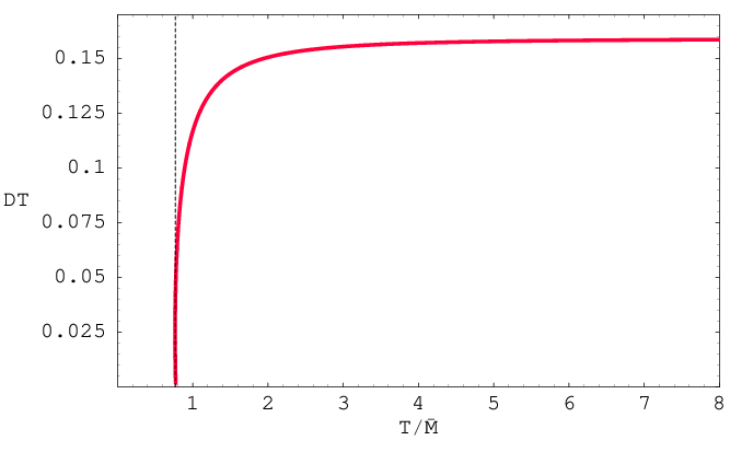
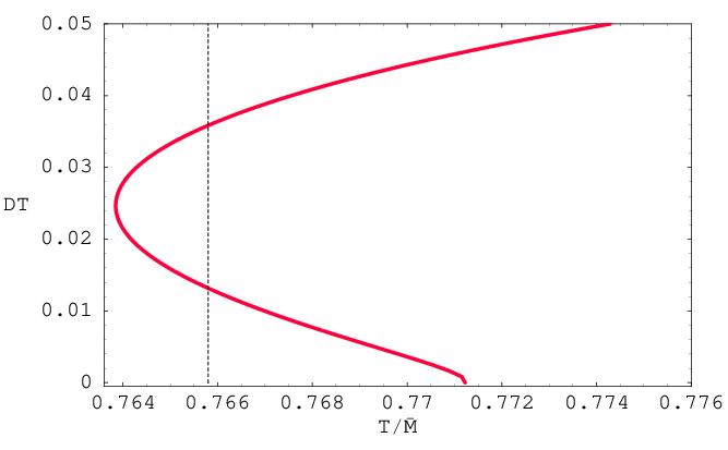
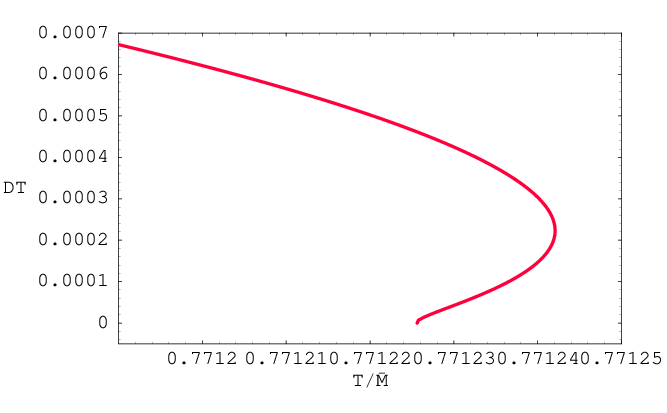
Using the numerical solutions for the embedding $\chi$ , we numerically integrated (5.104) to find $DT$ . The results are plotted in figs. 12 and 13. Fig. 12 clearly shows that asymptotically at high temperatures, $DT$ approaches $1/2\pi$ . This coincides with the result for the diffusion constant of R-charges in ${\cal N}=4$ SYM [16]. At a pragmatic level, this coincidence arises because both results are constructed from correlators of a Maxwell field in a AdS₅ black hole background. As the quark mass is increased, the induced geometry on the D7-brane deviates from that of the background geometry. Hence one finds a departure of $DT$ away from $1/2\pi$ as the ratio $T/\bar{M}$ decreases. Close to the phase transition, there is a rapid decrease and $DT=0.036\simeq 0.226/2\pi$ at the phase transition. If we continue following the black hole branch beyond the phase transition, $DT$ continues to fall and it also becomes a multi-valued function of temperature, as shown in fig. 13. The latter simply reflects the fact that multiple embeddings can be found for a single temperature in the vicinity of the critical solution.

5.2 Green-Kubo formula

As discussed in section 2.1, the diffusion constant may also be computed using the Green-Kubo formula (2.11) which relates the product of the diffusion constant $D$ and the susceptibility $\Xi$ to the slope of the vector spectral function ( $\ell=0$ ) for $\omega\to 0$ : $D\Xi=\lim_{\omega\to 0}{\swabfamily R}(\omega)/2\omega$ . The susceptibility is $\Xi=\partial n_{q}/\partial\mu|_{\mu=0}$ where $n_{q}$ is the charge density and $\mu$ is the chemical potential, both for fundamental matter (quarks or their supersymmetric generalization). In order to compute the susceptibility, one must consider the D3/D7 brane system with a finite chemical potential [38]. The susceptibility can be computed directly from eq. (2.22) of [38]

\tilde{\mu}=2\tilde{d}\int_{1}^{\infty}d\rho\,\frac{f\sqrt{1-\chi^{2}+\rho^{2}\dot{\chi}^{2}}}{\sqrt{\tilde{f}(1-\chi^{2})[\rho^{6}\tilde{f}^{3}(1-\chi^{2})^{3}+8\tilde{d}^{2}]}}\,,

(5.105)

which applies for any black hole embeddings. From the appendix of that paper, $\tilde{\mu}$ and $\tilde{d}$ are related to $\mu$ and $n_{\textrm{\tiny q}}$ via

\tilde{\mu}=\sqrt{\frac{2}{\lambda}}\,\frac{\mu}{T}\,,\qquad\tilde{d}=\frac{2^{5/2}}{N_{\textrm{\tiny f}}N_{\textrm{\tiny c}}\lambda^{1/2}}\,\frac{n_{\textrm{\tiny q}}}{T^{3}}\,.

(5.106)

Combining these definitions, we have

\frac{\partial\tilde{d}}{\partial\tilde{\mu}}=\frac{4}{N_{\textrm{\tiny f}}N_{\textrm{\tiny c}}T^{2}}\,\frac{\partial n_{\textrm{\tiny q}}}{\partial\mu}

(5.107)

which, interestingly, is independent of the ’t Hooft coupling $\lambda$ .

Note from eq. (5.105) that $\tilde{\mu}=0$ is equivalent to $\tilde{d}=0$ which means that we can calculate $\partial\tilde{\mu}/\partial\tilde{d}|_{\tilde{d}=0}$ from this equation and take the inverse for the desired derivative. Hence a straightforward calculation yields

\frac{\partial\tilde{\mu}}{\partial\tilde{d}}=2\int_{1}^{\infty}d\rho\,\frac{\rho^{6}f\tilde{f}^{4}(1-\chi^{2})^{4}\sqrt{1-\chi^{2}+\rho^{2}\dot{\chi}^{2}}}{\left(\tilde{f}(1-\chi^{2})[\rho^{6}\tilde{f}^{3}(1-\chi^{2})^{3}+8\tilde{d}^{2}]\right)^{3/2}}\,,

(5.108)

and evaluating at $\tilde{d}=0$ gives

\left.\frac{\partial\tilde{\mu}}{\partial\tilde{d}}\right|_{\tilde{d}=0}=2\int_{1}^{\infty}d\rho\,\frac{f\sqrt{1-\chi^{2}+\rho^{2}\dot{\chi}^{2}}}{\tilde{f}^{2}\rho^{3}(1-\chi^{2})^{2}}\,.

(5.109)

Combining eqs. (5.107) and (5.109), our final result is

\Xi\equiv\left.\frac{\partial n_{\textrm{\tiny q}}}{\partial\mu}\right|_{\mu=0}=\frac{N_{\textrm{\tiny f}}N_{\textrm{\tiny c}}}{4}\,T^{2}\,\left\{\ \left.\frac{\partial\tilde{\mu}}{\partial\tilde{d}}\right|_{\tilde{d}=0}\ \right\}^{-1}\,.

(5.110)

Note that in limit of massless quarks (i.e., $\chi=0$ ), these expressions have a simple form

\left.\frac{\partial\tilde{\mu}}{\partial\tilde{d}}\right|_{\tilde{d}=0}=\frac{1}{2}\,,\qquad\Xi=\frac{N_{\textrm{\tiny f}}N_{\textrm{\tiny c}}}{2}\,T^{2}\,.

(5.111)

Numerically evaluating the low frequency limit of the spectral function ${\swabfamily R}$ and the susceptibility (using (5.110) and (5.109)), we computed the diffusion constant using (2.11), and the results confirm those displayed in figure 12.

Further, if we combine (5.110) and (5.104), we are lead to write

D\,\Xi=\frac{(1-\chi_{0}^{2})^{3/2}}{4\pi}\,N_{\textrm{\tiny f}}N_{\textrm{\tiny c}}\,T\,,

(5.112)

which, in view of (2.11), provides a simple analytic expression for the low frequency ( $\omega\to 0$ ) limit of the vector spectral function:

{\swabfamily R}(\omega)=\frac{(1-\chi_{0}^{2})^{3/2}}{2\pi}N_{\textrm{\tiny f}}N_{\textrm{\tiny c}}T\omega+\cdots\,.

(5.113)

In a related analysis, the electric conductivity $\sigma$ of this system with fundamental quarks was recently computed from Ohm’s law using AdS/CFT techniques [39]. In the limit of vanishing quark density and small external electric field, the result of [39] reduces to our formula (5.112) above, as it should according to the generalized Einstein relation $\sigma/e^{2}=D\,\Xi$ . (Note that $e^{2}$ is set to one in the conventions of [39].)

5.3 Lowest quasinormal frequency (in the diffusion channel)

The final computation of the diffusion constant comes from examining the hydrodynamic dispersion relation, corresponding to the lowest quasinormal frequency. At small three-momentum $q$ , the diffusion constant can be extracted from: $\omega=-iDq^{2}+\mathcal{O}(q^{4})$ [17]. In principle, the calculation of the quasinormal mode spectrum from eq. (4.62) proceeds as follows: For $\rho\to\infty$ , eq. (4.62) implies that $E_{x}\simeq A+B\rho^{-2}$ for some constants $A,B$ . Normalizable modes will be those with $A=0$ . Hence one method to determine the quasinormal frequencies is to use a two-dimensional shooting method, i.e., solving (4.62) numerically with incoming wave boundary conditions at the horizon and then tuning the (complex) frequency to find a solution behaving as $\rho^{-2}$ asymptotically. For small $q$ we solved (4.62) for various $m$ to determined the lowest quasinormal frequency and our results for the diffusion constant are identical to those plotted in fig. 12.

6 Discussion

In this paper, we used holography to investigate various aspects of the high temperature phase of an ${\cal N}=2$ super-Yang-Mills theory with fundamental matter. The holographic description consists of probe D7-branes in the near-horizon background of D3-branes (in the limit of large- $N_{\textrm{\tiny c}}$ and large- $\lambda$ with fixed $N_{\textrm{\tiny f}}$ ). In the high temperature phase, the D7-branes extend through the event horizon of the AdS₅ black hole, which describes the theory at finite temperature. In [7, 10], this phase was denoted as the black hole branch since the metric induced on the worldvolume of the D7-branes is itself a black hole. Even though the latter geometry no longer obeys Einstein’s equations, the analysis of the hydrodynamic physics found previously for bulk fields, e.g., [40], is readily transferred to the worldvolume fields on the D7-brane. Hence we were able to examine the spectral function for various mesonic operators in section 4, following [30, 18], and we calculated the diffusion constant for the quark charge in section 5, adapting techniques from [17, 16].

As reviewed in section 3, the induced geometry (3.39) on the D7-brane is determined by first solving for the embedding profile from eq. (3.41) with appropriate asymptotic boundary conditions (3.42). Given the complexity of eq. (3.41), these geometries are only known in general from numerical integration. However, there is one particularly simple case, namely that of zero quark mass. In this case, the embedding is trivial, i.e., $\chi=0$ everywhere, and the induced geometry (3.39) is precisely that of (the direct product of) an AdS₅ black hole (with a constant $S^{3}$ ). Hence our analysis of sections 4.1 and 5 reduces to studying a Maxwell field in an AdS₅ black hole geometry and the results precisely match those found previously for bulk gauge fields. For example, the quark diffusion constant (with $M_{\textrm{\tiny q}}=0$ ) matches precisely with the $R$ -charge diffusion constant calculated in [16, 17]. Further the new analytic expression of the vector spectral function presented in section 2.3 was extended to an analytic result for all of the higher- $\ell$ modes of the worldvolume vector.

As the quark mass is increased away from zero (or $T/M_{\textrm{\tiny q}}$ decreases to finite values), the induced black hole geometry on the D7-brane begins to deviate from that of the background. In particular, the main differences arise near the event horizon where $\chi$ is largest. For example, eq. (3.39) shows that the size of the $S^{3}$ and hence the induced horizon area shrinks as $\chi_{0}$ grows. Hence the physical properties of the fundamental fields were seen to depart (dramatically in some cases) from the standard results with the growth of the quark mass. Recall that some of the most interesting behaviour appeared as $\chi_{0}\rightarrow 1$ , i.e., approaching the critical solution for which the effective horizon area vanishes. Hence this behaviour can be seen as a precursor of the phase transition to the low temperature phase or the Minkowski branch, in which the D7-brane smoothly closes off above the event horizon.

In the low temperature phase (and in the limit of large $N_{\textrm{\tiny c}}$ ), the spectrum of mesons is characterized by a discrete set of stable states [11, 10] and the spectral function is a series of $\delta$ -function peaks, as illustrated in fig.2a. A derivation of the spectral function for the scalar meson at $T=0$ appears in appendix B. These mesonic states correspond to open string excitations which are essentially living at the minimum radius of the D7-brane. Since in the high temperature phase the D7-branes extends through the event horizon, these states are destabilized. In this phase, the spectrum can be characterized by a discrete set of quasinormal modes in the effective black hole metric induced on the D7-brane. The spectral functions calculated in section 4 reveal interesting information about this quasinormal spectrum. We focussed on three particular operators, which are bilinears of the fundamental fields – the details appear in appendix A – corresponding vector, pseudoscalar and scalar channels.

The behaviours of the vector and pseudoscalar spectral functions are very similar, as can be seen in figures 5 and 8. The following physical picture emerges from these plots: At very high temperatures, the spectral function closely resembles that for a vector in ${\cal N}=4$ SYM. (Of course, as discussed above, the bulk and worldvolume vector results are identical for $T/M_{\textrm{\tiny q}}\rightarrow\infty$ .) In this regime, the spectral functions show essentially no structure and the eigenfrequencies of quasinormal modes must all be deep in the (lower) complex plane. As the temperature decreases (with fixed quark mass), both the real and imaginary parts of a given quasinormal frequency decrease but the formation of peaks in the spectral function suggests that the imaginary part decreases more rapidly. At temperatures just above the phase transition, there are vector and pseudoscalar quasiparticles. Continuing along the black hole branch to even lower temperatures beyond the phase transition (i.e., following the black hole line through $A_{1}$ in fig. 4), peaks grow very sharp and even more prominent indicating that the quasinormal modes have $\textrm{Re}(\omega)\gg\textrm{Im}(\omega)$ in this regime.

Appendix D presents a complementary discussion which reaches the same conclusion. Plots of the effective potential for the pseudoscalar (and vector) excitations in appendix D show a finite potential barrier developing at intermediate values of the radius as $\chi_{0}\to 1$ . This suggests the existence of metastable states in the corresponding Schroedinger problem which, as discussed in the appendix, would correspond to a quasinormal frequency with $\Gamma\ll\Omega$ i.e., the eigenfrequency approaches the real axis in this regime. Of course, while this intuitive picture developed from the effective potential matches the behaviour of the spectral functions discussed above, it only gives a very schematic picture of the quasinormal spectrum. Hence it would be interesting to develop more detailed picture with a full calculation of the quasinormal modes [36].

If we examine the positions of the peaks in the spectral functions more closely as the black hole embedding approaches the critical solution, it appears that the real parts of the quasinormal frequencies roughly match with the spectrum of the lowest (vector and pseudoscalar) mesons on a near-critical Minkowski embedding. Hence one notable feature of the spectral functions is that as $\chi_{0}\to 1$ , the peaks are becoming sharper but also more closely spaced and moving towards lower frequencies. For example, in figure 8, the peaks in the $\chi_{0}=0.9999$ line are much more closely spaced than those in the $\chi_{0}=0.99$ line. This behaviour is similar to what is seen for the $\delta\phi$ spectrum for near-critical Minkowski embeddings: For these near-critical embeddings, the tower of masses appears to be collapsing to the mass of the lowest meson – see fig. 7 in [10]. As the phase transition occurs well away from the critical solution (i.e., $\chi_{0}=0.94$ versus 1), the positions of the spectral peaks are not closely matched with the corresponding meson spectrum for the Minkowski embedding at the phase transition. Of course, both spectra still characterized by the same general mass scale, as given in eq. (3.43).

We also examined the spectral functions for $\ell>0$ in vector and pseudoscalar channels. These modes of the worldvolume fields correspond to higher dimension operators in the field theory, which are charged under the internal symmetry group $SO(4)=SU(2)\times SU(2)$ – see the discussion in appendix A. For these modes, the results are qualitatively similar to those for $\ell=0$ as one approaches the critical embedding. However, the rate at which the quasinormal frequencies approach the real axis is much slower – that is, the spectral functions only develop pronounced peaks very close to $\chi_{0}=1$ . In fact, these peaks are already washed out at the phase transition, i.e., $\chi_{0}=0.94$ . Hence the corresponding mesons with $\ell>0$ do not survive as quasiparticles through the phase transition. The analogous observation applies to the excited mesons with $\ell=0$ and $n\geq 1$ . Examining the spectral functions in figs. 5 and 8, one finds that only the first peak remains pronounced at $\chi_{0}=0.94$ . Hence it seems that only the ground state mesons (with $n=0=\ell$ ) can be said to survive the phase transition as quasiparticles. However, even these resonances have disappeared in the quark-gluon plasma by $\chi_{0}\simeq 0.8$ or $T\simeq 1.1T_{\textrm{\tiny fund}}$ , where $T_{\textrm{\tiny fund}}$ is the temperature of the phase transition.

As shown in figures 9 and 10, the behaviour of the scalar spectral function is qualitatively different from that found in the vector and pseudoscalar channels, shown in figs. 5 and 8. As before, at high temperatures, the spectral function shows no distinguished structure, indicating that the quasinormal eigenfrequencies are all deep in the (lower) complex plane. As the temperature decreases, a small peak develops near the origin although it is still not very prominent at the phase transition. However, continuing to the D7-brane embeddings on the black hole branch for temperatures below the phase transition, this single peak grows and becomes extremely sharp and centred at $\omega=0$ , precisely at the first kink in the free energy, i.e., $\chi_{0}=0.9621$ . Beyond this point, the peak decays and moves away from $\omega=0$ . Our interpretation of this behaviour is that the lowest (pair) of quasinormal frequencies approaches the origin and actually crosses the real axis at the point $A_{2}$ in fig. 4. Continuing beyond this point, this eigenfrequency moves into the upper half plane, where it actually corresponds to an unstable mode.

This interpretation of the behaviour of the scalar spectral function is confirmed by the qualitative analysis of the corresponding quasinormal modes in appendix D. Examining the effective potential for the scalar excitations shows that a negative potential well develops and grows as $\chi_{0}\to 1$ . As discussed in the appendix, when this well is large enough, it can support long-lived ‘bound’ states for which (the real part of) the effective energy is negative. These modes are distinguished since $\Gamma^{2}>\Omega^{2}$ and further $\Gamma<0$ , so that these bound states correspond to instabilities of the D7-brane. The spike (or pole) at $\omega=0$ in the scalar spectral function discussed above results from the formation of the first bound state where the eigenfrequency crosses the real axis. Ref. [36] studied the quasinormal modes in this channel and developed a qualitative picture which is in agreement with our results.

Recall that the thermodynamic discussion of section 3.1 predicted that the system should become unstable at the point $A_{2}$ in fig. 4 because the specific heat of the black hole branch becomes negative there. Hence our analysis above is in precise agreement with this result and it shows that the instability corresponds to unstable ‘quasinormal’ modes appearing on the D7-branes.

In fact, we found the scalar spectral function also displays a spike at $\omega=0$ at the second kink in the free energy, i.e., $\chi_{0}=0.99973885$ . Hence it appears that the second lowest quasinormal mode becomes unstable at this point. It is natural to conjecture then that each time the free energy turns, a new ‘tachyonic’ mode appears in the scalar spectrum. In fact, the spectrum of scalar mesons on the Minkowski branch was found to display precisely this behaviour [10].

Again the spectral functions of mesonic operators which we calculated exhibited a number of interesting features, which had a clear interpretation in terms of the spectrum of quasinormal modes. It would, of course, be interesting to confirm these behaviours by a detailed investigation of the quasinormal modes, as was begun in [36]. In the present paper, the spectral functions were only calculated for zero spatial momentum for computational simplicity. So another natural extension of this work is to consider the behaviour at nonvanishing spatial momentum. In particular, the spectral functions for general time-like and light-like four-momentum can be used to calculate photon and dilepton production rates, respectively [13]. An analysis of these results for the present ${\cal N}=2$ gauge theory has been made recently [41].

The other main result of this paper was the calculation of the diffusion constant for the quark charge. We used a number of techniques developed for bulk black holes in the calculation of the $R$ -charge diffusion constant in the ${\cal N}=4$ theory: the membrane paradigm method [17], the Green-Kubo formula [16] (which for us relied on previous studies of this system at finite quark density [38]), and the lowest quasinormal frequency [17]. It is gratifying that as demanded by the internal consistency of the holographic framework, all three of these independent calculations yield the same results [42], which are shown in figure 12.

At very high temperatures (i.e., $T/\bar{M}\gg 1$ ), the diffusion constant approaches $2\pi D\,T=1$ , which as discussed above matches the $R$ -charge diffusion constant for the ${\cal N}=4$ super-Yang-Mills theory [17]. As $T/\bar{M}$ decreases, the product $D\,T$ decreases. Intuitively, we might understand this result as the rate of diffusion decreasing at a fixed temperature when the quark mass is increased. In fact, the decrease is remarkably small at first, e.g., $2\pi D\,T=0.9$ at $T/\bar{M}\simeq 1.5$ . However, figure 12 then shows a dramatic decline as we approach the phase transition at $T/\bar{M}=0.7658$ . At the phase transition, $2\pi D\,T\simeq 0.226$ , but if we continue following the black hole branch it appears that $D\,T$ continues to decrease and would vanish at the critical embedding. The membrane paradigm approach to calculating $D$ , as described in section 5.1, provides a straightforward understanding of this vanishing from the bulk perspective. Examining the expression in eq. (5.104), we see that in the critical limit, the integral remains finite but the prefactor vanishes because $\sqrt{-g}\to 0$ . Hence the dominant effect which causes $D$ to decrease is the reduction of the effective horizon area of the brane geometry (3.39) as we approach the critical embedding. That is, $(1-\chi_{0}^{2})\to 0$ in advancing toward the critical embedding. Further, this area vanishes precisely at the critical embedding confirming that $D$ should vanish there.

We have considered the ${\cal N}=2$ gauge theory to have $N_{\textrm{\tiny f}}$ flavours of quarks. Hence it is worth noting that the results for the quark diffusion constant in the present holographic framework are independent of both $N_{\textrm{\tiny f}}$ and $N_{\textrm{\tiny c}}$ . Of course, the same independence of $N_{\textrm{\tiny c}}$ was seen with the $R$ -charge [17]. This must certainly arise because we are working in the limit of large $N_{\textrm{\tiny c}}$ and large $\lambda$ .

There has also been a great deal of interest in the diffusion of ‘heavy quarks’ in holographic theories recently [46, 43, 44] – see also [45] and the references therein. In the present context, this simply refers to the quark diffusion constant in the low temperature phase where the D7-branes only approach to some finite distance away from the black hole horizon. In the low temperature or Minkowski embedding phase, a quark is represented by a fundamental string stretching between the D7-brane and the horizon. As such, a heavy quark is holographically represented by a macroscopic object (on a similar footing with the probe D7-branes) and classically this object will remain at rest (i.e., it does not ‘diffuse’). It is only when semiclassical effects are taken into account that the heavy quarks diffuse through the appearance of Hawking radiation from the effective black hole metric induced on the string worldsheet [43]. This process should be contrasted with the diffusion process in the high temperature phase which we have been considering here. As stressed above, in this phase the induced metric on the D7-brane is a black hole metric and so if quark number is injected into the system, the holographic description of diffusion is simply the classical process of the corresponding worldvolume excitations falling towards the event horizon. Given these two disparate descriptions, it is not surprising that the diffusion constant takes a qualitatively and quantitatively different form in the two phases. In the low temperature phase, the diffusion constant is governed by the heavy quark result[46, 43]¹³¹³ 13 Note we present this result with the same normalisation for the ’t Hooft coupling used throughout this paper. Ref. [46] uses a convention such that $\tilde{\lambda}=2\lambda$ . This difference arises from the implicit normalisation of the $U(N_{\textrm{\tiny c}})$ generators: Tr( $T_{a}\,T_{b})=d\,\delta_{ab}$ . The standard field theory convention used in [46] is $d=1/2$ while our choice is $d=1$ , as is prevalent in the D-brane literature.

2\pi\,D\,T=\sqrt{8/\lambda}\,.

(6.114)

On the other hand, after the transition to the high temperature phase, we found above that $2\pi\,D\,T=O(1)$ . Note that the holographic analysis applies for strong ’t Hooft coupling (i.e., $\lambda\gg 1$ ) and so these results show the expected suppression of quark diffusion in the low temperature phase.

We comment on a possible puzzle with the above description of the diffusion of heavy quarks as due to semiclassical Hawking radiation. As such, the diffusion constant would be expected to vanish in the limit $\hbar\to 0$ for the bulk theory. Now the standard AdS/CFT dictionary would associate Planck’s constant $\hbar$ in the bulk supergravity with $1/N_{\textrm{\tiny c}}$ in the dual gauge theory [4]. However, above, we see the result (6.114) is seen to be independent of $N_{\textrm{\tiny c}}$ and $D$ certainly does not vanish in the limit $N_{\textrm{\tiny c}}\to\infty$ . The resolution of this puzzle is that we have misidentified the correct ‘semiclassical’ nature of the diffusion process here. Above we observed that the heavy quarks diffuse because of the appearance of Hawking radiation in the effective field theory on the string worldsheet dual to such heavy quark. That is, the ‘fields’ on the worldsheet are the transverse coordinates describing the embedding of the string and so fluctuations in these fields (arising from Hawking radiation) corresponds to fluctuations in the position of the quark (i.e., diffusion of the quark). Now as usual, $\hbar$ for the worldsheet theory is identified with the inverse string tension, $\alpha^{\prime}=\ell_{\textrm{\tiny s}}^{2}$ . More correctly, the dimensionless $\hbar$ in the nonlinear sigma model one the worldsheet is identified with the ratio of $\alpha^{\prime}$ and the background curvature scale, i.e., $\hbar_{ws}\simeq\ell_{\textrm{\tiny s}}^{2}/L^{2}\simeq 1/\sqrt{\lambda}$ . Now we see this physical picture matches precisely with the calculated result (6.114) and the limit $\lambda\to\infty$ is the semiclassical limit on the string worldsheet.

The results for the diffusion constant in both the high and low temperature phases are combined in figure 14, where $2\pi D\,T$ is shown as a function of $\lambda$ (for fixed $M_{\textrm{\tiny q}}/T$ ). The thick black curve shows a canonical result for the ${\cal N}=2$ gauge theory, which we are displaying for $M_{\textrm{\tiny q}}/T=200$ . The diffusion constant starts at very large values on the left in nearly perturbative results. The dashed ‘perturbative’ line is the extrapolation of the perturbative calculation of [47] for ${\cal N}=4$ super-Yang-Mills at large $N_{\textrm{\tiny c}}$ . As the curve shows, we expect $D\,T$ to make a transition to the $\lambda^{-1/2}$ behaviour of heavy quarks in the low temperature phase. If the quark mass was infinite, this behaviour would extend out to infinite ’t Hooft coupling. However, for a finite mass, increasing $\lambda$ eventually takes the system to the high temperature phase. It would be interesting to understand the corrections to the heavy quark result (6.114), as we approach the phase transition. For $M_{\textrm{\tiny q}}/T=200$ , the latter occurs at $\lambda\simeq 9.4\times 10^{4}$ [7, 10]. At this first order phase transition, $2\pi\,D\,T$ jumps discontinuously up to the ‘light quark’ curve at $2\pi\,D\,T=0.226$ and it quickly reaches the asymptotic value of 1 as $\lambda$ continues to increase.

Much of the recent interest in holographic calculations of the diffusion constant was generated by the possibility to compare these strong coupling results with experimental results for the QCD quark-gluon plasma measured at RHIC [48]. It is interesting then to place the RHIC results in the context of the phenomenology of the ${\cal N}=2$ gauge theory studied here. The bar labeled RHIC corresponds to $\alpha_{strong}=0.5$ (or $\lambda=3\pi$ ) and the range $2\pi\,D\,T=3\sim 12$ , which is used in fitting the observed nuclear modification factor and elliptic flow amplitude for heavy (charm) quarks – see [48] for details. This value of the ’t Hooft coupling is well away from the light quark behaviour of our canonical theory but also lies in an intermediate regime between the heavy quark and perturbative regimes. Hence a direct comparison of either approach for the ${\cal N}=2$ theory to the experimental data for QCD is difficult [47, 49]. We emphasize that in this intermediate region our canonical curve is simply an ‘artistic’ impression of the cross-over between these two regimes.

For the canonical theory, we chose $M_{\textrm{\tiny q}}/T=200$ so that the phase transition between the low and high temperature regimes took place for a value of $\lambda$ that we could confidently characterize as strong coupling. So we extend our discussion of RHIC results by noting that the charm quark has a mass of roughly $1500$ MeV while the temperatures achieved in the RHIC collisions are in the regime $250$ MeV. Hence in these experiments, we are considering $M_{\textrm{\tiny q}}/T\simeq 6$ . As illustrated in figure 14, the effect of reducing this ratio is to slide the light quark curve to the left. That is, the phase transition occurs at smaller and smaller values of $\lambda$ , e.g., $\lambda_{c}\simeq 85$ for $M_{\textrm{\tiny q}}/T\simeq 6$ . However, it seems that this critical value is still well away from the value of the coupling relevant for RHIC. Further it seems that the same will still be true for charm quarks even at the higher temperatures that might be achieved in the future at the LHC. Thus it is unlikely that a dramatic jump in the diffusion constant, such as that seen for our canonical theory, will appear in these experiments. It is noteworthy that in any event, the experimentally favoured values of the heavy quark diffusion constant are in fact above those calculated in the high temperature phase. Hence it would seem that a QCD phase transition would be characterized by a sudden decrease rather than a sudden increase in the diffusion constant.

While our results for the diffusion constant do not seem relevant for ‘heavy quarks’, they might be considered as that for ‘light quarks’ in QCD. Note that our holographic model gave $2\pi\,D\,T\leq 1$ where the effect of a finite quark mass was to give a slight (less than order one) reduction below the asymptotic value of 1. Appendix E extends the computation of the diffusion constant described in section 5.1 to more general holographic theories. In particular, figure 18 shows the results for the D4/D6-brane system, which is the basis for the construction of one holographic model which mimics QCD at large $N_{\textrm{\tiny c}}$ [50]. The results are similar to those above with $2\pi\,D\,T\leq 3/2$ with finite mass effects giving a small reduction from the asymptotic value. Another interesting holographic model of a QCD-like theory comes from introducing D8 and anti-D8 probe branes in a D4-brane background [51]. The resulting diffusion constant is simply $2\pi\,D\,T=1$ . In this model, the current quark mass is fixed vanish and so no finite mass effects appear. We might also recall the results for the $R$ -charge diffusion constants $2\pi\,D\,T=1$ and 3/4, for the near-extremal D3- and D4-brane backgrounds [17]. Hence in all these cases then, we find that the calculations yield $2\pi\,D\,T=O(1)$ . This might suggest that in QCD, the diffusion constant associated with the light quarks falls dramatically at strong coupling, as compared to the perturbative results [52], but that they should saturate around this level. One might note then that these diffusion constants would be smaller than for heavy quarks at presently accessible energies but not much smaller. However, we must recall that these calculations are all performed at large $\lambda$ and large $N_{\textrm{\tiny c}}$ (with $N_{\textrm{\tiny f}}/N_{\textrm{\tiny c}}\ll 1$ ) and so it would of course be interesting to understand the corrections to these results at finite $\lambda$ and finite $N_{\textrm{\tiny c}}$ .

In the present study, we focussed on calculating the diffusion constant for the overall quark charge. Of course, with $N_{\textrm{\tiny f}}$ flavours of quarks with identical masses, the ${\cal N}=2$ gauge theory has a global $U(N_{\textrm{\tiny f}})$ flavour symmetry and in the dual gravity description, the worldvolume theory of the D7-brane contains a nonabelian $U(N_{\textrm{\tiny f}})$ gauge field. Our calculations have only considered the diagonal $U(1)$ component of this gauge field. However, as noted in appendix A, one can easily examine the nonabelian $SU(N_{\textrm{\tiny f}})$ flavour currents with the corresponding components of the worldvolume gauge field – see, e.g., eq. (A.120). Now in principle, we would describe the diffusion of the full set of flavour currents with a diffusion matrix $D_{ab}$ , rather than a single constant. However, our calculations of the diffusion constant in section 5 only relied on knowing the quadratic action for the dual gauge field and hence the nonabelian character of the gauge fields would play no role. Hence the diffusion matrix is, in fact, diagonal: $D_{ab}=D\,\delta_{ab}$ where $D$ is precisely the constant determined for the $U(1)$ charge. On general grounds, this is of course the expected result for the ${\cal N}=2$ gauge theory in the absence of any chemical potentials. With a nonvanishing chemical potential, the diffusion matrix will not take this simple form [53]. Similar comments to those above also apply for extending our calculations of the spectral function to operators that are no longer $SU(N_{\textrm{\tiny f}})$ singlets.

Acknowledgments.

We thank Alex Buchel, Jaume Gomis, Pavel Kovtun, Peter Langfelder and David Mateos for helpful discussions and comments. Research at the Perimeter Institute is supported in part by the Government of Canada through NSERC and by the Province of Ontario through MRI. We also acknowledge support from an NSERC Discovery grant (RCM), NSERC Canada Graduate Scholarship (RMT) and the Canadian Institute for Advanced Research (RCM,RMT). Research at the KITP was supported in part by the NSF under Grant No. PHY05-51164. RCM would like to thank the organizers of Strings 2006 and String Phenomenology 2006 for the opportunity to present some of the results discussed here.

Appendix A Holographic dictionary

In sections 4.1 and 4.2, we focussed on three worldvolume fields: the gauge field $A_{\mu}$ and the embedding coordinates $\chi$ and $\phi$ . We made use of the fact that the asymptotic behaviour of these D7-brane fields has a direct translation in terms of hypermultiplet operators in the gauge theory. In this appendix, we elucidate this holographic dictionary in more detail. Our discussion provides more detail on the pseudoscalar operator since the other two operators have already been considered in some detail in [10, 38].

Let us remind the reader that a hypermultiplet consists of two Weyl fermions $\psi,\tilde{\psi}$ and two complex scalars $q,\tilde{q}$ . Of these, $\psi$ and $q$ transform in the fundamental of the $SU(N_{\textrm{\tiny c}})$ gauge group, while $\tilde{\psi}$ and $\tilde{q}$ transform in the antifundamental. Further, with $N_{\textrm{\tiny f}}$ flavours (of equal mass), the hypermultiplets transform under a global $U(N_{\textrm{\tiny f}})\simeq SU(N_{\textrm{\tiny f}})\times U(1)_{\textrm{\tiny q}}$ symmetry. The charges of the fields under the diagonal $U(1)_{\textrm{\tiny q}}$ are +1 for $\psi$ and $q$ and –1 for $\tilde{\psi}$ and $\tilde{q}$ . Hence the $U(1)_{\textrm{\tiny q}}$ charge naturally counts the net number of quarks in a given state. Here and below, we follow the notation of [54].

The operators dual to $A_{\mu}$ , $\chi$ and $\phi$ can be determined by considering the interactions of the open strings on the D3/D7 array (3.35) before the decoupling limit [55], in analogy with the closed strings. Such an exercise leads to the following operators:

$\displaystyle A_{\mu}\$	$\displaystyle\leftrightarrow$	$\displaystyle\ J^{\mu}_{\textrm{\tiny q}}=\bar{\psi}\bar{\sigma}^{\mu}\psi+\tilde{\psi}\sigma^{\mu}\tilde{\psi}^{\dagger}-i\left({q}^{\dagger}{\cal D}^{\mu}{q}-({\cal D}^{\mu}{q})^{\dagger}{q}\right)-i\left(\tilde{q}\,({\cal D}^{\mu}\tilde{q})^{\dagger}-{\cal D}^{\mu}\tilde{q}\,\tilde{q}^{\dagger}\right)\,,$	(A.115)
$\displaystyle\chi\$	$\displaystyle\leftrightarrow$	$\displaystyle\ {\cal O}_{\textrm{\tiny m}}=i\tilde{\psi}\psi+\tilde{q}(M_{\textrm{\tiny q}}+\sqrt{2}\Phi^{1})\tilde{q}^{\dagger}+{q}^{\dagger}(M_{\textrm{\tiny q}}+\sqrt{2}\Phi^{1}){q}+h.c.\,,$	(A.116)
$\displaystyle\phi\$	$\displaystyle\leftrightarrow$	$\displaystyle\ {\cal O}_{\phi}=\tilde{\psi}\psi+i\sqrt{2}\,\tilde{q}\,\Phi^{1}\,\tilde{q}^{\dagger}+i\sqrt{2}\,{q}^{\dagger}\,\Phi^{1}\,{q}+h.c.\,.$	(A.117)

Note that $\Phi^{1}$ , a complex scalar in the ${\cal N}=4$ supermultiplet, as well as $M_{q}$ , appear in the scalar terms after solving for the auxiliary field constraints within the full coupled theory. Note that both these operators have conformal dimension¹⁴¹⁴ 14 This dimension applies in the UV where the effects of quark mass are negligible and the theory becomes conformal. $\Delta=3$ , which matches the standard prescription for the powers of $\rho$ appearing in the asymptotic behaviour of the fields – see below.

Let us comment on the derivation of ${\cal O}_{\phi}$ . The mass term for the hypermultiplet fields originates from the following superpotential term

i\sqrt{2}\,\int d^{2}\theta\,\left(\tilde{Q}\,\Phi_{7,7}\,Q-h.c.\right)

(A.118)

where $\tilde{Q}$ and $Q$ are chiral superfields containing $(\tilde{q},\tilde{\psi})$ and $(q,\psi)$ , respectively. These hypermultiplet fields appear as ground states of the 3-7 and 7-3 strings while, as the subscript indicates, the superfield $\Phi_{7,7}$ describes a particular set of massless modes in the 7-7 string sector. In particular, the lowest component of $\Phi_{7,7}$ is a complex scalar describing the transverse fluctuations of the D7-brane position, i.e.,

\Phi_{7,7}=\frac{1}{\sqrt{2}}\left(\frac{X^{8}+i\,X^{9}}{2\pi\ell_{s}^{2}}\right)+\cdots\ .

(A.119)

for the orientation in eq. (3.35). After the decoupling limit, this is no longer a dynamical field in the gauge theory but its expectation value sets the mass of the hypermultiplets, i.e., $\langle\Phi_{7,7}\rangle=M_{\textrm{\tiny q}}/\sqrt{2}$ . One sees from eq. (A.119) that the geometric angle $\phi$ appearing in our construction of the D7-brane embeddings in section 3 corresponds precisely to the phase of the complex field $\Phi_{7,7}$ . Hence in deriving ${\cal O}_{\phi}$ , we consider a phase rotation with the given expectation value for $\Phi_{7,7}$ in the Lagrangian (A.118). The resulting variation yields $\delta{\cal L}=\delta\phi\,M_{\textrm{\tiny q}}\,{\cal O}_{\phi}$ and so we have divided by the factor of $M_{\textrm{\tiny q}}$ in defining the operator given in eq. (A.117).

Recall that the full flavour symmetry is $U(N_{\textrm{\tiny f}})$ , which of course matches the worldvolume gauge symmetry of the D7-branes. The current $J^{\mu}_{\textrm{\tiny q}}$ is the conserved current corresponding to the diagonal $U(1)_{\textrm{\tiny q}}$ of this global symmetry, i.e., $J^{t}_{\textrm{\tiny q}}$ is the quark charge density. Our discussion can easily extended to the $SU(N_{\textrm{\tiny f}})$ symmetry by considering the nonAbelian gauge fields on the D7-brane. The corresponding flavour currents would be

	$\displaystyle A^{a}_{\mu}\$	$\displaystyle\leftrightarrow$	$\displaystyle\ (J^{a})^{\mu}=\left(T^{a}\right)_{i}{}^{j}\left[\bar{\psi}^{i}\bar{\sigma}^{\mu}\psi_{j}+\tilde{\psi}^{i}\sigma^{\mu}\tilde{\psi}^{\dagger}_{j}-i\left({q}^{\dagger i}{\cal D}^{\mu}{q_{j}}-({\cal D}^{\mu}{q})^{\dagger i}{q}_{j}\right)\right.$		(A.120)
			$\displaystyle\left.\qquad\qquad\qquad\qquad\qquad\qquad\qquad\qquad\qquad-i\left(\tilde{q}^{\,i}\,({\cal D}^{\mu}\tilde{q})^{\dagger}_{j}-{\cal D}^{\mu}\tilde{q}^{\,i}\,\tilde{q}^{\dagger}_{j}\right)\right]\,,$		(A.120)

where $T^{a}$ are (Hermitian) generators of $SU(N_{\textrm{\tiny f}})$ and we have restored explicit flavour indices on the fields. With the operators ${\cal O}_{\textrm{\tiny m}}$ and ${\cal O}_{\phi}$ , we have also focussed on the $SU(N_{\textrm{\tiny f}})$ neutral terms but it would be straightforward to extend these to a more general discussion. For example, in general $\Phi_{7,7}$ transforms in the adjoint of $U(N_{\textrm{\tiny f}})$ and so one can easily chose a more elaborate mass matrix rather than one proportional to the identity as above.

Recall the equation of motion (3.41) for $\chi$ implies that asymptotically

\chi=\frac{m}{\rho}+\frac{c}{\rho^{3}}+\cdots\,.

(A.121)

The dimensionless constants $m$ and $c$ are related to the quark mass and condensate as [10]:

	$\displaystyle M_{\textrm{\tiny q}}$	$\displaystyle=$	$\displaystyle\frac{1}{2}\sqrt{\lambda}\,T\,m\,,$		(A.122)
	$\displaystyle\langle{\cal O}_{\textrm{\tiny m}}\rangle$	$\displaystyle=$	$\displaystyle-\frac{1}{8}\sqrt{\lambda}\,N_{\textrm{\tiny f}}\,N_{\textrm{\tiny c}}T^{3}\,c\,.$		(A.123)

As presented here, this dictionary was established for a constant coefficient (i.e., the mass) and uniform expectation value of the operator ${\cal O}_{\textrm{\tiny m}}$ . However, the same relationships also apply in considering correlators where $M_{\textrm{\tiny q}}$ is shifted with a general space- and time-dependent coefficient or source $\mu(x)$ . In section 4.2, we express the relevant correlators in terms of variations $\delta\theta(x,\rho)$ (or its Fourier transform along the $x^{\mu}$ directions). Given that $\chi\equiv\cos\theta$ , we have $\delta\theta\simeq-\delta\chi$ asymptotically where $\chi$ approaches zero. Hence, as confirmed from eq. (4.87), $\delta\theta$ has the following the asymptotic behaviour:

\delta\theta(x,\rho)=\frac{\delta\theta_{0}(x)}{\rho}+\frac{\Theta(x)}{\rho^{3}}+\cdots\,,

(A.124)

The source term is related to the first coefficient above as in eq. (A.122) (up to a sign): $\mu(x)=-\frac{1}{2}\sqrt{\lambda}\,T\,\delta\theta_{0}(x)$ . Similarly the induced expectation value and $\Theta(x)$ are related as in eq. (A.123), again up to an overall sign.

Ref. [38] investigated the present holographic theory at finite quark density and so established a similar dictionary for the (time component of the) worldvolume gauge field. With the asymptotic behaviour

A_{t}=\mu-\frac{\tilde{\sigma}}{\rho}+\cdots\,,

(A.125)

it was found that $\mu$ is precisely the chemical potential or the coefficient of the charge density operator $J_{q}^{t}$ and the quark density was given by

n_{q}\equiv\langle\,J_{q}^{t}\,\rangle=\frac{1}{4}N_{\textrm{\tiny f}}N_{\textrm{\tiny c}}\,T^{2}\,\tilde{\sigma}\,.

(A.126)

Again these relations were originally established for a constant chemical potential and uniform quark density but they still apply for more general configurations. In particular for the correlators of section 4.1, we consider more general gauge field configurations with asymptotic behaviour

A_{\mu}=\Sigma_{\mu}(x)+\frac{\sigma_{\mu}(x)}{\rho}+\cdots\,.

(A.127)

In this case, $\Sigma_{\mu}$ corresponds to the (space- and time-dependent) coefficient of the current operator $J_{q}^{\mu}$ and the induced expectation values are given by

\langle J_{q}^{\mu}(x)\rangle=\frac{1}{4}N_{\textrm{\tiny f}}N_{\textrm{\tiny c}}\,T^{2}\,\sigma^{\mu}(x)\,.

(A.128)

Note that here the index on $\sigma^{\mu}$ is raised with $\eta^{\mu\nu}$ , the inverse metric in the CFT.¹⁵¹⁵ 15 Note that while the calculation of the spectral function in section 4.1 is presented in terms of the gauge-invariant field strengths $F_{\mu\nu}$ , this was simply choice of convenience and the final spectral function corresponds to that for current in eq. (A.115).

Now we would like to turn to the holographic dictionary for the $\delta\phi$ modes. From the equation of motion (4.86) and the asymptotic behaviour of $\chi$ given in eq. (A.121), we can determine that $\delta\phi$ has the following asymptotic behaviour

\delta\phi(x,\rho)=\delta\phi_{0}(x)+\frac{\Phi(x)}{\rho^{2}}+\cdots\,.

(A.129)

From eq. (A.119), we saw that the geometric angle $\phi$ appearing in the D7-brane embeddings corresponds precisely to the phase of the complex field $\Phi_{7,7}$ . Hence $\delta\phi_{0}$ corresponds to a fluctuation in the phase of the hypermultiplet mass term. As usual, the dimensionless constant $\Phi$ is proportional to the induced expectation value of ${\cal O}_{\phi}$ but we would still need establish the precise constant of proportionality.

To establish the latter relationship, it is natural to frame the discussion in terms of the thermal partition function – see [38], for example.¹⁶¹⁶ 16 In principle then this discussion only concerns space- but not time-dependent sources. However, the following results apply for the general case including time dependence. The source potential $\delta\phi_{0}$ enters the partition function as

\exp\left[-\beta\,F(\beta,\delta\phi_{0})\right]\equiv\sum\,\exp\left[-\beta\int d^{3}x\,\left({\cal H}-\delta\phi_{0}\,M_{\textrm{\tiny q}}\,{\cal O}_{\phi}\right)\right]

(A.130)

where a sum over all states is denoted on the right hand side and $\beta$ denotes the inverse temperature. Of course, $F(\beta,\delta\phi_{0})$ and ${\cal H}$ are the free energy and Hamiltonian densities, respectively. To begin, we note that, as can be seen from eq. (A.130),

\frac{\delta F}{\delta(\delta\phi_{0})}=-M_{\textrm{\tiny q}}\,\langle\,{\cal O}_{\phi}\,\rangle\,.

(A.131)

To compare to the string description, we turn to the semiclassical analysis of the Euclidean supergravity path integral – see [10, 38], for example. Here the on-shell action gives the leading contribution to the free energy, i.e., $I_{\textrm{\tiny E}}=\beta\,F$ . Hence to compare to eq. (A.131), we need to evaluate the change of the on-shell D7-brane action induced by a variation $\delta\phi_{0}$ . The background solution for this field is simply $\phi=0$ and so to linear order the action is invariant. Hence we can focus on the appropriate Euclidean version of the quadratic action (4.88) and the variation yields a boundary term, as in eq. (4.90),

	$\displaystyle\delta F$	$\displaystyle=$	$\displaystyle\frac{\pi^{2}}{4}N_{\textrm{\tiny f}}T_{\textrm{\tiny D7}}{r_{0}}^{4}\,\int d^{3}x\,\delta\phi_{0}\,\left[\frac{\rho^{5}f\tilde{f}(1-\chi^{2})^{2}\chi^{2}}{\sqrt{1-\chi^{2}+\rho^{2}\dot{\chi}^{2}}}\,\partial_{\rho}\delta\phi\right]_{\rho\to\infty}$		(A.132)
		$\displaystyle=$	$\displaystyle-\frac{\pi^{2}}{2}N_{\textrm{\tiny f}}T_{\textrm{\tiny D7}}{r_{0}}^{4}m^{2}\,\int d^{3}x\,\Phi(x)\,\delta\phi_{0}\,.$		(A.132)

where the last expression uses the asymptotic behaviour of both $\chi$ and $\delta\phi$ from eqs. (A.121) and (A.129), respectively. Comparing eqs. (A.131) and (A.132), we find

\langle\,{\cal O}_{\phi}\,\rangle=\frac{\pi^{2}}{2M_{\textrm{\tiny q}}}N_{\textrm{\tiny f}}T_{\textrm{\tiny D7}}{r_{0}}^{4}m^{2}\,\Phi(x)=\frac{1}{8}N_{\textrm{\tiny f}}N_{\textrm{\tiny c}}\,M_{\textrm{\tiny q}}T^{2}\,\Phi(x)\,,

(A.133)

which completes the holographic dictionary for the $\delta\phi$ modes.

Above we have identified the $\ell=0$ modes of the worldvolume fields with operators in the dual field theory. Of course, a similar dictionary relates the higher- $\ell$ modes to dimension $\ell+3$ operators $\mathcal{O}^{\ell}$ in the gauge theory. Qualitatively, we may say that the latter are constructed with products of $\ell$ adjoint scalar fields ‘sandwiched’ between two fundamental fields in the above operators – see e.g., [11, 56]. For example, the expression (A.118) for $\mathcal{O}_{\phi}$ would be generalized to

\mathcal{O}^{\ell}_{\phi}\sim\int d^{2}\theta\,\tilde{Q}\,\,\Phi_{7,7}\,\left(\Phi_{3,3}\right)^{\ell}\,Q

(A.134)

where $\left(\Phi_{3,3}\right)^{\ell}$ represents a traceless combination of scalar superfields in the adjoint hypermultiplet.¹⁷¹⁷ 17 Hence in this expression (A.134), the fundamental fields have an implicit sum of over the global $U(N_{\textrm{\tiny f}})$ indices with $\Phi_{7,7}$ and the gauge $U(N_{\textrm{\tiny c}})$ indices with $\left(\Phi_{3,3}\right)^{\ell}$ . As is often the case in the AdS/CFT correspondence and its generalisations, the precise matching between normalisations in the field theory and string theory is difficult, mainly due to the fact that one would need the full D3/D7 brane action before taking the decoupling limit to determine the couplings of the bulk fields to field theory operators.

However, to study the spectral functions overall numerical constants need not concern us and we simply choose a convenient normalisation which is consistent with holography. However, we must ensure that the spectral function has the proper scaling dimension (2.14). The three equations of motion, (4.62) for the vector, (4.96) for the pseudoscalar, and (4.102) for the scalar imply the asymptotic behaviour

\Psi_{\ell}=A_{\ell}\,\rho^{\ell}+B_{\ell}\,\rho^{-\ell-2}\,,

(A.135)

for some constants $A_{\ell},\,B_{\ell}$ where $\Psi_{\ell}=E_{x}^{\ell},\,\delta\phi_{\ell},\,\rho\delta\theta_{\ell}$ . In order to obtain the correct scaling of the spectral function, we change to the standard dimensionful coordinates $z=L^{2}/r=\sqrt{2}/\pi T\rho$ used in the usual AdS/CFT prescriptions for computing correlation functions – see, e.g., [4]. In these coordinates, (A.135) becomes

\delta\Psi_{\ell}=\tilde{A}_{\ell}\,z^{-\ell}+\tilde{B}_{\ell}\,z^{\ell+2}\,.

(A.136)

Hence, for $z\to 0$ (the boundary), we expect the leading behaviour $\Psi\sim z^{-\ell}$ . Taking a cutoff at small $z=\epsilon$ , this implies that we should take

\Psi_{\ell}(\rho,k)=\Psi_{\ell}^{0}(k)\epsilon^{-\ell}\frac{\Phi_{\ell}(z)}{\Phi_{\ell}(\epsilon)}=\Psi_{\ell}^{0}(k)\frac{(\pi T\,\rho_{\infty})^{\ell}}{2^{\ell/2}}\frac{\Phi_{\ell}(\rho)}{\Phi_{\ell}(\rho_{\infty})}\,,

(A.137)

where $\Phi_{\ell}$ represents $E_{\ell,k}$ for the vector, $\mathcal{P}_{\ell,k}$ for the pseudoscalar, and $\rho\mathcal{R}_{\ell,k}$ for the scalar. As we will see in the next section, eq. (A.137) ensures that the spectral functions have the correct asymptotic scaling (2.14) appropriate for an operator of dimension $\Delta=\ell+3$ .

Appendix B Spectral function for scalar meson at $T=0$

In the low temperature phase of the D3/D7 brane theory (in the large- $N_{\textrm{\tiny c}}$ limit), we expect the scalar spectral function to be a series of $\delta$ -functions positioned at mass eigenvalues of the corresponding mesons. In this appendix, we explicitly demonstrate this expectation by calculating the scalar spectral function at zero temperature. The mesons and their spectrum in this theory at $T=0$ were studied in detail in ref. [11].

The background geometry corresponding to the field theory at $T=0$ is that of (2.15) with $r_{0}=0$ so that $f(r)=1$ , i.e., the background no longer contains a black hole. We embed $N_{\textrm{\tiny f}}$ D7-branes in this geometry as described by the array (3.35), at a distance $m_{0}=2\pi\ell_{\textrm{\tiny s}}^{2}M_{\textrm{\tiny q}}$ from the D3-branes. The resulting configuration is supersymmetric with eight supercharges preserved. Using spherical polar coordinates in the 4567-space with radial coordinate $\bar{\varrho}=m_{0}\varrho$ , the induced metric on the D7-branes is

ds^{2}=\frac{m_{0}^{2}}{L^{2}}(1+\varrho^{2})\left(-dt^{2}+d{\bf x}^{2}\right)+\frac{L^{2}}{1+\varrho^{2}}\left(d\varrho^{2}+\varrho^{2}d\Omega_{3}^{2}\right)\,.

(B.138)

Following the same procedure as described in section 4.2, we consider small scalar fluctuations $\delta R$ of the D7-branes about this fiducial embedding. That is, taking polar coordinates $\phi$ and $\bar{R}=m_{0}R$ in the 89-directions, we consider $\phi=0$ and $\bar{R}=m_{0}(1+\delta R)$ . Expanding the DBI action to quadratic order in $\delta R$ , we find

S=-\frac{L^{2}}{2}\,T_{\textrm{\tiny D7}}\,N_{\textrm{\tiny f}}\int d^{8}\sigma\frac{\sqrt{-g}}{1+\varrho^{2}}\,g^{ab}\,\partial_{a}\delta R\,\partial_{b}\delta R\,.

(B.139)

The corresponding equation of motion is

\partial_{a}\left[\frac{\sqrt{-g}}{1+\varrho^{2}}g^{ab}\,\partial_{b}\delta R\right]=0\,,

(B.140)

where $g$ is the induced metric (B.138).

We take the fluctuations to be constant on the internal $S^{3}$ . Then integrating over the $S^{3}$ and integrating by parts, the action (B.139) becomes

S=-\pi^{2}{m_{0}^{4}}\,T_{\textrm{\tiny D7}}\,N_{\textrm{\tiny f}}\int d^{4}x\left[\varrho^{3}\delta R\,\partial_{\varrho}\delta R\right]_{\varrho\to\infty}\,.

(B.141)

Expanding the fluctuation in terms of Fourier modes in the worldvolume directions, we take $\delta R(k,\varrho)=\delta R_{0}(k)\mathcal{R}_{k}(\varrho)/\mathcal{R}_{k}(\varrho_{\infty})$ as the solution of eq. (B.140) regular at $\varrho=0$ and normalized to $\delta R_{0}(k)$ at $\varrho=\varrho_{\infty}$ . The correlation function is given by

G=2\pi^{2}m_{0}^{4}\,T_{\textrm{\tiny D7}}\,N_{\textrm{\tiny f}}\left[\varrho^{3}\frac{\mathcal{R}_{-k}(\varrho)\,\partial_{\varrho}\mathcal{R}_{k}(\varrho)}{\mathcal{R}_{-k}(\varrho_{\infty})\mathcal{R}_{k}(\varrho_{\infty})}\right]_{\varrho\to\infty}=2\pi^{2}m_{0}^{4}\,T_{\textrm{\tiny D7}}\,N_{\textrm{\tiny f}}\left[\varrho^{3}\frac{\partial_{\varrho}\mathcal{R}_{k}(\varrho)}{\mathcal{R}_{k}(\varrho)}\right]_{\varrho\to\infty}.

(B.142)

Changing the radial coordinate from $\varrho$ to $\bar{z}=\varrho^{2}/(1+\varrho^{2})$ and setting $k^{\mu}=(\omega,0,0,0)$ , the equation of motion (B.140) for a fluctuation with vanishing spatial momentum can be written as

\partial_{\bar{z}}^{2}\mathcal{R}_{k}(\bar{z})+\frac{2}{\bar{z}}\partial_{\bar{z}}\mathcal{R}_{k}(\bar{z})+\frac{\bar{\omega}^{2}}{4\bar{z}(1-\bar{z})}\mathcal{R}_{k}(\bar{z})=0\,,

(B.143)

with $\bar{\omega}^{2}=\omega^{2}L^{4}/m_{0}^{2}$ . The solution regular at $\bar{z}=0$ is given by a hypergeometric function

\mathcal{R}_{k}(\bar{z})={}_{2}F_{1}\left(\frac{1}{2}+\frac{1}{2}\sqrt{1+\bar{\omega}^{2}},\,\frac{1}{2}-\frac{1}{2}\sqrt{1+\bar{\omega}^{2}};\,2;\,\bar{z}\right)\,.

(B.144)

In [11], the meson spectrum was determined by adjusting $\bar{\omega}$ such the this radial wavefunction vanishes asymptotically as $\bar{z}\to 1$ . Hence the correlator (B.142) has a series of poles positioned precisely at the mass eigenvalues of the meson spectrum. The imaginary part of the correlator will then come from deforming the integration contour for $\omega$ into the complex plane, in the usual way. The difference between various types of correlators (e.g., retarded, advanced, Feynman) then comes from the precise choice of this contour.

With the solution in eq. (B.144), the correlator (B.142) becomes¹⁸¹⁸ 18 In order to obtain the appropriate normalization we must multiply $G$ by $1/M_{\textrm{\tiny q}}^{2}$ – see section 4.2.

G=\frac{2\,\pi^{2}\,m_{0}^{4}\,T_{\textrm{\tiny D7}}\,N_{\textrm{\tiny f}}}{M_{\textrm{\tiny q}}^{2}}\,\bar{\omega}^{2}\,\left[\psi\left(\frac{1}{2}+\frac{1}{2}\sqrt{1+\bar{\omega}^{2}}\right)-\frac{\pi}{2}\tan{\frac{\pi\sqrt{1+\bar{\omega}^{2}}}{2}}\,\right]\,,

(B.145)

where we dropped contact terms. As indicated above, the correlator (B.145) has poles at $\omega_{n}^{2}=4n(n+1)m_{0}^{2}/L^{4}$ , $n=1,2,...$ , corresponding to the meson spectrum found in [11]. Using the expansion

\frac{\pi}{4a}\tan{\frac{\pi a}{2}}=\sum_{n=0}^{\infty}\frac{1}{(2n+1)^{2}-a^{2}}

and Sokhotsky’s formula

\lim_{\epsilon\rightarrow 0}\frac{1}{x\pm i\epsilon}=\mp i\pi\delta(x)+{\cal P}\left(\frac{1}{x}\right)\,,

we find

{\swabfamily R}=-2\,\textrm{Im }G=\frac{N_{\textrm{\tiny f}}N_{\textrm{\tiny c}}}{\pi}\,\sum_{n=1}^{\infty}\,\omega^{2}_{n}\,\sqrt{1+\bar{\omega}^{2}_{n}}\,\delta\left(\bar{\omega}^{2}-\bar{\omega}^{2}_{n}\right)\,.

(B.146)

Since

\delta\left(\bar{\omega}^{2}-\bar{\omega}^{2}_{n}\right)=\frac{\delta\left(\bar{\omega}-\bar{\omega}_{n}\right)+\delta\left(\bar{\omega}+\bar{\omega}_{n}\right)}{2\bar{\omega}_{n}}\,,

(B.147)

the spectral function for $\omega\geq 0$ can be expressed as

{\swabfamily R}=\frac{N_{\textrm{\tiny f}}N_{\textrm{\tiny c}}}{2\pi}\,\sum_{n=1}^{\infty}\,{\omega_{n}^{2}}\,\sqrt{1+\frac{1}{\bar{\omega}^{2}_{n}}}\,\delta\left(\bar{\omega}-\bar{\omega}_{n}\right)\,.

(B.148)

This expression confirms our expectations for the spectral function in the low temperature phase of the theory, illustrated in fig. 2a: the spectral function is a sum of $\delta$ -functions positioned at the meson mass eigenvalues. Of course, the same is true in the vector and pseudoscalar channels (as well as for $\ell>0$ in any of the channels). Here we have explicitly calculated the spectral function only for $T=0$ because we can analytically solve for the radial profile of the fluctuations. However, for the general case with $0<T<T_{\textrm{\tiny fund}}$ , the calculation is similar and the spectral functions again would take the form of a sum of $\delta$ -functions positioned at the meson masses.

For large values of $\omega$ (at which large $n$ is relevant), the above result (B.148) can be written as

{\swabfamily R}\sim\frac{N_{\textrm{\tiny f}}N_{\textrm{\tiny c}}\omega^{2}}{4\pi}\,\sum_{n}\,\,\Delta\bar{\omega}_{n}\,\delta\left(\bar{\omega}-\bar{\omega}_{n}\right)\,.

(B.149)

where $\Delta\bar{\omega}_{n}=\bar{\omega}_{n+1}-\bar{\omega}_{n}\simeq 2$ is the spacing between delta functions for large $n$ . Note that the factor $N_{\textrm{\tiny f}}N_{\textrm{\tiny c}}\omega^{2}/4\pi$ is precisely the high frequency asymptotics found for the $\ell=0$ spectral functions in appendix C – see eq. (C.156). With the appropriate choice of coordinates, the radial equation in appendix C takes the same form as here, however, the boundary conditions chosen there for small radii assume a black hole embedding and naturally produce a complex result for the radial profile. This can be contrasted with the (naively) real result (B.144) for the Minkowski embeddings here. However, eq. (B.149) shows that if we examine the low temperature spectral function (B.148) with low resolution on the scale of the spacing $\Delta\bar{\omega}_{n}$ , the $\delta$ -functions in the spectral function are averaged out and we reproduce the same high frequency tail as for the black hole embeddings.

Appendix C Spectral function high frequency asymptotics

In this section we find expressions for the vector, pseudoscalar and scalar spectral functions in the high frequency limit, i.e., $\omega$ much larger than all scales: $\omega\gg T,M_{\textrm{\tiny q}}$ . Note that in a sense this limit is equivalent to taking the limit of zero temperature and quark mass.

The spectral functions, $\tilde{{\swabfamily R}}_{\theta_{\ell}}(\omega)$ , $\tilde{{\swabfamily R}}_{\phi_{\ell}}(\omega)$ , ${{\swabfamily R}}_{\ell}(\omega)$ , are collectively denoted by ${\swabfamily R}_{s}^{\ell}(\omega)$ here and are defined as

{\swabfamily R}_{s}^{\ell}=-\frac{\pi^{2\ell}}{2^{\ell+2}}N_{\textrm{\tiny f}}N_{\textrm{\tiny c}}T^{2\ell+2}\ \textrm{Im}\left[\rho^{3+2\ell}\frac{\partial_{\rho}\Phi_{\ell}}{\Phi_{\ell}}\right]_{\rho\to\infty}\,,

(C.150)

where $\Phi_{\ell}=\rho{\cal R}_{\ell,k},{\cal P}_{\ell,k},E_{\ell,k}$ for the scalar, pseudoscalar, and vector fluctuations, respectively. The desired limit is achieved by considering both $\rho\to\infty$ and ${\swabfamily w}^{2}-{\swabfamily q}^{2}\to+\infty$ . In this limit, the embedding function is $\chi\sim m/\rho$ , and the three equations of motion, (4.69) for $E_{k}$ , (4.102) for ${\cal R}_{k}$ , and (4.96) for ${\cal P}_{k}$ , reduce to

\partial_{\rho}^{2}\Phi_{\ell}+\frac{3}{\rho}\partial_{\rho}\Phi_{\ell}-\left[\frac{\ell(\ell+2)}{\rho^{2}}-\frac{8({\swabfamily w}^{2}-{\swabfamily q}^{2})}{\rho^{4}}\right]\Phi_{\ell}=0.

(C.151)

Changing variables first from $\rho$ to the ‘standard’ radial coordinate $r$ using (3.36) (which becomes $r=\rho{r_{0}}/\sqrt{2}$ asymptotically) and then to $z=L^{2}/r$ , we obtain

\Phi_{\ell}^{\prime\prime}(z)-\frac{1}{z}\Phi_{\ell}^{\prime}(z)-\left(\frac{\ell(\ell+2)}{z^{2}}+k^{2}\right)\Phi_{\ell}(z)=0\,,

(C.152)

where $k^{2}=-\omega^{2}+q^{2}$ . For timelike momenta, the solution satisfying the incoming wave boundary condition at $z=\infty$ (the horizon in the zero temperature limit) can be written in terms of the Hankel function of the first kind,

\Phi=zH_{\ell+1}^{(1)}(|k|z)\,,

(C.153)

assuming $\omega>0$ [15]. The spectral function then becomes

{\swabfamily R}_{s}=\frac{N_{\textrm{\tiny f}}N_{\textrm{\tiny c}}}{2\pi^{2}}\,\textrm{Im}\!\left[\lim_{\epsilon\to 0}\frac{\Phi^{\prime}(\epsilon)}{\epsilon^{2\ell+1}\Phi(\epsilon)}\right]\,.

(C.154)

For $\ell=0$ , this is

{\swabfamily R}_{s}=\frac{N_{\textrm{\tiny f}}N_{\textrm{\tiny c}}}{4\pi}\,(\omega^{2}-q^{2})\theta(\omega^{2}-q^{2})\,\textrm{sgn}\,\omega

(C.155)

which for vanishing three-momentum $q=0$ reduces to

{\swabfamily R}_{s}=\frac{N_{\textrm{\tiny f}}N_{\textrm{\tiny c}}\omega^{2}}{4\pi}

(C.156)

which coincides with the high frequency asymptotics which we found for all three $\ell=0$ spectral functions in section 4. Of course, this asymptotic behaviour precisely matches that of the analytic solution (4.76) with $\ell=0$ found for the vector modes in the massless quark limit.

For $\ell=1$ and vanishing three-momentum $q$ , the spectral function is

{\swabfamily R}_{s}^{\ell=1}=\frac{N_{\textrm{\tiny f}}N_{\textrm{\tiny c}}\omega^{4}}{16\pi}\,.

(C.157)

Again, this matches the asymptotic behaviour of the analytic vector solution (4.76) for $M_{\textrm{\tiny q}}=0$ with $\ell=1$ . In fact, given that these asymptotics are independent of $M_{\textrm{\tiny q}}$ and that we have found a common expression for all three channels, we can use eq. (4.76) to write the general asymptotic behaviour with $q=0$ as

{\swabfamily R}^{\ell}_{s}(\omega,q=0)=\frac{N_{\textrm{\tiny f}}N_{\textrm{\tiny c}}}{2^{2\ell+2}\pi(\ell!)^{2}}\omega^{2\ell+2}\,.

(C.158)

Hence we have produced the expected asymptotic behaviour (2.14) for an operator of scaling dimension $\Delta=\ell+3$ . Of course, the behaviour for general $q$ is in principle given by combining the expressions (C.153) and (C.154).

Appendix D Effective potentials and quasinormal modes

In this section, we rewrite the equations of motion for the pseudoscalar and scalar fluctuations of the D7-brane in the form of the Schroedinger equation. This can be considered a first step towards calculating the spectrum of quasinormal modes for these fields – see, e.g., [36]. The effective potential in each of these effective Schroedinger problems allows us to infer certain aspects of the quasinormal spectra. In particular, we argue that tachyonic modes appear in the scalar spectrum sufficiently close to the critical solution. The same analysis for the vector modes gives results that are essentially identical to those found for the pseudoscalar.

D.1 Pseudoscalar

Considering fluctuations of the pseudoscalar, we take the general ansatz

\delta\phi\sim e^{ikx}\,{\cal P}(\rho)\,{\cal Y}_{\ell}(S^{3})\,,

(D.159)

where ${\cal Y}_{\ell}(S^{3})$ are spherical harmonics on the $S^{3}$ and $k_{\mu}=(-\omega,q,0,0)$ . Then the pseudoscalar’s wave equation (4.86) can be written as

-{H_{0}\over H_{1}}\,\partial_{\rho}\!\left[\vphantom{{\swabfamily q}^{2}}H_{1}\,\partial_{\rho}\mathcal{P}\right]+\left[{\swabfamily q}^{2}\,H_{2}+L^{2}\,H_{3}\right]\mathcal{P}={\swabfamily w}^{2}\,\mathcal{P}\ ,

(D.160)

with:

\begin{array}[]{lll}H_{0}\equiv{\rho^{4}f^{2}\over 8\tilde{f}}{(1-\chi^{2})\over 1-\chi^{2}+\rho^{2}\dot{\chi}^{2}}\,,&H_{1}\equiv{\rho^{5}f\tilde{f}\chi^{2}(1-\chi^{2})^{2}\over\sqrt{1-\chi^{2}+\rho^{2}\dot{\chi}^{2}}}\,,&\\ &&\\ H_{2}\equiv{f^{2}\over\tilde{f}^{2}}\,,&H_{3}\equiv{\rho^{2}f^{2}\over 8\tilde{f}(1-\chi^{2})}\,,&L^{2}\equiv\ell(\ell+2)\,.\end{array}

(D.161)

Then, with the substitution $\mathcal{P}=h\psi$ , eq. (D.160) becomes

-H_{0}\,\ddot{\psi}-H_{0}\left(2{\dot{h}\over h}+{\dot{H}_{1}\over H_{1}}\right)\,\dot{\psi}+\left[{\swabfamily q}^{2}\,H_{2}+L^{2}\,H_{3}-H_{0}\left({\ddot{h}\over h}+{\dot{H}_{1}\over H_{1}}\,{\dot{h}\over h}\right)\right]\,\psi={\swabfamily w}^{2}\,\psi\

(D.162)

where, as usual, the dot denotes a derivative with respect to $\rho$ . The first term above can be rewritten as

-H_{0}\,\ddot{\psi}=-\sqrt{H_{0}}\partial_{\rho}\left(\sqrt{H_{0}}\partial_{\rho}\psi\right)+{1\over 2}\dot{H}_{0}\dot{\psi}=-\partial^{2}_{R^{*}}\psi+{1\over 2}\dot{H}_{0}\,\dot{\psi}

(D.163)

where

R^{*}=\int_{\rho}^{\infty}{d\tilde{\rho}\over\sqrt{H_{0}(\tilde{\rho})}}\ .

(D.164)

In terms of this new radial coordinate, the second derivative term takes the simple form found in a one-dimensional Schroedinger equation. Combining eqs. (D.162) and (D.163), all of the terms involving $\dot{\psi}$ are eliminated if we choose $h$ as

h={H_{0}^{1/4}\over H_{1}^{1/2}}\ .

(D.165)

Hence the radial equation reduces to

-\partial^{2}_{R^{*}}\psi+V_{eff}\,\psi={\cal E}\,\psi

(D.166)

where the effective energy and potential are given by

{\cal E}={\swabfamily w}^{2}\,,\qquad V_{eff}={\swabfamily q}^{2}\,H_{2}+L^{2}\,H_{3}-H_{0}\left[{\ddot{h}\over h}+{\dot{H}_{1}\over H_{1}}\,{\dot{h}\over h}\right]\,.

(D.167)

Let us comment on the new radial coordinate. In some sense, this coordinate is like the ‘tortoise’ radial coordinate introduced in the analysis of physics in the Schwarzschild geometry [57]. Approaching the event horizon, i.e., as $\rho\rightarrow 1$ , $H_{0}\simeq(\rho-1)^{2}$ and so $R^{*}\propto-\log(\rho-1)\rightarrow+\infty$ . For large $\rho$ , $H_{0}\simeq\rho^{4}$ and so $R^{*}\simeq 1/\rho\rightarrow 0$ . Note that given the definition in eq. (D.161), $H_{0}$ is positive everywhere on the range $\rho\in(1,\infty)$ . Hence we are assured that $R^{*}$ is a monotonic function of $\rho$ .

Although $R^{*}$ is the appropriate coordinate to analyse the effective Schroedinger equation (D.166), we can still gain some intuition for the problem by plotting the effective potential (D.167) as a function of $\rho$ for various different D7-brane embeddings. A summary of results (with $q,\ell=0$ ) is given in fig. 15. Note that for all embeddings, the effective potential exhibits a large barrier in the asymptotic region, as expected for an asymptotically AdS geometry. Further, in all cases, the effective potential vanishes at the horizon. For small $\chi_{0}$ , the potential is monotonically increasing with $\rho$ . For larger $\chi_{0}$ , a small potential barrier develops at intermediate values of the radius. Intuitively, the latter might give rise to metastable states in the effective Schroedinger problem.

For $\ell>0$ nonzero and $q\not=0$ the results are qualitatively similar to those depicted in fig. 15. The effective potential vanishes at the horizon and grows as $\rho\to\infty$ . The potential barrier grows most quickly for $\ell\not=0$ , due to the term proportional to $L^{2}$ in (D.167) which is roughly $\ell(\ell+2)\rho^{2}/8$ for large $\rho$ . For values of $\chi_{0}$ near 1, a small potential barrier develops for intermediate values of the radius. Note that while a small potential barrier is already evident for $\chi_{0}=0.9$ (with $\ell=0$ and $q=0$ ) in fig. 15, the potential barrier only develops for larger values of $\chi_{0}$ , e.g., $\chi_{0}>0.99$ for $\ell>0$ and/or $q\not=0$ .

The quasinormal modes of the pseudoscalar can be found by solving the Schroedinger problem constructed above, with the appropriate boundary conditions. One of the boundary conditions is that the pseudoscalar should have only an incoming wave component at the horizon, i.e., $\rho\rightarrow 1$ or $R^{*}\rightarrow\infty$ . Given the ansatz (D.159), we are thus looking for solutions with¹⁹¹⁹ 19 Note that taking the limit $\rho\rightarrow 1$ in eq. (D.165) yields a simple constant for $h$ and so we have ${\cal P}\propto\psi$ as we approach the horizon. $\psi\propto\exp(i{\swabfamily w}\,R^{*})$ . For large $\rho$ or small $R^{*}$ where the effective potential diverges, we demand that the wavefunction vanish. Generically, these boundary conditions lead to complex eigenvalues for the effective energy ${\cal E}$ , which is in accord with our expectation that the quasinormal frequencies have the form [58, 59]

{\swabfamily w}=\pm\Omega-i\,\Gamma\,,

(D.168)

with $\Omega,\Gamma>0$ . Note that $\Gamma>0$ ensures that the quasinormal excitations decay in time, as can be seen from the ansatz (D.159). However, given that

{\cal E}={\swabfamily w}^{2}=(\Omega^{2}-\Gamma^{2})\mp 2i\,\Omega\,\Gamma\,,

(D.169)

some translation is required to use our intuition for the Schroedinger problem to infer general characteristics of the quasinormal spectrum. Note that as the sign of $Im({\cal E})$ is not fixed, we are implicitly admitting energy eigenvalues which would correspond to both decaying and growing wavefunctions in the effective Schroedinger problem. However, this Schroedinger problem is purely an auxiliary tool and so one should not ascribe any physical significance to this observation.

Above, we observed that for small $\chi_{0}$ , the effective potential rises monotonically from zero as we move away from the horizon towards larger $\rho$ . Hence we would infer that $Re({\cal E})>0$ or $\Omega>\Gamma$ . Further we should not expect any suppression of $Im({\cal E})$ , i.e., $Im({\cal E})\sim Re({\cal E})$ , which means that we should still expect to be $\Omega$ and $\Gamma$ to be the same order of magnitude in this regime. This intuition would then suggest the absence of any interesting structure in the corresponding spectral functions, as the quasinormal frequencies should be far from the real axis. However, as noted above, a small potential barrier appears at intermediate values of $R^{*}$ (or $rho$ ) as $\chi_{0}$ approaches one. Intuitively, then one might expect to find long-lived states with $Re({\cal E})\gg Im({\cal E})$ and $Re({\cal E})\sim V_{eff}$ (well), i.e., $Re({\cal E})$ would be roughly given by the height of the potential in this intermediate potential well. From eq. (D.169), this requires $\Omega\gg\Gamma$ with $\Omega$ finite and so would correspond to quasinormal frequencies approaching the real axis. Hence we would expect the formation of peaks in the spectral function in this regime, as discussed in section 2. Of course, this intuitive picture developed from the effective potential matches the behaviour of the spectral functions found in section 4.2.1. We emphasize, however, that this intuition only gives a very rough picture of the quasinormal spectrum and it would be interesting to develop more detailed picture with a full calculation.

As mentioned above, the results for the effective potential for the vector fluctuations are essentially the same as for the pseudoscalar and hence the quasinormal spectrum should also be similar. We saw in section 4.1 that the behaviour of the vector spectral functions is very similar to those for the pseudoscalar.

D.2 Scalar

With the ansatz $\delta\theta\sim e^{ikx}\,{\cal R}(\rho)\,{\cal Y}_{\ell}(S^{3})$ ), the scalar wave equation (4.87) can be written as

-{H_{0}\over H_{1}}\,\partial_{\rho}\!\left[\vphantom{\tilde{\bf k}^{2}}H_{1}\,\partial_{\rho}{\cal R}\right]+\left[{\swabfamily q}^{2}\,H_{2}+(\ell+3)(\ell-1)\,H_{3}\right]{\cal R}={\swabfamily w}^{2}\,{\cal R}\ .

(D.170)

where $H_{0}$ , $H_{2}$ and $H_{3}$ are the same as defined in eq. (D.161), while we must redefine the following:

H_{1}\equiv{\rho^{5}f\tilde{f}(1-\chi^{2})^{3}\over(1-\chi^{2}+\rho^{2}\dot{\chi}^{2})^{3/2}}\,,L^{2}\equiv(\ell+3)(\ell-1)\,.

(D.171)

Since eq. (D.170) has the same form as eq. (D.160), we can use precisely the same steps as above to cast this equation for the scalar fluctuations into the form of a Schroedinger equation. That is, taking ${\cal R}=h\,\psi$ with $h=H_{0}^{1/4}/H_{1}^{1/2}$ and defining the radial coordinate (D.164), eq. (D.170) takes the form of the Schroedinger equation (D.166) with the effective energy and potential given by (D.167). Examining the effective potential to gain some intuition for the physics, we find: Again for all embeddings, there is a large potential barrier in the asymptotic region and the effective potential vanishes at the horizon. For embeddings of the D7-branes with $0\leq\chi_{0}<0.7$ , fig. 16 shows that the effective potential is a monotonically increasing function of $\rho$ . For $\ell=0$ and $q=0$ , once $\chi_{0}\gtrsim 0.7$ , the potential develops a negative well near the horizon. As $\chi_{0}$ increases towards 1, this well near $\rho\simeq 1$ becomes deeper and wider. Note that $\chi_{0}\simeq 0.9621$ and $\chi_{0}\simeq 0.99973885$ correspond to the first and second kinks, respectively, in a plot of the free energy versus temperature – see fig. 4. For any modes with $\ell>0$ , one finds that there is never a region where the effective potential becomes negative, however, for $\chi_{0}$ near 1 the potential develops a small barrier near the horizon. For nonvanishing spatial momentum ( $q\not=0$ ), the effective potential exhibits a negative well near the horizon for values of $\chi_{0}$ near 1. However, the well is neither as deep nor as wide as that for $q=0$ .

Certainly, the most interesting feature of the effective potential for the scalar is the negative potential well which develops and grows as $\chi_{0}\to 1$ . One would expect that if this negative well grows large enough, it will be able to support a ‘bound’ state with ${\cal E}<0$ . Actually, since such a state would still see a finite potential barrier between the center of the well and the horizon, it would still be a long-lived state. Using a WKB approximation, we can estimate that a (zero-energy) bound state will appear for [60, 61]

	$\displaystyle\left(n-\frac{1}{2}\right)\pi$	$\displaystyle=$	$\displaystyle\int_{R_{0}}^{\infty}dR^{\ast}\sqrt{-V_{eff}(R^{\ast})}$		(D.172)
		$\displaystyle=$	$\displaystyle\int_{1}^{\rho_{0}}\frac{d\rho}{\sqrt{H_{0}}}\sqrt{-V_{eff}(\rho)}\equiv I$		(D.173)

where $n$ is a positive integer and the integration is over the values of $\rho$ for which the potential is negative. A plot of $I/\pi+1/2$ is given in figure 17 (for $\ell,q=0$ ). This quantity reaches 1 for $\chi_{0}\simeq 0.98297$ and 2 for $\chi_{0}\simeq 0.99986$ , and so we expect that the first two bound states form at roughly these values of $\chi_{0}$ . Below we will argue that the appearance of these bound states can be associated with the dramatic spikes that were observed in the scalar spectral functions in section 4.2.2. Not then that our results here do not (quite) match the values of $\chi_{0}$ corresponding to the first two kinks (on the black hole branch) of the free energy – recall that the latter correspond to $\chi_{0}=.9621$ and $.99973885$ , respectively. However, we expect this discrepancy is likely due to the approximations inherent in the WKB calculation.

As the effective potential is positive and monotonically increasing in the small $\chi_{0}$ regime, we expect the eigenfrequencies (D.168) in quasinormal spectrum will again have $\Omega$ and $\Gamma$ with the same order of magnitude. Of course, the regime with large $\chi_{0}$ is more interesting because of the appearance of bound states. These modes with $Re({\cal E})<0$ are distinguished since $\Gamma^{2}>\Omega^{2}$ , as seen in eq. (D.169). Further as we alluded to above, the corresponding wavefunctions are below a potential barrier as $R^{*}\rightarrow\infty$ and so must have the form $\psi\sim\exp(-|\Gamma|\,R^{*})$ to avoid a divergence at the horizon. Given the boundary condition there, i.e., $\psi\propto\exp(i{\swabfamily w}\,R^{*})$ , this requires that $\Gamma<0$ for these modes. Further then, it follows that these exceptional modes grow rather than decay in time and so these bound states really represent an instability of the system.

The above discussion indicates that these bound states appear when a quasinormal frequency crosses the real axis and so their appearance should be signalled by a pole appearing in the scalar spectral function calculated in section 4.2.2. Further, however, we argued that as the eigenfrequency crosses the real axis, it moves from a regime where $\Omega^{2}>\Gamma^{2}$ for $\Gamma>0$ to $\Omega^{2}<\Gamma^{2}$ for $\Gamma<0$ . Hence at the point that $\Gamma=0$ , we must also have $\Omega=0$ .²⁰²⁰ 20 Essentially this we are just saying that $Re({\cal E})=0$ just as the bound states form. Hence we see that the quasinormal frequencies must be cross the real axis by passing through the origin. This is, of course, precisely what was observed in section 4.2.2, where the poles in the spectral function appeared at precisely $\omega=0$ . Further, the lack of much structure in the spectral function aside from these poles would indicate that the quasinormal frequencies approach the origin uniformly so that we never find eigenfreqencies with $\Omega\gg\Gamma$ . We reiterate that this discussion only gives a schematic picture of the quasinormal spectrum and it would be interesting to develop a more detailed picture with a full calculation [36].

Appendix E Diffusion constants for Dp/Dq systems

This appendix extends the computation of the diffusion constant using the membrane paradigm [17] described in section 5.1 to that for the gauge theory dual to the supergravity configuration of a Dq-brane probe in the near-horizon black Dp-brane geometry.

The background geometry (2.15) is generalised to the near-horizon black Dp-brane metric (in the string-frame) [3]:

ds^{2}=H^{-\frac{1}{2}}\left(-fdt^{2}+d{\bf x}_{\it p}^{2}\right)+H^{\frac{1}{2}}\left(\frac{dr^{2}}{f}+r^{2}d\Omega_{\it 8-p}^{2}\right)\,,

(E.174)

where now $H(r)=(L/r)^{7-p}$ and $f(r)=1-(r_{0}/r)^{7-p}$ . The background also includes non-trivial dilaton and RR fields: $e^{\phi}=H^{(3-p)/4}$ , $C_{01\ldots p}=H^{-1}$ . The Hawking temperature associated with the horizon at $r=r_{0}$ is given by

T=\frac{7-p}{4\pi L}\left(\frac{r_{0}}{L}\right)^{\frac{5-p}{2}}\,.

(E.175)

According to the gauge/gravity correspondence, string theory on this background is dual to a supersymmetric $(p+1)$ -dimensional gauge theory at temperature $T$ .

Consider placing a probe Dq-brane in the above geometry such that the probe has $d$ spatial directions parallel and $n+1$ transverse to the background Dp-branes, so that $q=d+n+2$ and such that it intersects the horizon at $r=r_{0}$ . In analogy to eq. (3.36), it is useful to introduce a new (dimensionless) radial coordinate $\rho$ related to $r$ via

\left(r_{0}\rho\right)^{(7-p)/{2}}=r^{{(7-p)}/{2}}+\sqrt{r^{7-p}-r_{0}^{7-p}}\,.

(E.176)

The horizon is now positioned at $\rho=1$ . Implicitly, we will assume in the following that the Dp/Dq system under consideration is T-dual to the D3/D7 one described by the array (3.35). This choice ensures that the brane configuration is supersymmetric at zero temperature and the probe brane embeddings should be stable in the finite temperature background (E.174) [10].

With the coordinate (E.176), the metric and the dilaton may be written as:

	$\displaystyle ds^{2}$	$\displaystyle=$	$\displaystyle\frac{1}{2}\left(\frac{r_{0}\rho}{L}\right)^{(7-p)/2}\left[-\frac{f^{2}}{\tilde{f}}dt^{2}+\tilde{f}dx_{p}^{2}\right]+\tilde{h}(\rho)\,\left[d\rho^{2}+\rho^{2}\left(d\theta^{2}+\sin^{2}\theta d\Omega_{n}+\cos^{2}\theta d\Omega_{7-p-n}\right)\right]$
	$\displaystyle e^{\phi}$	$\displaystyle=$	$\displaystyle\left(\frac{\tilde{f}}{2}\right)^{(p-3)/2}\left(\frac{r_{0}\rho}{L}\right)^{(7-p)(p-3)/4},$

where

f(\rho)=1-{1}/{\rho^{7-p}},\quad\tilde{f}(\rho)={1}/{\rho^{7-p}},\quad\tilde{h}(\rho)=r_{0}^{2}\left({L}/{r_{0}\rho}\right)^{(7-p)/2}\left({\tilde{f}}/{2}\right)^{(p-3)/(7-p)}.

Describing the probe brane profile using $\chi(\rho)=\cos\theta(\rho)$ , the induced metric on the Dq-brane may be written as $ds^{2}(g)=ds^{2}(\tilde{g})+Z(\rho)d\Omega_{n}^{2}$ , where

	$\displaystyle ds^{2}(\tilde{g})$	$\displaystyle=$	$\displaystyle\frac{1}{2}\left(\frac{r_{0}\rho}{L}\right)^{(7-p)/2}\left[-\frac{f^{2}}{\tilde{f}}dt^{2}+\tilde{f}dx_{d}^{2}\right]+\tilde{h}(\rho)\,\frac{1-\chi^{2}+\rho^{2}\dot{\chi}^{2}}{1-\chi^{2}}d\rho^{2}\,,$
	$\displaystyle Z(\rho)$	$\displaystyle=$	$\displaystyle\tilde{h}(\rho)\,\rho^{2}(1-\chi^{2})\,.$

Using the DBI action and expanding the gauge fields to quadratic order, the relevant portion of the action for the gauge fields is

I_{q,F}=-T_{q}(\pi\ell_{\textrm{\tiny s}}^{2})^{2}\Omega_{n}\int dt\,d^{d}x\,d\rho\,\frac{\sqrt{-\tilde{g}}}{g_{eff}^{2}}F^{2},\quad g_{eff}^{2}=e^{\phi}Z^{-n/2}\,.

(E.177)

We are now in a position to evaluate the diffusion constant using eq. (2.27) from [17]:

	$\displaystyle D$	$\displaystyle=$	$\displaystyle\left.{\sqrt{-\tilde{g}}\over\tilde{g}_{xx}\,g_{eff}^{2}\,\sqrt{-\tilde{g}_{tt}\,\tilde{g}_{\rho\rho}}}\right\|_{\rho=1}\int_{1}^{\infty}d\rho{-\tilde{g}_{tt}\,\tilde{g}_{\rho\rho}\,g_{eff}^{2}\over\sqrt{-\tilde{g}}}$		(E.178)
		$\displaystyle=$	$\displaystyle\frac{(7-p)}{2\pi T}2^{\alpha}(1-\chi_{0}^{2})^{n/2}\int_{1}^{\infty}d\rho\frac{f\,\rho^{\beta}}{\tilde{f}^{\gamma}}\frac{\sqrt{1-\chi^{2}+\rho^{2}\dot{\chi}^{2}}}{(1-\chi^{2})^{(n+1)/2}}$		(E.179)

where

\alpha=\frac{d-p}{2}+\frac{(n-1)(p-3)}{2(7-p)}\,,\quad\beta=\frac{(7-p)(p+n-3-d)}{4}-n\,,\quad\gamma=\frac{(n-1)(p-3)}{2(7-p)}+\frac{d+4-p}{2}.

One may check that for $p=3=n=d$ this result reduces to that for the D3/D7 case given in eq. (5.104).

We have also evaluated $DT$ numerically for the D4/D6 case ( $p=4,\ n=2,\ d=3$ ) and the results are plotted in figure 18. The horizontal axis is labelled by the ratio of the temperature to the natural mass scale of the problem:

\bar{M}={3\over 4\pi L}\left({2\pi\ell_{\textrm{\tiny s}}^{2}M_{q}\over L}\right)^{1/2}\simeq{M_{q}\over g_{eff}(M_{q})}\,.

(E.180)

Asymptotically, $DT$ approaches $3/4\pi$ for large temperatures. As the temperature is reduced, $DT$ decreases dramatically near the phase transition. The value at the phase transition is $DT=.125\simeq.785/2\pi$ . If we continue following the black hole embeddings beyond the phase transition, $DT$ continues to fall and it also becomes a multi-valued function of temperature, as was seen in fig. 13 for the D3/D7 system. Again, this simply reflects the fact that multiple embeddings can be found for a single temperature in the vicinity of the critical solution.

Note that the asymptotic value for $DT$ does not match that for the $R$ -charge diffusion constant calculated for a near-extremal D4-brane result: $3/8\pi$ [17]. However, there is no reason that these two quantities should be equal since the D6-brane does not fill the entire D4-brane throat, i.e., one of the D4-brane worldvolume directions is transverse to the D6 probe.

The D4/D6-brane system considered above is the basis for the construction of one holographic model which mimics QCD at large $N_{\textrm{\tiny c}}$ [50]. Another interesting holographic model of a QCD-like theory comes from introducing D8 and anti-D8 probe branes in a D4-brane background [51]. This system displays an interesting phase transition related to chiral symmetry breaking [62].²¹²¹ 21 These models generalise to a broad family of models displaying a similar pattern of chiral symmetry breaking [63]. One can again calculate the diffusion constant for the quark charge in the high temperature phase along the lines described above. In this case, the D8-brane wraps the entire $S^{4}$ of the D4 background but otherwise fills the same directions as the D6-branes above. After the phase transition the embeddings are much simpler since there is no non-trivial radial profile to be considered and, further, the embedding is temperature independent. The diffusion constant may be determined from eq. (E.179) setting $\chi=0=\chi_{0}$ , $p=4=n$ and $d=3$ . The result for the calculation is $DT=1/2\pi$ .

References

[1] J.M. Maldacena, “The large N limit of superconformal field theories and supergravity,” Adv. Theor. Math. Phys. 2 (1998) 231 [Int. J. Theor. Phys. 38 (1999) 1113] [arXiv:hep-th/9711200].
[2] S.S. Gubser, I.R. Klebanov and A.M. Polyakov, “Gauge theory correlators from non-critical string theory,” Phys. Lett. B 428 (1998) 105 [arXiv:hep-th/9802109];
E. Witten, “Anti-de Sitter space and holography,” Adv. Theor. Math. Phys. 2 (1998) 253 [arXiv:hep-th/9802150].
[3] N. Itzhaki, J.M. Maldacena, J. Sonnenschein and S. Yankielowicz, “Supergravity and the large N limit of theories with sixteen supercharges,” Phys. Rev. D 58 (1998) 046004 [arXiv:hep-th/9802042].
[4] O. Aharony, S.S. Gubser, J.M. Maldacena, H. Ooguri and Y. Oz, “Large N field theories, string theory and gravity,” Phys. Rept. 323 (2000) 183 [arXiv:hep-th/9905111].
[5] A. Karch and L. Randall, “Open and closed string interpretation of SUSY CFT’s on branes with boundaries,” JHEP 0106 (2001) 063 [arXiv:hep-th/0105132];
A. Karch and E. Katz, “Adding flavor to AdS/CFT,” JHEP 0206 (2002) 043 [arXiv:hep-th/0205236].
[6] E. Witten, “Anti-de Sitter space, thermal phase transition, and confinement in gauge theories,” Adv. Theor. Math. Phys. 2 (1998) 505 [arXiv:hep-th/9803131].
[7] D. Mateos, R.C. Myers and R.M. Thomson, “Holographic phase transitions with fundamental matter,” Phys. Rev. Lett. 97 (2006) 091601 [arXiv:hep-th/0605046].
[8] J. Babington, J. Erdmenger, N.J. Evans, Z. Guralnik and I. Kirsch, “Chiral symmetry breaking and pions in non-supersymmetric gauge/gravity duals,” Phys. Rev. D 69 (2004) 066007 [arXiv:hep-th/0306018];
I. Kirsch, “Generalizations of the AdS/CFT correspondence,” Fortsch. Phys. 52 (2004) 727 [arXiv:hep-th/0406274].
[9] T. Albash, V. Filev, C.V. Johnson and A. Kundu, “A topology-changing phase transition and the dynamics of flavour,” arXiv:hep-th/0605088;
T. Albash, V. Filev, C.V. Johnson and A. Kundu, “Global currents, phase transitions, and chiral symmetry breaking in large $N_{\textrm{\tiny c}}$ gauge theory,” arXiv:hep-th/0605175;
V.G. Filev, C.V. Johnson, R.C. Rashkov and K.S. Viswanathan, “Flavoured large N gauge theory in an external magnetic field,” arXiv:hep-th/0701001;
A. Karch and A. O’Bannon, “Chiral transition of N=4 super Yang-Mills with flavor on a 3-sphere,” Phys. Rev. D 74 (2006) 085033 [arXiv:hep-th/0605120].
[10] D. Mateos, R.C. Myers and R.M. Thomson, “Thermodynamics of the brane,” JHEP 0705 (2007) 067 [arXiv:hep-th/0701132].
[11] M. Kruczenski, D. Mateos, R.C. Myers and D.J. Winters, “Meson spectroscopy in AdS/CFT with flavour,” JHEP 0307 (2003) 049 [arXiv:hep-th/0304032].
[12] R. C. Myers and R. M. Thomson, “Holographic mesons in various dimensions,” JHEP 0609 (2006) 066 [arXiv:hep-th/0605017].
[13] S. Caron-Huot, P. Kovtun, G. D. Moore, A. Starinets and L. G. Yaffe, “Photon and dilepton production in supersymmetric Yang-Mills plasma,” JHEP 0612 (2006) 015 [arXiv:hep-th/0607237].
[14] D. Birmingham, I. Sachs and S. N. Solodukhin, “Conformal field theory interpretation of black hole quasi-normal modes,” Phys. Rev. Lett. 88 (2002) 151301 [arXiv:hep-th/0112055].
[15] D.T. Son and A.O. Starinets, “Minkowski-space correlators in AdS/CFT correspondence: Recipe and applications,” JHEP 0209 (2002) 042 [arXiv:hep-th/0205051].
[16] G. Policastro, D.T. Son and A.O. Starinets, “From AdS/CFT correspondence to hydrodynamics,” JHEP 0209 (2002) 043 [arXiv:hep-th/0205052].
[17] P. Kovtun, D.T. Son and A.O. Starinets, “Holography and hydrodynamics: Diffusion on stretched horizons,” JHEP 0310 (2003) 064 [arXiv:hep-th/0309213].
[18] P. Kovtun and A. Starinets, “Thermal spectral functions of strongly coupled N = 4 supersymmetric Yang-Mills theory,” Phys. Rev. Lett. 96 (2006) 131601 [arXiv:hep-th/0602059].
[19] T. Umeda, K. Nomura and H. Matsufuru, “Charmonium at finite temperature in quenched lattice QCD,” Eur. Phys. J. C 39S1 (2005) 9 [arXiv:hep-lat/0211003].
[20] M. Asakawa and T. Hatsuda, “J/psi and eta/c in the deconfined plasma from lattice QCD,” Phys. Rev. Lett. 92 (2004) 012001 [arXiv:hep-lat/0308034].
[21] S. Datta, F. Karsch, P. Petreczky and I. Wetzorke, “Behavior of charmonium systems after deconfinement,” Phys. Rev. D 69 (2004) 094507 [arXiv:hep-lat/0312037].
[22] A. Jakovac, P. Petreczky, K. Petrov and A. Velytsky, “On charmonia survival above deconfinement,” arXiv:hep-lat/0603005.
[23] G. Aarts, C. R. Allton, R. Morrin, A. P. O. Cais, M. B. Oktay, M. J. Peardon and J. I. Skullerud, “Charmonium spectral functions in N(f) = 2 QCD at high temperature,” arXiv:hep-lat/0610065.
[24] G. Aarts, C. Allton, M. B. Oktay, M. Peardon and J. I. Skullerud, “Charmonium at high temperature in two-flavor QCD,” arXiv:0705.2198 [hep-lat].
[25] G. Aarts, C. Allton, J. Foley, S. Hands and S. Kim, “Spectral functions at non-zero momentum in hot QCD,” arXiv:hep-lat/0610061.
[26] P. Petreczky, “Lattice QCD at finite temperature,” arXiv:hep-lat/0609040.
[27] G. Aarts, C. Allton, J. Foley, S. Hands and S. Kim, “Spectral functions at small energies and the electrical conductivity in hot, quenched lattice QCD,” arXiv:hep-lat/0703008.
[28] H. B. Meyer, “A calculation of the shear viscosity in SU(3) gluodynamics,” arXiv:0704.1801 [hep-lat].
[29] P.K. Kovtun and A. O. Starinets, “Quasinormal modes and holography,” Phys. Rev. D 72 (2005) 086009 [arXiv:hep-th/0506184].
[30] D. Teaney, “Finite temperature spectral densities of momentum and R-charge correlators in N = 4 Yang Mills theory,” Phys. Rev. D 74 (2006) 045025 [arXiv:hep-ph/0602044].
[31] D. Z. Freedman, S. D. Mathur, A. Matusis and L. Rastelli, “Correlation functions in the CFT( $d$ )/AdS( $d+1$ ) correspondence,” Nucl. Phys. B 546 (1999) 96 [arXiv:hep-th/9804058].
[32] G. Chalmers, H. Nastase, K. Schalm and R. Siebelink, “R-current correlators in N = 4 super Yang-Mills theory from anti-de Sitter supergravity,” Nucl. Phys. B 540 (1999) 247 [arXiv:hep-th/9805105].
[33] A. Nunez and A.O. Starinets, “AdS/CFT correspondence, quasinormal modes, and thermal correlators in N = 4 SYM,” Phys. Rev. D 67 (2003) 124013 [arXiv:hep-th/0302026].
[34] D.T. Son and A.O. Starinets, “Hydrodynamics of R-charged black holes,” JHEP 0603 (2006) 052 [arXiv:hep-th/0601157].
[35] D. Arean and A.V. Ramallo, “Open string modes at brane intersections,” JHEP 0604 (2006) 037 [arXiv:hep-th/0602174];
A.V. Ramallo, “Adding open string modes to the gauge/gravity correspondence,” Mod. Phys. Lett. A 21 (2006) 1481 [arXiv:hep-th/0605261].
[36] C. Hoyos, K. Landsteiner and S. Montero, “Holographic meson melting,” JHEP 0704 (2007) 031 [arXiv:hep-th/0612169].
[37] R.M. Thomson, PhD Thesis, in preparation.
[38] S. Kobayashi, D. Mateos, S. Matsuura, R.C. Myers and R.M. Thomson, “Holographic phase transitions at finite baryon density,” JHEP 0702 (2007) 016 [arXiv:hep-th/0611099].
[39] A. Karch and A. O’Bannon, “Metallic AdS/CFT,” arXiv:0705.3870 [hep-th].
[40] D.T. Son and A.O. Starinets, “Viscosity, Black Holes, and Quantum Field Theory,” arXiv:0704.0240 [hep-th].
[41] D. Mateos and L. Patino, in preparation.
[42] A.O. Starinets, “Quasinormal spectrum and the black hole membrane paradigm,” unpublished;
see, also: http://pirsa.org/06060018
[43] J. Casalderrey-Solana and D. Teaney, “Heavy quark diffusion in strongly coupled N = 4 Yang Mills,” Phys. Rev. D 74 (2006) 085012 [arXiv:hep-ph/0605199].
[44] S.S. Gubser, “Drag force in AdS/CFT,” Phys. Rev. D 74 (2006) 126005 [arXiv:hep-th/0605182];
H. Liu, K. Rajagopal and U.A. Wiedemann, “Calculating the jet quenching parameter from AdS/CFT,” Phys. Rev. Lett. 97 (2006) 182301 [arXiv:hep-ph/0605178].
[45] H. Liu, K. Rajagopal and U.A. Wiedemann, “Wilson loops in heavy ion collisions and their calculation in AdS/CFT,” arXiv:hep-ph/0612168;
S.S. Gubser, “Jet-quenching and momentum correlators from the gauge-string duality,” arXiv:hep-th/0612143;
P.C. Argyres, M. Edalati and J.F. Vazquez-Poritz, “Spacelike strings and jet quenching from a Wilson loop,” arXiv:hep-th/0612157.
[46] C.P. Herzog, A. Karch, P. Kovtun, C. Kozcaz and L.G. Yaffe, “Energy loss of a heavy quark moving through N=4 supersymmetric Yang-Mills plasma,” JHEP 0607 (2006) 013 [arXiv:hep-th/0605158].
[47] P.M. Chesler and A. Vuorinen, “Heavy flavor diffusion in weakly coupled N = 4 super Yang-Mills theory,” JHEP 0611 (2006) 037 [arXiv:hep-ph/0607148].
[48] A. Adare [PHENIX Collaboration], “Energy loss and flow of heavy quarks in Au + Au collisions at $\sqrt{s_{NN}}$ = 200 GeV,” arXiv:nucl-ex/0611018.
[49] S.S. Gubser, “Comparing the drag force on heavy quarks in N=4 super-Yang-Mills theory and QCD,” arXiv:hep-th/0611272.
[50] M. Kruczenski, D. Mateos, R.C. Myers and D.J. Winters, “Towards a holographic dual of large- $N_{c}$ QCD,” JHEP 0405 (2004) 041 [arXiv:hep-th/0311270].
[51] T. Sakai and S. Sugimoto, “Low energy hadron physics in holographic QCD,” Prog. Theor. Phys. 113 (2005) 843 [arXiv:hep-th/0412141]
T. Sakai and S. Sugimoto, “More on a holographic dual of QCD,” Prog. Theor. Phys. 114 (2006) 1083 [arXiv:hep-th/0507073].
[52] G.D. Moore and D. Teaney, “How much do heavy quarks thermalize in a heavy ion collision?,” Phys. Rev. C 71 (2005) 064904 [arXiv:hep-ph/0412346].
[53] J. Erdmenger, M. Kaminski and F. Rust, “Isospin diffusion in thermal AdS/CFT with flavor,” arXiv:0704.1290 [hep-th].
[54] L. Alvarez-Gaume and S. F. Hassan, “Introduction to S-duality in N = 2 supersymmetric gauge theories: A pedagogical review of the work of Seiberg and Witten,” Fortsch. Phys. 45 (1997) 159 [arXiv:hep-th/9701069].
[55] See, for example: J. Polchinski, String Theory, Vol. 2, Cambridge University Press (1998), page 163.
[56] O. DeWolfe, D. Z. Freedman and H. Ooguri, “Holography and defect conformal field theories,” Phys. Rev. D 66 (2002) 025009 [arXiv:hep-th/0111135].
[57] See, for example: R. M. Wald, General Relativity, University of Chicago Press (1984).
[58] G.T. Horowitz and V.E. Hubeny, “Quasinormal modes of AdS black holes and the approach to thermal equilibrium,” Phys. Rev. D 62 (2000) 024027 [arXiv:hep-th/9909056].
[59] K.D. Kokkotas and B.G. Schmidt, “Quasi-normal modes of stars and black holes,” Living Rev. Rel. 2 (1999) 2 [arXiv:gr-qc/9909058];
H.P. Nollert, “Quasinormal modes: the characteristic ‘sound’ of black holes and neutron stars,” Class. Quant. Grav. 16 (1999) R159;
I. Sachs, “Quasinormal modes,” Fortsch. Phys. 52 (2004) 667 [arXiv:hep-th/0312287].
[60] See, for example: K.T. Hecht, Quantum Mechanics, Springer-Verlag (2000).
[61] J.A. Minahan,“Glueball mass spectra and other issues for supergravity duals of QCD models,” JHEP 9901 (1999) 020 [arXiv:hep-th/9811156];
J.G. Russo and K. Sfetsos, “Rotating D3 branes and QCD in three dimensions,” Adv. Theor. Math. Phys. 3 (1999) 131 [arXiv:hep-th/9901056];
N.R. Constable and R.C. Myers, “Spin-two glueballs, positive energy theorems and the AdS/CFT correspondence,” JHEP 9910 (1999) 037 [arXiv:hep-th/9908175].
[62] O. Aharony, J. Sonnenschein and S. Yankielowicz, “A holographic model of deconfinement and chiral symmetry restoration,” arXiv:hep-th/0604161;
A. Parnachev and D.A. Sahakyan, “Chiral phase transition from string theory,” Phys. Rev. Lett. 97 (2006) 111601 [arXiv:hep-th/0604173].
[63] E. Antonyan, J.A. Harvey and D. Kutasov, “Chiral symmetry breaking from intersecting D-branes,” arXiv:hep-th/0608177;
E. Antonyan, J.A. Harvey, S. Jensen and D. Kutasov, “NJL and QCD from string theory,” arXiv:hep-th/0604017;
Y.W. Gao, W.W. Xu and D.W. Zeng, “NGN, QCD(2) and chiral phase transition from string theory,” JHEP 0608 (2006) 018 [arXiv:hep-th/0605138];
E. Antonyan, J.A. Harvey and D. Kutasov, “The Gross-Neveu model from string theory,” arXiv:hep-th/0608149;
D. Gepner and S. Sekahr Pal, “Chiral symmetry breaking and restoration from holography,” arXiv:hep-th/0608229;
A. Basu and A. Maharana, “Generalized Gross-Neveu models and chiral symmetry breaking from string theory,” Phys. Rev. D 75 (2007) 065005 [arXiv:hep-th/0610087];
R. Casero, E. Kiritsis and A. Paredes, “Chiral symmetry breaking as open string tachyon condensation,” arXiv:hep-th/0702155;
Y. Gao, J.P. Shock, W. Xu and D. Zeng, “A Note on Chiral Symmetry Breaking from Intersecting Branes,” arXiv:0704.3913 [hep-th].

Holographic spectral functions and diffusion constants for fundamental matterPreprint: arXiv:0706.0162 [hep-th]

Abstract:

Keywords:

1 Introduction

2 Prelude: spectral functions and holography

2.1 Field theory picture

2.2 Gravity picture

2.3 A simple example: spectral function of RR currents in 𝒩=4{\cal N}=4 SYM

3 Adding flavour: D7-brane embedding and thermodynamics

3.1 Thermodynamics of the brane

4 Spectral functions for excitations of fundamental fields

4.1 Vector

4.1.1 Charged vectors

4.2 Scalars

4.2.1 Pseudoscalar δ​ϕ\delta\phi

4.2.2 Scalar δ​θ\delta\theta

5 Diffusion constant for ‘light’ quarks

5.1 Membrane paradigm method

5.2 Green-Kubo formula

5.3 Lowest quasinormal frequency (in the diffusion channel)

6 Discussion

Acknowledgments.

Appendix A Holographic dictionary

Appendix B Spectral function for scalar meson at T=0T=0

Appendix C Spectral function high frequency asymptotics

Appendix D Effective potentials and quasinormal modes

D.1 Pseudoscalar

D.2 Scalar

Appendix E Diffusion constants for Dp/Dq systems

References

2.3 A simple example: spectral function of $R$ currents in ${\cal N}=4$ SYM

4.2.1 Pseudoscalar $\delta\phi$

4.2.2 Scalar $\delta\theta$

Appendix B Spectral function for scalar meson at $T=0$