On the spectrum of the Laplace operator of metric graphs
attached at a vertex – Spectral determinant approach

PACS numbers : 02.70.Hm ; 02.10.Ox

Introduction.– Let us consider a bounded compact domain $\mathcal{D}_{1}$, part of a manifold. We denote by $\mathrm{Spec}(-\Delta;\mathcal{D}_{1})$ the set of solutions $E$ of $-\Delta\psi(r)=E\psi(r)$ with $\psi(r)$ satisfying given boundary conditions at the boundary $\partial\mathcal{D}_{1}$ (Sturm-Liouville problem). Similarly we consider a second bounded compact domain $\mathcal{D}_{2}$, distinct from $\mathcal{D}_{1}$ and denote $\mathrm{Spec}(-\Delta;\mathcal{D}_{2})$ the spectrum of the Laplace operator in $\mathcal{D}_{2}$. Now, if we can glue $\mathcal{D}_{1}$ and $\mathcal{D}_{2}$ by identification of parts of $\partial\mathcal{D}_{1}$ and $\partial\mathcal{D}_{2}$ in order to form a unique compact domain $\mathcal{D}$, the question is : can we relate the spectrum $\mathrm{Spec}(-\Delta;\mathcal{D})$ to $\mathrm{Spec}(-\Delta;\mathcal{D}_{1})$ and $\mathrm{Spec}(-\Delta;\mathcal{D}_{2})$ ? The aim of this article is to discuss this question in the particular case of metric graphs when two graphs are attached at one point. For that purpose the spectral information is encoded in the spectral determinant of the graph $\mathcal{G}$, formally defined as $S_{\mathcal{G}}(\gamma)=\det(\gamma-\Delta)$. We first define basic notations and briefly recall some results on the spectral determinant of metric graphs. We derive the relation between the spectral determinant of a graph in terms of the two subgraph determinants, when subgraphs are attached by one point, as represented on figure 2.c. The relation is generalized to describe attachment of $n>2$ graphs (figure 2.d) and to deal with Schrödinger operator. It is interesting to point out that our result is reminiscent of the gluing formula for elliptic operators acting on a manifold obtained in Ref. [1].

Metric graphs.– Let us consider a collection of $V$ vertices, denoted here by greek letters $\alpha,\,\beta\,...$, connected between each others by $B$ bonds, denoted $({\alpha\beta}),\,({\mu\nu})...$ Each bond is associated with two oriented bonds, that we call arcs and denote as ${\alpha\beta},\,{\beta\alpha},\,{\mu\nu},{\nu\mu}...$. The topology of the graph is characterized by its adjacency (or connectivity) matrix $a_{\alpha\beta}$ : $a_{\alpha\beta}=1$ if $({\alpha\beta})$ is a bond and $a_{\alpha\beta}=0$ otherwise. The coordination number of the vertex $\alpha$ is denoted $m_{\alpha}=\sum_{\beta}a_{\alpha\beta}$. Up to now we have built a “combinatorial graph”. If now each bond is identified with an interval $[0,l_{\alpha\beta}]\in{\ensmathonze R}$, where $l_{\alpha\beta}$ is the length of the bond $({\alpha\beta})$, the set of all connected bonds forms a “metric graph” (also called a “quantum graph”).

Spectral determinant.– The spectral determinant of the Laplace operator $\Delta$ is formally defined as $S_{\mathcal{G}}(\gamma)=\det(\gamma-\Delta)$, where $\gamma$ is the spectral parameter. This object has been introduced in Ref. [9] in order to study magnetization of networks of metallic wires. Despite the Laplace operator acts in a space of infinite dimension, $S_{\mathcal{G}}(\gamma)$ can be related to the determinant of a finite size matrix [9] :

Note that the first product, runing over all bonds, coincides with the Dirichlet determinant (spectral determinant for Dirichlet conditions at all vertices). A similar decomposition was obtained for combinatorial graphs in Ref. [10]. The $V\times{V}$-matrix $\mathcal{M}$ has matrix elements :

This expression describes the case with magnetic field : $\theta_{\alpha\beta}$ is the circulation of the vector potential along the wire $\theta_{\alpha\beta}=\int_{\alpha\beta}{\rm d}{x}\,A(x)$. Generalization to the case of the spectral determinant of the Schrödinger (Hill) operator $S_{\mathcal{G}}(\gamma)=\det(\gamma-\Delta+V(x))$ with generalized boundary conditions has been obtained in Refs. [11, 12] (see also the review articles [7, 8]). The result (1) has been derived by two methods : (i) construction and integration of the Kernel of the operator $(-\Delta+\gamma)^{-1}$ [9, 7, 11, 12] : $\int_{\mathcal{G}}{\rm d}{x}\,\langle\kern 1.29167ptx\kern 1.29167pt|\frac{1}{-\Delta+\gamma}|\kern 1.29167ptx\kern 1.29167pt\rangle=\partial_{\gamma}\ln{S_{\mathcal{G}}(\gamma)}$. (ii) A path integral derivation [7]. These derivations give the spectral determinant, up to a numerical factor independent on $\gamma$ (this is inessential for physical quantities since they are always related to $\partial_{\gamma}\ln{S_{\mathcal{G}}}$). In the present article, the precise prefactor of the spectral determinant is fixed by eq. (1). Doing so we do not provide a way to determine the $\gamma$-independent prefactor from the spectrum of the graph.

Attachment of two graphs.– Let us consider two graphs $\mathcal{G}_{1}$ and $\mathcal{G}_{2}$ characterized by matrices $\mathcal{M}_{1}^{\lambda_{\alpha}}$ and $\mathcal{M}_{2}^{\lambda_{\beta}}$ for generalized boundary conditions at vertices $\alpha$ and $\beta$, characterized by parameters $\lambda_{\alpha}$ and $\lambda_{\beta}$. We denote by $S^{\lambda_{\alpha}}_{1}(\gamma)$ and $S^{\lambda_{\beta}}_{2}(\gamma)$ the corresponding spectral determinants.

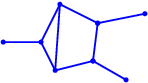
Example : Ring attached to a wire (figure 1).– If we consider for $\mathcal{G}_{1}$ a ring of perimeter $L$ pierced by a flux $\theta$ (corresponding to $A(x)=\theta/L$), we have : $S_{\mathrm{ring}}=2(\cosh\sqrt{\gamma}L-\cos\theta)$ and $S^{\mathrm{Dir}}_{\mathrm{ring}}=\frac{\sinh\sqrt{\gamma}L}{\sqrt{\gamma}}$. The graph $\mathcal{G}_{2}$ is a wire of length $b$ with Neumann boundary at its ends (for a vertex $\alpha$ of coordination number $m_{\alpha}=1$ the case $\lambda_{\alpha}=0$ coincides with Neumann boundary condition) : $S_{\mathrm{wire}}^{\mathrm{both\>Neu}}=\sqrt{\gamma}\sinh\sqrt{\gamma}b$ and $S_{\mathrm{wire}}^{\mathrm{Neu/Dir}}=\cosh\sqrt{\gamma}b$ . Therefore, we recover the simple result : $S(\gamma)=\sinh\sqrt{\gamma}b\,\sinh\sqrt{\gamma}L+2\cosh\sqrt{\gamma}b\,(\cosh\sqrt{\gamma}L-\cos\theta)$ obtained directly from (1) in Ref. [15].

Eq. (On the spectrum of the Laplace operator of metric graphs
attached at a vertex – Spectral determinant approach) is contained in eq. (9).– The result (9) has appeared as a limit of eq. (On the spectrum of the Laplace operator of metric graphs
attached at a vertex – Spectral determinant approach), therefore it seems at first sight a particular case of this latter equation. We show now that eq. (On the spectrum of the Laplace operator of metric graphs
attached at a vertex – Spectral determinant approach) can in fact be recovered from (9). For that purpose we proceed in two steps. First we attach a wire of length $b$ to the graph $\mathcal{G}_{1}$. The graph formed is denoted $\mathcal{G}_{\mathrm{inter}}$ and the corresponding spectral determinants $S_{\mathrm{inter}}$ and $S_{\mathrm{inter}}^{\mathrm{Dir}}$, depending on the nature of the boundary condition at the end of the wire. Spectral determinants of the wire for the three different boundary conditions, $S_{\mathrm{wire}}^{\mathrm{both\>Neu}}$, $S_{\mathrm{wire}}^{\mathrm{Neu/Dir}}$ and $S_{\mathrm{wire}}^{\mathrm{both\>Dir}}\equiv{S}^{\mathrm{Dir}}_{\mathrm{ring}}$, were given above. Therefore, from eq. (9) we obtain :

In a second step we attach the graph $\mathcal{G}_{2}$ to the end of the wire of $\mathcal{G}_{\mathrm{inter}}$. We use again eq. (9) from which it follows that $S_{\widetilde{\mathcal{G}}}=S_{\mathrm{inter}}S_{2}^{\mathrm{Dir}}+S_{\mathrm{inter}}^{\mathrm{Dir}}S_{2}$, that precisely coincides with eq. (On the spectrum of the Laplace operator of metric graphs
attached at a vertex – Spectral determinant approach).

Attachment of two graphs for Schrödinger operator.– Let us consider the spectral determinant for the Schrödinger operator (Hill operator) $S_{\mathcal{G}}(\gamma)=\det(\gamma-\Delta+V(x))$ with the same (continuous) boundary conditions as above. Let us first discuss how (1,2) are modified. $V_{\alpha\beta}(x_{\alpha\beta})$, with $x_{\alpha\beta}\in[0,l_{\alpha\beta}]$, is the component of the scalar potential $V(x)$ on the bond. An important ingredient is the solution $f_{\alpha\beta}(x_{\alpha\beta})$ of the differential equation $[\gamma-\frac{{\rm d}^{2}}{{\rm d}{x_{\alpha\beta}^{2}}}+V_{\alpha\beta}(x_{\alpha\beta})]f_{\alpha\beta}(x_{\alpha\beta})=0$ on the interval $[0,l_{\alpha\beta}]$, satisfying $f_{\alpha\beta}(0)=1$ and $f_{\alpha\beta}(l_{\alpha\beta})=0$. A second independent solution of the differential equation is $f_{\beta\alpha}(x_{\beta\alpha})=f_{\beta\alpha}(l_{\alpha\beta}-x_{\alpha\beta})$ (one should not make a confusion : despite we use the same notation, the $2B$ functions $f_{\alpha\beta}$ are not the $B$ components of a scalar function). If $V_{\alpha\beta}(x_{\alpha\beta})=0$ we have obviously $f_{\alpha\beta}(x)=\frac{\sinh\sqrt{\gamma}(l_{\alpha\beta}-x)}{\sinh\sqrt{\gamma}{}l_{\alpha\beta}}$. It was shown in Ref. [11]²² 2 The notations used here are slightly different from those of Ref. [11]. They coincide with those of Refs. [16, 8]. that eqs. (1,2) are generalized by performing the substitution $\sqrt{\gamma}\coth\sqrt{\gamma}l_{\alpha\beta}\to-f_{\alpha\beta}^{\prime}(0)$ and $\frac{\sqrt{\gamma}}{\sinh\sqrt{\gamma}l_{\alpha\beta}}\to-f_{\alpha\beta}^{\prime}(l_{\alpha\beta})$. The matrix $\mathcal{M}$ becomes $\mathcal{M}_{\alpha\beta}=\delta_{\alpha\beta}[\lambda_{\alpha}-\sum_{\mu}a_{\alpha\mu}f_{\alpha\mu}^{\prime}(0)]+a_{\alpha\beta}f_{\alpha\beta}^{\prime}(l_{\alpha\beta})\,{\mbox{\large e}}^{-{\rm i}\theta_{\alpha\beta}}$ and the spectral determinant takes the form³³ 3 The fact that $S_{\mathcal{G}}(\gamma)\propto\det\mathcal{M}$ has already been demonstrated in Ref. [17], however the remaining factor has been obtained in Ref. [11] by construction of the resolvent in the graph. Note that the Dirichlet determinant $[\prod_{({\alpha\beta})}f_{\alpha\beta}^{\prime}(l_{\alpha\beta})]^{-1}$ may play a role in order to determine the full spectrum. A trivial example is the wire (with $V(x)=0$) for which $\det\mathcal{M}=\gamma$, that does not determine the spectrum. Another example is studied in detail in section 12 of Ref. [7]. The $\gamma$-dependent factor $[\prod_{({\alpha\beta})}f_{\alpha\beta}^{\prime}(l_{\alpha\beta})]^{-1}$ is also important from a physical point of view since $\frac{\partial}{\partial\gamma}\ln{S(\gamma)}$ (for $V(x)=0$) has been shown to be related to several physical quantities [9, 7, 8]. $S_{\mathcal{G}}(\gamma)=[\prod_{({\alpha\beta})}f_{\alpha\beta}^{\prime}(l_{\alpha\beta})]^{-1}\det\mathcal{M}$.

Attachment of $n$ graphs.– We consider a graph $\mathcal{G}$ obtained by attachment of $n$ graphs at the same point (figure 2.d). It is now easy to generalize (9) in order to describe this situation. We start from (9) : $S_{\mathcal{G}}=S_{1}\,S^{\mathrm{Dir}}_{2+\cdots+n}+S^{\mathrm{Dir}}_{1}\,S_{2+\cdots+n}$ and use $S^{\mathrm{Dir}}_{2+\cdots+n}=S^{\mathrm{Dir}}_{2}\cdots{S}^{\mathrm{Dir}}_{n}$. Proceeding by recurrence, we end with :

Cayley tree.– We can use (12) to study the case of a Cayley tree of coordination number $z$. We denote $S_{n}$ the spectral determinant of a Cayley tree of depth $n$ with $\lambda_{\alpha}=0\hskip 8.5359pt\forall\,\alpha$. The spectral determinant for the similar graph with Dirichlet boundary at one of its end is denoted $S_{n}^{\mathrm{Dir}}$. We proceed in two steps represented on figure 3 : first we attach $z-1$ such trees together, using (12). Then we attach a wire of length $b$ by using (9). We find :

with $S_{1}=S_{\mathrm{wire}}^{\mathrm{both\>Neu}}$ and $S_{1}^{\mathrm{Dir}}=S_{\mathrm{wire}}^{\mathrm{Neu/Dir}}$. Note that in the case $z=2$ the recurrence is trivially solved and give the spectral determinants for a wire of length $nb$.

Conclusion.– Let us come back to the initial question of the paper. Eq. (9) seems at first sight to involve only spectral information on graphs $\mathcal{G}_{1}$, $\mathcal{G}_{2}$ and $\mathcal{G}$, however we mentioned above that, in eq. (1), the $\gamma$-independent prefactor is not a priori fixed by spectral information. Therefore we can only provide here a partial answer to the initial question : given the spectral determinants of two metric graphs $\mathcal{G}_{1}$ and $\mathcal{G}_{2}$, defined by (1), we can determine the spectrum of the graph $\mathcal{G}$ formed by attaching the two graphs at a vertex. An interesting development would be to provide a relation similar to (9) when the spectral determinant and its $\gamma$-independent prefactor are constructed from the spectrum only. In the case of $\zeta$-regularization of Ref. [14], the relation between $\zeta$-regularized determinant and (1), mentioned in a footnote above, suggests that the relation for $\zeta$-regularized determinants analogous to (9) also involves some information on the coordination numbers of vertices.

Acknowledgments.– I thank Y. Colin de Verdière and Alain Comtet for interesting discussions.

Appendix : derivative continous at the vertices.– The boundary conditions discussed in this article ($\varphi(x)$ continuous and $\sum_{\beta}{a}_{\alpha\beta}\varphi_{\alpha\beta}^{\prime}(0)=\lambda_{\alpha}\,\varphi_{\alpha}$) can be interpreted as the introduction of a $\delta$-potential at the vertex. They are denoted “$\delta$-coupling” in Ref. [17], where “$\delta^{\prime}$-coupling” are also introduced. These latter correspond to continuity of the derivative : $\varphi^{\prime}_{\alpha\beta}(0)=\varphi^{\prime}_{\alpha}\>\forall\>\beta$ neighbour of $\alpha$ and $\sum_{\beta}{a}_{\alpha\beta}\varphi_{\alpha\beta}(0)=\mu_{\alpha}\,\varphi^{\prime}_{\alpha}$ (the limit $\mu_{\alpha}\to\infty$ corresponds to Neumann boundary condition $\varphi^{\prime}_{\alpha}=0$). The results of the present article are easily generalized to the case of $\delta^{\prime}$-couplings.

Spectral determinant.– The spectral determinant now involves the solution of the differential equation $[\gamma-\frac{{\rm d}^{2}}{{\rm d}{x_{\alpha\beta}^{2}}}+V_{\alpha\beta}(x_{\alpha\beta})]g_{\alpha\beta}(x_{\alpha\beta})=0$ on the interval $[0,l_{\alpha\beta}]$, satisfying $g^{\prime}_{\alpha\beta}(0)=1$ and $g^{\prime}_{\alpha\beta}(l_{\alpha\beta})=0$. The spectral determinant is given by $S_{\mathcal{G}}(\gamma)=[\prod_{({\alpha\beta})}g_{\alpha\beta}(l_{\alpha\beta})]^{-1}\det\mathcal{N}$ with $\mathcal{N}_{\alpha\beta}=\delta_{\alpha\beta}[\mu_{\alpha}-\sum_{\nu}a_{\alpha\nu}g_{\alpha\nu}(0)]-a_{\alpha\beta}g_{\alpha\beta}(l_{\alpha\beta})\,{\mbox{\large e}}^{-{\rm i}\theta_{\alpha\beta}}$. Note that $[\prod_{({\alpha\beta})}g_{\alpha\beta}(l_{\alpha\beta})]^{-1}$ corresponds to the Neumann determinant : disconnected wires with Neumann boundary conditions $\mu_{\alpha}\to\infty\>\forall\>\alpha$). In the absence of a potential, $V(x)=0$ :

and $S_{\mathcal{G}}(\gamma)=(\prod_{({\alpha\beta})}\sqrt{\gamma}\sinh\sqrt{\gamma}l_{\alpha\beta})\>\det\mathcal{N}$.

Graph attachment.– We consider $n$ Graphs charaterized by spectral determinants $S_{k}$ for $k=1,\cdots,n$. We introduce the notation $S_{k}^{\mathrm{Neu}}=\lim_{\mu_{\alpha}\to\infty}\frac{S_{k}}{\mu_{\alpha}}$, where $\alpha$ is the vertex of attachment of the $n$ graphs (figure 2.d). Since spectral determinants for continuous boundary conditions and continuous derivative have similar structures, the results obtained in this article are easily generalized. In particular the result (12), from which other results have been derived, becomes for $\delta^{\prime}$-couplings

References

- [1] D. Burghelea, L. Friedlander, and T. Kappeler, Meyer-Vietoris type formula for determinants of elliptic differential operators, J. Funct. Anal. 107, 34 (1992).
- [2] V. Kostrykin and R. Schrader, Kirchhoff’s rule for quantum wires, J. Phys. A: Math. Gen. 32, 595 (1999).
- [3] N. I. Gerasimenko and B. S. Pavlov, Scattering problems on noncompact graphs, Theor. Math. Phys. 74, 230 (1988).
- [4] P. Exner and P. Šeba, Free quantum motion on a branching graph, Rep. Math. Phys. 28, 7 (1989).
- [5] V. Adamyan, Scattering matrices for microschemes, Oper. Theory: Adv. & Appl. 59, 1 (1992).
- [6] C. Texier and G. Montambaux, Scattering theory on graphs, J. Phys. A: Math. Gen. 34, 10307–10326 (2001).
- [7] E. Akkermans, A. Comtet, J. Desbois, G. Montambaux, and C. Texier, On the spectral determinant of quantum graphs, Ann. Phys. (N.Y.) 284, 10–51 (2000).
- [8] A. Comtet, J. Desbois, and C. Texier, Functionals of the Brownian motion, localization and metric graphs, J. Phys. A: Math. Gen. 38, R341–R383 (2005).
- [9] M. Pascaud and G. Montambaux, Persistent currents on networks, Phys. Rev. Lett. 82, 4512 (1999).
- [10] Y. Colin de Verdière, Déterminants et intégrales de Fresnel, Annales de l’Institut Fourier 49, 861 (1999).
- [11] J. Desbois, Spectral determinant of Schrödinger operators on graphs, J. Phys. A: Math. Gen. 33, L63 (2000).
- [12] J. Desbois, Spectral determinant on graphs with generalized boundary conditions, Eur. Phys. J. B 24, 261 (2001).
- [13] R. Forman, Functional determinants and geometry, Invent. math. 88, 447 (1987).
- [14] L. Friedlander, Determinant of the Schrödinger operator on a metric graph, Contemporary Mathematics 415, 151 (2006).
- [15] C. Texier and G. Montambaux, Quantum oscillations in mesoscopic rings and anomalous diffusion, J. Phys. A: Math. Gen. 38, 3455–3471 (2005).
- [16] C. Texier and P. Degiovanni, Charge and current distribution in graphs, J. Phys. A: Math. Gen. 36, 12425–12452 (2003).
- [17] P. Exner, A duality between Schrödinger operators on graphs and certain Jacobi matrices, Ann. Inst. H. Poincaré : Phys. Théor. 66, 359 (1997).
- [18] J. E. Avron and L. Sadun, Adiabatic quantum transport in networks with macroscopic components, Ann. Phys. (N.Y.) 206, 440 (1991).
- [19] V. Kostrykin and R. Schrader, The generalized star product and the factorization of scattering matrices on graphs, J. Math. Phys. 42, 1563 (2001).