¹¹ 1 Supported in part at the Technion by a fellowship of the Israel Council for Higher Education

Reading Off Kurosh Decompositions

L.Markus-Epstein Address: Department of Mathematics
Technion
Haifa 32000, Israel Email address: epstin@math.biu.ac.il

Abstract.

Geometric methods proposed by Stallings [18] for treating finitely generated subgroups of free groups were successfully used to solve a wide collection of decision problems for free groups and their subgroups [2, 7, 11, 12, 16, 17, 21].

In the present paper we employ the generalized Stallings’ folding method developed in [13] to introduce a procedure, which given a subgroup $H$ of a free product of finite groups reads off its Kurosh decomposition from the subgroup graph of $H$ .

1. Introduction

The celebrated theorem of Kurosh describes subgroups of free products.

Theorem 1.1 (Kurosh Subgroup Theorem [10]).

Let $G$ be a free product of groups $G_{i}$ , where $i$ runs over an index set $I$ . Let $H$ be a subgroup of $G$ . Then $H=F\ast(\ast g_{j}H_{j}g_{j}^{-1})$ is a free product of a free group $F$ together with groups that are conjugates of subgroups $H_{j}$ of the free factors $G_{i}$ of $G$ .

In this issue one can ask the following algorithmic question. Given a subgroup $H$ (for instance, by a finite set of generators) of a free product $G=\ast G_{i}$ , find its Kurosh decomposition $H=F\ast(\ast g_{j}H_{j}g_{j}^{-1})$ efficiently.

Below we solve this algorithmic problem (we call it the Kurosh decomposition problem) for finitely generated subgroups of free products of finite groups, employing graph theoretical methods developed by the author in [13]. More precisely, we introduce an algorithm which reads off the decomposition of a subgroup from its subgroup graph.

This approach goes back to the remarkable paper of Stallings [18], where finitely generated subgroups of free groups were canonically represented by finite labelled graphs. Later on this method was successfully applied to solve various algorithmic problems in free groups [2, 7, 11, 12, 16, 17, 21], providing mostly polynomial algorithms.

In [13] Stallings method, or so called Stallings’ folding algorithm, was generalized to the class of amalgams of finite groups. We refer to this generalized algorithm as the generalized Stallings’ folding algorithm. In the current paper our methods are restricted to the case of free products of finite groups. The description of the generalized Stallings’ algorithm (restricted to the case of free products of finite groups) is included in the Appendix.

Note that the graph constructed by Stallings’ folding algorithm for $S\leq FG(X)$ is the Geodesic core of the coset Cayley graph of $FG(X)$ relative to $S$ , that is the the union of all closed geodesic paths starting at the basepoint $S\cdot 1$ . The resulting graph $(\Gamma(H),v_{0})$ constructed by the generalized Stallings’ folding algorithm for $H\leq G$ is a sort of a core graph as well (see [13] for more details). More precisely, it is the Normal core of the coset Cayley graph of $G$ relative to $H$ : the union of all closed normal paths starting at the basepoint $H\cdot 1$ . Another example of core construction can be found in [4], where Collins and Turner use a topological approach to study automorphisms of free products.

The paper is organized as follows. We start (Section 3) by fixing the notation and by brief recalling of some known results which are essential for the current paper. Readers familiar with free products, normal (reduced) words and labelled graphs can skip it. The next section (Section 4) presents a summary of the results from [13] concerning subgroup graphs which are essential for the solution of Kurosh decomposition problem.

Section 5 presents the basic step of our “reading” procedure described along with the proof of Theorem 6.4 (Section 6). The complexity analysis of this algorithm shows that it is quadratic in the size of the input. The algorithm application is demonstrated in Example 3 (Section 6).

2. Acknowledgments

I wish to deeply thank to my PhD advisor Prof. Stuart W. Margolis for introducing me to this subject, for his help and encouragement throughout my work on the thesis. I owe gratitude to Prof. Arye Juhasz for his suggestions and many useful comments during the writing of this paper. I gratefully acknowledge a partial support at the Technion by a fellowship of the Israel Council for Higher Education.

3. Preliminaries

Free Products

Throughout this paper, we assume that $G=G_{1}\ast G_{2}$ is a free product of finite groups $G_{1}$ and $G_{2}$ where

(

\ast

)

\displaystyle G_{1}=gp\langle X_{1}|R_{1}\rangle,\ \ G_{2}=gp\langle X_{2}|R_{2}\rangle\ \ {\rm such\ that}\ \ X_{1}^{\pm}\cap X_{2}^{\pm}=\emptyset.

Thus

(

\ast\ast

)

\displaystyle{G=gp\langle X_{1},X_{2}|R_{1},R_{2}\rangle.}

We denote $X=X_{1}\cup X_{2}$ and put $H$ to be a finitely generated subgroup of $G$ .

Elements of $G=gp\langle X|R\rangle$ are equivalence classes of words. However it is customary to blur the distinction between a word $u$ and the equivalence class containing $u$ . We will distinguish between them by using different equality signs: “ $\equiv$ ” for the equality of two words and “ $=_{G}$ ” to denote the equality of two elements of $G$ , that is the equality of two equivalence classes.

Normal Forms

Let $G=G_{1}\ast_{A}G_{2}$ .

A word $g_{1}g_{2}\cdots g_{n}\in G$ ( $n\geq 0$ ) is in normal form (or, more customary, it is a normal word) if the following holds

(1)

$g_{i}\neq_{G}1$ lies in either $G_{1}$ or $G_{2}$ ,
(2)

$g_{i}$ and $g_{i+1}$ are in different factors of $G$ ,

We call the sequence $(g_{1},g_{2},\ldots,g_{n})$ a normal decomposition of the element $g\in G$ , where $g=_{G}g_{1}g_{2}\cdots g_{n}$ .

By the Normal Form Theorem for Free Products (Theorem IV.1.2 in [10]), the number $n$ is uniquely determined for a given element $g$ of $G$ and it is called the syllable length of $g$ .

Labelled graphs

Below we follow the notation of [5, 18].

A graph $\Gamma$ consists of two sets $E(\Gamma)$ and $V(\Gamma)$ , and two functions $E(\Gamma)\rightarrow E(\Gamma)$ and $E(\Gamma)\rightarrow V(\Gamma)$ : for each $e\in E$ there is an element $\overline{e}\in E(\Gamma)$ and an element $\iota(e)\in V(\Gamma)$ , such that $\overline{\overline{e}}=e$ and $\overline{e}\neq e$ .

The elements of $E(\Gamma)$ are called edges, and an $e\in E(\Gamma)$ is a direct edge of $\Gamma$ , $\overline{e}$ is the reverse (inverse) edge of $e$ .

The elements of $V(\Gamma)$ are called vertices, $\iota(e)$ is the initial vertex of $e$ , and $\tau(e)=\iota(\overline{e})$ is the terminal vertex of $e$ . We call them the endpoints of the edge $e$ .

A path of length $n$ is a sequence of $n$ edges $p=e_{1}\cdots e_{n}$ such that $v_{i}=\tau(e_{i})=\iota(e_{i+1})$ ( $1\leq i<n$ ). We call $p$ a path from $v_{0}=\iota(e_{1})$ to $v_{n}=\tau(e_{n})$ . The inverse of the path $p$ is $\overline{p}=\overline{e_{n}}\cdots\overline{e_{1}}$ . A path of length 0 is the empty path.

We say that the graph $\Gamma$ is connected if $V(\Gamma)\neq\emptyset$ and any two vertices are joined by a path. The path $p$ is closed if $\iota(p)=\tau(p)$ , and it is freely reduced if $e_{i+1}\neq\overline{e_{i}}$ ( $1\leq i<n$ ). $\Gamma$ is a tree if it is a connected graph and every closed freely reduced path in $\Gamma$ is empty.

A subgraph of $\Gamma$ is a graph $C$ such that $V(C)\subseteq V(\Gamma)$ and $E(C)\subseteq E(\Gamma)$ . In this case, by abuse of language, we write $C\subseteq\Gamma$ . Similarly, whenever we write $\Gamma_{1}\cup\Gamma_{2}$ or $\Gamma_{1}\cap\Gamma_{2}$ , we always mean that the set operations are, in fact, applied to the vertex sets and the edge sets of the corresponding graphs.

A labelling of $\Gamma$ by the set $X^{\pm}$ is a function

lab:\>E(\Gamma)\rightarrow X^{\pm}

such that for each $e\in E(\Gamma)$ , $lab(\overline{e})\equiv(lab(e))^{-1}$ .

The last equality enables one, when representing the labelled graph $\Gamma$ as a directed diagram, to represent only $X$ -labelled edges, because $X^{-1}$ -labelled edges can be deduced immediately from them.

A graph with a labelling function is called a labelled (with $X^{\pm}$ ) graph. The only graphs considered in the present paper are labelled graphs.

A labelled graph is called well-labelled if

\iota(e_{1})=\iota(e_{2}),\;lab(e_{1})\equiv lab(e_{2})\ \Rightarrow\ e_{1}=e_{2},

for each pair of edges $e_{1},e_{2}\in E(\Gamma)$ . See Figure 1.

Refer to caption — Figure 1. The graph $\Gamma_{1}$ is labelled with $\{a,b,c\}^{\pm}$ , but it is not well-labelled. The graphs $\Gamma_{2}$ and $\Gamma_{3}$ are well-labelled with $\{a,b,c\}^{\pm}$ .

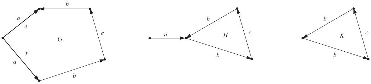
If a finite graph $\Gamma$ is not well-labelled then a process of iterative identifications of each pair $\{e_{1},e_{2}\}$ of distinct edges with the same initial vertex and the same label to a single edge yields a well-labelled graph. Such identifications are called foldings, and the whole process is known as the process of Stallings’ foldings [2, 7, 11, 12]. Thus the graph $\Gamma_{2}$ on Figure 1 is obtained from the graph $\Gamma_{1}$ by folding the edges $e_{1}$ and $e_{2}$ to a single edge labelled by $a$ .

Notice that the graph $\Gamma_{3}$ is obtained from the graph $\Gamma_{2}$ by removing the edge labelled by $a$ whose initial vertex has degree 1. Such an edge is called a hair, and the above procedure is used to be called “cutting hairs”.

The label of a path $p=e_{1}e_{2}\cdots e_{n}$ in $\Gamma$ , where $e_{i}\in E(\Gamma)$ , is the word

lab(p)\equiv lab(e_{1})\cdots lab(e_{n})\in(X^{\pm})^{*}.

Notice that the label of the empty path is the empty word. As usual, we identify the word $lab(p)$ with the corresponding element in $G=gp\langle X|R\rangle$ . We say that $p$ is a normal path (or $p$ is a path in normal form) if $lab(p)$ is a normal word.

If $\Gamma$ is a well-labelled graph then a path $p$ in $\Gamma$ is freely reduced if and only if $lab(p)$ is a freely reduced word. Otherwise $p$ can be converted into a freely reduced path $p^{\prime}$ by iteratively removing of the subpaths $e\overline{e}$ (backtrackings) ([11, 7]). Thus

\iota(p^{\prime})=\iota(p),\ \tau(p^{\prime})=\tau(p)\ \;{\rm and}\ \;lab(p)=_{FG(X)}lab(p^{\prime}),

where $FG(X)$ is a free group with a free basis $X$ . We say that $p^{\prime}$ is obtained from $p$ by free reductions.

If $v_{1},v_{2}\in V(\Gamma)$ and $p$ is a path in $\Gamma$ such that

\iota(p)=v_{1},\ \tau(p)=v_{2}\ {\rm and}\ lab(p)\equiv u,

then, following the automata theoretic notation, we simply write $v_{1}\cdot u=v_{2}$ to summarize this situation, and say that the word $u$ is readable at $v_{1}$ in $\Gamma$ .

A pair $(\Gamma,v_{0})$ consisting of the graph $\Gamma$ and the basepoint $v_{0}$ (a distinguished vertex of the graph $\Gamma$ ) is called a pointed graph.

Following the notation of Gitik ([5]) we denote the set of all closed paths in $\Gamma$ starting at $v_{0}$ by $Loop(\Gamma,v_{0})$ , and the image of $lab(Loop(\Gamma,v_{0}))$ in $G=gp\langle X|R\rangle$ by $Lab(\Gamma,v_{0})$ . More precisely,

Loop(\Gamma,v_{0})=\{p\;|\;p{\rm\ is\ a\ path\ in\ \Gamma\ with}\ \iota(p)=\tau(p)=v_{0}\},

Lab(\Gamma,v_{0})=\{g\in G\;|\;\exists p\in Loop(\Gamma,v_{0})\;:\;lab(p)=_{G}g\}.

It is easy to see that $Lab(\Gamma,v_{0})$ is a subgroup of $G$ ([5]). Moreover, $Lab(\Gamma,v)=gLab(\Gamma,u)g^{-1}$ , where $g=_{G}lab(p)$ , and $p$ is a path in $\Gamma$ from $v$ to $u$ ([7]). If $V(\Gamma)=\{v_{0}\}$ and $E(\Gamma)=\emptyset$ then we assume that $H=\{1\}$ .

We say that $H=Lab(\Gamma,v_{0})$ is the subgroup of $G$ determined by the graph $(\Gamma,v_{0})$ . Thus any pointed graph labelled by $X^{\pm}$ , where $X$ is a generating set of a group $G$ , determines a subgroup of $G$ . This argues the use of the name subgroup graphs for such graphs.

Morphisms of Labelled Graphs

Let $\Gamma$ and $\Delta$ be graphs labelled with $X^{\pm}$ . The map $\pi:\Gamma\rightarrow\Delta$ is called a morphism of labelled graphs, if $\pi$ takes vertices to vertices, edges to edges, preserves labels of direct edges and has the property that

\iota(\pi(e))=\pi(\iota(e))\ {\rm and}\ \tau(\pi(e))=\pi(\tau(e)),\ \forall e\in E(\Gamma).

An injective morphism of labelled graphs is called an embedding. If $\pi$ is an embedding then we say that the graph $\Gamma$ embeds in the graph $\Delta$ .

A morphism of pointed labelled graphs $\pi:(\Gamma_{1},v_{1})\rightarrow(\Gamma_{2},v_{2})$ is a morphism of underlying labelled graphs $\pi:\Gamma_{1}\rightarrow\Gamma_{2}$ which preserves the basepoint $\pi(v_{1})=v_{2}$ . If $\Gamma_{2}$ is well-labelled then there exists at most one such morphism ([7]).

Remark 3.1 ([7]).

If two pointed well-labelled (with $X^{\pm}$ ) graphs $(\Gamma_{1},v_{1})$ and $(\Gamma_{2},v_{2})$ are isomorphic, then there exists a unique isomorphism $\pi:(\Gamma_{1},v_{1})\rightarrow(\Gamma_{2},v_{2})$ . Therefore $(\Gamma_{1},v_{1})$ and $(\Gamma_{2},v_{2})$ can be identified via $\pi$ . In this case we sometimes write $(\Gamma_{1},v_{1})=(\Gamma_{2},v_{2})$ . $\diamond$

The notation $\Gamma_{1}=\Gamma_{2}$ means that there exists an isomorphism between these two graphs. More precisely, one can find $v_{i}\in V(\Gamma_{i})$ ( $i\in\{1,2\}$ ) such that $(\Gamma_{1},v_{1})=(\Gamma_{2},v_{2})$ in the sense of Remark 3.1.

4. Subgroup Graphs

The current section is devoted to the discussion on subgroup graphs constructed by the generalized Stallings’ folding algorithm. The main results of [13] concerning these graphs, which are essential for the present paper, are summarized in terms of free products in Theorem 4.1 below. The notion of reduced precover is explained right after the theorem along the rest of this section.

Theorem 4.1.

Let $H=\langle h_{1},\cdots,h_{k}\rangle$ be a finitely generated subgroup of a free product of finite groups $G=G_{1}\ast G_{2}$ .

Then there is an algorithm (the generalized Stallings’ folding algorithm) which constructs a finite labelled graph $(\Gamma(H),v_{0})$ with the following properties:

(1)

${Lab(\Gamma(H),v_{0})}={H}.$
(2)

Up to isomorphism, $(\Gamma(H),v_{0})$ is a unique reduced precover of $G$ determining $H$ .
(3)

Let $m$ be the sum of the lengths of words $h_{1},\ldots h_{n}$ . Then the algorithm computes $(\Gamma(H),v_{0})$ in time $O(m^{2})$ . Moreover, $|V(\Gamma(H))|$ and $|E(\Gamma(H))|$ are proportional to $m$ .

Throughout the present paper the notation $(\Gamma(H),v_{0})$ is always used for the finite labelled graph constructed by the generalized Stallings’ folding algorithm for a finitely generated subgroup $H$ of a free product of finite groups $G=G_{1}\ast G_{2}$ .

Precovers

Roughly speaking, precovers are subgroup graphs, corresponding to subgroups of amalgamated products, with a very particular structure. This notion was defined by Gitik in [5] and actively employed by the author in [13, 14, 15]. Below we define precovers in term of free products and recall some of their properties which are essential to the present paper.

Let $\Gamma$ be a graph well-labelled with $X^{\pm}$ , where $X=X_{1}\cup X_{2}$ is the generating set of $G=G_{1}\ast G_{2}$ given by ( $\ast$ ) and ( $\ast\ast$ ). We view $\Gamma$ as a two colored graph: one color for each one of the generating sets $X_{1}$ and $X_{2}$ of the factors $G_{1}$ and $G_{2}$ , respectively.

The vertex $v\in V(\Gamma)$ is called $X_{i}$ -monochromatic if all the edges of $\Gamma$ incident with $v$ are labelled with $X_{i}^{\pm}$ , for some $i\in\{1,2\}$ . We denote the set of $X_{i}$ -monochromatic vertices of $\Gamma$ by $VM_{i}(\Gamma)$ and put $VM(\Gamma)=VM_{1}(\Gamma)\cup VM_{2}(\Gamma)$ .

We say that a vertex $v\in V(\Gamma)$ is bichromatic if there exist edges $e_{1}$ and $e_{2}$ in $\Gamma$ with

\iota(e_{1})=\iota(e_{2})=v\ {\rm and}\ lab(e_{i})\in X_{i}^{\pm},\ i\in\{1,2\}.

The set of bichromatic vertices of $\Gamma$ is denoted by $VB(\Gamma)$ .

A subgraph of $\Gamma$ is called monochromatic if it is labelled only with $X_{1}^{\pm}$ or only with $X_{2}^{\pm}$ . An $X_{i}$ -monochromatic component of $\Gamma$ ( $i\in\{1,2\}$ ) is a maximal connected subgraph of $\Gamma$ labelled with $X_{i}^{\pm}$ , which contains at least one edge. Thus monochromatic components of $\Gamma$ are graphs determining subgroups of the factors, $G_{1}$ or $G_{2}$ .

We say that a graph $\Gamma$ is $G$ -based if any path $p\subseteq\Gamma$ with $lab(p)=_{G}1$ is closed. Thus if $\Gamma$ is $G$ -based then, obviously, it is well-labelled with $X^{\pm}$ .

Definition 4.2 (Definition of Precover).

A $G$ -based graph $\Gamma$ is a precover of $G=G_{1}\ast G_{2}$ if each $X_{i}$ -monochromatic component of $\Gamma$ is a cover of $G_{i}$ ( $i\in\{1,2\}$ ).

Following the terminology of Gitik ([5]), we use the term “covers of $G$ ” for relative (coset) Cayley graphs of $G$ and denote by $Cayley(G,S)$ the coset Cayley graph of $G$ relative to the subgroup $S$ of $G$ .²² 2 Whenever the notation $Cayley(G,S)$ is used, it always means that $S$ is a subgroup of the group $G$ and the presentation of $G$ is fixed and clear from the context. If $S=\{1\}$ , then $Cayley(G,S)$ is the Cayley graph of $G$ and the notation $Cayley(G)$ is used.

Note that the use of the term “covers” is adjusted by the well known fact that a geometric realization of a coset Cayley graph of $G$ relative to some $S\leq G$ is a 1-skeleton of a topological cover corresponding to $S$ of the standard 2-complex representing the group $G$ (see [19], pp.162-163).

Remark 4.3.

Recall that $G=G_{1}\ast G_{2}=gp\langle X|R\rangle$ is given by $(\ast)$ and $(\ast\ast)$ .

Let $\Gamma$ be a graph well-labelled with $X^{\pm}$ such that each $X_{i}$ -monochromatic component of $\Gamma$ is a cover of $G_{i}$ ( $i\in\{1,2\}$ ). Hence $\Gamma$ is $G$ -based, because each cover of $G_{i}$ is a $G_{i}$ -based graph.

This allows one to simplify the definition of precovers in the case of free products by saying that a graph $\Gamma$ is a precover of $G=G_{1}\ast G_{2}$ if each $X_{i}$ -monochromatic component of $\Gamma$ is a cover of $G_{i}$ ( $i\in\{1,2\}$ ).

$\diamond$

Convention 4.4.

By the above definition, a precover doesn’t have to be a connected graph. However along this paper we restrict our attention only to connected precovers. Thus any time this term is used, we always mean that the corresponding graph is connected unless it is stated otherwise.

We follow the convention that a graph $\Gamma$ with $V(\Gamma)=\{v\}$ and $E(\Gamma)=\emptyset$ determining the trivial subgroup (that is $Lab(\Gamma,v)=\{1\}$ ) is a (an empty) precover of $G$ . $\diamond$

Example 4.5.

Let $G=\mathbb{Z}_{4}\ast\mathbb{Z}_{6}=gp\langle x,y|x^{4},y^{6}\rangle$ .

The graph $\Gamma_{1}$ on Figure 2 is an example of a precover of $G$ with one monochromatic component. $\Gamma_{2}$ , $\Gamma_{4}$ are examples of precovers of $G$ with two monochromatic components.

The graph $\Gamma_{3}$ is not a precover of $G$ because its $\{x\}$ -monochromatic components are not covers of $\mathbb{Z}_{4}$ . $\diamond$

A graph $\Gamma$ is $x$ -saturated at $v\in V(\Gamma)$ , if there exists $e\in E(\Gamma)$ with $\iota(e)=v$ and $lab(e)=x$ ( $x\in X$ ). $\Gamma$ is $X^{\pm}$ -saturated if it is $x$ -saturated for each $x\in X^{\pm}$ at each $v\in V(\Gamma)$ .

Lemma 4.6 (Lemma 1.5 in [5]).

Let $G=gp\langle X|R\rangle$ be a group and let $(\Gamma,v_{0})$ be a graph well-labelled with $X^{\pm}$ . Denote $Lab(\Gamma,v_{0})=S$ . Then

•

$\Gamma$ is $G$ -based if and only if it can be embedded in $(Cayley(G,S),S~\cdot~1)$ ,
•

$\Gamma$ is $G$ -based and $X^{\pm}$ -saturated if and only if it is isomorphic to $(Cayley(G,S),S\cdot~1)$ . ³³ 3 We write $S\cdot 1$ instead of the usual $S1=S$ to distinguish this vertex of $Cayley(G,S)$ as the basepoint of the graph.

Corollary 4.7.

If $\Gamma$ is a precover of $G$ with $Lab(\Gamma,v_{0})=H\leq G$ then $\Gamma$ is a subgraph of $Cayley(G,H)$ .

Thus a precover of $G$ can be viewed as a part of the corresponding cover of $G$ , which explains the use of the term “precovers”.

Definition 4.8 (Definition of Reduced Precover).

A reduced precover of $G$ is a precover $(\Gamma,v_{0})$ of $G$ with no redundant monochromatic components.

A $X_{i}$ -monochromatic component $C$ of the precover $(\Gamma,v_{0})$ is redundant if the following holds

•

$Lab(C,v)=\{1\}$ (equivalently, by Lemma 4.6, $C=Cayley(G_{i})$ ),
•

$|VB(C)|\leq 1$ ,
•

$v_{0}\not\in VM(C)$ .

Example 4.9.

Let $G=\mathbb{Z}_{4}\ast\mathbb{Z}_{6}=gp\langle x,y|x^{4},y^{6}\rangle$ .

Any choice of a basepoint in the graph $\Gamma_{1}$ on Figure 2 yields a non reduced precover, while any basepoint of $\Gamma_{4}$ gives a reduced precover.

In the graph $\Gamma_{2}$ any choice of the basepoint $v$ except that of $w$ (that is $v=w$ ) makes $(\Gamma_{2},v)$ to be a reduced precover of $G$ . $\diamond$

Remark 4.10 ([13]).

Let $\phi:\Gamma\rightarrow\Delta$ be a morphism of labelled graphs. If $\Gamma$ is a precover of $G$ , then $\phi(\Gamma)$ is a precover of $G$ as well. $\diamond$

5. The Basic Step

Let $G=G_{1}\ast G_{2}$ be a free product of finite groups given by $(\ast)$ and $(\ast\ast)$ .

Let $(\Gamma,v_{0})$ is a finite pointed $G$ -based graph with $Lab(\Gamma,v_{0})=H\leq G$ .

Let $C$ be a $X_{i}$ -monochromatic component of $\Gamma$ which is a cover of $G_{i}$ ( $i\in\{1,2\}$ ). Let $v\in V(C)$ be the basepoint of $C$ . Let $T(C)$ be a spanning tree of $C$ with the root vertex $v$ .

Let $P_{v}$ be an approach path in $\Gamma$ from the basepoint $v_{0}$ to a vertex $v\in V(C)$ (we assume that $P_{v}$ is freely reduced). We put $g_{v}\equiv lab(P_{v})$ .

Let $P_{v}=P_{v1}\cdots P_{vm}$ be a decomposition of $P_{v}$ into maximal monochromatic paths. Without loss of generality, we can assume that $P_{vm}\cap C=\{v\}$ . Otherwise, we choose the basepoint of $C$ to be $v^{\prime}=\tau(P_{v(m-1)})=\iota(P_{vm})$ and take the approach path $P_{v^{\prime}}$ to be $P_{v^{\prime}}=P_{v1}\cdots P_{v(m-1)}$ .

Following the above assumption, whenever $v_{0}\in V(C)$ we chose $v=v_{0}$ . Thus the path $P_{v}$ is empty and $g_{v}=_{G}1$ .

Let $\Gamma^{\prime}$ be the graph obtained from $\Gamma$ by removing all the edges of $C$ which are not in $E(T(C))$ . More precisely,

E(\Gamma^{\prime})=E(\Gamma)\setminus E(T(C)),\ \ V(\Gamma^{\prime})=V(\Gamma).

Evidently, the graph $\Gamma^{\prime}$ is connected. Roughly speaking, it is a subgraph of $\Gamma$ with $v_{0}\in V(\Gamma^{\prime})$ . Hence $(\Gamma^{\prime},v_{0})$ is a finite pointed $G$ -based graph. Moreover,

(1)

\Gamma^{\prime}\cap C=T(C)

Thus

(2)

Loop(C,v)\cap Loop(\Gamma^{\prime},v)=\emptyset.

To exploit the connection between $Lab(\Gamma,v_{0})$ , $Lab(C,v)$ and $Lab(\Gamma^{\prime},v_{0})$ we need the following classical result.

Lemma 5.1 (Lemma IV.1.7 [10]).

Let $A$ , $B$ be subgroups of a group $G$ such that $A\cup B$ generates $G$ , $A\cap B=\{1\}$ , and if $g_{1},\ldots,g_{n}$ is a reduced sequence with $n>0$ (that is each $g_{i}$ is in one of $A$ or $B$ and successive $g_{i}$ , $g_{i+1}$ are not in the same factor), then $g_{1}g_{2}\ldots g_{n}\neq_{G}1$ . Then $G\simeq A\ast B$ .

Now we are ready to give the desired connection. The following lemma is stated in terms of the above notation.

Lemma 5.2.

The following holds.

(i)

$H=\langle g_{v}Lab(C,v)g_{v}^{-1},Lab(\Gamma^{\prime},v_{0})\rangle.$
(ii)

$\langle g_{v}Lab(C,v)g_{v}^{-1},Lab(\Gamma^{\prime},v_{0})\rangle=g_{v}Lab(C,v_{r})g_{v}^{-1}\ast Lab(\Gamma^{\prime},v_{0}).$
(iii)

$H=g_{v}Lab(C,v)g_{v}^{-1}\ast Lab(\Gamma^{\prime},v_{0}).$

Proof.

(i)

Since $Lab(P_{v}Loop(C,v)\overline{P_{v}})=_{G}g_{v}Lab(C,v)g_{v}^{-1}$ and

P_{v}Loop(C,v)\overline{P_{v}}\subseteq Loop(\Gamma,v_{0}),

we have $g_{v}Lab(C,v)g_{v}^{-1}\leq H$ .

On the other hand, $(\Gamma^{\prime},v_{0})$ embeds in $(\Gamma,v_{0})$ . Hence $Lab(\Gamma^{\prime},v_{0})\leq Lab(\Gamma,v_{0})=H$ . Therefore

(3)

\langle g_{v}Lab(C,v)g_{v}^{-1},Lab(\Gamma^{\prime},v_{0})\rangle\subseteq H.

Conversely, let $h\in H$ . Thus there exists a path $q$ in $\Gamma$ such that $\iota(q)=\tau(q)=v_{0}$ and $lab(q)=_{G}h$ .

If $q$ is a path in $\Gamma^{\prime}$ or in $P_{v}Loop(C,v)\overline{P_{v}}$ . Then we are done.

Otherwise, there is a decomposition $q=q_{1}t_{1}q_{2}t_{2}\cdots t_{k-1}q_{k}$ , where $q_{i}$ are paths in $\Gamma^{\prime}$ and $t_{i}$ are paths in $C$ such that $t_{i}\cap\Gamma^{\prime}=\{\iota(t_{i}),\tau(t_{i})\}$ .

The path $t_{i}$ can be obtained by the path free reductions from the path

\overline{P_{v}p_{\iota(t_{i})}}P_{v}p_{\iota(t_{i})}t_{i}\overline{P_{v}p_{\tau(t_{i})}}P_{v}p_{\tau(t_{i})},

where $p_{\iota(t_{i})}$ and $p_{\tau(t_{i})}$ are the approach paths in the spanning tree $T(C)$ from the root vertex $v$ to the vertices $\iota(t_{i})$ and $\tau(t_{i})$ , respectively. Note that if $\iota(t_{i})=v$ or $\tau(t_{i})=v$ then the path $p_{\iota(t_{i})}$ or the path $p_{\tau(t_{i})}$ , respectively, is empty.

Thus the path $q_{i}t_{i}q_{i+1}$ can be obtained by the path free reductions from the path

(q_{i}\overline{P_{v}p_{\iota(t_{i})}})(P_{v}p_{\iota(t_{i})}t_{i}\overline{P_{v}p_{\tau(t_{i})}})(P_{v}p_{\tau(t_{i})}q_{i+1}).

The path $p_{\iota(t_{i})}t_{i}\overline{p_{\tau(t_{i})}}$ is in $C$ and it is closed at $v$ . Hence the path $P_{v}p_{\iota(t_{i})}t_{i}\overline{P_{v}p_{\tau(t_{i})}}$ is a path closed at $v_{0}$ in $\Gamma$ with $lab(P_{v}p_{\iota(t_{i})}t_{i}\overline{P_{v}p_{\tau(t_{i})}})\in g_{v}Lab(C,v)g_{v}^{-1}$ .

By the construction, the approach paths $P_{v}$ , $p_{\iota(t_{i})}$ are in $\Gamma^{\prime}$ . Thus the paths

q_{1}\overline{P_{v}p_{\iota(t_{1})}},\ \ P_{v}p_{\tau(t_{k-1})}q_{k}\ \ {\rm and}\ \ P_{v}p_{\tau(t_{i-1})}q_{i}\overline{P_{v}p_{\iota(t_{i})}}\ \ (\forall\>2\leq i\leq k-1)

are closed at $v_{0}$ in $\Gamma^{\prime}$ . Hence the labels of these paths are in $Lab(\Gamma^{\prime},v_{0})$ . Therefore

h\equiv lab(q)\in\langle g_{v}Lab(C,v)g_{v}^{-1},Lab(\Gamma^{\prime},v_{0})\rangle.

Thus

(4)

H\subseteq\langle g_{v}Lab(C,v)g_{v}^{-1},Lab(\Gamma^{\prime},v_{0})\rangle.

The combination of (3) and (4) gives the desired conclusion that

H=\langle g_{v}Lab(C,v)g_{v}^{-1},Lab(\Gamma^{\prime},v_{0})\rangle.

(ii) We assume that $Lab(C,v)\neq\{1\}$ , otherwise the statement is trivial. To get the desired equality we have to show that the conditions of Lemma 5.1 are satisfied.

Since $Lab(P_{v}Loop(C,v)\overline{P_{v}})=_{G}g_{v}Lab(C,v)g_{v}^{-1}$ and, by (2),

P_{v}Loop(C,v)\overline{P_{v}}\cap Loop(\Gamma^{\prime},v_{0})=\emptyset,

we have $g_{v}Lab(C,v)g_{v}^{-1}\cap Lab(\Gamma^{\prime},v_{0})=\{1\}$ .

To prove the satisfaction of the second condition of Lemma 5.1 we let

1\neq z_{l}\in g_{v}Lab(C,v)g_{v}^{-1}\ \ {\rm and}\ \ 1\neq w_{l}\in Lab(\Gamma^{\prime},v_{0})\ \ (1<l<k)

and show that

z_{1}w_{1}\cdots z_{k}w_{k}\neq_{G}1.

Hence there exist closed paths $t_{l}\in P_{v}Loop(C,v)\overline{P_{v}}$ and $s_{l}\in Loop(\Gamma^{\prime},v_{0})$ ( $1\leq l\leq k$ ) such that

lab(t_{l})=_{G}z_{l}\ \ {\rm and}\ \ lab(s_{l})=_{G}w_{l}.

Thus $lab(t_{l})=_{G}g_{v}z_{l}^{\prime}g_{v}^{-1}$ and there exists a nonempty path $t_{l}^{\prime}\in Loop(C,v)$ such that $1\neq z_{l}^{\prime}\equiv lab(t^{\prime}_{l})$ ( $1\leq l\leq k$ ). Hence $lab(t^{\prime}_{l})\in G_{i}$ is a normal word in $G$ of the syllable length 1.

On the other hand, $Lab(\Gamma^{\prime},v_{0})=g_{v}Lab(\Gamma^{\prime},v)g_{v}^{-1}$ . Hence, for all $1\leq l\leq k$ , there exists a nonempty path $s^{\prime}_{l}\in Loop(\Gamma^{\prime},v)$ such that

lab(s_{l})=_{G}g_{v}lab(s^{\prime}_{l})g_{v}^{-1}\ \ (lab(s^{\prime}_{l})\neq 1).

Since the graph $\Gamma^{\prime}$ is $G$ -based, we can assume (without loss of generality) that the path $s_{l}^{\prime}$ is normal, that is there is a decomposition of $s_{l}^{\prime}$ into maximal monochromatic paths $s_{l}^{\prime}=s^{\prime}_{l1}s^{\prime}_{l2}\cdots s^{\prime}_{lm_{l}}$ such that $lab(s_{lf}^{\prime})\equiv w_{lf}\neq_{G}1$ , for all $1\leq f\leq m_{l}$ . Thus $lab(s^{\prime}_{l})$ is a normal word in $G$ given by the normal decomposition

lab(s^{\prime}_{l})\equiv w_{l1}\cdots w_{lm_{l}}.

We stress that

$\displaystyle z_{1}w_{1}$	$\displaystyle\cdots$	$\displaystyle z_{k}w_{k}=_{G}lab(t_{1})lab(s_{1})\cdots lab(t_{k})lab(s_{k})$
	$\displaystyle=_{G}$	$\displaystyle g_{v}lab(t_{1}^{\prime})g_{v}^{-1}g_{v}lab(s^{\prime}_{1})g_{v}^{-1}\cdots g_{v}lab(t_{k}^{\prime})g_{v}^{-1}g_{v}lab(s^{\prime}_{k})g_{v}^{-1}$
	$\displaystyle=_{G}$	$\displaystyle g_{v}lab(t^{\prime}_{1})lab(s^{\prime}_{1})\cdots lab(t^{\prime}_{k})lab(s^{\prime}_{k})g_{v}^{-1}$

Note that if $m_{l}=1$ then, by the construction of $\Gamma^{\prime}$ , $w_{lm_{l}}\in G_{\gamma}$ ( $1\leq i\neq\gamma\leq 2$ ).

If $w_{11},w_{l1},w_{(l-1)m_{l-1}}\in G_{\gamma}$ , for all $2\leq l\leq k$ ( $1\leq i\neq\gamma\leq 2$ ), then

lab(t^{\prime}_{1})lab(s^{\prime}_{1})\cdots lab(t^{\prime}_{k})lab(s^{\prime}_{k})

is a normal word in $G$ of syllable length $k+\sum_{l=1}^{k}m_{l}>1$ , because $t_{l}^{\prime}\in G_{i}$ . Hence $lab(t^{\prime}_{1})lab(s^{\prime}_{1})\cdots lab(t^{\prime}_{k})lab(s^{\prime}_{k})\neq_{G}1$ , by the Normal Form Theorem for Free Products [10] (see Section 3).

Otherwise, $w_{11}\in G_{i}$ or there exists $2\leq l\leq k$ such that $w_{l1}\in G_{i}$ or $w_{(l-1)m_{l-1}}\in G_{i}$ .

Recall that the graph $\Gamma^{\prime}$ is well-labelled with $X^{\pm}$ . Since, by our assumption, $C$ is a $X_{i}$ -monochromatic component of $\Gamma$ which is a cover of $G_{i}$ , each $v\in V(C)$ is $X_{i}^{\pm}$ -saturated. Thus, each path in $\Gamma$ which starts at such vertex $v$ with label in $G_{i}$ is a path in $C$ . Therefore either $s^{\prime}_{11}$ or $s^{\prime}_{l1}$ or $s^{\prime}_{(l-1)m_{l-1}}$ is in $\Gamma^{\prime}\cap C=T(C)$ .

Let $q\subseteq T(C)$ and $r\in Loop(C,v)$ such that either $\tau(q)=v$ or $\iota(q)=v$ . Thus the paths $qr$ and $rq$ , respectively, are unclosed, because $q$ is unclosed. Since the graph $\Gamma^{\prime}$ is $G$ -based, we have either $lab(qr)\neq_{G}1$ or $lab(rq)\neq_{G}1$ .

Moreover, if $q_{1},q_{2}\subseteq T(C)$ such that $\tau(q_{1})=\iota(q_{2})=v$ then the path $q_{1}rq_{2}$ is closed if and only if $q_{2}=\bar{q_{1}}$ . Thus $q_{1}rq_{2}=q_{1}r\bar{q_{1}}$ . If $lab(r)\neq_{G}1$ then $lab(q_{1}r\bar{q_{1}})\equiv lab(q_{1})lab(r)lab(q_{1})^{-1}\neq_{G}1$ .

Therefore $lab(t^{\prime}_{1})lab(s^{\prime}_{1})\cdots lab(t^{\prime}_{k})lab(s^{\prime}_{k})$ can be viewed as a normal word in $G$ of length at least $(\sum_{l=1}^{k}m_{l})-(k-1)>1.$ Hence $lab(t^{\prime}_{1})lab(s^{\prime}_{1})\cdots lab(t^{\prime}_{k})lab(s^{\prime}_{k})\neq_{G}1$ , by the Normal Form Theorem for Free Products [10]. Thus

\displaystyle z_{1}w_{1}

\displaystyle\cdots

\displaystyle z_{k}w_{k}=_{G}g_{v_{r}}lab(t^{\prime}_{1})lab(s^{\prime}_{1})\cdots lab(t^{\prime}_{k})lab(s^{\prime}_{k})g_{v_{r}}^{-1}\neq_{G}1.

Therefore the conditions of Lemma 5.1 are satisfied. Hence

\langle g_{v_{r}}Lab(C,v_{r})g_{v_{r}}^{-1},Lab(\Gamma^{\prime},v_{0})\rangle=g_{v_{r}}Lab(C,v_{r})g_{v_{r}}^{-1}\ast Lab(\Gamma^{\prime},v_{0}).

(iii) The combination of (i) and (ii) yields

H=g_{v}Lab(C,v)g_{v}^{-1}\ast Lab(\Gamma^{\prime},v_{0}).

∎

6. Reading off Kurosh Decompositions

Let $H$ be a finitely generated subgroup of a free product of finite groups $G=G_{1}\ast G_{2}$ given by ( $\ast$ ) and ( $\ast\ast$ ). Consider $\Gamma(H)$ to be the subgroup graph of $H$ constructed by the generalized Stallings algorithm (see Appendix for the algorithm description).

In the current section we introduce (along with the proof of Theorem 6.4) an algorithm which reads off a Kurosh decomposition of $H$ from its subgroup graph $\Gamma(H)$ . This algorithm relays largely on the basic step construction introduced in the previous section.

Another essential step of the algorithm is provided by understanding whether the given labelled graph determines a free subgroup. In [14] (Theorem 6.4) such a connection was obtained for subgroup graphs which are reduced precovers. Below we restate this result in terms of free products of finite groups.

Theorem 6.1.

(Theorem 6.4 in [14]) $H$ is free if and only if each $X_{i}$ -monochromatic component of $\Gamma(H)$ is isomorphic to $Cayley(G_{i})$ , for all $i\in\{1,2\}$ .

In the case of free products of finite groups such a connection can be found even if the given graph is not a precover of $G$ .

Lemma 6.2.

Let $(\Gamma,v_{0})$ be a finite pointed $G$ -based graph well-labelled with $X^{\pm}$ such that $Lab(\Gamma,v_{0})=H\leq G$ .

If all monochromatic components of $\Gamma$ are trees then $H$ if free.

To prove this lemma the following technical result from [13] is necessary.

Lemma 6.3.

Let $(\Gamma,v_{0})$ be a finite pointed graph well-labelled with $X^{\pm}$ . Let $e$ be an edge of $\Gamma$ with $lab(e)\in X_{i}^{\pm}$ ( $i\in\{1,2\}$ ).

Let $(\Delta,u_{0})$ be the graph obtained from $\Gamma$ by gluing a copy of $Cayley(G_{i})$ along the edge $e$ , where $u_{0}$ is the image of $v_{0}$ in $\Delta$ .

Then $Lab(\Gamma,v_{0})=Lab(\Delta,u_{0})$ .

Proof of Lemma 6.2.

By Lemma 4.6, any finite well-labelled $X_{i}$ -monochromatic tree embeds into $Cayley(G_{i})$ ( $i\in\{1,2\}$ ). Thus the graph $(\Gamma,v_{0})$ embeds into the graph $(\Gamma^{\prime},v^{\prime}_{0})$ obtained by gluing copies of $Cayley(G_{i})$ to each $X_{i}$ -monochromatic tree of $\Gamma$ ( $v_{0}^{\prime}$ is the inherited base point). Moreover, the resulting graph $(\Gamma^{\prime},v^{\prime}_{0})$ is a precover of $G$ .

By Lemma 6.3, $Lab(\Gamma^{\prime},v^{\prime}_{0})=Lab(\Gamma,v_{0})=H$ . If $\Gamma^{\prime}$ is not a reduced precover of $G$ then it can be turned to one by removing redundant components. As is well known from [13], this procedure is finite and does not change the determined subgroup. Therefore, without loss of generality, we assume that $(\Gamma^{\prime},v^{\prime}_{0})$ is a reduced precover of $G$ .

Hence, by Theorem 4.1 (2), $(\Gamma^{\prime},v^{\prime}_{0})=(\Gamma(H),u_{0})$ . Thus, by Theorem 6.1, $H$ is a free group. ∎

Let $\Gamma$ be a finite $G$ -based graph well-labelled with $X^{\pm}$ . We set $MCC(\Gamma)$ to be the list of all Monochromatic Components of $\Gamma$ which are Covers of either $G_{1}$ or $G_{2}$ . Since the graph $\Gamma$ is finite, the set $MCC(\Gamma)$ is finite as well.

Theorem 6.4.

Let $h_{1},\ldots,h_{n}\in G$ . Then there exists an algorithm which computes a Kurosh decomposition of the subgroup $H=\langle h_{1},\ldots,h_{n}\rangle\leq G.$

Proof.

First we construct the subgroup graph $(\Gamma(H),v_{0})$ using the generalized Stallings algorithm (see the Appendix).

Then we iteratively apply the basic step construction described in Section 5 to the monochromatic components of $\Gamma(H)$ . Since $k=|MCC(\Gamma(H))|<\infty$ this process is finite. We start from a monochromatic component $C_{0}$ of $\Gamma(H)$ such that $v_{0}\in V(C_{0})$ . We take $v_{0}$ as the basepoint of $C_{0}$ and let the approach path be empty. This yields the graph $\Gamma^{\prime}_{1}$ with $MCC(\Gamma_{1}^{\prime})=MCC(\Gamma(H))\setminus\{C_{0}\}$ .

Let $\Gamma^{\prime}_{i}$ be the graph obtained after $(i-1)$ consequence applications of the basic step to the graphs $\Gamma(H),\Gamma^{\prime}_{1},\ldots\Gamma^{\prime}_{i-1}$ and the monochromatic components $(C_{0},v_{0}),(C_{1},v_{1}),\ldots,(C_{i-1},v_{i-1})$ , respectively. Thus $MCC(\Gamma_{i}^{\prime})=MCC(\Gamma(H))\setminus\{C_{0},(C_{1},v_{1}),\ldots,(C_{i-1},v_{i-1})\}$ .

Our next application of the basic step is to the graph $\Gamma^{\prime}_{i}$ and a monochromatic component $C_{i}\in MCC(\Gamma^{\prime}_{i})$ such that $VB(C_{i-1})\cap VB(C_{i})\neq\emptyset$ . We pick a vertex $v_{i}\in VB(C_{i-1})\cap VB(C_{i})$ to be the base point of $C_{i}$ and choose the appropriate approach path $P_{v_{i}}$ .

After $k=|MCC(\Gamma(H))|$ steps this process gives a finite graph $(\Delta,v_{0})$ whose monochromatic components are trees, that is $MCC(\Delta)=\emptyset$ and $Lab(\Delta,v_{0})$ is a free group, by Lemma 6.2.

Lemma 5.2 yields the following Kurosh decomposition of $H$ .

H=\big(\ast_{0\leq i\leq(k-1)}lab(P_{v_{i}})Lab(C_{i},v_{i})lab(P_{v_{i}})^{-1}\big)\ast Lab(\Delta,v_{0}),

where $F=Lab(\Delta,v_{0})$ is a free group.

Since the factors $G_{1}$ and $G_{2}$ are finite as well as all the monochromatic components $C_{i}$ ( $0\leq i\leq k-1$ ), which are their covers, it is possible to compute $Lab(C_{i},v_{i})$ applying, for instance, the well-known Reidemeister-Schreier procedure (p.102 in [10]).

In order to find a free basis $S$ of $F=Lab(\Delta,v_{0})$ , we proceed according to the well-known algorithm for subgroups of free groups [7, 11, 18] which computes a free basis defined by a labelled graph. Thus

S=\{lab(p_{\iota(e)}e\overline{p_{\tau(e)}})\;|\;e\in E(\Delta)^{+}\setminus T(\Delta)\},

where $T(\Delta)$ is a spanning tree of $\Delta$ , and $p_{v}$ is the unique freely reduced path in $T$ with $\iota(p_{v})=v_{0}$ and $\tau(p_{v})=v$ .

Thus $lab_{FG(X)}(\Delta,v_{0})=FG(S)$ , while $Lab(\Delta,v_{0})=FG(S)/FG(S)\cap N$ , where $N$ is the normal closure of $R$ in $FG(X)$ .

However $FG(S)\cap N=\{1\}$ . Indeed, let $1\neq w\in FG(S)\cap N$ . Without loss of generality we can assume that $w$ is a freely reduced word.

Thus there exists a reduced path $p$ in $(\Delta,v_{0})$ closed at $v_{0}$ with $\iota(p)=\tau(p)=v_{0}$ and $lab(p)\equiv w$ . Let $p=p_{1}\cdots p_{m}$ be a decomposition of $p$ into maximal monochromatic paths. By the construction of $(\Delta,v_{0})$ , all its monochromatic components are trees, therefore all the paths $p_{i}$ ( $1\leq i\leq m$ ) are unclosed and hence $lab(p_{i})\neq_{G}1$ . Thus $lab(p)\equiv lab(p_{1})\cdots lab(p_{m})$ is a normal word in $G$ . Therefore, by the Normal Form Theorem for Free Products, $w\equiv lab(p)\neq_{G}1$ , that is $w\not\in N$ . Thus $Lab(\Delta,v_{0})=FG(S)$ .

Hence

H=\big(\ast_{1\leq j\leq m}g_{j}H_{j}g_{j}^{-1}\big)\ast FG(S),

where $H_{j}=Lab(C_{i},v_{i})\neq\{1\}$ and $g_{j}\equiv lab(P_{v_{i}})$ .

∎

Remark 6.5.

As an immediate consequence of the above computation the group presentation of $H$ is obtained even if $[G:H]=\infty$ and the Reidemeister-Schreier process doesn’t work.

Indeed, since the subgroups $H_{j}$ have finite index in the free factors of $G$ , their group presentation $H_{j}=gp\langle Y_{j}\;|\;R_{j}\rangle$ as a subgroup of a free factor can be computed using Reidemeister-Schreier process. Thus

H=gp\langle S,\ g_{j}Y_{j}g_{j}^{-1}\;|\;g_{j}R_{j}g_{j}^{-1}\rangle.

$\diamond$

Complexity Issues

It should be stressed that in contrast with papers that establish the exploration of the algorithms complexity as their primary goal (see, for instance, [8, 9, 20]), we do it rapidly (sketchy) viewing in its analysis a way to emphasize the effectiveness of our graph theoretical approach.

The main purpose of the complexity analysis below is to estimate our graph theoretical methods applied to read off a Kurosh decomposition of a subgroup from its subgroup graph.

To this end we assume that the free product of finite groups $G=G_{1}\ast G_{2}$ is given via ( $\ast$ ) and ( $\ast\ast$ ), respectively, and that this presentation is not a part of the input. We assume as well that the Cayley graphs and all the relative Cayley graphs of the free factors $G_{1}$ and $G_{2}$ are given for “free” (see the Appendix for the discussion on given data and input). These assumptions allow us to be concentrated only on the estimation of the algorithm presented along with the proof of Theorem 6.4.

Indeed, if the group presentations of the free factors $G_{1}$ and $G_{2}$ are a part of the input (the uniform version of the algorithm) then we have to build the groups $G_{1}$ and $G_{2}$ (that is to construct their Cayley graphs and relative Cayley graphs).

Since the groups $G_{1}$ and $G_{2}$ are finite, the Todd-Coxeter algorithm and the Knuth Bendix algorithm are suitable [10] for these purposes. Then the complexity of the construction depends on the group presentation of $G_{1}$ and $G_{2}$ we have: it could be even exponential in the size of the presentation [3]. Therefore the above algorithm with these additional constructions could take time exponential in the size of the input.

Complexity Analysis

By Theorem 4.1 $(3)$ , the construction of $\Gamma(H)$ takes $O(m^{2})$ , where $m$ is the sum of lengths of the input subgroup generators $h_{1},\ldots,h_{n}$ .

The detecting of monochromatic components in the constructed graph takes $\>O(|E(\Gamma(H))|)\>$ , that is $O(m)$ . Since all the essential information about $G_{1}$ and $G_{2}$ is given and it is not a part of the input, verifications concerning a particular monochromatic component of $\Gamma(H)$ , takes $O(1)$ .

Since the construction of a spanning tree in a monochromatic component $C$ of $\Gamma(H)$ takes $\>O(|E(C)|)\>$ , this procedure applied to all monochromatic components of $\Gamma(H)$ takes $\>O(|E(\Gamma(H))|)\>$ . Therefore to construct the graph $\Delta$ from $\Gamma(H)$ takes $\>O(|E(\Gamma(H))|)\>$ , that is $O(m)$ .

The construction of the free basis of $F=Lab(\Delta,v_{0})$ in the described way takes $O(|E(\Delta)|^{2})$ , by [2]. Since $|E(\Delta)|<|E(\Gamma(H))|$ , the above construction takes $\>O(|E(\Gamma(H))|^{2})\>$ , that is $O(m^{2})$ .

Therefore the complexity of the algorithm given along with the proof of Corollary 6.4 equals $O(m^{2})$ .

If the subgroup $H$ is given by the graph $(\Gamma(H),v_{0})$ and not by a finite set of subgroup generators, then the complexity is $O(|E(\Gamma(H))|^{2})$ . Thus in both cases the algorithm is quadratic in the size of the input.

Example 6.6.

Let $G=Z_{2}\ast Z_{3}=gp\langle a,b\;|\;a^{2},b^{3}\rangle\simeq PSL_{2}(Z)$ .

Let $H=\langle aba^{-1}b^{-1},(ba)^{3}\rangle\leq G$ . We use the subgroup graph $\Gamma(H)$ constructed by the generalized Stallings’ algorithm (see Example A.3 and Figure 5 for the precise construction) to read off a Kurosh decomposition of $H$ . The reading procedure described along with the proof of Theorem 6.4 is illustrated step by step on Figure 4.

The computation of a group presentation of $H$ , according to Corollary 6.5, is presented below.

$\displaystyle H$	$\displaystyle=$	$\displaystyle Lab(\Gamma^{\prime}_{1},v_{0})\ast Lab(C_{0},v_{0})$
	$\displaystyle=$	$\displaystyle Lab(\Gamma^{\prime}_{2},v_{0})\ast Lab(C_{1},v_{1})$
	$\displaystyle=$	$\displaystyle Lab(\Gamma^{\prime}_{3},v_{0})\ast Lab(C_{2},v_{2})$
	$\displaystyle=$	$\displaystyle Lab(\Gamma^{\prime}_{4},v_{0})\ast Lab(C_{3},v_{3})\ast(ab^{2})\langle a\rangle(ab^{2})^{-1}$
	$\displaystyle=$	$\displaystyle Lab(\Delta,v_{0})\ast Lab(C_{4},v_{4})\ast(ab^{2})\langle a\rangle(ab^{2})^{-1}$
	$\displaystyle=$	$\displaystyle Lab(\Delta,v_{0})\ast Lab(C_{4},v_{4})\ast(ab^{2})\langle a\rangle(ab^{2})^{-1}$
	$\displaystyle=$	$\displaystyle FG(aba^{-1}b{-1})\ast(ab^{2})\langle a\rangle(ab^{2})^{-1}.$

Let $e_{1}=aba^{-1}b^{-1},\ e_{2}=(ab^{2})a(ab^{2})^{-1}$ . Thus $H=gp\langle e_{1},e_{2}\;|\;e_{1},e_{2}^{2}\rangle$ .

$\diamond$

Appendix A

Let $G=G_{1}\ast G_{2}$ . Obviously, $G=G_{1}\ast_{\{1\}}G_{2}$ . The assumption that the amalgamated subgroup is trivial simplifies the algorithm from [13], making the fourth and the sixth steps to be irrelevant. Thus the restricted algorithm takes the following form.

Convention A.1.

We follow the notation of Grunschlag [6], distinguishing between the “input” and the “given data”, the information that can be used by the algorithm “for free”, that is it does not affect the complexity issues. $\diamond$

Algorithm

Given:

Finite groups $G_{1}$ , $G_{2}$ and the free product $G=G_{1}\ast G_{2}$ given via ( $\ast$ ) and ( $\ast\ast$ ), respectively.

We assume that the Cayley graphs and all the relative Cayley graphs of the free factors are given.

Input:

A finite set $\{g_{1},\cdots,g_{n}\}\subseteq G$ .

Output:

A finite graph $\Gamma(H)$ with a basepoint $v_{0}$ which is a reduced precover of $G$ and the following holds

•:

$Lab(\Gamma(H),v_{0})=_{G}H$ ;
•:

$H=\langle g_{1},\cdots,g_{n}\rangle$ ;
•:

a normal word $w$ is in $H$ if and only if there is a loop (at $v_{0}$ ) in $\Gamma(H)$ labelled by the word $w$ .

Notation:

$\Gamma_{i}$ is the graph obtained after the execution of the $i$ -th step.

Step1:

Construct a based set of $n$ loops around a common distinguished vertex $v_{0}$ , each labelled by a generator of $H$ ;

Step2:

Iteratively fold edges and cut hairs;

Step3:

For each $X_{i}$ -monochromatic component $C$ of $\Gamma_{2}$ ( $i=1,2$ ) Do
Begin
pick an edge $e\in E(C)$ ;
glue a copy of $Cayley(G_{i})$ on $e$ via identifying $1_{G_{i}}$ with $\iota(e)$
and identifying the two copies of $e$ in $Cayley(G_{i})$ and in $\Gamma_{2}$ ;
If necessary Then iteratively fold edges;
End;

Step4:

Reduce $\Gamma_{3}$ by iteratively removing all redundant $X_{i}$ -monochromatic components $C$ which are

•:

$(C,\vartheta)$ is isomorphic to $Cayley(G_{i},1)$ ;
•:

$VB(C)=\{\vartheta\}$ ;
•:

$v_{0}\not\in VM_{i}(C)$ .

Let $\Gamma$ be the resulting graph;

If $VB(\Gamma)=\emptyset$ and $(\Gamma,v_{0})$ is isomorphic to $Cayley(G_{i},1_{G_{i}})$
Then we set $V(\Gamma(H))=\{v_{0}\}$ and $E(\Gamma(H))=\emptyset$ .
Else we set $\Gamma(H)=\Gamma$ .

Remark A.2.

The first two steps of the above algorithm correspond precisely to the Stallings’ folding algorithm for finitely generated subgroups of free groups [18, 11, 7]. $\diamond$

Example A.3.

Let $G=Z_{2}\ast Z_{3}=gp\langle a,b\;|\;a^{2},b^{3}\rangle\simeq PSL_{2}(Z)$ .

Let $H=\langle aba^{-1}b^{-1},(ba)^{3}\rangle\leq G$ . The construction of $\Gamma(H)$ by the generalized Stallings’ folding algorithm is presented on Figure 5. $\diamond$

References

[2] J.-C.Birget, S.Margolis, J.Meakin, P.Weil, PSPACE-complete problems for subgroups of free groups and inverse automata, Theoret. Comput. Sci. 242 (2000), no. 1-2, 247-281.
[3] J.J.Cannon, L.A.Dimino, G.Havas, J.M.Watson, Implementation and analysis of the Todd-Coxeter algorithm, Math.Comp., 27 (1973), 463-490.
[4] D.J.Collins, E.C.Turner, Efficient representatives for Automorphisms of free groups, Michigan Math. J., 41 (1994), 443-464.
[5] R.Gitik, Graphs and separability properties of groups, J. of Algebra 188 (1997), no.1, 125-143.
[6] Z. Grunschlag, Algorithms in geometric group theory, PhD thesis, University of California at Berkeley, 1999.
[7] I.Kapovich, A.Miasnikov, Stallings foldings and subgroups of free groups, J. Algebra, 248 (2002), no.2, 608–668
[8] I.Kapovich, A.Miasnikov, P.E. Schupp, V.Shpilrain, Generic-case complexity, decision problems in group theory, and random walks, J. Algebra 264 (2003), no. 2, 665-694.
[9] I.Kapovich, A.Miasnikov, P.E. Schupp, V.Shpilrain, Average-case complexity and decision problems in group theory, Adv. Math 190 (2005), no.2, 343-359.
[10] R.C.Lyndon and P.E.Schupp, Combinatorial group theory. Springer-Verlag, Berlin-New York, 1977.
[11] S.W.Margolis and J.C.Meakin, Free inverse monoids and graph immersions, Internat. J. Algebra Comput. 3 (1993), 79-99.
[12] S.W.Margolis, M.Sapir, P.Weil, Closed subgroups in pro-V topologies and the extension problem for inverse automata, Int. J. Algebra Comput. 11 (2001), no.4, 405-445.
[13] L.Markus-Epstein, Stallings Foldings and Subgroups of Amalgams of Finite Groups, arXiv.org: math.GR/0705.0754, to appear in IJAC (2007).
[14] L.Markus-Epstein, Algorithmic Problems in Amalgams of Finite Groups, arXiv.org: math.GR/0705.0759 (2007).
[15] L.Markus-Epstein, Algorithmic Problems in Amalgams of Finite Groups: Conjugacy and Intersection Properties, arXiv.org: math.GR/0707.0165 (2007).
[16] A.Miasnikov, E.Ventura, P.Weil, Algebraic extensions in free groups, arXiv.org: math.GR/0610880 (2006).
[17] A.Roig, E.Ventura, P.Weil, On the complexity of the Whitehead minimization problem, arXiv.org: math.GR/0608779 (2006).
[18] J.Stallings, Topology of graphs, Invent. Math. 71 (1983), no.3, 551-565.
[19] J Stillwell, Classical topology and combinatorial group theory. Springer-Verlag, Berlin-New York, 1980.
[20] N.Tuikan, A fast algorithm for Stallings’ folding process, Internat. J. Algebra Comput. 16 (2006), no. 6, 1031-1045.
[21] E.Ventura, On fixed subgroups of maximal rank, Comm. Algebra, 25 (1997), 3361-3375.