Modeling Hourly Ozone Concentration Fields
Abstract
This paper presents a dynamic linear model for modeling hourly ozone concentrations over the eastern United States. That model, which is developed within an Bayesian hierarchical framework, inherits the important feature of such models that its coefficients, treated as states of the process, can change with time. Thus the model includes a time–varying site invariant mean field as well as time varying coefficients for 24 and 12 diurnal cycle components. This cost of this model’s great flexibility comes at the cost of computational complexity, forcing us to use an MCMC approach and to restrict application of our model domain to a small number of monitoring sites. We critically assess this model and discover some of its weaknesses in this type of application.
keywords
Dynamic linear model, hierarchical Bayes, ozone, random field, space–time fields.1 Introduction
This paper presents a model for the spatio–temporal field of hourly ozone concentrations for subregions of the eastern United States, one that can in principle be used for both spatial and temporal prediction. It goes on to critically assess that model and the approach used for its construction, with mixed results.
Such models are needed for a variety of purposes described in Ozone (2005) where a comprehensive survey of the literature on such methods is given, along with their strengths and weaknesses. In particular, they can be used to help characterize population levels of exposures to ozone in outdoor environments, based on measurements taken at often remote ambient monitors.
These interpolated concentrations can also be used as input to computer models that incorporate indoor environments to more accurately predict population levels of exposure to an air pollutant. Such models can reduce the deleterious effects of errors resulting from the use of ambient monitoring measurements to represent exposure. For example, on hot summer days the ambient levels will overestimate exposure since people tend to stay in air conditioned indoor environments where exposures are lower. To address that problem, the US Environmental Protection Agency (EPA) developed APEX. It is being used by policy–makers to set air quality standards under hypothetical emission reduction scenarios (Ozone, 2005). Interpolated ozone fields could well be used as input to APEX to further reduce that measurement error although that application has not been made to date for ozone. However, it has been made for particulate air pollution through an exposure model called SHEDS (Burke et al., 2001) as well as a simplified version of SHEDS (Calder et al., 2003).
Interest in predicting human exposure and hence in mapping ozone space–time fields, stems from concern about the adverse human health effects of ozone. Ozone (2005) reviews an extensive literature on that subject. Exposure chamber studies show that inhaling high concentrations of ozone compromises lung function quite dramatically in healthy individuals (and presumably to an even greater degree in unhealthy individuals such as those suffering from asthma). Moreover, epidemiology studies show strong associations between adverse health effects such exposures. Consequently, the US Clean Air Act mandates that National Ambient Air Quality Standards are necessary for ozone to protect human health and welfare. Thus, spatio–temporal models can have a role in setting these NAAQS.
Ozone concentrations over a geographic region vary randomly over time, and therefore constitute a spatio–temporal field. In both rural and urban areas such fields are customarily monitored, the latter to ensure compliance with the NAAQS amongst other things. In fact, failure can result in substantial financial penalties.
A number of approaches can be taken to modelling such space time fields. Here we investigate a promising one that involves selecting a member of a very large class of so–called state space models. Section 2 describes our choice, a dynamic linear model (DLM), a variation of those proposed by Huerta et al. (2004) and Stroud et al. (2001). Here “dynamic”, refers to the DLM’s capability of systematically modifying its parameters over time, a seemingly attractive feature since the processes it models will themselves generally evolve “due to the passage of time as a fundamental motive force” (West and Harrison, 1997). However, other approaches are possible and in a companion report currently in preparation, the DLM selected here will be compared with other possibilities.
Section 2 introduces the hourly concentration field that is to be modeled in this report. There consideration of measurements made at fixed site monitors and reported in the AIRS dataset leads to the construction of our DLM. [The EPA (Environmental Protection Agency) changed the AIRS (Aerometric Information Retrieved System) to the AFS (Air Facility Subsystem) in 2001.] That model becomes the object of our assessment in subsequent sections. To illustrate how to select some of the model parameters in the DLM, we use the simple first–order polynomial DLM in Section 3 to shed some light on this problem. Moreover, we prove there in a simple but representative case, that under the type of model constructed here and by Huerta et al. (2004), the predictive variances for successive time points conditional on all the data must be monotonically increasing, an undesirable property. Theoretical results and algorithms on the DLM are represented in Sections 4 and 5. The MCMC sampling scheme is outlined in Section 4.1. The forward–filtering–backward–sampling (FFBS) method is demonstrated in Section 4 to estimate the state parameters in the DLM. Moreover, we outline the MCMC sampling scheme to obtain samples for other model parameters from their posterior conditional distributions with a Metropolis–Hasting step. Section 5 gives theoretical results for prediction and interpolation at unmonitored (ungauged) sites from their predictive posterior distributions. Section 6 shows the results of MCMC sampling along with interpolation results on the ozone study. Section 7 describes problems with the DLM process revealed by our assessment. We summarize our findings and draw conclusions from our assessment in Section 8.
As an added note, we have developed software, written in C and R and available online (http://enviro.stat.ubc.ca) that may be used to reproduce our findings or to use the model for modeling hourly pollution in other settings.
2 Model development
Although we believe the methods described in this paper apply quite generally to hourly pollution concentration space–time fields, it focuses on an hourly ozone concentrations (ppb) over part of the eastern United States during the summer of 1995. In all, irregularly located sites (or “stations”) monitor that field. To enable a focused assessment of the DLM approach and make computations feasible, we consider just one cluster of ten stations (Cluster 2), in close proximity to one another. However, in work not reported here for brevity, two other such clusters led to similar findings. Note that Cluster 2 has the same number of stations as the one in Mexico City studied by Huerta et al.(2004).
The initial exploratory data analysis followed that of Huerta et al. (2004) with a similar result, a square–root transformation of the data is needed to validate the normality assumption for the DLM residuals. [Note that a small amount of randomly missing data were filled in by the spatial regression method (SRM), before we began.] The plot of a Bayesian periodogram (Dou et al., 2007) for the transformed data at the sites in our cluster reveals a peak between 1 pm and 3 pm each day with a significant –hour cycle for the stations in Cluster 2. We also found a slightly significant –hour cycle. However, no obvious weekly cycles or nightly peaks were seen. Thus, the DLM suggested by our analysis turns out to be a variant of the one in Huerta et al. (2004); it has states for both local trends as well as periodicity across sites.
To define the model, let denote the square–root of the observable ozone concentration, at site and time being the total number of gauged (that is, monitoring) sites in the geographical subregion of interest and the total number of time points. Furthermore, let . Then the DLM for the field is
| (1) | |||||
| (2) | |||||
| (3) |
where , and Here denotes a canonical spatial trend and a seasonal coefficient for site at time corresponding to a periodic component, where Note that represents the distance matrix for the gauged sites that is, for where denotes the Euclidean distance (km) between sites and
Models (1)–(3) can also written in the form of a state space model with the observation and state equations
| (4) |
| (5) |
where and is given by
Note that being the block diagonal matrix with diagonal entries and
Let where represents all the missing values and all the observed values in Cluster 2 sites for The model unknowns are therefore the coordinates of the vector in which the vector of state parameters up to time is , the range parameter is , the variance parameter is and finally the vector of phase parameters is . Let be the vector of parameters fixed in the DLM to render computation feasible.
Specification of the DLM is completed by prescribing the hyperpriors for the distributions of some of the model parameters:
Notice that and have inverse Gamma distributions for computational convenience.22 2 if where for The choice of the hyperpriors is discussed in Section 6.
We express the state–space model in two different ways because of our dual objectives of parameter inference and interpolation. For simplicity, we use models (4)–(5) for inference about the range, variance and state parameters (see Section 4), and use models (1)–(3) for inference on the phase parameters (see Section 4) and interpolation (see Section 5).
3 Parameter specification
Before turning to the implementation of the approach in the next section, we explore theoretically, albeit in a tractable special case, some features of the model. That exploration leads to insight about how the model’s parameters should be specified as well as undesirable consequences of inappropriate choices. Our assessment will focus on the accuracy of the model’s predictions.
This simple model we consider is a special case of the so–called “first–order polynomial model”, a mathematically tractable, commonly used model. It captures many important features and properties of the DLM we have adopted.
For and , the first–order polynomial DLM is given by
| (6) | |||||
| (7) |
where and Assume and and are all currently known.
The first–order polynomial DLM is particularly useful for short–term prediction since then the underlying evolution is roughly constant. Observe that the zero–mean evolution error process is independent over time, so that the underlying process is merely a random walk; the model does not anticipate long–term variation. At any fixed time
| (8) | |||||
| (9) |
Consequently, the first–order polynomial DLM has the following covariance structure:
| Var() | (10) | ||||
| Cov() | (11) | ||||
| Cov() | (12) |
where for and
This DLM defines a non–stationary spatio–temporal process since for the first–order polynomial model to be stationary, the eigenvalues of state transfer matrix, in the notation of West and Harrison (1997), must lie inside of the unit circle. However, so that this process is not a stationary Gaussian DLM. Furthermore, the DLM defined in Section 2 is non–stationary because given all the model parameters in (4)–(5). The DLM in (6)–(7) has an important property that the covariance functions in (11)–(12) depends on the time point of , not on thus confirming our observation of non-stationary.
We readily find the correlation between and to be
| Cor() | (13) | ||||
| Cor() | (14) |
where and
Remarks.
-
2. By (13), as for That property seems unreasonable; the degree of association between two fixed monitors should not increase as an artifact of a larger time t. That suggests a need to make some of the model parameters, say , depend on time. More specifically, (13) suggests making stabilize Carrying this assessment further, for any two sites in close proximity, i.e. for ,
a result that seems quite reasonable. For two sites very far apart so that ,
This correlation should be close to . In other words, we should have A sufficient condition for this to hold is and
The key result, (13), suggests a simple but straightforward way to adjust the model parameter according to the size of , namely, to replace it by . That choice is empirically validated in Section 8.
We turn now to study the behavior of the predictive variances in the first–order polynomial DLM that helps us understand the interpolation results. To that end consider the correlations of responses at an ungauged site with those at the gauged site respectively. Note that both (15) and (16) hold for The properties of the correlation structure in (15)–(16), lead us to the conjecture that the model’s predictive bands should increase monotonically over time as more data become available, in the absence of restrictions on suggested above. Furthermore, even conditioning on all the data, the predictive bands should also increase over time. In support of these conjectures, we prove that they hold in a simple case where and in (6)–(7).
Theorem 1
For this simple case, we would expect the predictive variance of based on more data collected over time to be no greater than that of based on less, that is,
and
Moreover, we would expect that, based on the same amount of data, the predictive variance of would be no greater than that of that is,
Dou et al. (2007) prove these conjectures and provide other comparisons of these predictive variances. We conclude that the predictive variance function is a monotonic increasing function of time based on the same set of data. It decreases when more data or equivalently, more time is involved. Furthermore, the difference between these predictive variances decreases as increases. It increases with time even when conditioning on the same dataset.
Theorem 2
For the first–order polynomial DLM in Theorem 1, we have the following properties of the predictive conditional variances:
| (24) |
| (25) |
| (26) |
| (27) |
| (28) |
| (29) |
As an immediate consequence of (26), the predictive variances increase monotonically at successive time points conditional on all the data. That leads to monotonically increasing coverage probabilities at the ungauged sites, an interesting phenomenon discussed in Section 7. There we will also discuss the lessons learned in this section in relation to our empirical findings.
Next, we present a curious result about the properties of the above predictive variances that may explain some of their key features. This result concerns these predictive variances as functions of or Part of its proof is included in Appendix A.1.
Corollary 1
Thus, keeping two parameters fixed, these predictive conditional variances are monotone functions of the remaining one. Therefore, the DLM can paradoxically lead to larger predictive variances when conditioning on more data. For example, in the case and applying the DLM model with only the data at yields the predictive variance , which is exactly the same as in (17). This predictive variance is smaller than in (20), which is based on more data, under certain condition specified in the next corollary.
Corollary 2
For the first–order polynomial DLM in Theorem 1,
| if and only if | (30) |
4 Implementation
This section very briefly describes how to implement our model using the MCMC method, more specifically, the forward–filtering–backward–sampling algorithm of Carter and Kohn (1994). The details are given by Dou et al. (2007).
4.1 Metropolis–within–Gibbs algorithm
The joint distribution, , is the object of interest. Here represents the observation matrix at the gauged sites up to time Moreover, is the vector of state parameters at the gauged sites until time For simplicity, the values of are fixed but the problem of setting them will be addressed below. Additional detail can be found in Appendix A.2.
Since that joint distribution does not have a closed form, direct sampling methods fail, leading to the use of the Markov Chain Monte Carlo (MCMC) method. A blocking MCMC scheme increases iterative sampling efficiency, three blocks being chosen for reasons given in Dou et al. (2007): and More precisely we can:
- (i)
sample from
- (ii)
sample from and
- (ii)
sample from
Since has no closed form, the full conditional posterior distribution of is obtained by Kalman filtering and smoothing, in other words, by the FFBS algorithm. Assuming an inverse Gamma hyperprior for the conditional posterior distribution of given the range and phase parameters is also inverse Gamma distributed with new shape and scale parameters. Note that
| (31) | |||||
indicating that we can sample iteratively from the three conditional posterior distributions on the right–hand–side of (31) to obtain samples from However, has no closed form, leading us to sample by a Metropolis–Hasting chain within a Gibbs sampling cycle, an algorithm as described in the next three subsections.
Sampling from
To sample from we use the block MCMC scheme. Because of (31), we could ideally iteratively sample from from and from However, because we do not have a closed form for the posterior density of , we use instead the Metropolis–Hasting algorithm to sample , given the data, from the following a quantity that is proportional to its posterior density, that is,
| (32) |
Since we cannot compute the normalization constant for the Metropolis–Hasting algorithm is used. The proposal density, is selected to be a lognormal distribution, because the parameter space is bounded below by , making the Gaussian distribution inappropriate. As Moller (2003) points out, this alternative to a random walk Metropolis considers the proposal move to be a random multiple of the current state. From the current state the proposed move is where is drawn from a symmetric density, such as normal. In other words, at iteration we sample a new from this proposal distribution, centered at the previously sampled with a tuning parameter, , as the variance for the distribution of . Gamerman (2006) suggests the acceptance rate, that is, the ratio of accepted to the total number of iterations, be around We tune to attain that rate. If the acceptance rate were too high, for example, to we would increase If too low, for example, to we would decrease , to narrow down the search area for
The Metropolis–Hasting algorithm proceeds as follows. Given and , where
-
Draw from
-
Compute the acceptance probability:
-
Accept with probability In other words, sample and let if and otherwise.
We run this algorithm iteratively until convergence is reached.
Next, we sample given the accepted ’s, ’s, ’s and . The prior for is chosen to be an inverse gamma distribution with shape parameter and scale parameter The posterior distribution for is also an inverse gamma distribution, but with a shape parameter and a scale parameter
We now sample given the accepted ’s,
’s, phase parameters and using FFBS. West and
Harrison (1997) propose a general theorem for inference about the
parameters in the DLM framework. For time series data, the usual
method for updating and predicting is the Kalman filter. Dou et al.
(2007) present a FFBS algorithm (similar to the Kalman filter
algorithm) to resample the state parameters conditional on all the
other parameters and observations as part of the MCMC method for
sampling
from the smoothing distribution
The initial state parameter is given by
| (33) |
where being the initial information, with and known. Later in Section 6, we consider how to set them for Cluster 2 AIRS dataset (1995). Let Now suppose for expository purposes, that all the prior information has been given and ’s coordinates are mutually independent.
Sampling from
MCMC can be used to fill in missing values at each iteration. To see how, note that at any fixed time point , after appropriately defining a scale matrix we can rewrite the observation vector as follows:
where denotes the missing response(s) at time and the observed response(s) at Notice that “o” represents “observed” and “m”, “missing”.
Let where represents the set of gauged sites containing missing values at time point the set of gauged sites containing observed values at time for all and such that for and
We already know that
so that is also multivariate normally distributed, that is,
where
We can also partition as where and Similarly, we have
where and
By a standard property of the multivariate normal distribution, we have
| (35) |
where
| (36) |
and
| (37) |
for
At each iteration, we draw from the corresponding distribution (35) at each time point and then we can write the response variables as where and
Sampling from
We now present our method for sampling the phase parameters from its full conditional posterior distribution, that is, by using the samples of , and . For simplicity, we use the notation for models (1)–(3) in this section.
We then sample the constant phase parameters conditional on all the other parameters and observations. Suppose has a conjugate bivariate normal prior with mean vector and covariance matrix Then the posterior conditional distribution for is normal with mean vector and covariance matrix where and can be obtained from equations given in Dou et al. (2007).
We will not use a non–informative prior such as for since that choice can lead to non–identified posterior means or posterior variances. In fact for that choice we find the posterior conditional distribution of to be normal with mean vector and covariance matrix from equations given in Dou et al. (2007) along with the elements of , where can be singular for any (). Hence, we obtain the extreme values at times that invalidates the assumption of constant phase parameters across all the time scales when we sample from its full conditional posterior distribution.
4.2 Summary
The MCMC algorithm we use here resembles that of Huerta et al. (2004), one difference being that we unlike them, use all the samples after the burn–in period, not just the chain containing the accepted samples. We believe the Markov chains of only accepted results will lead to biased samples, thereby changing the detailed balance equation of the Metropolis–Hasting algorithm.
The above algorithm we use for Cluster 2 AIRS dataset is summarized as follows:
- 1.
Initialization: sample
- 2.
Given the value and the observations :
- (1)
Sample from where
- (i)
-
Generate a candidate value from a logarithm proposal distribution that is, for some suitable tuning parameter
-
Compute the acceptance ratio where
-
With probability accept the candidate value and set otherwise reject and set
-
- (ii)
Sample from
- (iii)
Sample from
- (i)
- (2)
Sample from
- (3)
Sample from where
- (1)
- 3.
Repeat until convergence.
We have developed software to implement the DLM approach of this section. To enhance the Metropolis–within–Gibbs algorithm, we augment the R code with C to speed up the computation. The current version, GDLM.1.0, is freely available at http://enviro.stat.ubc.ca for different platforms such as Windows, Unix and Linux.
5 Interpolation and prediction
This section describes how to interpolate hourly ozone concentrations at ungauged sites using the DLM and the simulated Markov chains for the model parameters (see Section 4). In other words, suppose are ungauged sites of interest within the geographical region of Cluster 2 sites (excluding the possibility of extrapolation). The objective is to draw samples from
where and denotes the unobserved square–root of ozone concentrations at the ungauged site and time for and for Let denote the unobserved state parameters at site and time t. The DLM is given by
| (38) |
where and
In the following two subsections, we illustrate how to sample the unobserved state parameters from the corresponding conditional posterior distribution, and demonstrate the spatial interpolation at the ungauged site .
Sampling the unobserved state parameters
We first sample given and From the state equation (5) for we know that the joint density of and follows a normal distribution, with covariance matrix where denotes the distance matrix for the unobserved station and the monitoring stations. The conditional posterior distribution,
is derived in Appendix A.3.
Spatial interpolation at ungauged sites
We interpolate the square–root of ozone concentration at the ungauged sites by conditioning on all the other parameters and observations at the gauged sites. As above, and are jointly normally distributed as a consequence of the observation equation. The predictive conditional distribution for that is, is given in Appendix A.3.
6 Application

This section applies our model to the hourly ozone concentration field described above. Six ungauged sites were randomly selected from those available within the range of the sites in Cluster 2 to play the role of “unmonitored sites” and help us assess the performance of the DLM. The geographical locations of these six ungauged sites, represented by the alphabetic letters, are shown in Figure 1, along with the sites in Cluster 2.
6.1 MCMC sampling
This subsection presents a MCMC simulation study in which samples are drawn sequentially from the joint posterior distribution of the model parameters in the DLM.
Initial settings
Following Huerta et al. (2004), we use the following initial
settings for the starting values, hyperpriors and fixed model
parameters in the DLM:
-
The hyperprior for is and for The expected value of is and so are both of the variances of and These vague priors for and are selected to reflect our lack of prior knowledge about their distributions.
-
The initial information for the initial state parameter, is assumed to be normally distributed with mean vector and covariance matrix where and is a block diagonal matrix with diagonal entries and
-
The hyperprior for is a bivariate normal distribution with mean vector and a diagonal matrix with diagonal entries and
-
Some of the model parameters in the DLM are fixed as follows: and
Monitoring the convergence of the Markov chains

Figure 2 shows the trace plots of model parameters and with the number of iterations of the simulated Markov chains where the total number of iterations is The burn–in period is chosen to be and all the remaining Markov samples are collected for posterior inference. The acceptance rate is approximately We observe that the Markov Chain converges after a run of less than five hundreds iterations.
Quantile 69.29 1.19 2.42 9.77 Median 71.83 1.21 2.45 9.80 75.37 1.24 2.48 9.84
Table 1 displays the median and quantile from the simulated Markov chains for the model parameters and
6.2 Spatial interpolation
This subsection assesses the model’s performance by comparing the interpolated values at the ungauged sites, , with the measurements made there. We use the entire dataset to assess the performance of the interpolation results. Table 2 shows the coverage probabilities of the credibility intervals (or “credible intervals” for short) for these six ungauged sites at various norminal levels. Generally, the coverage probabilities at the ungauged sites exceed their nominal levels indicating that the error bands are too wide.
Among these six ungauged sites, Site has the highest coverage probability seen in Table 2. This may be because of ’s nearness to a close “relative” among the gauged sites, namely, Site That would be consistent with our assumption that the spatial correlation is inversely proportional to the intersite distance. At the same time, these unsatisfactory large coverage probabilities point to a deficiency of the DLM.
Nominal Prob (%)


To explore this issue further, we compared the values predicted for Ungauged Site from May 14 to September 11, 1995 and the measurements made there. Figures 3 and in more detail 4, which exemplify results reported in more detail by Dou et al. (2007), depict the results for the first four weeks and the last week of that period, respectively.
Ungauged Site Relative(s) GCD (km) Pearson’s r
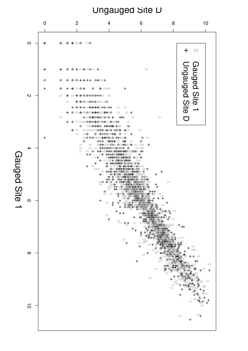
Furthermore, Table 3 shows for all the ungauged sites, the close relatives they have among the Cluster 2 sites that lie within a radius of 100 km, the corresponding global circle distance (GCD) in km, and along with the average of their correlations. This table confirms that indeed does enjoy the highest correlation with its relative. That relationship is further explored in Figure 5 where we see a strong linear relationship between Sites and as our coverage probability assessment had suggested.
In spite of its reliance on the relatives, the DLM does not predict responses at the ungauged sites very accurately as illustrated in Figure 4. That points to problems with this model which will be discussed in the next section.
7 Discussion
In general, the DLM provides a remarkably powerful modelling tool, made practical by advances in statistical computing. However, its substantial computational requirements still limits its applicability. Moreover, the very flexibility that makes it so powerful also imposes an immense burden of choice on the model. This section summarizes critical issues and includes some suggestions for improvement.
Monitoring MCMC convergence
Figure 6 represents the trace plots of model parameters and of two chains from the initial settings in Section 6.1. These two chains seem to mix well after several hundreds iterations, suggesting at first glance the Markov chains have converged.

Autocorrelation and partial
autocorrelation of the simulated Markov chains
However, we know that the autocorrelation, as measured by the autocorrelation function (ACF), is very important when considering the length of the chain. A highly auto–correlated chain needs a long run to yield accurate estimates. Moreover, the partial autocorrelation function (PACF) is also an important index for assessing a Markov chain since large values of the PACF at lag indicates that the next value in the chain is dependent on past values, not just on the most recent ones.

Figure 7 shows the histogram, ACF and PACF plots for the Markov chains used in Section 6.2, after a burn–in period of The ACF plots show the s to be highly autocorrelated, in other words that the –chain does not mix well, potentially leading to biased estimates in Section 6.2. Thinning the chain might reduce that autocorrelation. In other words, using every () generated by the chain could be used to produce the estimates. However, computational challenges make that strategy impractical; we need to use the entire chain.
Relationship between pairs of
and

Our prior assumptions make the model parameters and uncorrelated. Figure 8 shows the relationship between the pairs of these parameters as a way of investigating that assumption. It seems valid except for the – pair in graph That graph shows a weak linear association between and thus pointing to a failure of that assumption for that pair. Since determines spatial variability while determines correlation this relationship seems intriguing. Larger values of tend to go with larger s, i.e., diminished spatial correlation. Why they are coupled in this way is unknown but it should be accounted for in future applications of this model.
Time varying s and s:
empirical coverage probabilities versus nominal credible probabilities
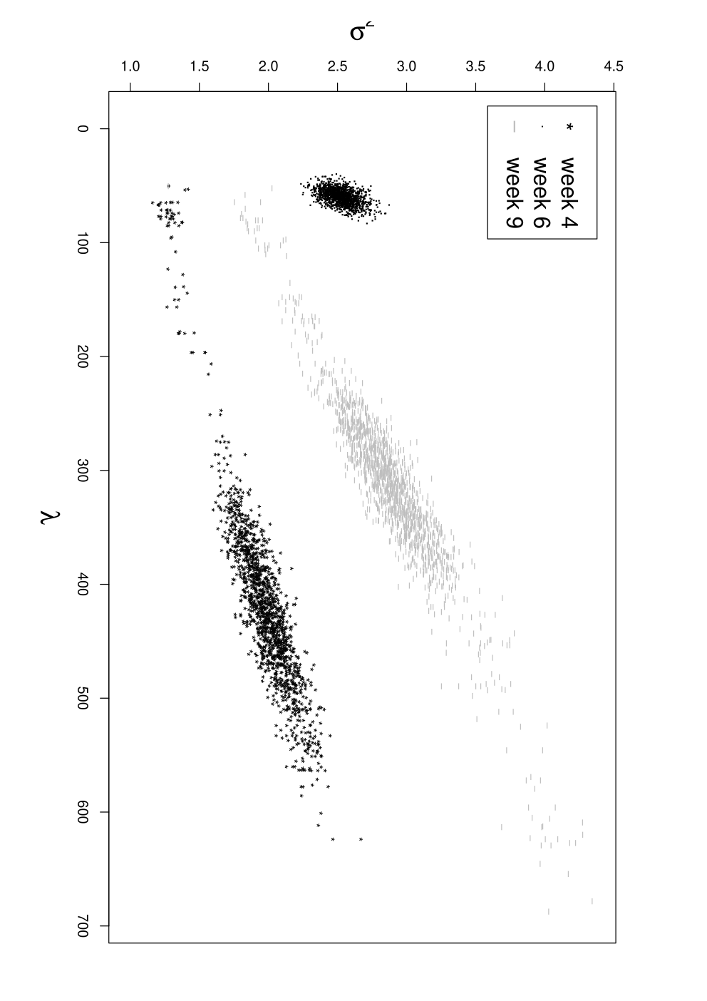
Although we follow Huerta et al. (2004) in assuming the temporal constancy of and it is natural to ask if those generated by the MCMC method change over time. A variant of this issue concerns the time domain of the application. Would the results for these parameters change if we switched from one time span to a longer one containing it? A “yes” to this question would pose a challenge to anyone intending to apply the model, knowing that the choice would have implications for the size of and .
To address these concerns we carried out the following studies:
- (i)
Study Implement the DLM at ungauged sites using weekly data (). Generate Markov chains for and Obtain the coverage probabilities at each ungauged site and week for fixed credibility interval probabilities.
- (ii)
Study Implement the DLM at ungauged sites using week to week data (). Estimate model parameters and interpolate the results at those ungauged sites. Obtain the coverage probabilities at each ungauged site and week for fixed credibility interval probabilities using each week’s data.
- (iii)
Study Fix at week () using values suggested by the Markov chains generated in Study . Then use these as fixed values in the DLM to reduce computation time. In other words, go through all the steps in the algorithm of Section 4.2 but now using only fixed s instead of generating them by a Metropolis–Hasting step. (Note that we are then only using Gibbs sampling and an MCMC blocking scheme.) Compute the corresponding coverage probabilities using at each ungauged site and week for fixed credibility interval probabilities.
Studies and are intended to explore the effect of data and time propagation on the interpolation results. Study aims to pick out any significant difference in the interpolation results when using the fixed rather than using the Markov samples of s. It is also aimed at finding how much time would be saved by avoiding the inefficient Metropolis step. Table 4 shows these fixed s used in Study Table 5 shows the time saved using fixed s against the one using the Metropolis–Hastings algorithm.
Week 54.2 178.5 83.7 405.4 86.6 59.7 199.3 144.1 322.7 Week 142.2 172.7 187.9 315.8 419.0 99.8 260.3 284.8
Time (seconds) Study Data Iteration total Accept(%) Total /Iteration 1,500 0.82 17018 13.8 1,000 0.35 326782 932.3 1,000 1.00 329349 329.3
Figure 9 illustrates the MCMC estimation results obtained in Study It plots the Markov chains of and using weekly data. It is obvious that and vary from week to week, which implies that the constant – model is not tenable over a whole summer for this dataset.

Figure 10 typifies figures in Dou et al. (2007) showing the coverage probabilities for various predictive intervals associated with the interpolators in these three studies. The solid line with bullets represents the results for Study the dotted line with up-triangles for Study and the dashed line with squares for Study These graphs show that the coverage probabilities of Study are similar to that of Study This suggests that we could use the entries in Table 4 as fixed s in the DLM to obtain interpolation results similar to those obtained using the Metropolis–within–Gibbs algorithm.
We have studied the prediction accuracy of the simplest DLM, namely, the first–order polynomial model, in Section 3. As a result, the predictive variances should increase monotonically at successive time points conditional on all the 17 weeks’ data, in the general DLM setting (see Section 3). The plots exhibit a monotonic increasing trend in the coverage probabilities of both Studies and This trend agrees with the graph of the coverage probabilities in Figure 10. Nevertheless, those coverage probabilities of both studies deviate slightly from the expected monotonically increasing trend at some time points because of the time varying effect of – monitored in Figure 9.
On the other hand, Study enjoys significant computational time savings compared with Table 5 suggests that the computation time of the former is almost 2.8 times faster than the latter.
Study shows an intuitively unappealing increase in the uncertainty of interpolation results as time increases; coverage probabilities get larger over time as we see in Table 6. This increase may be interpreted as saying that for the DLM models, the s and s collected from the data should vary over the entire time span of the study, while the prior postulates that they do not vary over that time span. The observed phenomenon may also be due to mis–specification of the model parameter values (See the initial settings for in Section 6.1.).
Ungauged Site A B C Study Week 1 66 65 72 80 78 89 82 80 84 Week 2 73 71 80 76 78 83 79 81 85 Week 3 63 73 82 82 86 91 80 87 93 Week 4 57 74 81 66 83 88 75 87 89 Week 5 53 70 82 68 83 90 59 83 88 Week 6 73 80 88 75 83 89 83 89 93 Week 7 69 88 90 80 92 94 80 93 97 Week 8 66 89 93 66 90 93 71 92 95 Week 9 63 82 88 84 90 94 77 91 96 Week 10 61 87 92 75 93 96 74 94 98 Week 11 58 86 89 77 93 94 68 91 95 Week 12 69 90 92 69 97 96 73 93 98 Week 13 60 87 90 74 91 94 77 94 96 Week 14 67 87 89 81 92 95 69 89 94 Week 15 66 91 95 65 93 96 63 93 97 Week 16 65 91 93 79 94 97 62 91 96 Week 17 68 90 95 81 93 98 71 95 98
Comparing the results of these studies, we find that sometimes, paradoxically, the model gives better results using only one week’s data rather than all. However, Corollary 2 in Section 3 predicts this finding. Because the prior for is the expectation of is implying that and Hence, which is less than (for example, the median of is around 1.21 in Study and even larger in Study ). By the sufficient and necessary condition in Corollary 2, the predictive variance of Study is less than that of Study However, notice that and vary from week to week in which may also lead to the paradox observed in the empirical findings of this section. For example, in (b) of Figure 10, the coverage probability of at the week is larger than that of From the above discussion, we know that the predictive variance of should be less than that of However, of is larger than that of leading an inflated predictive variance of This feature makes it difficult to compare these two predictive variances, but explains the paradox we see in those figures.
8 Summary and Conclusions
To assess the dynamic linear modelling approach to modelling space–time fields, we have applied it to an hourly ozone concentration field over a geographical spatial domain covering most of the eastern United States. To focus that assessment we consider just one cluster of spatial sites we call Cluster 2 during a single ozone season. Moreover, we have used a variant of the dynamic linear modelling approach of Huerta et al. (2004) implemented through MCMC sampling.
Our assessment reveals some difficulties with that very flexible approach and practical challenges that it presents. We also have made some recommendations on improvement.
A curious finding is the posterior dependence of and , in contradiction to our prior assumption. Although the very efficient method Huerta et al. (2004) propose to sampling these parameters is biased, that bias does not appear large enough to account for that phenomenon. We also discovered that the assumption of their constancy over time is untenable.
The coverage probabilities of the model’s posterior predictive credibility intervals over successive weeks, conditional on all weeks of data, increase monotonically. Counter to intuition, that would imply more and more uncertainty as time evolves, an artifact of the modelling that seems hard to explain. A pragmatic way around this undesirable property involves incorporating the length of the time span of the temporal domain into the selection of the values of the model parameters, such as and Section 3 studies the correlation structure of the simplest first–order polynomial DLM and finds reasonable conditions to impose on those parameters.
One further Study tests the proposed constraints on the data. The settings are identical with those in Study except that and are replaced by and respectively, to take account of the longer week time span of our study compared to the one week time span of the application in Huerta et al. (2004). Figure 10 compares Study with the others. Observe that its coverage probabilities behave like those of Study This adjustment does seem to eliminate the undesirable property of increasing credibility bands of Studies and
Another possible approach to dealing with the unsuitability of fixed model parameters uses the composition of Metropolis–Hasting kernels. In other words, we could include these parameters in the Metropolis–Hasting algorithm as in Section 4. We can use six Metropolis–Hasting kernels to sample from the target distribution , updating each component of iteratively, where has defined in Section 2. But, not surprisingly that approach fails because of the extreme computational burden it entails. However, that alternative is the subject of current work along with an approach that admits time varying s and s.
The greatest difficulty involved in the use of the DLM in modelling air pollution space–time fields lies in the computational burden it entails. For that reason, we have not been able to address the geographical domain of real interest, one that embraces sites in the eastern United States, with 120 days of hourly ozone concentrations. In a manuscript under preparation, an alternative hierarchical Bayesian method that can cope with that larger domain will be compared with the DLM where the latter can practically be applied.
Acknowledgements
We thank Prasad Kasibhatla of Nicholas School of the Environment of Duke University for providing the dataset used in this paper and helping with its installation. The funding for the work was provided by the Natural Sciences and Engineering Research Council of Canada.
Appendix A Supplementary results
A.1 Results for Section 3
Only the results about the predictive variances of and are shown in this appendix. The other two cases can be obtained by the same method. Refer to Theorem 1, the predictive variance of can also be written as follows:
The first partial derivatives of this predictive variances regarding to and are given by:
and
respectively. It is straightforward to obtain that is increasing when increases, or decreases, or increases. We next show these properties also hold for By Theorem 1, can also be written as:
The corresponding first partial derivatives are given as follows:
and
respectively, where and
A.2 Results for Section 4.1
The joint posterior distribution for and is given by
Suppose that is, the priors for and are independent of other.
The joint posterior distribution for and can be written as follows:
If the prior for is an inverse gamma distribution with shape parameter and scale parameter then the posterior distribution for is also an inverse gamma distribution with shape parameter and scale parameter
Hence, the posterior density for can be written as follows:
Therefore, the posterior density for is given by
A.3 Results for Section 5
Given the values of the phase parameters, range and variance parameters and the observations until time , the joint distribution of is
where
with a scalar, a by vector, and a by matrix. We use to denote the new distance matrix for the unknown site and the monitoring stations
We then have the conditional posterior distribution of as follows:
| (39) |
Similarly, the conditional posterior distribution for is
| (40) |
Using the observation equation as in Model (1), we have the conditional predictive distribution for as follows:
| (41) |
The software is in http://enviro.stat.ubc.ca.
References
- Burke (2001) Burke, J.M. and Zufall, M.J. and Ozkaynak, H. (2001). A population exposure model for particulate matter: case study results for PM2.5 in Philadelphia, PA, J. Exposure Anal. Environ. Epidemiol.,11, 470–489.
- Calder (2003) Calder, C.A. and Holloman, C.H. and Bortnick, S.M. and Strauss, W.J. and Morara, M. (2003). Relating ambient particulate matter concentration levels to mortality using an exposure simulator, Preprint #725, Dept. Statist., Ohio State U.
- Carter (1994) Carter, C.K. and Kohn, R. (1994). On Gibbs sampling for state space models, Biometrika, 81, 541–553.
- Dou (2007) Dou, Y., Le, N.D. and Zidek, J.V. (2007). A Dynamic Linear Model for Hourly Ozone Concentrations, TR # 228, Dept. Statist., U of British Columbia.
- Gamerman (2006) Gamerman, D. and Lopes H.F. (2006). Markov Chain Monte Carlo: stochastic simulation for Bayesian inference, 2nd Edition, London: Chapman & Hall.
- Huerta (2004) Huerta, G. and Sanso, B. and Stroud, J.R. (2004).A spatio-temporal model for Mexico city ozone levels, JRRSC, 53, 231–248.
- Moller (2003) Moller, J. (2003). Spatial Statistics and Computational Methods, New York: Springer–Verlag.
- Ozone (2005) Ozone (2005). US EPA’s Air Quality Criteria for Ozone and Related Photochemical Oxidants (First External Review Draft), http://cfpub.epa.gov/ ncea/cfm/recordisplay.cfm?deid=149923
- Stroud (2001) Stroud, J.R. and Muller, P. and Sanso, B. (2001). Dynamic models for spatio–temporal data, JRSSB, 63, 673–689.
- West (1997) West, M. and Harrison, J.(1997). Bayesian forcasting and dynamic models, 2nd Edition, New York: Springer.