跳到论文正文
W Papers独立论文阅读器 arXiv:0706.0021 论文正文 计算阅读时间 · 0%
引用这篇论文根据当前论文元数据生成,正式投稿前建议核对。


License: Assumed arXiv.org perpetual non-exclusive license
arXiv:0706.0021v3 [hep-th] 17 Oct 2007

Quantum Fields with Noncommutative Target SpacesPreprint: SU-4252-851

A. P. Balachandran Affiliation: Department of Physics, Syracuse University, Syracuse, NY, 13244-1130, USA.    A. R. Queiroz Affiliation: Centro Internacional de Física da Matéria Condensada, Universidade de Brasília,C.P. 04667, Brasília, DF, Brazil.    A. M. Marques Affiliation: Instituto de Física, Universidade de São Paulo, C.P. 66318, 05315-970,São Paulo, SP, Brazil.E-mail: , , , Email: bal@physics.syr.edu    P. Teotonio-Sobrinho Email: amilcar@fma.if.usp.br Email: amarques@fma.if.usp.br Email: teotonio@fma.if.usp.br Affiliation: Instituto de Física, Universidade de São Paulo, C.P. 66318, 05315-970,São Paulo, SP, Brazil.E-mail: , , , Email: bal@physics.syr.edu
Abstract: 

Quantum field theories (QFT’s) on noncommutative spacetimes are currently under intensive study. Usually such theories have world sheet noncommutativity. In the present work, instead, we study QFT’s with commutative world sheet and noncommutative target space. Such noncommutativity can be interpreted in terms of twisted statistics and is related to earlier work of Oeckl [1], and others [2, 3, 4, 5, 6, 7, 8]. The twisted spectra of their free Hamiltonians has been found earlier by Carmona et al [9, 10]. We review their derivation and then compute the partition function of one such typical theory. It leads to a deformed black body spectrum, which is analysed in detail. The difference between the usual and the deformed black body spectrum appears in the region of high frequencies. Therefore we expect that the deformed black body radiation may potentially be used to compute a GZK cut-off which will depend on the noncommutative parameter θ\theta.

Keywords: 
Noncommutative geometry, Conformal Field Theory, Noncommutative Target Space, GZK Cut-off

1 Introduction

Spacetime noncommutativity is suggested by considerations based on quantum gravity [11] and developments in string theory [12, 13, 14, 15, 16]. Quantum field theories (qft’s) on such spacetimes have been developed first Doplicher et al. [17], and Oeckl [1]. Studies of spacetime symmetries of such models [18, 19] have also led to some insight into their properties, such as Pauli principle violation [2] and the absence of UV-IR mixing [3]. The earlier work of Oeckl [20] using the technology of Hopf algebras have much bearing on such topics and anticipated crucial results. But it is only recently that general attention has focused on the ideas underlying these results.

In order to fully explore the consequences of these results, phenomenological models based on such noncommutative framework are useful. In this regard it would be highly desirable to measure at least a definitive signature of the fact that physics at a scale close to the Planck scale takes place in a noncommutative geometry. One usually expects that signatures of noncommutativity will appear in experiments involving cosmic microwave background (CMB), ultra-high-energy cosmic rays, or other high-energy sources such as those of neutrinos. It is well-known that the CMB radiation shows a black body spectrum with great accuracy, at least for low to medium frequencies. Still we may conjecture that as the measurements become more accurate, deviations from the black body spectrum may be found, particularly in high frequency regions, where data are still not so accurate. Furthermore, the distribution of photons play a key role on the derivation of the GZK cut-off [21]. Upto now estimates of the GZK cut-off are obtained by considering a black body distribution. Deviations from this cut-off may thus provide us signals of noncommutativity.

These facts convince us that any deviation from the usual free massless boson theory may have some influence on the modeling of these experimental facts. One possible source of such deviation is the deformation of the target space of a free massless boson theory. For instance, we may consider a theory with a noncommutative plane as target space. Then a natural question one may raise is how the radiation spectrum is modified by this deformation of the target-space of the free massless boson theory.

We present here a free massless boson theory with commutative base-space and noncommutative target-space. The first results with bearing on such models can be found in the work of Oeckl [1], and can be interpreted in terms of twisted statistics. The idea of deformation of the target space has also been extensively developed in the work11 1 We thank Prof. J. Gamboa and Prof. J. Cortes for calling our attention to their interesting earlier work. of Carmona et al [9, 10]. These works use the earlier work on quantum mechanics with noncommutative target spaces by Nair and Polychronakos [22]. Their physical consequences have also been explored by the same group in [23, 24, 25, 26, 27, 28]. They call the fields with noncommutative target spaces as noncommutative fields. Subsequently Balachandran et al [2, 3, 4, 5, 29] developed and extended the ideas of Oeckl, with emphasis on the link between twisted Poincaré invariance and twisted statistics. Note that it can be argued that spacetime and target space noncommutativity are linked to each other by symmetry principles.

Our treatment of deformed conformal symmetry in section 2.3 is new. Also unlike Carmona et al, we consider nonconstant deformation parameters and discuss the deformed black body radiation spectrum in detail. This study can acquire significance from the point of view of of phenomenology.

Sections 2 and 3 contain many results already obtained by [9, 10], although perhaps our derivation of their results is slighty different. They are included here for completeness.

The present work is organised as follows. In section 2, we construct a free massless boson theory with noncommutative ℝ2\mathbb{R}^{2}, hereafter referred to as the deformed theory, for the case where the base space is a (1+1)(1+1)-d space given by the cylinder S1×ℝS^{1}\times\mathbb{R}. After constructing the Hamiltonian formulation of this theory and quantizing it, we calculate 22-point correlation functions and also see how the conformal generators are modified by the introduction of noncommutativity. The results obtained in this section are, then, generalised to a more realistic scenario in section 3. In this section, we show the same theory, but now with the (3+1)(3+1)-d base space given by S1×S1×S1×ℝS^{1}\times S^{1}\times S^{1}\times\mathbb{R}. Then, using this (3+1)(3+1)-d theory, we study the radiation law for the deformed theory and compare it with the usual commutative theory, i.e., the black body radiation. Concluding remarks are section 5.

2 Deformed (1+1)(1+1)-d Theory

In this section we construct a deformed version of a (1+1)(1+1)-d theory. For that we start with a target space ℝ2\mathbb{R}^{2} as a group manifold. Then we use a twisting procedure on the group ℝ2\mathbb{R}^{2}, so that it becomes the noncommutative plane.

The phase space T∗​ℝ2T^{*}\mathbb{R}^{2} of a single particle in ℝ2\mathbb{R}^{2} has a natural group structure. It is the semi-direct product of ℝ2\mathbb{R}^{2} with ℝ2\mathbb{R}^{2}. The generators of its Lie algebra can be taken to be coordinates xa,a=1,2x^{a},a=1,2, and momenta pap_{a}. The algebra generated by xax^{a} and pap_{a} are given by

[xa,xb]\displaystyle\left[x^{a},x^{b}\right] =\displaystyle= 0\displaystyle 0 (1)
[pa,pb]\displaystyle\left[p_{a},p_{b}\right] =\displaystyle= 0\displaystyle 0 (2)
[xa,pb]\displaystyle\left[x^{a},p_{b}\right] =\displaystyle= i​δba.\displaystyle i\delta^{a}_{b}\,. (3)

Functions on ℝ2\mathbb{R}^{2} are thus commutative and pap_{a} acts as derivative on these functions.

We now twist (or deform) the generators of the above algebra into x^a,p^b\hat{x}^{a},{\hat{p}}_{b} and thus obtain a new algebra. The algebra of derivatives are not deformed, but the function algebra is. The twisted algebra reads [30, 22]

[x^a,x^b]\displaystyle\left[\widehat{x}^{a},\widehat{x}^{b}\right] =\displaystyle= i​ϵa​b​θ≡i​θa​b\displaystyle i\epsilon^{ab}\theta\equiv i\theta^{ab} (4)
[p^a,p^b]\displaystyle\left[\widehat{p}_{a},\widehat{p}_{b}\right] =\displaystyle= 0\displaystyle 0 (5)
[x^a,p^b]\displaystyle\left[\widehat{x}^{a},\widehat{p}_{b}\right] =\displaystyle= i​δba.\displaystyle i\delta^{a}_{b}. (6)

The so-called non-commutativity parameter θa​b=−θb​a\theta^{ab}=-\theta^{ba} is as usual taken as a constant for the present.

We can relate the hatted generators (noncommutative ones) to the usual generators by the deformation map22 2 The analogue of the map xa→x^ax^{a}\to\hat{x}^{a} first appeared in the works of Grosse [31], Zamolodchikov and Zamolodchikov [32] and Faddeev [33]. It is sometimes called a dressing transformation.

x^a\displaystyle\widehat{x}^{a} =\displaystyle= xa−12​θa​b​pb,\displaystyle x^{a}-\frac{1}{2}\theta^{ab}p_{b},
p^a\displaystyle\widehat{p}^{a} =\displaystyle= pa.\displaystyle p^{a}. (7)

In what follows, we will generalize the above deformation map to the case of a scalar field theory.

We start with a free real massless bosonic field. Its base space is a cylinder with circumference RR and its target space is ℝ2\mathbb{R}^{2}, i.e.,

φ:S1×ℝ⟶ℝ2(x,t)⟼φ⁡(x,t)\begin{array}[]{cccl}\varphi:&S^{1}\times\mathbb{R}&\longrightarrow&\mathbb{R}^{2}\\ &(x,t)&\longmapsto&\varphi(x,t)\end{array}

The field components will be denoted φi\varphi^{i} where i=1,2i=1,2. The compactification of the space coordinate makes each field component periodic in the variable xx, i.e.,

φi​(x+R,t)≡φi​(x,t).\varphi^{i}(x+R,t)\equiv\varphi^{i}(x,t)\,.

The field components φi​(x,t)\varphi^{i}(x,t) may be written as a Fourier expansion

φi​(x,t)=∑ne2​π​iR​n​x​φni​(t),\varphi^{i}(x,t)=\sum_{n}\;e^{\frac{2\pi i}{R}nx}\;\varphi^{i}_{n}(t)\;, (8)

where the Fourier components are

φni​(t)=1R​∫d​x​e−2​π​iR​n​x​φi​(x,t)=φ−ni​(t)∗.\varphi^{i}_{n}(t)=\frac{1}{R}\int dx\;e^{-\frac{2\pi i}{R}nx}\;\varphi^{i}(x,t)\;=\varphi_{-n}^{i}(t)^{*}. (9)

The Lagrangian for the free field is

L=g2​∫d​x​[(∂tφi)2−(∂xφi)2]L=\frac{g}{2}\int dx\big[\big(\partial_{t}\varphi^{i}\big)^{2}-\big(\partial_{x}\varphi^{i}\big)^{2}\big] (10)

where there is an implicit sum over the target space coordinate index ii.

In terms of Fourier modes, the above Lagrangian is

L=g​R2​∑i,n{φ˙ni​φ˙−ni−(2​π​nR)2​φni​φ−ni}.L=\frac{gR}{2}\sum_{i,n}\bigg\{\dot{\varphi}^{i}_{n}\dot{\varphi}^{i}_{-n}-\bigg(\frac{2\pi n}{R}\bigg)^{2}\varphi^{i}_{n}\varphi^{i}_{-n}\bigg\}\;. (11)

It is a standard exercise to check that the theory defined by the Lagrangian (10) possesses conformal invariance. This is verified by showing that the energy-momentum tensor is traceless.

We can define the momenta conjugate to φin=φ−ni∗\varphi^{i}_{n}=\varphi_{-n}^{i~*} as

πin=∂L∂φ˙ni=gRφ˙i−n=π−ni∗.\pi^{i}_{n}=\frac{\partial L}{\partial\dot{\varphi}^{i}_{n}}=gR\,\dot{\varphi}^{i}_{-n}=\pi_{-n}^{i~*}. (12)

We then have the following commutation relations:

[φmi,φnj]=[πmi,πnj]=0[φmi,πnj]=i​δm​n​δi​j.\left[\varphi_{m}^{i},\varphi_{n}^{j}\right]=\left[\pi_{m}^{i},\pi_{n}^{j}\right]=0\hskip 28.45274pt\left[\varphi_{m}^{i},\pi_{n}^{j}\right]=i\delta_{mn}\delta^{ij}\;. (13)

The Hamiltonian for (11) is

H=∑i(π0i)22​g​R+12​g​R​∑i,n≠0{πni​π−ni+(2​π​|n|​g)2​φni​φ−ni}.H=\sum_{i}\frac{(\pi_{0}^{i})^{2}}{2gR}+\frac{1}{2gR}\sum_{i,n\neq 0}\big\{\pi^{i}_{n}\pi^{i}_{-n}+(2\pi|n|g)^{2}\varphi^{i}_{n}\varphi^{i}_{-n}\big\}\;. (14)

For n≠0n\neq 0, it is equivalent to an infinite set of decoupled harmonic oscillators with frequencies

ωn=2​π​|n|R.\omega_{n}=\frac{2\pi|n|}{R}\;. (15)

The first term in the l.h.s. of equation (14) is known as the zero mode. We will mostly ignore it in the rest of these notes. It will not affect our conclusions. The hermiticity of φi\varphi^{i} implies that

φni†(t)=1R∫dxe2​π​i​n​xRφi(x,t)=φ−ni(t)\varphi_{n}^{i\;\dagger}(t)=\frac{1}{R}\int dxe^{\frac{2\pi inx}{R}}\varphi^{i}(x,t)=\varphi^{i}_{-n}(t) (16)

and

πni†=πi−n.\pi_{n}^{i\;\dagger}=\pi^{i}_{-n}\;. (17)

We now generalize the deformation map (2) to the above scalar field theory. We take ordinary field theory with target ℝ2\mathbb{R}^{2} described by canonical pairs φa,πa\varphi^{a},\pi_{a}, a=1,2a=1,2, and then use the map (2) so that

φ^a​(x,t)\displaystyle\hat{\varphi}^{a}(x,t) =\displaystyle= φa​(x,t)−12​θa​b​πb​(x,t),\displaystyle\varphi^{a}(x,t)-\frac{1}{2}\theta^{ab}\pi_{b}(x,t), (18)
π^a​(x,t)\displaystyle\hat{\pi}_{a}(x,t) =\displaystyle= πa​(x,t).\displaystyle\pi_{a}(x,t)\;. (19)

In the case where θa​b=θ​ϵa​b\theta^{ab}=\theta\epsilon^{ab}, with θ\theta chosen as a constant, the corresponding equal time commutation relations are

[φ^a​(x,t),φ^b​(y,t)]\displaystyle\left[\hat{\varphi}^{a}(x,t),\hat{\varphi}^{b}(y,t)\right] =\displaystyle= i​ϵa​b​θ​δ​(x−y),\displaystyle i\epsilon^{ab}\theta\delta(x-y), (20)
[π^a​(x,t),π^b​(y,t)]\displaystyle\left[\hat{\pi}_{a}(x,t),\hat{\pi}_{b}(y,t)\right] =\displaystyle= 0,\displaystyle 0, (21)
[φ^a​(x,t),π^b​(y,t)]\displaystyle\left[\hat{\varphi}^{a}(x,t),\hat{\pi}_{b}(y,t)\right] =\displaystyle= i​δba​δ​(x−y).\displaystyle i\,\delta^{a}_{b}\delta(x-y). (22)

These are the relations of [9, 10] in the limit of their BB becoming zero.

In what follows, we are going to redefine θ​δ​(x−y)\theta\delta(x-y) such that

θ⁡(σ)=θ2​π​σ​e−(x−y)22​σ2\theta(\sigma)=\frac{\theta}{\sqrt{2\pi}\sigma}e^{-\frac{(x-y)^{2}}{2\sigma^{2}}} (23)

which is the previous constant θ\theta times a function of a new parameter σ\sigma. This new parameter σ\sigma introduces a new distance scale in the equal time commutation relations for the fields:

[φ^a​(x,t),φ^b​(y,t)]=i​ϵa​b​θ2​π​σ​e−(x−y)22​σ2.\left[\hat{\varphi}^{a}(x,t),\hat{\varphi}^{b}(y,t)\right]=\frac{i\epsilon^{ab}\theta}{\sqrt{2\pi}\sigma}e^{-\frac{(x-y)^{2}}{2\sigma^{2}}}\;.\\ (24)

It is important to note that these new commutation relations reduces to those in (20) in the limit σ→0\sigma\rightarrow 0. We note further the fact that while the new θ⁡(σ)\theta(\sigma) is dimensionless, because θ⁡(σ)\theta(\sigma) substitutes the previous θ​δ​(x−y)\theta\delta(x-y), the θ\theta in θ⁡(σ)\theta(\sigma) still has the dimension of (length)−2(\textrm{length})^{-2}.

In more than two dimensions, it is not easy to introduce spacetime dependence in the noncommutative parameter (called also θμ​ν\theta^{\mu\nu}) of the Moyal plane [34], because of constraints from Jacobi identity. But here we twist the target of fields, so that this problem does not arise.

The above deformed algebra describes a field with noncommutative plane as target. The degree of non-commutativity is regulated by a new parameter σ\sigma.

We can describe the deformed algebra in terms of the Fourier modes

φ^a=∑ne2​π​iR​n​x​φ^na.\hat{\varphi}^{a}=\sum_{n}e^{\frac{2\pi i}{R}nx}\hat{\varphi}_{n}^{a}. (25)

Then the “dressing transformation”

φ^na\displaystyle\hat{\varphi}_{n}^{a} =\displaystyle= φna−12​R​ϵa​b​θ​(n)​π−nb,\displaystyle\varphi_{n}^{a}-\frac{1}{2R}\epsilon^{ab}\theta(n)\pi_{-n}^{b}, (26)
π^na\displaystyle\hat{\pi}_{n}^{a} =\displaystyle= πna,\displaystyle\pi_{n}^{a}, (27)

where RR is the circumference of the base space cylinder S1×ℝS^{1}\times\mathbb{R} and

θ⁡(n)=θ​e−2​π2​σ2​n2R2.\theta(n)=\theta\;e^{-\frac{2\pi^{2}\sigma^{2}n^{2}}{R^{2}}}\,. (28)

reproduces the Fourier components of (24), (21) and (22):

[φ^na,φ^mb]\displaystyle\left[\hat{\varphi}_{n}^{a},\hat{\varphi}_{m}^{b}\right] =\displaystyle= iR​ϵa​b​θ​(n)​δn+m,0,\displaystyle\frac{i}{R}\epsilon^{ab}\theta(n)\delta_{n+m,0}, (29)
[π^na,π^mb]\displaystyle\left[\hat{\pi}_{n}^{a},\hat{\pi}_{m}^{b}\right] =\displaystyle= 0,\displaystyle 0, (30)
[φ^na,π^mb]\displaystyle\left[\hat{\varphi}_{n}^{a},\hat{\pi}_{m}^{b}\right] =\displaystyle= i​δa​b​δm​n.\displaystyle i\,\delta^{ab}\delta_{mn}. (31)

(Notice that [θ⁡(n)]=dimension of ​θ​(n)=length[\theta(n)]=\textrm{dimension of }\theta(n)=\textrm{length}.)

We can write the Hamiltonian in terms of the deformed fields and momenta, using equations (18), (26) and (27). Then, the Hamiltonian, without the zero mode term, reads

H\displaystyle H =\displaystyle= 12​g​R​∑i,n{π^ni​π^−ni+(2​π​|n|​g)2​φ^ni​φ^−ni}\displaystyle\frac{1}{2gR}\sum_{i,n}\left\{\hat{\pi}_{n}^{i}\,\hat{\pi}_{-n}^{i}+(2\pi|n|g)^{2}\,\hat{\varphi}^{i}_{n}\,\hat{\varphi}^{i}_{-n}\right\} (32)
=\displaystyle= 12​g​R∑i,j,n{[1+(π​g​|n|​θ​(n)R)2]πniπ−ni+\displaystyle\frac{1}{2gR}\sum_{i,j,n}\left\{\left[1+\left(\frac{\pi g|n|\theta(n)}{R}\right)^{2}\right]\,\pi_{n}^{i}\,\pi_{-n}^{i}\right.+
+(2π|n|g)2φniφ−ni−(2​π​|n|​g)2Rϵi​jθ(n)φniπnj}.\displaystyle\left.\phantom{\frac{1}{2gR}\sum_{(i,k,n)}\;}+(2\pi|n|g)^{2}\,\varphi_{n}^{i}\,\varphi_{-n}^{i}-\frac{(2\pi|n|g)^{2}}{R}\epsilon_{ij}\theta(n)\varphi_{n}^{i}\pi_{n}^{j}\right\}\;.

2.1 The Schwinger Representation and the Construction of the Fock Space

We can construct a Fock space, since the Hamiltonian (32) can be diagonalised using the Schwinger representation of S​U​(2)SU(2). It is remarkable that the last term of the Hamiltonian in equation (32) is proportional to the zz-component of the angular momentum LzL_{z}. This fact motivates the use of the Schwinger representation.

First, let us rewrite the full Hamiltonian (32) as

H=∑i(π0i)22​g​R+∑i,j,n≠0(Ωn22​g​R​πni​π−ni+g​R2​ωn2​φni​φ−ni−g2​θ​(n)​ωn2​ϵi​j​φni​πnj),H=\sum_{i}\frac{(\pi_{0}^{i})^{2}}{2gR}+\sum_{i,j,n\neq 0}\left(\;\frac{\Omega^{2}_{n}}{2gR}\;\pi_{n}^{i}\,\pi_{-n}^{i}\,+\frac{gR}{2}\;\omega_{n}^{2}\,\varphi_{n}^{i}\,\varphi_{-n}^{i}-\frac{g}{2}\theta(n)\,\omega_{n}^{2}\,\epsilon_{ij}\varphi_{n}^{i}\pi_{n}^{j}\;\right), (33)

where

Ωn2=1+(π​g​|n|​θ​(n)R)2andωn=2​π​|n|R.\Omega^{2}_{n}=1+\left(\frac{\pi g|n|\theta(n)}{R}\right)^{2}\hskip 28.45274pt\mathrm{and}\hskip 28.45274pt\omega_{n}=\frac{2\pi|n|}{R}\;. (34)

It is important to note that in the limit θ→0\theta\rightarrow 0, we have θ⁡(n)→0\theta(n)\rightarrow 0 and Ωn2→1\Omega^{2}_{n}\rightarrow 1. This limit takes the Hamiltonian (33) to the usual Hamiltonian for the free massless bosons upon a commutative target space.

Separating the zero mode contribution H0H_{0}, we have

H=H0+∑i,j,n≠0(Ωn22​g​R​πni​π−ni+g​R2​ωn2​φni​φ−ni−g2​θ​(n)​ω2​ϵi​k​φni​πnk).H=H_{0}+\sum_{i,j,n\neq 0}\left(\frac{\Omega^{2}_{n}}{2gR}\,\pi_{n}^{i}\,\pi_{-n}^{i}+\frac{gR}{2}\;\omega_{n}^{2}\,\varphi_{n}^{i}\,\varphi_{-n}^{i}-\frac{g}{2}\theta(n)\,\omega^{2}\,\epsilon_{ik}\,\varphi_{n}^{i}\pi_{n}^{k}\right). (35)

Therefore, the Hamiltonian may be written as

H=H0+∑n≠0(Hn−g2​θ​(n)​ωn2​Jnz),H=H_{0}+\sum_{n\neq 0}\;\big({H}_{n}-\frac{g}{2}\,\theta(n)\omega_{n}^{2}\,J_{n}^{z}\;\big), (36)

where

H0=∑iπ0i22​g​R,{H_{0}}=\sum_{i}\frac{{\pi_{0}^{i}}^{2}}{2gR}\;, (37)
Hn=∑i(Ωn22​g​R​πni​π−ni+g​R2​ωn2​φni​φ−ni)H_{n}=\sum_{i}\left(\frac{\Omega^{2}_{n}}{2gR}\,\pi_{n}^{i}\,\pi_{-n}^{i}+\frac{gR}{2}\,\omega_{n}^{2}\,\varphi_{n}^{i}\,\varphi_{-n}^{i}\right) (38)

and

Jnz=∑i,jϵi​j​φni​πnj.J_{n}^{z}=\sum_{i,j}\epsilon_{ij}\,\varphi_{n}^{i}\,\pi_{n}^{j}\;. (39)

Hn{H}_{n} alone is the Hamiltonian of a harmonic oscillator with frequency Ωn​ωn\Omega_{n}\omega_{n}, which can be easily diagonalised if we note that it can be rewritten as

Hn=∑i(12​M​πni​π−ni+12​M​ω¯n2​φni​φ−ni).H_{n}=\sum_{i}\left(\frac{1}{2M}\,\pi_{n}^{i}\,\pi_{-n}^{i}+\frac{1}{2}\,M\bar{\omega}_{n}^{2}\,\varphi_{n}^{i}\,\varphi_{-n}^{i}\right). (40)

This is the traditional form of the harmonic oscillator Hamiltonian, where

M=g​RΩn2andω¯n=Ωn​ωn.M=\frac{gR}{\Omega^{2}_{n}}\hskip 28.45274pt\mathrm{and}\hskip 28.45274pt\bar{\omega}_{n}=\Omega_{n}\,\omega_{n}. (41)

We may now define annihilation and creation operators. For n≠0n\neq 0:

ani=Δn2​(φni+i​π−niΔn)ani†=Δn2​(φ−ni−i​πniΔn)a_{n}^{i}=\sqrt{\frac{\Delta_{n}}{2}}\bigg(\varphi_{n}^{i}+i\frac{\pi_{-n}^{i}}{\Delta_{n}}\bigg)\hskip 28.45274pt{a_{n}^{i}}^{\dagger}=\sqrt{\frac{\Delta_{n}}{2}}\bigg(\varphi_{-n}^{i}-i\frac{\pi_{n}^{i}}{\Delta_{n}}\bigg) (42)

where

Δn=M​ω¯n=g​R​ωnΩn=2​π|n|gΩn,\Delta_{n}=M\bar{\omega}_{n}=\frac{gR\omega_{n}}{\Omega_{n}}=\frac{2\pi\,|n|\,g}{\Omega_{n}}\;, (43)

and, as usual,

[ami,anj]=[ami†,anj†]=0[ami,anj†]=δm​n​δi​j\left[a^{i}_{m},a^{j}_{n}\right]=\left[{a^{i}_{m}}^{\dagger},{a^{j}_{n}}^{\dagger}\right]=0\hskip 28.45274pt\left[a^{i}_{m},{a^{j}_{n}}^{\dagger}\right]=\delta_{mn}\delta^{ij}\; (44)

It is now easy to check that

φni=12​Δn​(ani+a−ni†)πni=−i​Δn2​(a−ni−ani†)\varphi_{n}^{i}=\frac{1}{\sqrt{2\Delta_{n}}}(a_{n}^{i}+{a_{-n}^{i}}^{\dagger})\hskip 28.45274pt\pi_{n}^{i}=-i\sqrt{\frac{\Delta_{n}}{2}}({a}_{-n}^{i}-{a_{n}^{i}}^{\dagger}) (45)

and that if we make θ→0\theta\rightarrow 0, we have Ωn→1\Omega_{n}\rightarrow 1 and Δn→2​π​|n|​g\Delta_{n}\rightarrow 2\pi|n|g and in this limit ania_{n}^{i} and ani†{a_{n}^{i}}^{\dagger} reduce to their usual (commutative space-time) version.

Now, in terms of these annihilation and creation operators the Hamiltonian becomes

Hn=∑iωn​Ωn2​(ani​ani†+a−ni†​a−ni){H}_{n}=\sum_{i}\frac{\omega_{n}\,\Omega_{n}}{2}\;({a_{n}^{i}}\,{a_{n}^{i}}^{\dagger}+{a_{-n}^{i}}^{\dagger}\,{a_{-n}^{i}}) (46)

which, using some algebra, can be written as (the :⁣::\ : symbols stand for the usual normal ordering of operators)

∑n≠0Hn\displaystyle\sum_{n\neq 0}H_{n} =\displaystyle= ∑i,n≠0ωn​Ωn2:(ani​ani†+a−ni†​a−ni):\displaystyle\sum_{i,n\neq 0}\frac{\omega_{n}\,\Omega_{n}}{2}:({a_{n}^{i}}\,{a_{n}^{i}}^{\dagger}+{a_{-n}^{i}}^{\dagger}\,{a_{-n}^{i}}): (47)
=\displaystyle= ∑i,n≠0ωn​Ωn2​(ani†​ani+a−ni†​a−ni)\displaystyle\sum_{i,n\neq 0}\frac{\omega_{n}\,\Omega_{n}}{2}\;({a_{n}^{i}}^{\dagger}\,{a_{n}^{i}}+{a_{-n}^{i}}^{\dagger}\,{a_{-n}^{i}})
=\displaystyle= ∑i,n≠0ωn​Ωn​ani†​ani.\displaystyle\sum_{i,n\neq 0}\omega_{n}\,\Omega_{n}\;{a_{n}^{i}}^{\dagger}\,{a_{n}^{i}}.

Accordingly, for the angular momentum term we get

∑n≠0Jnz=−∑n≠0iϵi​jani†anj,\sum_{n\neq 0}J_{n}^{z}=-\sum_{n\neq 0}i\;\epsilon_{ij}\;{a_{n}^{i}}^{\dagger}{a_{n}^{j}}\,, (48)

so that we can finally write the complete Hamiltonian as

H=∑i(π0i)22​g​R+∑n≠0ωn​Ωn​ani†​ani−i​g2​θ​(n)​ωn2​ϵi​j​ani†​anj.H=\sum_{i}\frac{(\pi^{i}_{0})^{2}}{2gR}+\sum_{n\neq 0}\omega_{n}\,\Omega_{n}\;{a_{n}^{i}}^{\dagger}a_{n}^{i}-i\frac{g}{2}\,\theta(n)\,\omega_{n}^{2}\epsilon_{ij}\,{a_{n}^{i}}^{\dagger}{a_{n}^{j}}\,. (49)

The appearance of the angular momentum term may be seen as a signature of the well-known relation between noncommutative plane and a plane embedded in a magnetic field perpendicular to it.

Now we define new annihilation and creation operators

An1=12​(an1−i​an2)An2=12​(an1+i​an2)A^{1}_{n}=\frac{1}{\sqrt{2}}(a_{n}^{1}-ia^{2}_{n})\hskip 56.9055ptA^{2}_{n}=\frac{1}{\sqrt{2}}(a_{n}^{1}+ia^{2}_{n}) (50)

such that

[Ani,Amj†]=δn​m​δi​j.\left[A^{i}_{n},{A^{j}_{m}}^{\dagger}\right]=\delta_{nm}\delta^{ij}\;.

Using equations (45) and (50), we can check that the field components can be written as

φn1\displaystyle\varphi_{n}^{1} =\displaystyle= 12​Δn(An1+A−n1†+An2+A−n2†)\displaystyle\frac{1}{2\sqrt{\Delta_{n}}}(A_{n}^{1}+A_{-n}^{1\dagger}+A_{n}^{2}+A_{-n}^{2\dagger}) (51)
φn2\displaystyle\varphi_{n}^{2} =\displaystyle= i2​Δn(An1−A−n1†−An2+A−n2†).\displaystyle\frac{i}{2\sqrt{\Delta_{n}}}(A_{n}^{1}-A_{-n}^{1\dagger}-A_{n}^{2}+A_{-n}^{2\dagger})\;. (52)

In terms of these AA’s and A†A^{\dagger}’s the Hamiltonian reads

H\displaystyle H =\displaystyle= H0+∑n≠0ωn​{(Ωn+π|n|g​θ​(n)R)​An1†​An1+(Ωn−π|n|g​θ​(n)R)​An2†​An2}\displaystyle H_{0}+\sum_{n\neq 0}\omega_{n}\bigg\{\left(\Omega_{n}+\frac{\pi|n|g\theta(n)}{R}\right){A_{n}^{1}}^{\dagger}A_{n}^{1}+\left(\Omega_{n}-\frac{\pi|n|g\theta(n)}{R}\right){A_{n}^{2}}^{\dagger}A_{n}^{2}\bigg\} (53)
=\displaystyle= ∑n≠0ωn​{Λn1​An1†​An1+Λn2​An2†​An2}\displaystyle\sum_{n\neq 0}\omega_{n}\bigg\{\Lambda^{1}_{n}\,{A_{n}^{1}}^{\dagger}A_{n}^{1}+\Lambda^{2}_{n}\,{A_{n}^{2}}^{\dagger}A_{n}^{2}\bigg\}

where

Λn1\displaystyle\Lambda_{n}^{1} =\displaystyle= Ωn+π|n|g​θ​(n)R,\displaystyle\Omega_{n}+\frac{\pi|n|g\theta(n)}{R}, (54)
Λn2\displaystyle\Lambda_{n}^{2} =\displaystyle= Ωn−π|n|g​θ​(n)R.\displaystyle\Omega_{n}-\frac{\pi|n|g\theta(n)}{R}\;. (55)

Notice that an important effect of introducing noncommutativity is the splitting of the energy levels of each individual mode that constitutes the whole system. One should recall the resemblance of this effect to the well-known Zeeman effect in a quantum system in the presence of a magnetic field.

Time evolution of the AnA_{n}’s and An†A_{n}^{\dagger}’s is given by

An1​(t)=An1​(0)​e−i​ωn​Λn1​t,An2​(t)=An2​(0)​e−i​ωn​Λn2​t,A_{n}^{1}(t)=A^{1}_{n}(0)\,e^{-i\omega_{n}\Lambda^{1}_{n}\,t}\;,\hskip 42.67912ptA_{n}^{2}(t)=A^{2}_{n}(0)\,e^{-i\omega_{n}\Lambda^{2}_{n}\,t}\;, (56)
Am1†​(t)=Am1†​(0)​ei​ωm​Λm1​t,Am2†​(t)=Am2†​(0)​ei​ωm​Λm2​t.{A_{m}^{1}}^{\dagger}(t)={A^{1}_{m}}^{\dagger}(0)\,e^{i\omega_{m}\Lambda^{1}_{m}\,t}\;,\hskip 42.67912pt{A_{m}^{2}}^{\dagger}(t)={A^{2}_{m}}^{\dagger}(0)\,e^{i\omega_{m}\Lambda^{2}_{m}\,t}\;. (57)

which together with equation (51) and (52) gives, (omitting zero modes),

φ1​(x,t)\displaystyle\varphi^{1}(x,t) =\displaystyle= 18​π​g∑n≠0Ωn|n|{An1e2​π​iR​(n​x−|n|​Λn1​t)+An1†e−2​π​iR​(n​x−|n|​Λn1​t)+\displaystyle\frac{1}{\sqrt{8\pi g}}\sum_{n\neq 0}\sqrt{\frac{\Omega_{n}}{|n|}}\bigg\{A^{1}_{n}\,e^{\frac{2\pi i}{R}(nx-|n|\Lambda^{1}_{n}t)}+A^{1\dagger}_{n}\,e^{-\frac{2\pi i}{R}(nx-|n|\Lambda^{1}_{n}t)}+ (58)
+An2e2​π​iR​(n​x−|n|​Λn2​t)+An2†e−2​π​iR​(n​x−|n|​Λn2​t)}\displaystyle\phantom{\frac{1}{\sqrt{8\pi g}}\sum_{n\neq 0}\bigg\{}+A^{2}_{n}\,e^{\frac{2\pi i}{R}(nx-|n|\Lambda^{2}_{n}t)}+A^{2\dagger}_{n}\,e^{-\frac{2\pi i}{R}(nx-|n|\Lambda^{2}_{n}t)}\bigg\}

and

φ2​(x,t)\displaystyle\varphi^{2}(x,t) =\displaystyle= i8​π​g∑n≠0Ωn|n|{An1e2​π​iR​(n​x−|n|​Λn1​t)−An1†e−2​π​iR​(n​x−|n|​Λn1​t)−\displaystyle\frac{i}{\sqrt{8\pi g}}\sum_{n\neq 0}\sqrt{\frac{\Omega_{n}}{|n|}}\bigg\{A^{1}_{n}\,e^{\frac{2\pi i}{R}(nx-|n|\Lambda^{1}_{n}t)}-A^{1\dagger}_{n}\,e^{-\frac{2\pi i}{R}(nx-|n|\Lambda^{1}_{n}t)}- (59)
−An2e2​π​iR​(n​x−|n|​Λn2​t)+An2†e−2​π​iR​(n​x−|n|​Λn2​t)}\displaystyle\phantom{\frac{1}{\sqrt{8\pi g}}\sum_{n\neq 0}\bigg\{}-A^{2}_{n}\,e^{\frac{2\pi i}{R}(nx-|n|\Lambda^{2}_{n}t)}+A^{2\dagger}_{n}\,e^{-\frac{2\pi i}{R}(nx-|n|\Lambda^{2}_{n}t)}\bigg\}

2.2 Correlation Functions

Given the new fields (58) and (59) we can evaluate the two-point correlation functions, e.g., for φ1\varphi^{1}:

⟨φ1​(x1,t1)​φ1​(x2,t2)⟩\displaystyle\mathinner{\langle{\varphi^{1}(x_{1},t_{1})\varphi^{1}(x_{2},t_{2})}\rangle} =\displaystyle= 18​π​g∑n≠0Ωnne2​π​i​n​xR​(x1−x2)×\displaystyle\frac{1}{8\pi g}\sum_{n\neq 0}\frac{\Omega_{n}}{n}\;e^{\frac{2\pi inx}{R}(x_{1}-x_{2})}\times (60)
×[e−2​π​iR​|n|​Λn1​(t1−t2)+e−2​π​iR​|n|​Λn2​(t1−t2)].\displaystyle\phantom{\frac{1}{8\pi g}}\times\left[e^{-\frac{2\pi i}{R}|n|\Lambda^{1}_{n}(t_{1}-t_{2})}+e^{-\frac{2\pi i}{R}|n|\Lambda^{2}_{n}(t_{1}-t_{2})}\right].

Taking the limit θ→0\theta\rightarrow 0 of this expression we get

⟨φ1​(x1,t1)​φ1​(x2,t2)⟩=14​π​g​∑n≠01n​e2​π​i​n​xR​(x1−x2)​e−i​ωn​(t1−t2),\mathinner{\langle{\varphi^{1}(x_{1},t_{1})\varphi^{1}(x_{2},t_{2})}\rangle}=\frac{1}{4\pi g}\sum_{n\neq 0}\frac{1}{n}\;e^{\frac{2\pi inx}{R}(x_{1}-x_{2})}\;e^{-i\omega_{n}(t_{1}-t_{2})}\;, (61)

which is exactly what we would get for the two-point correlation function on the commutative plane.

The same calculation can be performed for φ2​(x,t)\varphi^{2}(x,t) with a similar result. Furthermore:

⟨φ1​(x1,t1)​φ2​(x2,t2)⟩=0.\mathinner{\langle{\varphi^{1}(x_{1},t_{1})\varphi^{2}(x_{2},t_{2})}\rangle}=0\;. (62)

2.3 The Deformed Conformal Generators

We study in the sequel how the conformal generators are deformed by the deformations introduced by the noncommutativity of the target space.

The deformed Hamiltonian is written in terms of the hatted operators as

H=12​g​R​∑i(π0i)2+12​g​R​∑i,n(π^ni​π^−ni+(2​π​|n|​g)2​φ^ni​φ^−ni).H=\frac{1}{2gR}\sum_{i}(\pi_{0}^{i})^{2}+\frac{1}{2gR}\sum_{i,n}\left(\hat{\pi}_{n}^{i}\,\hat{\pi}_{-n}^{i}+(2\pi|n|g)^{2}\,\hat{\varphi}^{i}_{n}\,\hat{\varphi}^{i}_{-n}\right). (63)

It can be diagonalised if we define the deformed creation and annihilation operators as

a^ni\displaystyle{\hat{a}^{i}_{n}} =\displaystyle= 14​π|n|g​(2​π​g​|n|​φ^ni+i​π^−ni),\displaystyle\frac{1}{\sqrt{4\pi|n|g}}\big(2\pi g|n|\hat{\varphi}^{i}_{n}+i\hat{\pi}_{-n}^{i}\big), (64)
a^i†n\displaystyle{\hat{a}^{i\dagger}_{n}} =\displaystyle= 14​π|n|g​(2​π​g​|n|​φ^−ni−i​π^ni).\displaystyle\frac{1}{\sqrt{4\pi|n|g}}\big(2\pi g|n|\hat{\varphi}^{i}_{-n}-i\hat{\pi}_{n}^{i}\big). (65)

Using the commutation relations (29), (30) and (31), we obtain the commutation relations

[a^mi,a^nj]=[a^mi†,a^nj†]\displaystyle\left[\hat{a}^{i}_{m},\hat{a}^{j}_{n}\right]=\left[\hat{a}^{i\dagger}_{m},{\hat{a}^{j\dagger}_{n}}\right] =\displaystyle= i​π​g​|m|R​θ​(n)​ϵi​j​δm+n,\displaystyle\frac{i\pi g|m|}{R}\theta(n)\epsilon^{ij}\delta_{m+n}, (66)
[a^mi,a^nj†]\displaystyle\left[\hat{a}^{i}_{m},{\hat{a}^{j\dagger}_{n}}\right] =\displaystyle= i​π​g​|m|R​θ​(n)​ϵi​j​δm,n+δi​j​δm,n.\displaystyle\frac{i\pi g|m|}{R}\theta(n)\epsilon^{ij}\delta_{m,n}+\delta^{ij}\delta_{m,n}.\; (67)

The Hamiltonian in terms of the deformed creation and annihilation operators is given by

H=12​g​R∑i(π0i)2+∑i,n≠0ωn2(a^ni†a^ni+a^−ni†a^−ni),H=\frac{1}{2gR}\sum_{i}(\pi_{0}^{i})^{2}+\sum_{i,n\neq 0}\frac{\omega_{n}}{2}(\hat{a}^{i\dagger}_{n}\hat{a}^{i}_{n}+\hat{a}^{i\dagger}_{-n}\hat{a}^{i}_{-n}), (68)

where ωn=2​π​|n|R\omega_{n}=\frac{2\pi|n|}{R}. Note that a^ni\hat{a}^{i}_{n} and a^j†n\hat{a}^{j\dagger}_{n} are not standard oscillators, as one sees from (66) and (67), and hence nor is ωn\omega_{n} the frequency of oscillation of the nthn^{\textrm{th}} mode.

The generators of the modified U⁡(1)U(1) Kac-Moody algebra are

Jni={−i​n​a^ni(n>0)i−na^−ni†(n<0),\displaystyle J_{n}^{i}=\begin{cases}-i\sqrt{n}\;\hat{a}_{n}^{i}&(n>0)\\ i\sqrt{-n}\;\hat{a}_{-n}^{i\dagger}&(n<0)\end{cases}, J¯ni={−i​n​a^−ni(n>0)i−na^ni†(n<0),\displaystyle\bar{J}_{n}^{i}=\begin{cases}-i\sqrt{n}\;\hat{a}_{-n}^{i}&(n>0)\\ i\sqrt{-n}\;\hat{a}_{n}^{i\dagger}&(n<0)\end{cases}, (69)

so that

[Jmi,Jnj]=[J¯ni,J¯mj]\displaystyle\left[J_{m}^{i},J_{n}^{j}\right]=\left[\bar{J}_{n}^{i},\bar{J}_{m}^{j}\right] =\displaystyle= i​π​g​m2R​θi​j​δm+n+m​δi​j​δm+n,\displaystyle\frac{i\pi gm^{2}}{R}\theta^{ij}\delta_{m+n}+m\;\delta^{ij}\delta_{m+n},
[Jmi,J¯nj]\displaystyle\left[J_{m}^{i},\bar{J}_{n}^{j}\right] =\displaystyle= i​π​g​m​|m|R​θi​j​δm,n.\displaystyle\frac{i\pi gm|m|}{R}\theta^{ij}\delta_{m,n}. (70)

Observe that new terms depending on θ\theta have appeared in the commutation relations of the U⁡(1)U(1) Kac-Moody algebra.

Focusing on the non-zero mode terms of the Hamiltonian (68), for the time being, i.e., on

∑i,n≠0ωn2(a^ni†a^ni+a^−ni†a^−ni),\sum_{i,n\neq 0}\frac{\omega_{n}}{2}(\hat{a}^{i\dagger}_{n}\hat{a}^{i}_{n}+\hat{a}^{i\dagger}_{-n}\hat{a}^{i}_{-n}), (71)

we may rewrite it using the new JJ’s and J¯\bar{J}’s, so that

2​πR​∑i,n>0(J−ni​Jni+J¯−ni​J¯ni).\frac{2\pi}{R}\sum_{i,n>0}(J^{i}_{-n}\;J^{i}_{n}+\bar{J}^{i}_{-n}\;\bar{J}^{i}_{n}). (72)

The commutation relations (70) lead to the relation

[H,J−mk]=2​π​mR​J−mk−i​π​m2​θ​ϵi​k​(J−mi+J¯mi).\left[H,J^{k}_{-m}\right]=\frac{2\pi m}{R}\;J^{k}_{-m}-i\pi m^{2}\theta\epsilon_{ik}(J^{i}_{-m}+\bar{J}^{i}_{m}). (73)

Now we can write the “conformal generators”

L^0\displaystyle\hat{L}_{0} =\displaystyle= 12​J0i+∑i,n>0J−ni​Jni\displaystyle\frac{1}{2}\;J_{0}^{i}+\sum_{i,n>0}J^{i}_{-n}\;J^{i}_{n} (74)
L^n\displaystyle\hat{L}_{n} =\displaystyle= 12​∑i,mJn−mi​Jmi(n≠0)\displaystyle\frac{1}{2}\sum_{i,m}J^{i}_{n-m}\;J^{i}_{m}\hskip 14.22636pt(n\neq 0) (75)
L¯^0\displaystyle\hat{\bar{L}}_{0} =\displaystyle= 12​J¯^0i+∑i,n>0J¯−ni​J¯ni\displaystyle\frac{1}{2}\;\hat{\bar{J}}_{0}^{i}+\sum_{i,n>0}\bar{J}^{i}_{-n}\;\bar{J}^{i}_{n} (76)
L¯^n\displaystyle\hat{\bar{L}}_{n} =\displaystyle= 12​∑i,mJ¯n−mi​J¯mi(n≠0)\displaystyle\frac{1}{2}\sum_{i,m}\bar{J}^{i}_{n-m}\;\bar{J}^{i}_{m}\hskip 14.22636pt(n\neq 0) (77)

where

J0i=J¯0i=π0i4​π​g.J^{i}_{0}=\bar{J}^{i}_{0}=\frac{\pi^{i}_{0}}{\sqrt{4\pi g}}. (78)

It should be noted that the generators L^\hat{L} defined above do not close on a Virasoro-type algebra, i.e., [L^m,L^n]\left[\hat{L}_{m},\hat{L}_{n}\right] is not proportional to L^m+n\hat{L}_{m+n} (plus a central term for m+n=0m+n=0), because of the ϵi​j\epsilon^{ij} term appearing in the RHS of equation (70).

The Hamiltonian (68) may finally be written as

H=2​πR​(L^0+L¯^0).H=\frac{2\pi}{R}(\hat{L}_{0}+\hat{\bar{L}}_{0}). (79)

3 Deforming the (3+1)(3+1)-d Theory

In this section we use the same procedure presented in the previous section for the case when we consider a different base space, say a (3+1)(3+1)-d base space, while we still consider the same noncommutative target space as the case before, i.e., the noncommutative plane. This case will play a role in the next section, where we will use it to analyse how noncommutative target spaces may influence the black body radiation.

We start with a massless bosonic scalar field on the target space ℝ2\mathbb{R}^{2}, but now with (3+1)(3+1)-d base space, such that

φ:S1×S1×S1×ℝ⟶ℝ2(x→,t)⟼φ⁡(x→,t).\begin{array}[]{cccl}\varphi:&S^{1}\times S^{1}\times S^{1}\times\mathbb{R}&\longrightarrow&\mathbb{R}^{2}\\ &(\vec{x},t)&\longmapsto&\varphi(\vec{x},t).\end{array} (80)

Observe that we are still considering compactified spatial coordinates, i.e., S1S^{1}, all of them with the same radius RR.

The field components φi​(x→,t)\varphi^{i}(\vec{x},t) can be written in a Fourier series:

φi​(x→,t)=∑n→e2​π​iR​n→⋅x→​φn→i​(t).\varphi^{i}(\vec{x},t)=\sum_{\vec{n}}\;e^{\frac{2\pi i}{R}\vec{n}\cdot\vec{x}}\;\varphi^{i}_{\vec{n}}(t)\;. (81)

Here we have n→=(n1,n2,n3)\vec{n}=(n_{1},n_{2},n_{3}), ni∈ℤn_{i}\in\mathbb{Z}, and the Fourier components are written as

φn→i(t)=1R3∫d3xe−2​π​iRn→⋅x→φi(x,t).\varphi^{i}_{\vec{n}}(t)=\frac{1}{R^{3}}\int d^{3}x\;e^{-\frac{2\pi i}{R}\vec{n}\cdot\vec{x}}\;\varphi^{i}(x,t)\;. (82)

The Lagrangian is given by

L=g2​∑i∫d3​x​[(∂tφi)2−(∇φi)2].L=\frac{g}{2}\sum_{i}\int d^{3}x\big[\big(\partial_{t}\varphi^{i}\big)^{2}-\big(\nabla\varphi^{i}\big)^{2}\big]. (83)

The Lagrangian in terms of the Fourier modes of φi\varphi^{i} is

L=g​R32​∑i{φ˙n→i​φ˙−n→i−(2​π​|n→|R)2​φn→i​φ−n→i}.L=\frac{gR^{3}}{2}\sum_{i}\bigg\{\dot{\varphi}^{i}_{\vec{n}}\dot{\varphi}^{i}_{-\vec{n}}-\bigg(\frac{2\pi|\vec{n}|}{R}\bigg)^{2}\varphi^{i}_{\vec{n}}\varphi^{i}_{-\vec{n}}\bigg\}\;. (84)

The canonical momenta associated with the Fourier modes φ˙n→i\dot{\varphi}^{i}_{\vec{n}} are

πn→i=∂L∂φ˙n→i=g​R3​φ˙−n→i.\pi^{i}_{\vec{n}}=\frac{\partial L}{\partial\dot{\varphi}^{i}_{\vec{n}}}=gR^{3}\,\dot{\varphi}^{i}_{-\vec{n}}. (85)

Now we consider the noncommutative ℝ2\mathbb{R}^{2} as target space and follow the same procedure as the one we used in the previous section. Thus, the deformed fields are now

φ^a​(x→,t)\displaystyle\hat{\varphi}^{a}(\vec{x},t) =\displaystyle= φa​(x→,t)−12​ϵa​b​θ​πb​(x→,t)\displaystyle\varphi^{a}(\vec{x},t)-\frac{1}{2}\epsilon^{ab}\theta\pi_{b}(\vec{x},t) (86)
π^a​(x→,t)\displaystyle\hat{\pi}_{a}(\vec{x},t) =\displaystyle= πa​(x→,t),\displaystyle\pi_{a}(\vec{x},t)\;, (87)

where the θ\theta parameter has dimension of length square.

The commutation relation at equal time for the fields introduced above are

[φ^a​(x→,t),φ^b​(y→,t)]\displaystyle\left[\hat{\varphi}^{a}(\vec{x},t),\hat{\varphi}^{b}(\vec{y},t)\right] =\displaystyle= i​ϵa​b​θ​δ​(x→−y→),\displaystyle i\epsilon^{ab}\theta\delta(\vec{x}-\vec{y}), (88)
[π^a​(x→,t),π^b​(y→,t)]\displaystyle\left[\hat{\pi}_{a}(\vec{x},t),\hat{\pi}_{b}(\vec{y},t)\right] =\displaystyle= 0,\displaystyle 0, (89)
[φ^a​(x→,t),π^b​(y→,t)]\displaystyle\left[\hat{\varphi}^{a}(\vec{x},t),\hat{\pi}_{b}(\vec{y},t)\right] =\displaystyle= i​δba​δ​(x→−y→).\displaystyle i\,\delta^{a}_{b}\delta(\vec{x}-\vec{y})\;. (90)

We now replace the constant parameter θ\theta by

θ(σ)=θ(2​π​σ)3exp[−∑i=13(xi−yi)22​σ2],\theta(\sigma)=\frac{\theta}{(\sqrt{2\pi}\sigma)^{3}}\;\exp\left[-\sum_{i=1}^{3}\frac{(x_{i}-y_{i})^{2}}{2\sigma^{2}}\right], (91)

where we make the simplifying assumptions σ1=σ2=σ3=σ\sigma_{1}=\sigma_{2}=\sigma_{3}=\sigma in the more general expression ∑i=13(xi−yi)22​σi2\sum_{i=1}^{3}\frac{(x_{i}-y_{i})^{2}}{2\sigma_{i}^{2}} for the argument of the exponential, and θ⁡(σ)\theta(\sigma) has dimension (length)−1(\textrm{length})^{-1}. The commutation relations (88) become now

[φ^a(x→,t),φ^b(y→,t)]=i​ϵa​b​θ(2​π​σ)3exp[−∑i=13(xi−yi)22​σ2].\left[\hat{\varphi}^{a}(\vec{x},t),\hat{\varphi}^{b}(\vec{y},t)\right]=\frac{i\epsilon^{ab}\theta}{(\sqrt{2\pi}\sigma)^{3}}\;\exp\left[-\sum^{3}_{i=1}\frac{(x_{i}-y_{i})^{2}}{2\sigma^{2}}\right]\;.\\ (92)

The Fourier decomposition of the hatted fields φ^a\hat{\varphi}^{a} are similar to those of the undeformed fields φa{\varphi}^{a} in (81), i.e.,

φ^a​(x→,t)=∑n→e2​π​iR​n→⋅x→​φ^n→a.\hat{\varphi}^{a}(\vec{x},t)=\sum_{\vec{n}}e^{\frac{2\pi i}{R}\vec{n}\cdot\vec{x}}\hat{\varphi}_{\vec{n}}^{a}. (93)

Using now

θ⁡(n→)=θ​e−2​π2​σ2​|n→|2R2,\theta(\vec{n})=\theta\;e^{-\frac{2\pi^{2}\sigma^{2}|\vec{n}|^{2}}{R^{2}}}, (94)

we can write the deformation map for the Fourier modes of the fields as

φ^na\displaystyle\hat{\varphi}_{n}^{a} =\displaystyle= φna−12​R3​ϵa​b​θ​(n)​π−nb,\displaystyle\varphi_{n}^{a}-\frac{1}{2R^{3}}\epsilon^{ab}\theta(n)\pi_{-n}^{b}, (95)
π^na\displaystyle\hat{\pi}_{n}^{a} =\displaystyle= πna.\displaystyle\pi_{n}^{a}\;. (96)

For the Fourier modes the commutation relations are

[φ^na,φ^mb]\displaystyle\left[\hat{\varphi}_{n}^{a},\hat{\varphi}_{m}^{b}\right] =\displaystyle= i​ϵa​b​θ​(n)R3​δn+m,0\displaystyle\frac{i\epsilon^{ab}\theta(n)}{R^{3}}\delta_{n+m,0} (97)
[π^na,π^mb]\displaystyle\left[\hat{\pi}_{n}^{a},\hat{\pi}_{m}^{b}\right] =\displaystyle= 0\displaystyle 0 (98)
[φ^na,π^mb]\displaystyle\left[\hat{\varphi}_{n}^{a},\hat{\pi}_{m}^{b}\right] =\displaystyle= i​δa​b​δm​n\displaystyle i\,\delta^{ab}\delta_{mn} (99)

and the Hamiltonian reads

H\displaystyle H =\displaystyle= H0+∑i,n→(Ωn→22​g​R3​πn→i​π−n→i+g​R32​ωn→2​φn→i​φ−n→i−g2​ωn→2​θ​(n)​ϵi​k​φn→i​πn→k)\displaystyle H_{0}+\sum_{i,\vec{n}}\left(\frac{\Omega^{2}_{\vec{n}}}{2gR^{3}}\;\pi_{\vec{n}}^{i}\,\pi_{-\vec{n}}^{i}+\frac{gR^{3}}{2}\;\omega_{\vec{n}}^{2}\,\varphi^{i}_{\vec{n}}\,\varphi^{i}_{-\vec{n}}-\frac{g}{2}\;\omega^{2}_{\vec{n}}\;\theta(n)\;\epsilon_{ik}\,\varphi^{i}_{\vec{n}}\,\pi^{k}_{\vec{n}}\right)

where

Ωn→2=1+(π​g​|n→|​θ​(n)R)2\Omega^{2}_{\vec{n}}=1+\left(\frac{\pi g|\vec{n}|\theta(n)}{R}\right)^{2} (101)

and

ωn→=2​π​|n→|R.\omega_{\vec{n}}=\frac{2\pi|\vec{n}|}{R}\;. (102)

We can again apply the Schwinger procedure. We use the operators An→iA^{i}_{\vec{n}}’s and Ai†n→A^{i\;\dagger}_{\vec{n}}’s with i=1,2i=1,2, defined similarly to (50), so that the Hamiltonian may be written as

H\displaystyle H =\displaystyle= H0+∑n→≠0ωn→​{(Ωn→+π|n→|g​θ​(n)R)​An→1†​An→1+(Ωn→−π|n→|g​θ​(n)R)​An→2†​An→2}\displaystyle H_{0}+\sum_{\vec{n}\neq 0}\omega_{\vec{n}}\bigg\{\left(\Omega_{\vec{n}}+\frac{\pi|\vec{n}|g\theta(n)}{R}\right){A_{\vec{n}}^{1}}^{\dagger}A_{\vec{n}}^{1}+\left(\Omega_{\vec{n}}-\frac{\pi|\vec{n}|g\theta(n)}{R}\right){A_{\vec{n}}^{2}}^{\dagger}A_{\vec{n}}^{2}\bigg\} (103)
=\displaystyle= ∑n→≠0ωn→​{Λn→1​An→1†​An→1+Λn→2​An→2†​An→2}\displaystyle\sum_{\vec{n}\neq 0}\omega_{\vec{n}}\bigg\{\Lambda^{1}_{\vec{n}}\,{A_{\vec{n}}^{1}}^{\dagger}A_{\vec{n}}^{1}+\Lambda^{2}_{\vec{n}}\,{A_{\vec{n}}^{2}}^{\dagger}A_{\vec{n}}^{2}\bigg\}

with

Λn→1\displaystyle\Lambda_{\vec{n}}^{1} =\displaystyle= Ωn→+π|n→|g​θ​(n)R\displaystyle\Omega_{\vec{n}}+\frac{\pi|\vec{n}|g\theta(n)}{R} (104)
Λn→2\displaystyle\Lambda_{\vec{n}}^{2} =\displaystyle= Ωn→−π|n→|g​θ​(n)R.\displaystyle\Omega_{\vec{n}}-\frac{\pi|\vec{n}|g\theta(n)}{R}\;. (105)

We observe that the splitting of the energy levels of the oscillators are still present in this case.

4 Deformed Black Body Radiation

In this section we analyse the black body radiation related with the quantum field theory presented in the last section. We have shown that there is a splitting of the energy levels, equations (104) and (105), which necessarily implies a modification of the dispersion relations of the theory. Here we show how these deformed dispersion relations affect the black body radiation.

Using the Hamiltonian (103), we can write the partition function as33 3 We ignore the zero mode. It is not relevant, since it is associated with the overall translation of the system.

Z\displaystyle Z =\displaystyle= Tr​e−β​H=∏k→≠0∑m,n=0∞e−β​ωk→​Λk→1​n​e−β​ωk→​Λk→2​m\displaystyle\mathrm{Tr}e^{-\beta\;H}=\prod_{\vec{k}\neq 0}\sum_{m,n=0}^{\infty}\;e^{-\beta\;\omega_{\vec{k}}\;\Lambda_{\vec{k}}^{1}\;n}\;e^{-\beta\;\omega_{\vec{k}}\;\Lambda_{\vec{k}}^{2}\;m} (106)
=\displaystyle= ∏k→≠0(11−e−β​ωk→​Λk→1)​(11−e−β​ωk→​Λk→2).\displaystyle\prod_{\vec{k}\neq 0}\left(\frac{1}{1-e^{-\beta\omega_{\vec{k}}\Lambda_{\vec{k}}^{1}}}\right)\left(\frac{1}{1-e^{-\beta\omega_{\vec{k}}\Lambda_{\vec{k}}^{2}}}\right).

(We ignore the zero mode. It is not relevant, being associated with the overall translation of the system.) From this partition function we may consider the energy in a finite volume V∈ℝ3V\in\mathbb{R}^{3} of the system defined by

U=−∂∂β​ln⁡Z.U=-\frac{\partial}{\partial\beta}\;\ln Z. (107)

Noting that

lnZ=−∑k→≠0[ln(1−e−β​ωk→​Λk→1)+ln(1−e−β​ωk→​Λk→2)],\ln Z=-\sum_{\vec{k}\neq 0}\left[\ln\left(1-e^{-\beta\omega_{\vec{k}}\Lambda_{\vec{k}}^{1}}\right)+\ln\left(1-e^{-\beta\omega_{\vec{k}}\Lambda_{\vec{k}}^{2}}\right)\right], (108)

we obtain

U\displaystyle U =\displaystyle= ∑k→≠0[ωk→​Λk→1(eβ​ωk→​Λk→1−1)+ωk→​Λk→2(eβ​ωk→​Λk→2−1)]\displaystyle\sum_{\vec{k}\neq 0}\left[\frac{\omega_{\vec{k}}\;\Lambda_{\vec{k}}^{1}}{(e^{\beta\;\omega_{\vec{k}}\;\Lambda_{\vec{k}}^{1}}-1)}+\frac{\omega_{\vec{k}}\;\Lambda_{\vec{k}}^{2}}{(e^{\beta\;\omega_{\vec{k}}\;\Lambda_{\vec{k}}^{2}}-1)}\right] (109)
=\displaystyle= 2​∑k→=1∞[ωk→​Λk→1(eβ​ωk→​Λk→1−1)+ωk→​Λk→2(eβ​ωk→​Λk→2−1)]\displaystyle 2\;\sum_{\vec{k}=1}^{\infty}\left[\frac{\omega_{\vec{k}}\;\Lambda_{\vec{k}}^{1}}{(e^{\beta\;\omega_{\vec{k}}\;\Lambda_{\vec{k}}^{1}}-1)}+\frac{\omega_{\vec{k}}\;\Lambda_{\vec{k}}^{2}}{(e^{\beta\;\omega_{\vec{k}}\;\Lambda_{\vec{k}}^{2}}-1)}\right]
=\displaystyle= U1+U2.\displaystyle U_{1}+U_{2}.

Each of the terms U1U_{1} and U2U_{2} corresponds to the energy of the oscillators.

The limit to infinite volume for the system is obtained by considering

Ui\displaystyle U_{i} =\displaystyle= 2​R3(2​π)3​∫0∞d​k​(4​π​k2)​k​Λi​(k)eβ​k​Λi​(k)−1\displaystyle\frac{2R^{3}}{(2\pi)^{3}}\int_{0}^{\infty}dk\;(4\pi k^{2})\frac{k\Lambda^{i}(k)}{e^{\beta\;k\;\Lambda^{i}(k)}-1} (110)
=\displaystyle= Vπ2​∫0∞d​k​k3​Λi​(k)eβ​k​Λi​(k)−1,\displaystyle\frac{V}{\pi^{2}}\int_{0}^{\infty}dk\frac{k^{3}\Lambda^{i}(k)}{e^{\beta\;k\;\Lambda^{i}(k)}-1},

with i=1,2i=1,2, where now44 4 We adopt the choice g=1/4​πg=1/4\pi.

Λ1​(k)\displaystyle\Lambda^{1}(k) =\displaystyle= 1+(k​θ​(k)8​π)2+k​θ​(k)8​π,\displaystyle\sqrt{1+\left(\frac{k\,\theta(k)}{8\pi}\right)^{2}}+\frac{k\,\theta(k)}{8\pi}, (111)
Λ2​(k)\displaystyle\Lambda^{2}(k) =\displaystyle= 1+(k​θ​(k)8​π)2−k​θ​(k)8​π,\displaystyle\sqrt{1+\left(\frac{k\,\theta(k)}{8\pi}\right)^{2}}-\frac{k\,\theta(k)}{8\pi}\;, (112)

where

θ⁡(k)=θ​e−12​σ2​k2.\theta(k)=\theta\;e^{-\frac{1}{2}\,\sigma^{2}\,k^{2}}\;. (113)

In units c=ℏ=1c=\hbar=1, we have k=ω=frequencyk=\omega=\textrm{frequency} (this kk is the wave number, not an integer), so that we can automatically rewrite the energy density as an integral in ω\omega, i.e.,

UV\displaystyle\frac{U}{V} =\displaystyle= 1π2​∫0∞d​ω​[ω3​Λ1​(k)eβ​ω​Λ1​(k)−1+ω3​Λ2​(k)eβ​ω​Λ2​(k)−1]\displaystyle\frac{1}{\pi^{2}}\int_{0}^{\infty}d\omega\left[\frac{\omega^{3}\;\Lambda^{1}(k)}{e^{\beta\;\omega\;\Lambda^{1}(k)}-1}+\frac{\omega^{3}\Lambda^{2}(k)}{e^{\beta\;\omega\;\Lambda^{2}(k)}-1}\right] (114)

In the limit θ→0\theta\rightarrow 0, Λi​(k)→1\Lambda^{i}(k)\rightarrow 1 and the energy density reduces to

UV=2π2​∫0∞d​ω​ω3eβ​ω−1=∫0∞d​ω​u​(ω),\displaystyle\frac{U}{V}=\frac{2}{\pi^{2}}\int_{0}^{\infty}d\omega\;\frac{\omega^{3}}{e^{\beta\;\omega}-1}=\int_{0}^{\infty}d\omega\;u(\omega), (115)

with u⁡(ω)u(\omega) being the Planck distribution, which is such that after integration it gives U/V∝T4U/V\propto T^{4}.

We may calculate the expansion of equation (109) in powers of θ\theta, using the usual normalization:

U⁡(θ)\displaystyle U(\theta) =\displaystyle= U⁡(0)+d​Ud​θ|θ=0​θ+d2​Ud​θ2|θ=0​θ2+⋯\displaystyle U(0)+\frac{dU}{d\theta}\bigg|_{\theta=0}\theta+\frac{d^{2}U}{d\theta^{2}}\bigg|_{\theta=0}\theta^{2}+\cdots (116)

The first term U⁡(0)U(0) of the expansion is given by equation (115). The term of order θ\theta is zero and the term of order θ2\theta^{2} is

d2​Ud​θ2|θ=0​θ2=1π2​∫0∞d​ω​ω5​θ2​F​(σ,β,ω)64​(eβ​ω−1)3​π2\frac{d^{2}U}{d\theta^{2}}\bigg|_{\theta=0}\theta^{2}=\frac{1}{\pi^{2}}\int_{0}^{\infty}d\omega\;\frac{\omega^{5}\;\theta^{2}\;F(\sigma,\beta,\omega)}{64(e^{\beta\omega}-1)^{3}\pi^{2}} (117)

where

F⁡(σ,β,ω)\displaystyle F(\sigma,\beta,\omega) =\displaystyle= eω⁡(−σ2​ω+2​β)−2​eω⁡(−σ2​ω+β)+e−σ2​ω2−3​ω​eω⁡(−σ2​ω+2​β)​β+\displaystyle e^{\omega(-\sigma^{2}\omega+2\beta)}-2e^{\omega(-\sigma^{2}\omega+\beta)}+e^{-\sigma^{2}\omega^{2}}-3\omega e^{\omega(-\sigma^{2}\omega+2\beta)}\beta+ (118)
+3​ω​eω⁡(−σ2​ω+β)​β+ω2​eω⁡(−σ2​ω+2​β)​β2+ω2​eω⁡(−σ2​ω+β)​β2\displaystyle+3\omega e^{\omega(-\sigma^{2}\omega+\beta)}\beta+\omega^{2}e^{\omega(-\sigma^{2}\omega+2\beta)}\beta^{2}+\omega^{2}e^{\omega(-\sigma^{2}\omega+\beta)}\beta^{2}

The correction, due to noncommutativity, for the black body radiation is not a polynomial in β\beta.

So that we may obtain some intuition to help us to better understand the behaviour of the corrections, we present some graphs in what follows. These are graphs that are to be compared with the well-known black body radiation graph.

It is remarkable that the behaviour of the radiation obtained after introducing noncommutativity is similar to that of a regularisation by the parameters θ\theta and σ\sigma. For phenomenological reasons θ\theta cannot be too big, nor can σ\sigma be too small as that would make frequencies increase too fast with |n→||\vec{n}| (see below).

Refer to caption
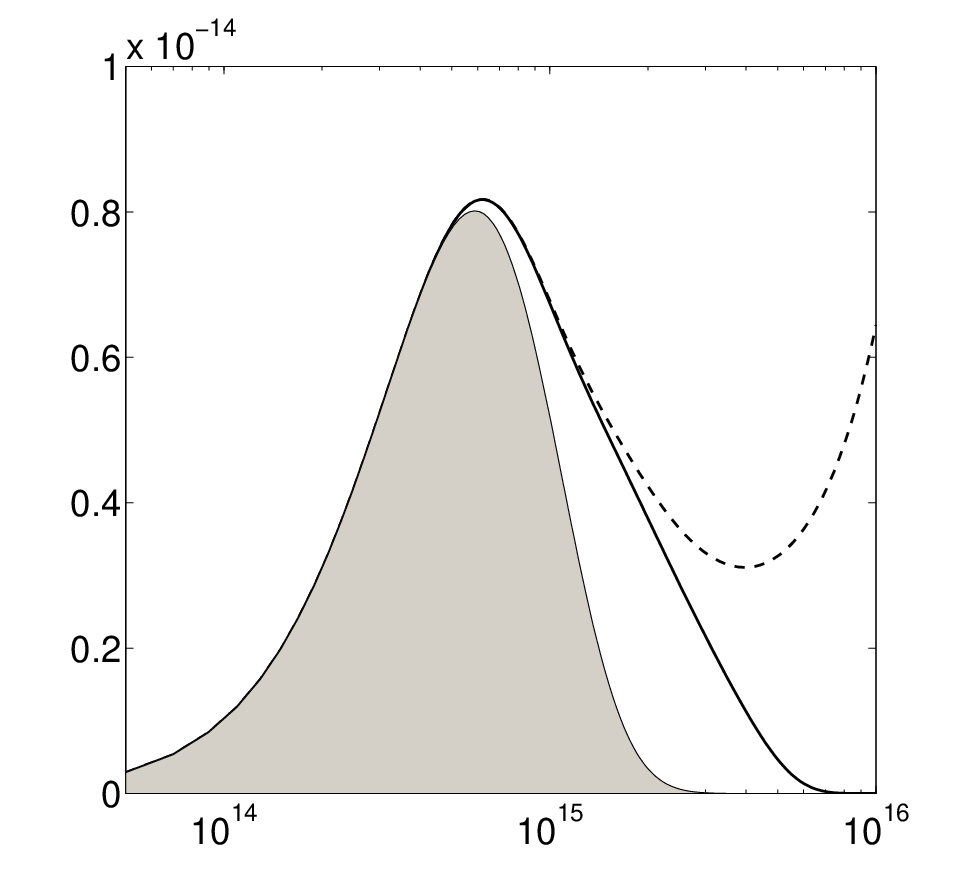
Figure 1: The shady region corresponds to the black body radiation with temperature T=1×10⁴T=1\times 10^{4} K. The solid line delimits the region of the new radiation, which is given by the deformed theory for σ=1×10⁻¹⁵\sigma=1\times 10^{-15}. The dashed line gives the radiation curves of the deformed theory with null σ\sigma. Observe that in this case, there is a divergence in the energy density at high frequencies.

In the graph of figure 1, we see the radiation curves for a temperature of 1×1041\times 10^{4} K, both for the usual black body distribution and for its deformed distribution. In the case of the deformed theory, but with σ=0\sigma=0, we clearly see a divergence in the energy density when the frequency of the radiation is increased. This is because when σ=0\sigma=0, the oscillator frequencies ωn→​(Ωn→∓π|n→|g​θ​(n)R)\omega_{\vec{n}}\left(\Omega_{\vec{n}}\mp\frac{\pi|\vec{n}|g\theta(n)}{R}\right) increase too fast, that is, like |n→|3|\vec{n}|^{3} as |n→|→∞|\vec{n}|\to\infty. For the (arbitrary) choice σ=1×10⁻¹⁵\sigma=1\times 10^{-15}m, in the figures, we see a deviation of the radiation energy density curve for the deformed theory from the usual black body radiation.
Refer to caption
Refer to caption
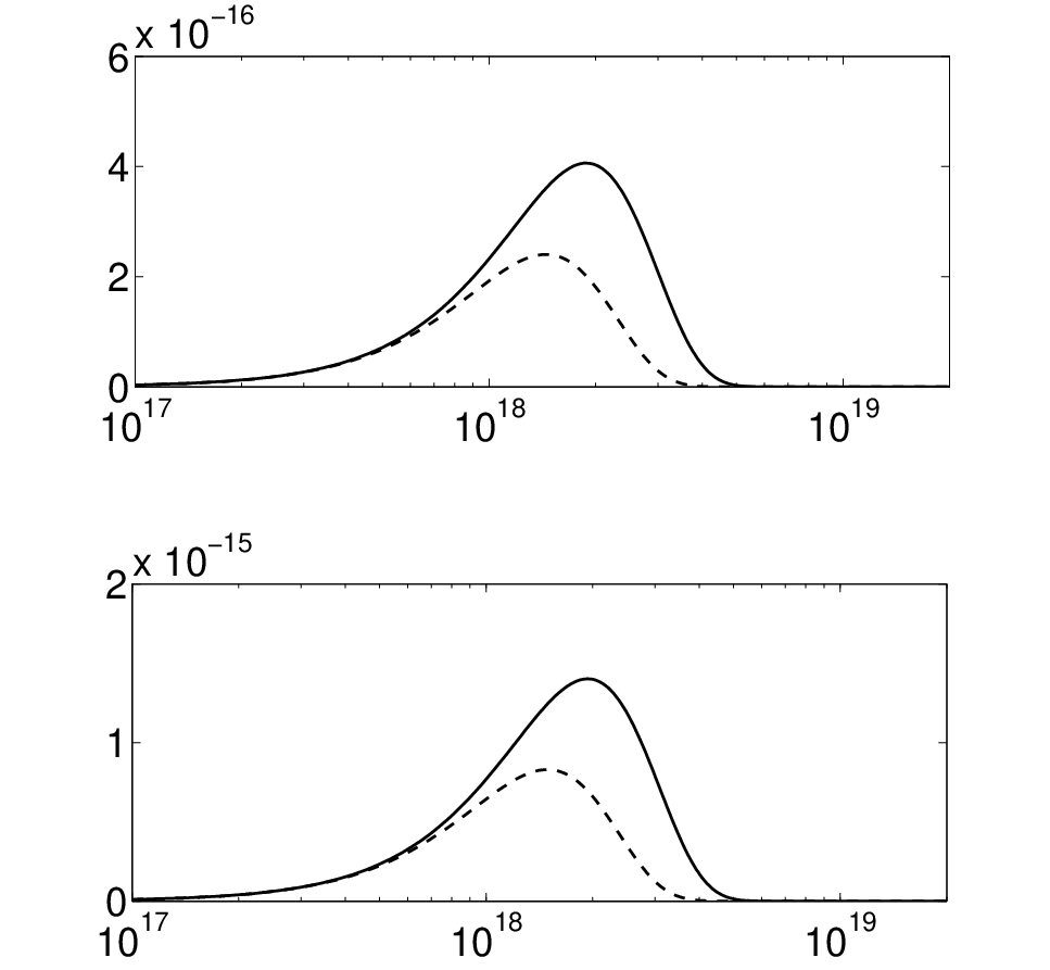
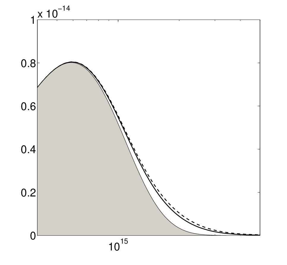
Figure 2: (a) When σ\sigma is nonnull (σ=1×10⁻¹⁵\sigma=1\times 10^{-15} and T=1×10⁴T=1\times 10^{4}K in both graphs), there exists a very small deviation with respect to the usual black body radiation at low frequencies. The graph shows the energy density curve for the new radiation with θ=1.7×10⁻¹⁴\theta=1.7\times 10^{-14} (solid line) and θ=1.9×10⁻¹⁴\theta=1.9\times 10^{-14} (dashed line);   (b) A not-so-small deviation is found for high frequencies.

The effects described above are inferred from low frequencies. The effective deviation with respect to the black body radiation is regulated by σ\sigma and θ\theta. One can see the behaviour of such deviations either in low frequencies or in high frequencies in Figure 2. In these figures the temperature is 1×1041\times 10^{4} K with fixed σ=1×10⁻¹⁸\sigma=1\times 10^{-18}m.

One can notice that for low frequencies, the effects can made very small by choosing values for the θ\theta parameter. The solid and dashed curves correspond to the values θ=1.7×10⁻¹⁴\theta=1.7\times 10^{-14} and θ=1.9×10⁻¹⁴\theta=1.9\times 10^{-14} respectively.

On the other hand, for high frequencies one can notice that a modification appears in the radiation. Such a modification is given by a peak in the radiation curve, which we refer to as the secondary peak. We observe in Figure 2 how distinct values of θ\theta lead to different values for the highest amplitude of the secondary peak.

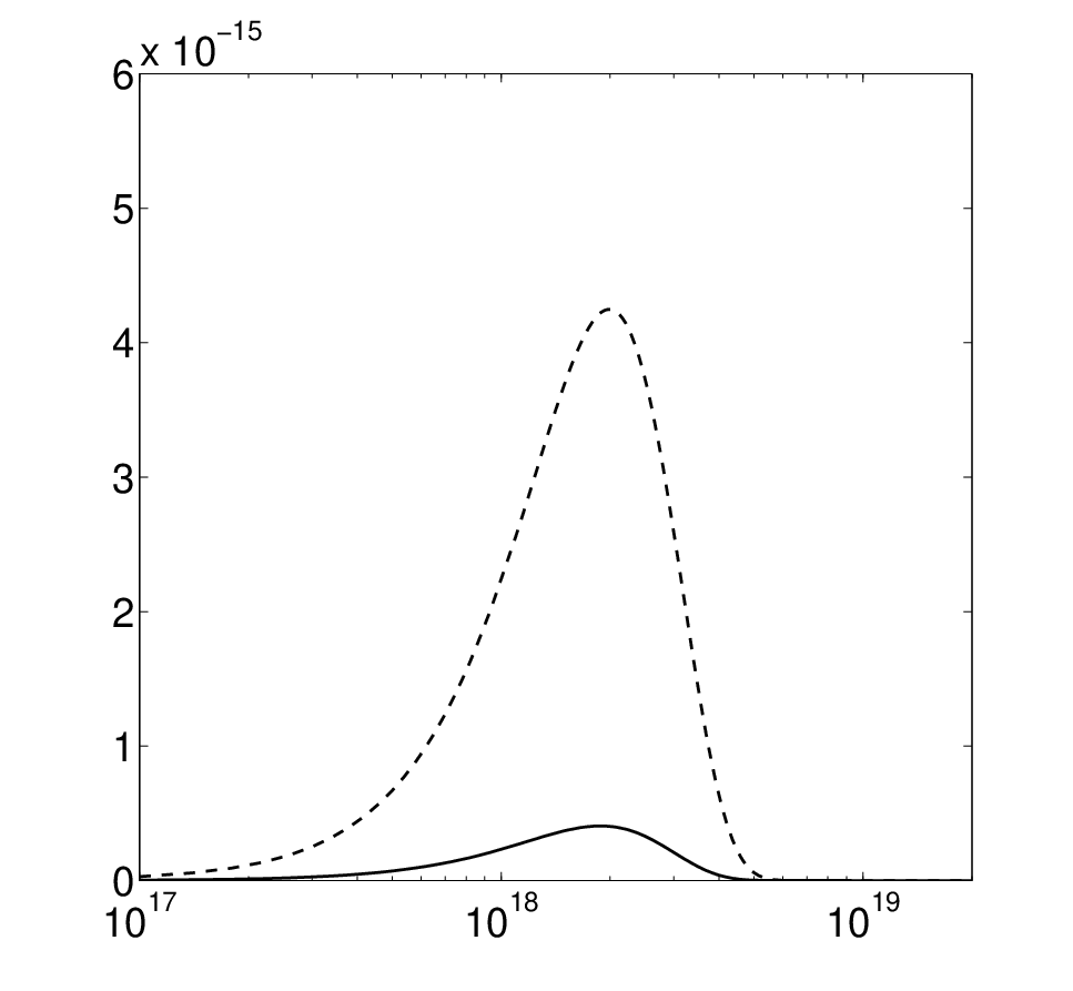
The frequency and the highest amplitude of the secondary peak are functions of the parameters. This can be seen in Figure 3. The growth of σ\sigma leads to the decrease of the highest amplitude of the modification, as well as the translation of the secondary peak to low frequencies. This agrees with the fact that when σ\sigma goes to zero, the highest amplitude grows, and the divergence appears.

One can note also in Figure 3 that as θ\theta grows, the highest amplitude of the modification grows as well. The value of θ\theta is also given by the position of the peak of the modification, however such dependence is stronger on σ\sigma than on θ\theta.

Refer to caption
Figure 3: Another example that the frequency and the highest amplitude depend on σ\sigma and θ\theta. The dependence of the highest amplitude on σ\sigma is stronger than the dependence on θ\theta. For both graphs, T=1×10⁴T=1\times 10^{4}K.

5 Conclusion

This work is based on the deformation of the target space of a field in a quantum field theory by considering the noncommutative plane ℝ2\mathbb{R}^{2} as target space. It is based on the earlier work of [10, 9]. One of the simplest of the quantum field theories, i.e., the free massless boson field theory was considered in two different cases. In the first case we recalled this theory when the base space is a cylinder S1×ℝS^{1}\times\mathbb{R}. In the second case the base space is (S1)3×ℝ(S^{1})^{3}\times\mathbb{R}.

A first consequence of such a deformation is the appearance of a term proportional to a component of angular momentum in the Hamiltonian of the theory. It affects the split of the energy levels. This split deforms the dispersion relations of the theory, which have consequences for the radiation spectrum of this theory. A new feature in our treatment is that besides the noncommutativity parameter θ\theta, we also introduce another parameter, σ\sigma, in the model, resulting in the commutation relation (24). The radiation spectrum depends on both these parameters. In order to understand its dependence on these parameters, we expanded the energy density upto second order in theta and graphically studied its dependence on the parameters. The analysis of these graphs reveals that the deviation of the new radiation spectrum with respect to the black body radiation is stronger in σ\sigma than in θ\theta.

As an application of the deformed black body spectrum, one may calculate the GZK cut-off. In [21], the GZK cut-off is calculated using the distribution of black body radiation. A follow up of the present work is to evaluate a new GZK cut-off using the deformed black body distribution obtained in this work.

Acknowledgments

The authors thank Prof. R. Abramo for pointing out that the deformed black body radiation may be relevant for the GZK cut-off. The authors also thank Prof. Y. Albuquerque for pointing out the work [21]. We also thank Prof. J. Gamboa and Prof. J. Cortez for calling our attention to [9, 10, 23, 24, 25, 26, 27, 28], which already contain many of our ideas. We have tried to acknowledge their contributions properly in the text. The work of A.P.B. is supported in part by US Department of Energy under grant number DE-FG02-85ER40231.

References

  • [1] R. Oeckl, Braided quantum field theory, Commun. Math. Phys. 217 (2001) 451–473, [hep-th/9906225].
  • [2] A. P. Balachandran, G. Mangano, A. Pinzul, and S. Vaidya, Spin and statistics on the Groenenwold-Moyal plane: Pauli- forbidden levels and transitions, Int. J. Mod. Phys. A21 (2006) 3111–3126, [hep-th/0508002].
  • [3] A. P. Balachandran, A. Pinzul, and B. A. Qureshi, UV-IR mixing in non-commutative plane, Phys. Lett. B634 (2006) 434–436, [hep-th/0508151].
  • [4] A. P. Balachandran, A. Pinzul, B. A. Qureshi, and S. Vaidya, Poincaré invariant gauge and gravity theories on the Groenewold-Moyal plane, hep-th/0608138.
  • [5] A. P. Balachandran, T. R. Govindarajan, G. Mangano, A. Pinzul, B. A. Qureshi, and S. Vaidya, Statistics and UV-IR mixing with twisted Poincaré invariance, Phys. Rev. D75 (2007) 045009, [hep-th/0608179].
  • [6] A. Pinzul, Twisted Poincaré group and spin-statistics, Int. J. Mod. Phys. A20 (2005) 6268–6277.
  • [7] G. Fiore and J. Wess, On ‘full twisted poincaré’ symmetry and qft on moyal-weyl spaces, hep-th/0701078.
  • [8] Y. Sasai and N. Sasakura, Braided quantum field theories and their symmetries, arXiv:0704.0822 [hep-th].
  • [9] J. M. Carmona, J. L. Cortes, J. Gamboa, and F. Mendez, Noncommutativity in field space and lorentz invariance violation, Phys. Lett. B565 (2003) 222–228, [hep-th/0207158].
  • [10] J. M. Carmona, J. L. Cortes, J. Gamboa, and F. Mendez, Quantum theory of noncommutative fields, JHEP 03 (2003) 058, [hep-th/0301248].
  • [11] S. Doplicher, K. Fredenhagen, and J. E. Roberts, The quantum structure of space-time at the planck scale and quantum fields, Commun. Math. Phys. 172 (1995) 187–220, [hep-th/0303037].
  • [12] J. Frohlich and K. Gawedzki, Conformal field theory and geometry of strings, hep-th/9310187.
  • [13] G. Landi, F. Lizzi, and R. J. Szabo, String geometry and the noncommutative torus, Commun. Math. Phys. 206 (1999) 603–637, [hep-th/9806099].
  • [14] N. Seiberg and E. Witten, String theory and noncommutative geometry, JHEP 09 (1999) 032, [hep-th/9908142].
  • [15] A. Y. Alekseev, A. Recknagel, and V. Schomerus, Non-commutative world-volume geometries: Branes on su(2) and fuzzy spheres, JHEP 09 (1999) 023, [hep-th/9908040].
  • [16] M. R. Douglas and N. A. Nekrasov, Noncommutative field theory, Rev. Mod. Phys. 73 (2001) 977–1029, [hep-th/0106048].
  • [17] D. Bahns, S. Doplicher, K. Fredenhagen, and G. Piacitelli, On the unitarity problem in space/time noncommutative theories, Phys. Lett. B533 (2002) 178–181, [hep-th/0201222].
  • [18] P. Aschieri, M. Dimitrijevic, F. Meyer, and J. Wess, Noncommutative geometry and gravity, Class. Quant. Grav. 23 (2006) 1883–1912, [hep-th/0510059].
  • [19] M. Chaichian, P. P. Kulish, K. Nishijima, and A. Tureanu, On a Lorentz-invariant interpretation of noncommutative space-time and its implications on noncommutative QFT, Phys. Lett. B604 (2004) 98–102, [hep-th/0408069].
  • [20] R. Oeckl, Untwisting noncommutative ℝd\mathbb{R}^{d} and the equivalence of quantum field theories, Nucl. Phys. B581 (2000) 559–574, [hep-th/0003018].
  • [21] J. Geddes, T. C. Quinn, and R. M. Wald, On the injection energy distribution of ultrahigh-energy cosmic rays, Astrophys. J. 459 (1995) 384–392, [astro-ph/9506009].
  • [22] V. P. Nair and A. P. Polychronakos, Quantum mechanics on the noncommutative plane and sphere, Phys. Lett. B505 (2001) 267–274, [hep-th/0011172].
  • [23] A. Das, J. Gamboa, F. Mendez, and J. Lopez-Sarrion, Chiral bosonization for noncommutative fields, JHEP 05 (2004) 022, [hep-th/0402001].
  • [24] J. Gamboa, J. Lopez-Sarrion, and A. P. Polychronakos, Ultraviolet modified photons and anisotropies in the cosmic microwave background radiation, Phys. Lett. B634 (2006) 471–473, [hep-ph/0510113].
  • [25] H. Falomir, J. Gamboa, J. Lopez-Sarrion, F. Mendez, and A. J. da Silva, Vortices, infrared effects and lorentz invariance violation, Phys. Lett. B632 (2006) 740–744, [hep-th/0504032].
  • [26] J. Gamboa and J. Lopez-Sarrion, U(1) noncommutative gauge fields and magnetogenesis, Phys. Rev. D71 (2005) 067702, [hep-th/0501034].
  • [27] P. Arias, J. Gamboa, J. Lopez-Sarrion, F. Mendez, and A. Das, Cpt/lorentz invariance violation and neutrino oscillation, hep-ph/0608007.
  • [28] P. Arias, H. Falomir, J. Gamboa, F. Mendez, and F. A. Schaposnik, Chiral anomaly beyond lorentz invariance, arXiv:0705.3263 [hep-th].
  • [29] A. P. Balachandran, A. M. Marques, A. R. Queiroz, and P. Teotonio-Sobrinho, Twisted Kac-Moody and Virasoro algebras, hep-th/0608081.
  • [30] V. P. Nair, Quantum mechanics on a noncommutative brane in m(atrix) theory, Phys. Lett. B505 (2001) 249–254, [hep-th/0008027].
  • [31] H. Grosse, On the construction of Möller operators for the nonlinear Schrödinger equation, Physics Letters B 86 (Oct., 1979) 267–271.
  • [32] A. B. Zamolodchikov and A. B. Zamolodchikov, Factorized s-matrices in two dimensions as the exact solutions of certain relativistic quantum field models, Annals Phys. 120 (1979) 253–291.
  • [33] L. D. Faddeev, Quantum completely integral models of field theory, Sov. Sci. Rev. C1 (1980) 107–155.
  • [34] A. P. Balachandran, S. Kurkcuoglu, and S. Vaidya, Lectures on Fuzzy and Fuzzy SUSY Physics, World Scientific Publishing Company (2007) [hep-th/0511114].