Renormalization of NN Interaction with Lorentz-invariant Chiral Two Pion Exchange.
Abstract
The renormalization of the NN interaction with the
Chiral Two Pion Exchange Potential computed using Lorentz-invariant baryon
chiral perturbation theory is considered. The short distance
singularity reduces the number of counter-terms to about a half as
those in the heavy baryon expansion. Phase shifts and deuteron
properties are evaluated and a general overall agreement is
observed.
Keywords:
NN interaction, Two Pion Exchange, Renormalization, Relativitypacs
03.65.Nk,11.10.Gh,13.75.Cs,21.30.Fe,21.45.+vI Introduction
At long distances the Nucleon-Nucleon (NN) interaction can be written as (see e.g. Brown and Jackson 1976 for a review)
| (1) |
where, and represent the One Pion Exchange (OPE) and the Two Pion Exchange (TPE) contributions to the potential, respectively. Up to power corrections in the distance , one has . Such an expansion makes sense, since there is a clear scale separation at long distances. Actually, the omitted terms in Eq. (1) represent contributions whose ranges are shorter than . These include three and higher pion exchanges, correlated meson exchanges, etc Machleidt et al. 1987. In momentum space, the expansion of Eq. (1) parallels an expansion on leading low momentum singularities, rather than a naive low momentum expansion. The systematic and model independent determination of those potentials was suggested several years ago Weinberg 1990; Ordonez and van Kolck 1992; Weinberg 1991; Ordonez et al. 1996 and pursued by many others Rijken and Stoks 1996; Kaiser et al. 1997; Friar 1999; Rentmeester et al. 1999; Entem and Machleidt 2002a (for some reviews emphasizing different viewpoints see e.g. Bedaque and van Kolck 2002; Phillips 2002; Epelbaum 2006; Rho 2006; Ruiz Arriola and Pavon Valderrama 2006 and references therein). However, in any scheme the potentials in Eq. (1) become singular at short distances, so one must truncate or renormalize the potential in a physically meaningful way in order to predict finite and unique phase shifts and deuteron properties. This has been a subject of much debate and controversy in recent times and we refer the interested reader to the literature for further details Epelbaum et al. 2000; Entem and Machleidt 2002b; Rentmeester et al. 1999; Beane et al. 2002; Entem and Machleidt 2003; Epelbaum et al. 2005; Pavon Valderrama and Ruiz Arriola 2004a; Birse and McGovern 2004; Nogga et al. 2005; Pavon Valderrama and Ruiz Arriola 2005a; Pavon Valderrama and Ruiz Arriola 2006a; Birse 2006; Pavon Valderrama and Ruiz Arriola 2006b; Pavon Valderrama and Ruiz Arriola 2007a; Epelbaum and Meissner 2006; Birse 2007.
In previous works by two of us (MPV and ERA) Pavon Valderrama and Ruiz Arriola 2005a; Pavon Valderrama and Ruiz Arriola 2006a; Pavon Valderrama and Ruiz Arriola 2006b; Pavon Valderrama and Ruiz Arriola 2007a the renormalization of NN potentials was studied using chiral potentials based on the heavy baryon formalism (HB-PT) Kaiser et al. 1997; Rentmeester et al. 1999. In the present paper, we extend those ideas to the case where Lorentz-invariant chiral potentials are used instead. In this case, the relativistic framework of baryon chiral perturbation theory (RB-PT) proposed by Becher and Leutwyler Becher and Leutwyler 1999; Becher and Leutwyler 2001 is employed in the construction of the two-pion exchange (TPE) component of the NN interaction. The remarkable difference between HB- and RB-TPE potentials lies on the long distance behavior Higa and Robilotta 2003; Higa et al. 2004; Higa 2004; Higa et al. 2005, due to the analytic structure of the scattering amplitude in the low energy region where the Mandelstam variable is close to , being the pion mass. Actually, one appealing feature of the RB-TPE potentials is that the long-distance two pion effects are correctly described, so that important contributions at the exponential level are properly re-summed, unlike its heavy baryon counterpart. In this work we are also interested on its different short distance behavior, which plays an important role on the renormalization program of the NN interaction developed in Refs. Pavon Valderrama and Ruiz Arriola 2005a; Pavon Valderrama and Ruiz Arriola 2006a; Pavon Valderrama and Ruiz Arriola 2006b; Pavon Valderrama and Ruiz Arriola 2007a. We disregard, however, explicit ’s (see e.g. Kaiser et al. 1998) and other intermediate state contributions, assuming that those degrees of freedom have been integrated out.
As we have already mentioned, the calculation of scattering and bound state properties requires specifying the NN potential at short distances, which turns out to be highly singular for the Lorentz-invariant case. Actually, a crucial issue in the present context regards the number of necessary counter-terms required by the renormalizability of the S-matrix. In the single channel situation, the results found in Refs. Pavon Valderrama and Ruiz Arriola 2005a; Pavon Valderrama and Ruiz Arriola 2006a; Pavon Valderrama and Ruiz Arriola 2006b; Pavon Valderrama and Ruiz Arriola 2007a in configuration space can be summarized as follows. If the potential is a regular one, i.e., , there is freedom to choose between the regular and irregular solution of the corresponding Schrödinger equation. In the first case the scattering length is predicted, while in the second case the scattering length becomes an input of the calculation. Singular potentials fulfill and do not allow this choice. For repulsive singular potentials [] the scattering length is predicted while for attractive singular potentials [] the scattering length must be given. The case is very special and, for , yields ultraviolet limit-cycles Beane et al. 2001; Pavon Valderrama and Ruiz Arriola 2004a; Pavon Valderrama and Ruiz Arriola 2007b. For coupled channels one must diagonalize first the coupled channel potentials and apply the single channel rules to the outgoing eigenpotentials.
In order to avoid any possible misunderstanding we hasten to emphasize that our use of the word relativistic is in a narrow sense; we are only disregarding a naive heavy baryon expansion of the virtual nucleon states in the calculation of the potential and hence taking into account important anomalous thresholds singularities Becher and Leutwyler 1999; Becher and Leutwyler 2001. This is not the same as providing a fully relativistic quantum field theoretical solution to the the two-body problem by say, solving a Bethe-Salpeter equation or any two body relativistic equation. This has always been a problem rooted in the non-perturbative divorce between crossing and unitarity in few body calculations for which the present paper has nothing to say.
The paper is organized as follows. In Sec. II we give an overview of our formalism already used in Ref. Pavon Valderrama and Ruiz Arriola 2005a; Pavon Valderrama and Ruiz Arriola 2006a; Pavon Valderrama and Ruiz Arriola 2006b; Pavon Valderrama and Ruiz Arriola 2007a. The key aspects on the derivation of the Lorentz-invariant TPE potential are briefly mentioned and the main differences with respect to the heavy baryon formalism are highlighted in Sec. III. The deuteron bound state is discussed in Sec. IV. Our predictions for phase shifts are displayed in Sec. V. Finally, in Sec. VI we draw our conclusions.
| Set | Source | |||
|---|---|---|---|---|
| Set I | Buettiker and Meissner 2000 | -0.81 | -4.69 | 3.40 |
| Set II | Rentmeester et al. 1999 | -0.76 | -5.08 | 4.70 |
| Set III | Epelbaum et al. 2004 | -0.81 | -3.40 | 3.40 |
| Set IV | Entem and Machleidt 2003 | -0.81 | -3.20 | 5.40 |
| Set | This work | -0.81 | -3.80 | 4.50 |
| Wave | NijmII (Reid93) | OPE | HB-NLO | HB-NNLO | HB-NNLO | RB-TPE |
|---|---|---|---|---|---|---|
| Set I, II & III | SetIV | |||||
| -23.727(-23.735) | Input | Input | Input | Input | Input | |
| -2.468(-2.469) | Input | — | Input | — | —(*) | |
| 2.797(2.736) | — | — | Input | — | — | |
| 1.529(1.530) | — | Input | Input | Input | Input | |
| 5.418(5.422) | Input | — | Input | Input | Input | |
| 6.505(6.453) | — | — | Input | Input | — | |
| 1.647(1.645) | — | — | Input | Input | — | |
| -1.389(-1.377) | — | Input | Input | Input | Input | |
| -7.405(-7.411) | Input | Input | Input | Input | Input | |
| -0.2844(-0.2892) | Input | Input | Input | Input | Input | |
| -0.9763(-0.9698) | — | — | Input | — | —(*) | |
| 1.609(1.600) | — | — | Input | — | —(*) | |
| 8.383(8.365) | — | — | Input | — | Input | |
| 2.703(2.686) | — | Input | Input | Input | Input | |
| -0.1449(-0.1770) | Input | — | Input | Input | Input | |
| 4.880(4.874) | — | — | Input | Input | — | |
| -9.695(-9.683) | — | — | Input | Input | — | |
| -3.229(-3.210) | — | Input | Input | Input | Input | |
| -19.17(-19.14) | Input | Input | Input | Input | Input | |
| -0.01045(-0.01053) | Input | Input | Input | Input | Input | |
| -1.250(-1.240) | — | — | Input | — | — (*) | |
| 3.609(3.586) | — | — | Input | — | — (*) | |
| 28.61(28.57) | — | — | Input | — | Input | |
| 6.128(6.082) | — | Input | Input | Input | Input | |
| -0.0090(-0.010) | Input | — | Input | Input | Input | |
| 10.68(10.66) | — | — | Input | Input | — | |
| -31.34(-31.29) | — | — | Input | Input | — |
II Formalism
Along the lines of Ref. Pavon Valderrama and Ruiz Arriola 2005a; Pavon Valderrama and Ruiz Arriola 2006a; Pavon Valderrama and Ruiz Arriola 2006b; Pavon Valderrama and Ruiz Arriola 2007a we solve the coupled channel Schrödinger equation in configuration space for the relative motion, which in compact notation reads
| (2) |
The coupled channel matrix reduced potential is defined as usual, , where is the reduced proton-neutron mass. For , can be written as
In Eq. (2) is the angular momentum, is the reduced matrix wave function and the C.M. momentum. In our case, for the spin singlet channel () and for the spin triplet channel, with , and . The potentials used in this paper were obtained in Refs. Higa and Robilotta 2003; Higa et al. 2004; Higa 2004, in coordinate space. We outline the main issues of this potential in Sec. III.
II.1 Long distance behaviour
At long distances, we assume the usual asymptotic normalization condition
| (4) |
with the coupled channel unitary S-matrix. The corresponding outgoing and incoming free spherical waves are given by
| (5) |
with the reduced Hankel functions of order , ( ), and satisfy the free Schrödinger’s equation for a free particle.
The spin singlet state () is an un-coupled state
| (6) |
while the spin triplet state () comprises one un-coupled state
| (7) |
and the two channel coupled states for which we use Stapp-Ypsilantis-Metropolis (SYM or Nuclear bar) Stapp et al. 1957 parameterization
In the present paper zero energy scattering parameters play an essential role, since they are often used (see below) as input parameters in the calculation of phase shifts. Due to unitarity of the S-matrix in the low energy limit, we have
| (14) |
with the (hermitian) scattering length matrix. The threshold behaviour of the SYM phases is
| (15) | |||||
| (16) | |||||
| (17) |
II.2 Short distance behaviour
The form of the wave functions at the origin is uniquely determined by the form of the potential at short distances (see e.g. Case 1950; Frank et al. 1971 for the case of one channel and Pavon Valderrama and Ruiz Arriola 2005a; Pavon Valderrama and Ruiz Arriola 2006a; Pavon Valderrama and Ruiz Arriola 2006b; Pavon Valderrama and Ruiz Arriola 2007a for coupled channels). For the Lorentz-invariant chiral NN potential , one has
which is a relativistic Van der Waals type force (see e.g. Feinberg et al. 1989 for the electromagnetic case). Note that this short distance behaviour without an expansion is at variance with the non-relativistic and in the standard Weinberg counting based on the HB chiral expansion. In the latter, the expansion around the limit is built in the formalism, leading to a different behavior at .
For a potential diverging at the origin as an inverse power law one has
| (18) |
with a matrix of generalized Van der Waals coefficients and . One diagonalizes the matrix by a constant unitary transformation, , yielding
| (19) |
with constants with length dimension. The plus sign corresponds to the case with a positive eigenvalue (attractive) and the minus sign to the case of a negative eigenvalue (repulsive). Then, at short distances one has the solutions
| (20) |
where for the attractive and repulsive cases one has
respectively. Here, are arbitrary short distance phases which in general depend on the energy. There are as many short distance phases as short distance attractive eigenpotentials. Orthogonality of the wave functions at the origin yield the relation
where is the number of the short distance attractive eigenpotentials. Details on the numerical implementation of these short distance boundary conditions can be looked up in Refs. Pavon Valderrama and Ruiz Arriola 2005a; Pavon Valderrama and Ruiz Arriola 2006a; Pavon Valderrama and Ruiz Arriola 2006b; Pavon Valderrama and Ruiz Arriola 2007a.
II.3 Numerical parameters
The Lorentz-invariant chiral TPE potential is specified by the pion weak decay constant , the nucleon axial coupling constant , the nucleon mass and the pion mass . In addition, at the level of approximation that we are working, it is enough to consider the low energy constants , and which characterize scattering. The corresponding RB potential is specified by the same parameters at N3LO in the HB chiral expansion.
In our numerical calculations one takes , , , in the OPE piece to account for the Goldberger-Treimann discrepancy and in the TPE piece of the potential. The corresponding pion nucleon coupling constant takes then the value , according to the Nijmegen phase shift analysis of NN scattering de Swart et al. 1997. The values of the coefficients , and used along this paper can be looked up in Table 1. There we list several Sets which have been proposed in the literature Buettiker and Meissner 2000; Rentmeester et al. 1999; Epelbaum et al. 2004; Entem and Machleidt 2003 as well as the one which will be used in the present work based on our analysis of deuteron properties below.
Renormalization requires fixing some low energy parameters while removing the cut-off. We take the values from the high quality potentials Stoks et al. 1993; Stoks et al. 1994 as have been obtained in Ref. Pavon Valderrama and Ruiz Arriola 2005b for the NijmII and Reid93 versions. We will use the Nijm II values for definiteness. As mentioned earlier, the number of independent parameters or counter-terms requires a study of the attractive/repulsive nature of the potential at short distances. The result of such an analysis for all channels considered in this work is summarized in table 2 for the different parameter sets. We also list the scattering lengths in all partial waves as determined in our previous work Pavon Valderrama and Ruiz Arriola 2005b.
III Lorentz-invariant two-pion exchange
A series of papers Higa and Robilotta 2003; Higa et al. 2004; Higa 2004; Higa et al. 2005 was devoted to the construction of the TPE component of the NN interaction, based on the Lorentz-invariant formulation of baryon chiral perturbation theory proposed by Becher and Leutwyler Becher and Leutwyler 1999; Becher and Leutwyler 2001 in their study of the system. These authors showed that it is possible to obtain a consistent power counting in a theory with a heavy particle without resorting to an integration of the heavy degrees of freedom and expansion around the limit of infinitely heavy baryon (HB-PT). The latter results can be recovered from the Lorentz-invariant formulation through an expansion in . However, this procedure destroys the correct analytic behavior of the amplitude near the low energy region close to . The underlying reason comes from the anomalous threshold of the triangle graph Becher and Leutwyler 1999 (Fig.1) right below threshold, . In the heavy baryon limit this singularity is ignored (as it collapses to the normal threshold) and any expansion of the triangle loop around this region will fail to converge. Note that the same triangle integral also appears in the TPE potential, with two pseudo-vector vertices in one nucleon and a Weinberg-Tomozawa seagull term on the other.

In order to illustrate the problem let us consider the spectral representation of the triangle graph,
| (24) |
where
| (25) |
In HB-PT the argument is assumed to be of order , yielding the expansion . The first two terms read
| (26) |
where , and and are the usual HB loop functions,
| (27) |
However, it does not take into consideration the case , when gets closer to . This region, where the naive heavy baryon expansion fails, is responsible for the long distance behavior of the triangle diagram, as can be seen by its representation in configuration space,
| (28) | |||||
Therefore it is clear that, in order to have a good asymptotic description of , one needs a decent representation for near . This is only possible if one takes the triangle anomalous threshold into account, which cannot be provided by current versions of the heavy baryon formalism.
The potential in configuration space is obtained through a Fourier transform of the potential in momentum space. There one faces the problem of non-localities, i.e., terms dependent on the variable , where and are the initial and final CM momentum of the NN system. The relativistic loop integrals, which incorporates the dynamics of the TPE, also depend on this variable in a non-trivial way. However, phenomenologically one learns that such terms are not relevant at low energies and a Taylor expansion in is usually considered11 1 For instance, in the heavy baryon potential non-localities show up only at (N3LO).. In this case the Fourier transform can be carried out in an easier way (see, for instance, Refs. Partovi and Lomon 1970; Hoshizaki and Machida 1960). Generically, in any spin-isospin channel and up to the considered order in the RB-expansion the potentials may be written as a function of at most second order in the total momentum operator. In this paper we take the local approximation on the radial part of the potentials and keep only up to linear terms in the operators. The remaining non-localities are fairly small all over the range of interest, which somehow justifies its exclusion and considerably simplifies our calculations 22 2 A rough way of estimating this in coordinate space is by acting with the operator on the local function which multiplies the variable and compare with the local which multiplies the variable . In the region between and these functions behave indeed as but the ratio between the non-local and local contribution is at the level of ..


| Set | |||||||||
| OPE | Input | 0.02634 | 0.8681(1) | 1.9351(5) | 0.2762(1) | 7.88(1)% | 0.4861(10) | 0.434(3) | |
| HB Set IV | Input | Input | 0.884(4) | 1.967(6) | 0.276(3) | 8(1)% | 0.447(5) | 0.284(8) | 0.276(13) |
| RBE Set IV | Input | 0.03198(3) | 0.8226(5) | 1.8526(10) | 0.3087(2) | 22.99(13) % | 0.5054(15) | 0.360(4) | 0.333(13) |
| RBE Set | Input | 0.02566(1) | 0.88426(2) | 1.96776(1) | 0.2749(1) | 5.59(1) % | 0.4438(3) | 0.2714(7) | 0.215(3) |
| NijmII | 0.231605 | 0.02521 | 0.8845(8) | 1.9675 | 0.2707 | 5.635% | 0.4502 | 0.2868 | |
| Reid93 | 0.231605 | 0.02514 | 0.8845(8) | 1.9686 | 0.2703 | 5.699% | 0.4515 | 0.2924 | |
| Exp. | 0.231605 | 0.0256(4) | 0.8846(9) | 1.971(6) | 0.2859(3) | 5.67(4)% | - | - | - |

IV The deuteron
In the pn CM system the deuteron wave function is
| (29) | |||||
with the total spin and and and the Pauli matrices for the proton and the neutron respectively. The functions and are the reduced S- and D-wave components of the relative wave function respectively. They satisfy the coupled set of equations in the channel
with , and the corresponding matrix elements of the coupled channel potential. We solve Eq. () together with the asymptotic condition at infinity
| (31) |
where is the deuteron wave number ( is the deuteron binding energy), is the s-wave normalization factor determined from the condition
| (32) |
and the asymptotic D/S ratio parameter is defined by . As we have mentioned already the RB-TPE potential displays a relativistic Van der Waals singularity at the origin. Thus, the discussion on whether or not the deuteron parameters and can be fixed independently on the potential depends on the short distance behaviour of the eigenvalues of the coupled channel potential matrix. As discussed in Ref. Pavon Valderrama and Ruiz Arriola 2005a; Pavon Valderrama and Ruiz Arriola 2006a; Pavon Valderrama and Ruiz Arriola 2006b; Pavon Valderrama and Ruiz Arriola 2007a also for the bound state case the number of independent parameters coincides with the number of negative (attractive) eigenpotentials at short distances. In the RB-TPE potential we are using here Higa and Robilotta 2003; Higa et al. 2004; Higa 2004 we have only one independent parameter (see table 2) which we take to be or, equivalently, the deuteron binding energy. With such a choice becomes a prediction in contrast to the HB-TPE where is an input. The outgoing deuteron wave functions are depicted in Fig. 2 for the RB-TPE potential and compared to the HB-TPE one.
Let us analyze in more detail the cut-off dependence of observables in the present RB-TPE potential. Given the fact that in the coupled channel we have one attractive and one repulsive eigenpotential at short distances we may borrow from the previous discussion on OPE Pavon Valderrama and Ruiz Arriola 2005a where we refer for further details. The practical way of introducing in this case a short distance cut-off which selects the regular solution at the origin is by appropriately choosing the auxiliary boundary condition at the point among many possible choices compatible with self-adjointness Pavon Valderrama and Ruiz Arriola 2005a. The precise choice may provide smoother limits and hence better convergence properties in the pre-asymptotic region. Actually, as we show in Appendix A, we can estimate the size of the finite cut-off corrections in deuteron observables and hence their convergence rate towards the corresponding renormalized values. The result is that up to some oscillations the convergence towards the renormalized value is exponential as , i.e. the convergence towards the renormalized value is for the RB-TPE potential ( ) as compared to for the OPE potential ( ). Here is a characteristic short distance scale of the corresponding repulsive eigenpotentials. The analysis of Appendix A also shows that, generally, the more singular the potential the faster the convergence.
For illustration purposes we show in Fig. 3 the calculated asymptotic D/S ratio of the deuteron wave function, , as a function of the short distance cut-off (in ) for the RB-TPE potential when the auxiliary boundary conditions and are considered. Note the clear and coincident plateau below for both boundary conditions following a relatively rapid variation above this region 33 3 Other auxiliary boundary conditions such as or not shown in the figure make the oscillations deduced in Appendix A more visible, but the plateau region takes place also below and yields an identical numerical result as with and .. As mentioned above, this is a typical feature of a coupled channel singular potential with one attractive and one repulsive eigenpotential which extends to all other deuteron properties. Actually, the situation strongly resembles the previously studied OPE potential which has a softer singularity at the origin Pavon Valderrama and Ruiz Arriola 2005a; the main difference is that for OPE stability takes place at a shorter scale, , than in RB-TPE potential. In the present context it is also helpful to remind that a short distance cut-off radius and a sharp momentum cut-off are inverse proportional to each other, Pavon Valderrama and Ruiz Arriola 2004b (the numerical coefficient depends on the particular regularization). Thus plotting observables as a function of enhances the finite cut-off changes while long plateaus could be observed instead as functions of . Actually, halving the short distance cut-off corresponds to doubling the momentum space cut-off. For instance, in RB (Set-) the range corresponds to the range where observables such as change less than . Pinning down this error bar would be harder if the sharp or other momentum space cut-off was used.
Our results for several deuteron properties are shown in table 3 and compared to the corresponding HB-TPE considered in our previous work Pavon Valderrama and Ruiz Arriola 2005a; Pavon Valderrama and Ruiz Arriola 2006a; Pavon Valderrama and Ruiz Arriola 2006b; Pavon Valderrama and Ruiz Arriola 2007a. Some remarks concerning the errors quoted in table 3 are in order. We provide the largest source of error in the calculation which we are able to quantify. Since we aim at renormalized results, we stop whenever the change of the cut-off causes no significant variation within a prescribed accuracy, which we take to be about an order of magnitude higher than the typical experimental or recommended value uncertainty. Thus, the cut-off range is not necessarily the same in all cases. In general terms, the more singular the potential at short distance, the faster the convergence of the result towards the renormalized limit (see e.g. Appendix A). Thus, the toughest case is OPE, where we only have singularity. Convergence in this case is the slowest, therefore shorter cut-offs are needed.


The value we obtain for for the parameter Sets of table 1 is slightly different from the experimental one, making the comparison with the HB-TPE case Pavon Valderrama and Ruiz Arriola 2006a, where was a free parameter (two attractive short distance eigenpotentials), a bit misleading. In order to obtain an accurate value of it was necessary to readjust the low energy parameters and to the values and , indeed, very similar to the values proposed by other authors Buettiker and Meissner 2000; Rentmeester et al. 1999; Epelbaum et al. 2004; Entem and Machleidt 2003 (see table 1). Actually, once we have reproduced we see a general and slight improvement in accuracy when going from the HB-TPE (where is a free parameter) of our previous work Pavon Valderrama and Ruiz Arriola 2006a to the present RB-TPE calculation (where is predicted). Basically, RB-TPE produces a sharp prediction for (with eventually no errors), whereas HB-TPE does not predict , so its experimental uncertainty propagates to other deuteron observables at about a similar level, which is still comparable or larger than the error in the quoted experimental or recommended values. The conclusion in Ref. Pavon Valderrama and Ruiz Arriola 2006a was that agreement was partly achieved because of this fuzziness in the theoretical predictions. Of course, one should not overstress the possible accuracy of the present results as regards the systematic errors; the main point of our calculation is to provide the general picture when more complete asymptotic TPE effects are correctly taken into account.




V Phase Shifts
We come to the calculation of the np phase shifts. In practice, this requires a careful wave by wave study of the renormalized limit. As can be seen in table 2, all coupled triplet channels have one attractive and one repulsive short distance eigenpotential. On the other hand, almost all singlet and uncoupled triplet channels develop an attractive singularity at short distances (sometimes depending on the parameter values). The only exceptions we found are the and channels, the latter depending on the precise values of the constants of the chiral potential. This fact determines not only the number of counterterms, but also the convergence pattern towards the renormalized result. It reaches stability for cut-offs ranging in the region , depending on the particular partial wave and also on the energy (see the discussion in the previous section IV and Appendix A). Phase shifts in coupled channels with one repulsive singular component have been computed with either auxiliary boundary conditions and for zero energy states and subsequent orthogonalization of the finite energy states by using a complementary boundary condition as described in detail in Ref. Pavon Valderrama and Ruiz Arriola 2005a for the OPE case. It is important to realize that even though renormalization requires in principle to pursue the mathematical limit , convergence is achieved in practice by length scales which are not unrealistically small and in fact are rather reasonable. This can be seen in Fig. 4 where, for illustration purposes, some selected low phases are depicted as a function of the short distance cut-off for fixed laboratory energy values. As one generally expects smaller values of are needed as the energy is increased. The approach towards the renormalized value for any partial wave depends on the attractive/repulsive character of the singular potential at short distances. So, the and channels are purely attractive and hence the finite cut-off corrections are up to oscillations Pavon Valderrama and Ruiz Arriola 2007b. On the other hand, the channel provides a repulsive case and hence finite cut-off corrections are . We remind that the smallest de Broglie wavelength probed in NN interaction below pion production threshold is . Thus, the RB-potential and the present renormalization construction also implement the desirable a priori requirement that short distance details are indeed irrelevant for the description of low energy properties.
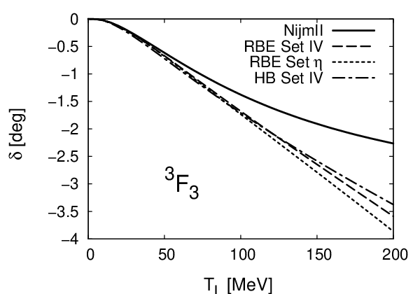
In Figs. 5 and 6 we present the np (SYM-nuclear bar) renormalized phase shifts for the total angular momentum for Spin Singlet and Uncoupled Spin Triplet and Coupled Spin Triplet channels respectively. There we compare the relativistic baryon expansion (RBE) and the heavy baryon expansion (HBE) as a function of the LAB energy compared to the Nijmegen partial wave analysis Stoks et al. 1993; Stoks et al. 1994. For definiteness we use the chiral constants , and of Ref. Entem and Machleidt 2003 (Set IV), which already provided a good description of deuteron properties after renormalization Pavon Valderrama and Ruiz Arriola 2006a at NNLO. This choice allows a more straightforward comparison to the N3LO calculation of Ref. Entem and Machleidt 2003 with finite cut-offs. We also compare with the Set which takes to the same value of and the readjusted values and based on our improved description of the deuteron in Sec. IV. Unless otherwise stated, the needed low energy parameters for these figures are always taken to be those of Ref. Pavon Valderrama and Ruiz Arriola 2005b for the NijmII potential (see Table 2). As can be clearly seen, the RB-TPE with this Set- not only improves deuteron properties but also the phase shifts all over. Again, one should not overemphasize this agreement, but it is rewarding to see that there is a general trend to stability and improvement in some channels (such as ,, ) when the RB-TPE potential is considered, while the quality of description is not worsened in other channels. At the same time one should stress, however, that generally speaking this potential needs much less counter-terms as the corresponding HB counterpart (about a half). Actually, in the Lorentz-invariant potential case one has at most one free parameter for channel as compared to the three parameters for channels in the coupled triplets. This is due to the attractive-repulsive short distance character of the coupled channel RB-TPE as compared to the attractive-attractive HB-TPE potential in these coupled channels. Again, we remind that the RB-TPE provides the correct analytic behavior of the exchange of two pions at large distances when and other excitations are not explicitly considered.
VI Conclusions
In the present paper we have analyzed the renormalization of all partial waves for NN scattering and the bound deuteron state for the Chiral Two Pion Exchange Potential computed in a relativistic baryon Expansion. Our main motivation has been to consider a potential where the asymptotic TPE effects are consistently taken care of. This gives us some confidence that long distance physics is faithfully represented by a common exponential fall-off factor . At the level of calculation considered here and other excitations are not explicitly taken into account; within a relativistic baryon expansion the contribution of this degree of freedom to the NN potential has never been computed. In addition, in the relativistic baryon expansion there appear non-local terms in the potential which involve the sum of initial and final momentum space operators which fortunately turn out to be rather small all over the range as compared to the local contributions to the potential. This simplifies the analysis tremendously since standard coordinate space methods can be used to solve the non-perturbative scattering problem and deuteron bound state and their subsequent and necessary renormalization. As we have repeatedly stressed along the paper this Lorentz-invariant potential presents a singularity at the origin which demands renormalization in order to get a finite and unique result when the TPE potential is assumed to be valid all over the range from the origin to infinity. This can be done by introducing a number of (potential independent) counter-terms and consequently physical renormalization conditions must be specified. In practice they are fixed to the values of threshold parameters, mainly scattering lengths at zero energy. Actually, we have noted that the number of necessary counter-terms is drastically reduced when the Lorentz-invariant baryon potential is compared to the heavy baryon expanded TPE potential, while both potentials are specified by the same parameters. Thus, less input is needed to predict the NN phase-shifts. Although the precise number of counter-terms depends on the parameters of the potential we find that, typically, for the channels with total angular momentum to we need 13 in the Lorentz-invariant case as compared to about 27 in the HB potential. Actually, it is noteworthy that with about a half of the counter-terms the overall agreement is improved. This is particularly striking in the and the (deuteron) channels. In other channels the improvement is moderate, indicating missing shorter range contributions to Eq. (1). Although a deeper understanding on why this dramatic reduction of the number of counter-terms happens would very helpful, and we have not attempted a large scale fit, it is very rewarding that the implementation of the correct and fairly complete long range physics deduced from One and Two Pion Exchange in conjunction with the requirement of renormalizability provides a rather reasonable description of the NN scattering data below pion production threshold.
Acknowledgements.
We would like to thank the hospitality of the European Center for Theoretical Studies on Nuclear Physics and Related Areas (ECT*) in Trento, where this work was initiated. M.P.V. also thanks W. Broniowski and P. Bożek for their kind hospitality in Krakow where part of this work has been carried out. The work of M.P.V. and E.R.A. is supported in part by funds provided by the Spanish DGI and FEDER funds with grant no. FIS2005-00810, Junta de Andalucía grants no. FQM225-05, EU Integrated Infrastructure Initiative Hadron Physics Project contract no. RII3-CT-2004-506078. The work of R.H. was supported by DOE Contract No.DE-AC05-06OR23177, under which SURA operates the Thomas Jefferson National Accelerator Facility, and by the BMBF under contract number 06BN411.Appendix A Analytical determination of finite cut-off corrections
In this appendix we determine the finite cut-off corrections to renormalized deuteron properties when the the two coupled channel potential is so that there is one attractive and one repulsive short distance eigenpotential. This is the case of OPE and RB-TPE potentials discussed in this paper. In this case it is simplest to discuss the auxiliary boundary condition
| (33) |
The analysis of other auxiliary boundary conditions such as which has actually been used in the numerical calculations is a bit messier but the final conclusion is essentially the same as with Eq. (33).
From the superposition principle of boundary conditions we may write
| (34) |
where and solve the deuteron problem, Eq. (), with the long distance boundary conditions Eq. (31) when taking and respectively. On the other hand, at short distances the coupled channel potential is diagonalized by an orthogonal transformation
| (35) |
where the mixing angle depends on the parameters of the potential only. For instance, for OPE one has , see Ref. Pavon Valderrama and Ruiz Arriola 2005a. The reduced potential behaves as
| (36) |
where and are the Van der Waals length scales associated to the repulsive and attractive channels respectively. Defining the general short distance solutions of the decoupled problems
| (37) |
where and , , , are fixed constants which depend on the potential only and may be determined by integrating in from long distances the asymptotic wave functions and . We remind that for the RB-TPE potential while for the OPE potential. Note that we must include here also the diverging exponential at the origin for the repulsive eigenpotential. The solutions at short distances behave as
| (38) |
where . Thus, using the short distance boundary condition, Eq. (33) which selects the regular solution at the origin and eventually kills the diverging exponentials when , and gathering all subsequent equations we get
| (39) | |||||
The limiting value is controlled by the short distance diverging exponentials in Eq. (37) and is given by
| (40) |
Deviations from this value for small cut-offs can be directly determined from Eq. (37) yielding
| (41) |
showing that, up to oscillations, finite cut-off corrections in the deuteron are for OPE and for RB-TPE. The generalization to other auxiliary boundary conditions and other deuteron properties is straightforward with identical result in the order of finite cut-off effects.
The case of scattering states is more tedious and will not be discussed in detail here but can also be analyzed with a combination of the coupled channel formulas of Ref. Pavon Valderrama and Ruiz Arriola 2007b (see Sect. V of that paper) and the bound state results of the present appendix. Finite cut-off effects for the S-matrix scale similarly as in the bound state case, i.e. up to oscillations they are for OPE and for RB-TPE.
References
- Brown and Jackson (1976) G. Brown and A. D. Jackson, The Nucleon-Nucleon Interaction (North-Holland Publishing Company. Amsterdam, 1976).
- Machleidt et al. (1987) R. Machleidt, K. Holinde, and C. Elster, Phys. Rept. 149, 1 (1987).
- Weinberg (1990) S. Weinberg, Phys. Lett. B251, 288 (1990).
- Ordonez and van Kolck (1992) C. Ordonez and U. van Kolck, Phys. Lett. B291, 459 (1992).
- Weinberg (1991) S. Weinberg, Nucl. Phys. B363, 3 (1991).
- Ordonez et al. (1996) C. Ordonez, L. Ray, and U. van Kolck, Phys. Rev. C53, 2086 (1996), eprint hep-ph/9511380.
- Rijken and Stoks (1996) T. A. Rijken and V. G. J. Stoks, Phys. Rev. C54, 2851 (1996), eprint nucl-th/9509029.
- Kaiser et al. (1997) N. Kaiser, R. Brockmann, and W. Weise, Nucl. Phys. A625, 758 (1997), eprint nucl-th/9706045.
- Friar (1999) J. L. Friar, Phys. Rev. C60, 034002 (1999), eprint nucl-th/9901082.
- Rentmeester et al. (1999) M. C. M. Rentmeester, R. G. E. Timmermans, J. L. Friar, and J. J. de Swart, Phys. Rev. Lett. 82, 4992 (1999), eprint nucl-th/9901054.
- Entem and Machleidt (2002a) D. R. Entem and R. Machleidt, Phys. Rev. C66, 014002 (2002a), eprint nucl-th/0202039.
- Bedaque and van Kolck (2002) P. F. Bedaque and U. van Kolck, Ann. Rev. Nucl. Part. Sci. 52, 339 (2002), eprint nucl-th/0203055.
- Phillips (2002) D. R. Phillips, Czech. J. Phys. 52, B49 (2002), eprint nucl-th/0203040.
- Epelbaum (2006) E. Epelbaum, Prog. Part. Nucl. Phys. 57, 654 (2006), eprint nucl-th/0509032.
- Rho (2006) M. Rho (2006), eprint nucl-th/0610003.
- Ruiz Arriola and Pavon Valderrama (2006) E. Ruiz Arriola and M. Pavon Valderrama (2006), eprint nucl-th/0609080.
- Epelbaum et al. (2000) E. Epelbaum, W. Gloeckle, and U.-G. Meissner, Nucl. Phys. A671, 295 (2000), eprint nucl-th/9910064.
- Entem and Machleidt (2002b) D. R. Entem and R. Machleidt, Phys. Lett. B524, 93 (2002b), eprint nucl-th/0108057.
- Beane et al. (2002) S. R. Beane, P. F. Bedaque, M. J. Savage, and U. van Kolck, Nucl. Phys. A700, 377 (2002), eprint nucl-th/0104030.
- Entem and Machleidt (2003) D. R. Entem and R. Machleidt, Phys. Rev. C68, 041001 (2003), eprint nucl-th/0304018.
- Epelbaum et al. (2005) E. Epelbaum, W. Glockle, and U.-G. Meissner, Nucl. Phys. A747, 362 (2005), eprint nucl-th/0405048.
- Pavon Valderrama and Ruiz Arriola (2004a) M. Pavon Valderrama and E. Ruiz Arriola, Phys. Rev. C70, 044006 (2004a), eprint nucl-th/0405057.
- Birse and McGovern (2004) M. C. Birse and J. A. McGovern, Phys. Rev. C70, 054002 (2004), eprint nucl-th/0307050.
- Nogga et al. (2005) A. Nogga, R. G. E. Timmermans, and U. van Kolck, Phys. Rev. C72, 054006 (2005), eprint nucl-th/0506005.
- Pavon Valderrama and Ruiz Arriola (2005a) M. Pavon Valderrama and E. Ruiz Arriola, Phys. Rev. C72, 054002 (2005a), eprint nucl-th/0504067.
- Pavon Valderrama and Ruiz Arriola (2006a) M. Pavon Valderrama and E. Ruiz Arriola, Phys. Rev. C74, 054001 (2006a), eprint nucl-th/0506047.
- Birse (2006) M. C. Birse, Phys. Rev. C74, 014003 (2006), eprint nucl-th/0507077.
- Pavon Valderrama and Ruiz Arriola (2006b) M. Pavon Valderrama and E. Ruiz Arriola, Phys. Rev. C74, 064004 (2006b), eprint nucl-th/0507075.
- Pavon Valderrama and Ruiz Arriola (2007a) M. Pavon Valderrama and E. Ruiz Arriola, Phys. Rev. C75, 059905(E) (2007a).
- Epelbaum and Meissner (2006) E. Epelbaum and U. G. Meissner (2006), eprint nucl-th/0609037.
- Birse (2007) M. C. Birse (2007), eprint arXiv:0706.0984 [nucl-th].
- Becher and Leutwyler (1999) T. Becher and H. Leutwyler, Eur. Phys. J. C9, 643 (1999), eprint hep-ph/9901384.
- Becher and Leutwyler (2001) T. Becher and H. Leutwyler, JHEP 06, 017 (2001), eprint hep-ph/0103263.
- Higa and Robilotta (2003) R. Higa and M. R. Robilotta, Phys. Rev. C68, 024004 (2003), eprint nucl-th/0304025.
- Higa et al. (2004) R. Higa, M. R. Robilotta, and C. A. da Rocha, Phys. Rev. C69, 034009 (2004), eprint nucl-th/0310011.
- Higa (2004) R. Higa (2004), eprint nucl-th/0411046.
- Higa et al. (2005) R. Higa, M. R. Robilotta, and C. A. da Rocha (2005), eprint nucl-th/0501076.
- Kaiser et al. (1998) N. Kaiser, S. Gerstendorfer, and W. Weise, Nucl. Phys. A637, 395 (1998), eprint nucl-th/9802071.
- Beane et al. (2001) S. R. Beane et al., Phys. Rev. A64, 042103 (2001), eprint quant-ph/0010073.
- Pavon Valderrama and Ruiz Arriola (2007b) M. Pavon Valderrama and E. Ruiz Arriola (2007b), eprint arXiv:0705.2952 [nucl-th].
- Buettiker and Meissner (2000) P. Buettiker and U.-G. Meissner, Nucl. Phys. A668, 97 (2000), eprint hep-ph/9908247.
- Epelbaum et al. (2004) E. Epelbaum, W. Gloeckle, and U.-G. Meissner, Eur. Phys. J. A19, 401 (2004), eprint nucl-th/0308010.
- Stoks et al. (1994) V. G. J. Stoks, R. A. M. Klomp, C. P. F. Terheggen, and J. J. de Swart, Phys. Rev. C49, 2950 (1994), eprint nucl-th/9406039.
- Pavon Valderrama and Ruiz Arriola (2005b) M. Pavon Valderrama and E. Ruiz Arriola, Phys. Rev. C72, 044007 (2005b).
- Stapp et al. (1957) H. P. Stapp, T. J. Ypsilantis, and N. Metropolis, Phys. Rev. 105, 302 (1957).
- Case (1950) K. M. Case, Phys. Rev. 80, 797 (1950).
- Frank et al. (1971) W. Frank, D. J. Land, and R. M. Spector, Rev. Mod. Phys. 43, 36 (1971).
- Feinberg et al. (1989) G. Feinberg, J. Sucher, and C. K. Au, Phys. Rept. 180, 83 (1989).
- de Swart et al. (1997) J. J. de Swart, M. C. M. Rentmeester, and R. G. E. Timmermans, PiN Newslett. 13, 96 (1997), eprint nucl-th/9802084.
- Stoks et al. (1993) V. G. J. Stoks, R. A. M. Kompl, M. C. M. Rentmeester, and J. J. de Swart, Phys. Rev. C48, 792 (1993).
- Partovi and Lomon (1970) M. H. Partovi and E. L. Lomon, Phys. Rev. D2, 1999 (1970).
- Hoshizaki and Machida (1960) N. Hoshizaki and S. Machida, Prog. Theor. Phys. 24, 1325 (1960).
- de Swart et al. (1995) J. J. de Swart, C. P. F. Terheggen, and V. G. J. Stoks (1995), eprint nucl-th/9509032.
- Pavon Valderrama and Ruiz Arriola (2004b) M. Pavon Valderrama and E. Ruiz Arriola (2004b), eprint nucl-th/0410020.