Two-parameter scaling of correlation functions near continuous phase transitions

Correlation functions in the vicinity of continuous phase transitions usually assume a scaling form at long wavelengths.Ma73; Fisher74 Asymptotically, for wave-vectors $k$ much smaller than the relevant microscopic scale $\Lambda_{0}$ (such as the inverse lattice spacing), the order parameter correlation function $G(k)$ can be written as $G(k)=k^{-2+\eta}g^{\pm}(k\xi)$, where the anomalous dimension $\eta$ characterizes the universality class of the system, $\xi$ is the order parameter correlation length, and the scaling functions $g^{+}(x)$ and $g^{-}(x)$ describe the regime above and below the critical temperature $T_{c}$, respectively. Precisely at the temperature $T=T_{c}$ there should be a unique scaling function, so that $g^{+}(\infty)=g^{-}(\infty)$. If the dimensionality $D$ of the system is smaller than its upper critical dimension, then $g^{\pm}(x)$ approach finite limits for large $\Lambda_{0}\xi$ and we may take the limit $\Lambda_{0}\rightarrow\infty$. According to the single-parameter scaling hypothesis, the functions $g^{\pm}(x)$ are essentially determined by their asymptotic limits for small and large $x$, so that an extrapolation to the crossover regime $x\approx 1$ is possible either from the region $x\gg 1$, or from $x\ll 1$. However, it is clear that another prominent scale, which is deducible already from a dimensional analysis of Ginzburg-Landau-type theories but is absent from the one-parameter-scaling picture, will be important at larger wavevectors: the interaction-dependent scale $k_{c}$ which measures the size of the Ginzburg critical region.Amit74 Here we shall assume a microscopic model such that the scale $k_{c}$ is small compared to the natural cutoff of the model. This happens e. g. for Ising models if the range of interactions is made very large Kim03 or near the critical point of complex fluids.Anisimov05 In these systems a classical-to-critical crossover can be observed from a region dominated by the Gaussian fixed point to the region governed by the Wilson-Fisher fixed point. While the crossover of static thermodynamic derivates have been well studied in the past,Anisimov95; Binder00; Kim03; Anisimov05 the crossover behavior of the order parameter correlation function has only been investigated within a one-parameter theory valid right at $T_{c}$.Baym99; Ledowski04; BlaizotI05

In this work we extend the one-parameter scaling theory for correlation functions to account also for the interaction-dependent scale $k_{c}\ll\Lambda_{0}$ which divides the critical regime $\xi^{-1}\ll k\ll\Lambda_{0}$ into two separate regimes where $G(k)$ has rather different properties:Baym99; Ledowski04; BlaizotI05 only in the critical long-wavelength (CL) regime $\xi^{-1}\ll k\ll k_{c}\ll\Lambda_{0}$ does the correlation function scale asymptotically with an anomalous dimension $\eta$. For $k_{c}\xi\gg 1$ there exists another critical short-wavelength (CS) regime $\xi^{-1}\ll k_{c}\ll k\ll\Lambda_{0}$ where the behavior of $G(k)$ is still universal but distinct from the anomalous scaling in the CL regime. The scale $k_{c}$ is present in the usual renormalization group (RG) analysis, Anisimov95 but is lost if the RG flow is linearized in the vicinity of the critical fixed point.

Taking into account the macroscopically ordered and disordered regimes, four different macroscopic domains of wave-vectors should be distinguished, as summarized in Fig. 1.

In order to bring out the difference between the CL and the CS regime, we express $G(k)$ in terms of the irreducible self-energy $\Sigma(k)=G^{-1}(k)-{k}^{2}$. In the CL regime $\Sigma(k)$ scales asymptotically as $k^{2-\eta}$ which dominates the bare $k^{2}$-dispersion, so that $G(k)\approx[\Sigma(k)]^{-1}$. On the other hand, in the CS regime $\Sigma(k)$ may or may not be larger than $k^{2}$, depending on the strength of the interaction. What is more important here is that for $k_{c}\ll k\ll\Lambda_{0}$ the self-energy can still be expressed in terms of a universal scaling function which shows power law behavior different from the CL regime. Therefore, the self-energy in the macroscopic domain $k\ll\Lambda_{0}$ should be written in terms of scaling functions $\sigma^{\pm}(x,y)$ depending on two parameters $x=k\xi$ and $y=k/k_{c}$,

where $\sigma^{+}(x,y)$ corresponds to the disordered phase $T>T_{c}$, while $\sigma^{-}(x,y)$ describes the ordered phase $T<T_{c}$. If the system is cooled through $T_{c}$ and one probes the system at a fixed scale $k$, then the asymptotic critical behavior with anomalous exponent $\eta$ can only be observed in the CL regime $\xi^{-1}\ll k\ll k_{c}$. Yet, the same experiment at $k_{c}\ll k$ would reveal the universal behavior of the self-energy in the CS regime. The non-universal scale $k_{c}$, defining the width of the CL regime, is missed within the field-theoretical renormalization group, which effectively sets $k_{c}=\infty$ in the self-energy. However, $k_{c}$ and the scaling functions $\sigma^{\pm}(x,y)$ can be calculated using the functional renormalization group.Wetterich93; Morris94; Berges02; Ledowski04; Schuetz06

We believe that the statements above are general and apply to any continuous phase transition. In the rest of this work we shall demonstrate their validity by an approximate calculation of the scaling functions $\sigma^{\pm}(x,y)$ for the Ising universality class in $D$ dimensions, which can be modeled by an action involving a real field $\varphi(\bm{r})$,

where an ultraviolet (UV) cutoff $\Lambda_{0}$ is assumed to regularize the theory. It is instructive to consider first the perturbative calculation of the self-energy, which is possible as long as the relevant dimensionless coupling constant $\bar{u}_{0}=u_{\Lambda_{0}}\xi^{4-D}$ is small. The correlation length $\xi$ can be expressed in terms of the self-energy as $\xi^{-2}=Z\Sigma(0)$, where the field renormalization factor $Z$ is defined as $Z^{-1}=1+\partial\Sigma(k)/\partial k^{2}|_{k=0}$. For $D<4$, i.e. below the upper critical dimension of our model, the loop integrals generated in the perturbative expansion are UV convergent and we may take the limit $\Lambda_{0}\rightarrow\infty$. Perturbation theory yields the self-energy in scaling form, $\xi^{2}\Sigma(k)=Z^{-1}+\Delta\sigma_{0}^{\pm}(k\xi)$. The lowest order diagrams giving rise to a momentum dependence of the self-energy are shown in Fig. 2. In the disordered phase the corresponding scaling function is (up to order $O(\bar{u}_{0}^{3})$)

where $\bm{n}$ is an arbitrary unit vector, $\int_{\bm{p}}=\int\frac{d^{D}p}{(2\pi)^{D}}$, and $\chi(p)=\int_{\bm{p}^{\prime}}\big([\bm{p}^{\prime 2}+1][(\bm{p}^{\prime}+\bm{p}\big)^{2}+1])^{-1}$. For $T<T_{c}$ there is a finite three-legged vertex of order $\bar{u}_{0}^{1/2}$, so that the leading momentum dependent contribution to the scaling function $\Delta\sigma_{0}^{-}(x)$ is given by the lower diagram in Fig. 2 which is linear in $\bar{u}_{0}$,

An explicit evaluation of $\Delta\sigma_{0}^{\pm}(x)$ in $D=3$ is shown in Fig. 2. The qualitative behavior of the functions $\sigma^{\pm}(x)$ is easily obtained for arbitrary $D$. While $\Delta\sigma_{0}^{\pm}(x)\propto x^{2}$ for $x\rightarrow 0$, the asymptote for large $x$ is non-trivial due to the non-analytic behavior of the function $\chi(q)\propto q^{D-4}$ for large $q$ in $D<4$. We find $\Delta\sigma_{0}^{+}(x)\propto x^{2(D-3)}$ for $3<D<4$, $\Delta\sigma_{0}^{+}(x)\propto\ln x$ for $D=3$, and $\Delta\sigma_{0}^{+}(x)\sim\Delta\sigma_{0}^{+}(\infty)=O(1)$ for $2<D<3$. In the ordered phase, the scaling function $\Delta\sigma_{0}^{-}(x)$ approaches for large $x$ a finite limit $\Delta\sigma_{0}^{-}(\infty)=\frac{3}{2}\bar{u}_{0}\chi(0)$ but the sub-leading correction is non-analytic, $\Delta\sigma_{0}^{-}(x)-\Delta\sigma_{0}^{-}(\infty)\propto x^{D-4}$.

Lowest order perturbation theory does not directly reveal the existence of a second characteristic length scale $k_{c}^{-1}$ besides $\xi$. However, the perturbative approach breaks down in the vicinity of the critical point for $D<4$ since the effective dimensionless expansion parameter $\bar{u}_{0}=u_{\Lambda_{0}}\xi^{4-D}$ diverges. A consistent resummation of these divergences using a RG approach not only leads to non-trivial renormalization of $\xi$, but also reveals the presence of the characteristic scale $k_{c}$.Ledowski04 The signature of both scales $k_{c}$ and $\xi^{-1}$ is already visible in the usual one-loop RG equations for the rescaled coupling parameters ${r}_{l}=Z_{l}r_{\Lambda}/\Lambda^{2}$ and ${u}_{l}=K_{D}Z_{l}^{2}\Lambda^{D-4}u_{\Lambda}$, describing the evolution of $r_{\Lambda}$ and $u_{\Lambda}$ in Eq. (2) as the degrees of freedom in the momentum shell $\Lambda=\Lambda_{0}e^{-l}<k<\Lambda_{0}$ are integrated out.Ma73; Fisher74 Here, $Z_{l}$ is a field renormalization factor and $K_{D}=2^{1-D}\pi^{-D/2}/\Gamma(D/2)$. For $T>T_{c}$ the one-loop RG equations are Ma73

If we fine-tune the initial value ${r}_{0}$ such that the system is close to the critical point, the typical RG flow of ${r}_{l}$ and ${u}_{l}$ as a function of the “RG time” $l$ is shown in Fig. 3.

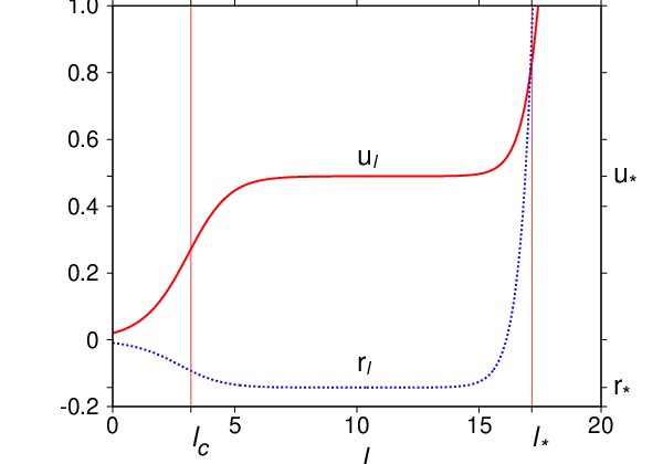
The two characteristic RG times $l_{c}$ and $l_{\ast}$ clearly separate three distinct regimes. In the regime $0<l\lesssim l_{c}$, the coupling parameters ${r}_{l}$ and ${u}_{l}$ flow toward the values ${r}_{\ast}$ and ${u}_{\ast}$ associated with the critical fixed point; in the intermediate interval $l_{c}\lesssim l\lesssim l_{\ast}$ the RG flow is close to the fixed point and very slow while for $l_{\ast}\lesssim l$ the trajectory rapidly flows away from the fixed point. A simple calculation Ledowski04 yields the estimate $l_{c}\approx(4-D)^{-1}\ln({u}_{\ast}/{u}_{0})$ for ${u}_{0}\ll{u}_{\ast}$. The one-parameter scaling hypothesis is based on the analysis of the linearised RG flow in the vicinity of the fixed point and correlates with the existence of only one unstable direction. The eigenvalue corresponding to the unstable direction then directly determines the scaling of $\xi$, see e. g. Refs. [Ma73; Fisher74]. The underlying assumption is that as long as the initial parameters are close to the critical surface (not necessarily close to the fixed point), the unstable direction will completely dominate the flow and thus the behavior at small $k$. Corrections to pure scaling are known to arise, if the stable (i.e. irrelavant) directions of the linearised flow are also accounted for.Fisher74; Wegner72 However, the analysis leading to one-parameter scaling is incomplete since the flow on the critical surface itself will typically introduce (at least) one additional scale which is not visible in the linearized flow. This is how the characteristic size $k_{c}$ of the Ginzburg critical region enters and how the one-parameter scaling hypothesis can be extended.Anisimov95 Below, we show that the RG times $l_{c}$ and $l_{\ast}$ and the associated scales $k_{c}=\Lambda_{0}e^{-l_{c}}$ and $\xi^{-1}=\Lambda_{0}e^{-l_{\ast}}$ separate regimes where the momentum dependent self-energy shows qualitatively different behavior.

To obtain the self-energy in the vicinity of the critical point taking into account the full RG flow we use the functional renormalization group (FRG).Wetterich93; Morris94; Berges02; Ledowski04; Schuetz06 An exact hierarchy of flow equations for the one-line irreducible vertices of our model is obtained by differentiating the corresponding generating functional with respect to $\Lambda$ and then expanding this functional in powers of the fields.Morris94; Schuetz06 The true self-energy is then obtained as $\Sigma(k)=\lim_{\Lambda\rightarrow 0}\Sigma_{\Lambda}(k)$. To calculate the scaling functions defined in Eq. (1), it is convenient to work with rescaled variables which manifestly exhibit the scaling dimensions of all parameters. With dimensionless momenta $\bm{q}=\bm{k}/\Lambda$ we define the dimensionless self-energy as $\Gamma_{l}(q)=Z_{l}\Lambda^{-2}\Sigma_{\Lambda}(\Lambda q)$, where $l=-\ln(\Lambda/\Lambda_{0})$. It satisfies an exact flow equation of the form Ledowski04

where $\eta_{l}=-\partial_{l}\ln Z_{l}=\partial\dot{\Gamma}_{l}(q)/\partial q^{2}|_{q=0}$ is the flowing anomalous dimension. The function $\dot{\Gamma}_{l}(q)$ depends on higher order irreducible vertices and describes the usual mode elimination step of the RG procedure. A graphical representation of the interaction processes contained in $\dot{\Gamma}_{l}(q)$ is shown in Fig. 4. Note that in the ordered phase, where our field has a finite vacuum expectation value $\langle\varphi_{\bm{k}}\rangle=(2\pi)^{D}\delta(\bm{k})M_{\Lambda}$, Eq. (7) has to be augmented by a flow equation for the flowing order parameter $M_{\Lambda}$, which is obtained by requiring that the vertex with one external leg vanishes identically for all $\Lambda$.Schuetz06

Defining $\dot{\gamma}_{l}(q)=\dot{\Gamma}_{l}(q)-\dot{\Gamma}_{l}(0)$, the physical self-energy can be written as an integral over the entire RG trajectory,

To relate this to the scaling functions $\sigma^{\pm}(x,y)$ defined in Eq. (1), we use the definitions $k_{c}=\Lambda_{0}e^{-l_{c}}$, $x=k\xi$, $y=k/k_{c}$. By construction $e^{-2l_{\ast}}=(\Lambda_{0}\xi)^{-2}=\lim_{l\rightarrow\infty}e^{-2l}{r}_{l}$ and $x/y=(k_{c}\xi)=e^{l_{\ast}-l_{c}}$. Our final result is

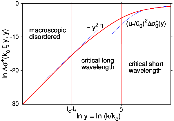
The corresponding scaling form of the order parameter correlation function is $G(k)=k_{c}^{-2}g^{\pm}(k\xi,k/k_{c})$, with $g^{\pm}(x,y)=[y^{2}+\sigma^{\pm}(x,y)]^{-1}$. The behavior of $g^{\pm}(x,y)$ crucially depends of the ratio $y/x$. Exactly at the critical point one has $x=\infty$, so that $\sigma_{\ast}(y)=\sigma^{\pm}(\infty,y)$. In the CL regime $y\ll 1$ we obtain the usual anomalous scaling $\sigma_{\ast}(y)\propto y^{2-\eta}$, while in the CS regime $y\gg 1$ $\sigma_{\ast}(y)\propto\ln y$ in $D=3$, which resembles the perturbative result $(u_{*}/\bar{u}_{0})^{2}\Delta\sigma_{0}^{+}(k/k_{c})$ shown in Fig. 2 where $k_{c}$ now plays the role of an effective infrared cutoff.Baym99

Away from criticality, Eq. (9) can only be evaluated numerically. The result of a calculation of $\sigma^{+}(x,y)$ for our model in $D=3$, using a similar truncation of the FRG flow equations as in Ref. Ledowski04, is shown in Fig. 5; the crossover between the different regimes is clearly visible.

A FRG calculation of $\sigma^{-}(x,y)$, using the flow equations for the irreducible vertices in the ordered phase derived in Ref. [Schuetz06], will be given elsewhere.Sinner07 In the regime $y\gg x$, which corresponds to $k_{c}\ll\xi^{-1}$, the system is far away from criticality (see Fig. 1), and the scale $k_{c}$ disappears from the problem. In this case it is better to normalize the self-energy differently,

Evaluating this expression to lowest order in the interaction using the trivial scaling ${r}_{l}\approx e^{2l}r_{l=0}$ and ${u}_{l}\approx e^{(4-D)l}u_{l=0}$, the second term on the right-hand side reduces for $T>T_{c}$ to the function $\Delta\sigma_{0}^{+}(x)$ given in Eq. (3) and for $T<T_{c}$ to the function $\Delta\sigma_{0}^{-}(x)$ given in Eq. (4).

In summary, we argue that the correlation function $G(k)$ near continuous phase transitions has a scaling form which involves (at least) two parameters. While in the critical long wavelength (CL) regime the self-energy shows asymptotically the usual anomalous scaling, $\Sigma(k)\propto k^{2-\eta}$, there exists another macroscopic critical short-wavelength (CS) regime $k_{c}\ll k\ll\Lambda_{0}$ where the scaling of the self-energy is given by a different power law. The scaling function describes the crossover between these regimes and the macroscopically ordered and disordered regime, as well as the finite-$k$ corrections to the asymptotic $k^{2-\eta}$ behavior (which is reached only for $k\to 0$) in the CL regime. The non-universal scale $k_{c}$ derives from the nonlinear behavior of the RG flow on the critical surface and is missed if the flow is linearized around the critical fixed point. Although for concreteness we have focused here on the Ising universality class, the two parameter scaling applies to the critical behavior of systems which in the continuum limit are well described by a Ginzburg-Landau-type action in which terms which are higher order than quartic in the fields are negligible. The CS regime $k_{c}\ll k\ll\Lambda_{0}$ is accessible only if $k_{c}$ is small compared with the effective UV cutoff $\Lambda_{0}$. For the case of generalized Ising-models, this requires that the range of interacions is very large.Kim03; Binder00 A similar crossover might be more readily observed in near-critical polymer solutions where the crossover scale depends on the radius of gyration of the polymer Anisimov05; Binder00 which can be very large.

We thank E. Vicari and A. Pelissetto for interesting and useful correspondence.

References

- (1) S. K. Ma, Rev. Mod. Phys. 45, 589 (1973).
- (2) M. E. Fisher, Rev. Mod. Phys. 46, 597 (1974).
- (3) D. J. Amit, J. Phys. C 7, 3369 (1974).
- (4) M. A. Anisimov, A. A. Povodyrev, V. D. Kulikov, and J. V. Sengers, Phys. Rev. Lett. 75, 3146 (1995); A. Pelissetto and E. Vicari, Phys. Rep. 368, 549 (2002); C. Bagnuls and C. Bervillier, Phys. Rev. E 65, 066132 (2002).
- (5) K. Binder, E. Luijte, M. Müller, N. B. Wilding, and H. W. J. Blöte, Physica A 281, 112 (2000).
- (6) Y. C. Kim, M. A. Anisimov, J. V. Sengers, and E. Luijten, J. Stat. Phys. 110, 591 (2003).
- (7) M. A. Anisimov, A. F. Kostko, J. V. Sengers, and I. K. Yudin, J. Chem. Phys. 123, 164901 (2005).
- (8) G. Baym, J.-P. Blaizot, M. Holzmann, F. Laloë, and D. Vautherin, Phys. Rev. Lett. 83, 1703 (1999); G. Baym, J.-P. Blaizot, and J. Zinn-Justin, Europhys. Lett. 49, 150 (2000).
- (9) S. Ledowski, N. Hasselmann, and P. Kopietz, Phys. Rev. A 69, 061601(R) (2004); N. Hasselmann, S. Ledowski, and P. Kopietz, ibid. 70, 063621 (2004).
- (10) J.-P. Blaizot, R. Mendez-Galain, and N. Wschebor, Phys. Rev. E 74 051116 (2006).
- (11) B. I. Halperin and P. C. Hohenberg, Phys. Rev. 177, 952 (1968).
- (12) C. Wetterich, Phys. Lett. B 301, 90 (1993).
- (13) T. R. Morris, Int. J. Mod. Phys. A 9, 2411 (1994).
- (14) J. Berges, N. Tetradis, and C. Wetterich, Phys. Rep. 363, 223 (2002).
- (15) F. Schütz and P. Kopietz, J. Phys. A: Math. Gen. 39, 8205 (2006).
- (16) F. J. Wegner, Phys. Rev. B 5, 4529 (1972).
- (17) A. Sinner, N. Hasselmann, and P. Kopietz, arXiv:0707.4110.