The Standard Model of Electroweak Interactions
Abstract
Gauge invariance is a powerful tool to determine the dynamics of the electroweak and strong forces. The particle content, structure and symmetries of the Standard Model Lagrangian are discussed. Special emphasis is given to the many phenomenological tests which have established this theoretical framework as the Standard Theory of electroweak interactions.
1 Introduction
The Standard Model (SM) is a gauge theory, based on the symmetry group , which describes strong, weak and electromagnetic interactions, via the exchange of the corresponding spin-1 gauge fields: eight massless gluons and one massless photon, respectively, for the strong and electromagnetic interactions, and three massive bosons, and , for the weak interaction. The fermionic matter content is given by the known leptons and quarks, which are organized in a three-fold family structure:
| (1.1) |
where (each quark appears in three different colours)
| (1.2) |
plus the corresponding antiparticles. Thus, the left-handed fields are doublets, while their right-handed partners transform as singlets. The three fermionic families in Eq. (1.1) appear to have identical properties (gauge interactions); they differ only by their mass and their flavour quantum number.
The gauge symmetry is broken by the vacuum, which triggers the Spontaneous Symmetry Breaking (SSB) of the electroweak group to the electromagnetic subgroup:
| (1.3) |
The SSB mechanism generates the masses of the weak gauge bosons, and gives rise to the appearance of a physical scalar particle in the model, the so-called Higgs. The fermion masses and mixings are also generated through the SSB.
The SM constitutes one of the most successful achievements in modern physics. It provides a very elegant theoretical framework, which is able to describe the known experimental facts in particle physics with high precision. These lectures [1] provide an introduction to the electroweak sector of the SM, i.e., the part [2, 3, 4, 5]. The strong piece is discussed in more detail in Ref. [6]. The power of the gauge principle is shown in Section 2, where the simpler Lagrangians of quantum electrodynamics and quantum chromodynamics are derived. The electroweak theoretical framework is presented in Sections 3 and 4, which discuss, respectively, the gauge structure and the SSB mechanism. Section 5 summarizes the present phenomenological status and shows the main precision tests performed at the peak. The flavour structure is discussed in Section 6, where knowledge of the quark mixing angles is briefly reviewed and the importance of violation tests is emphasized. Finally, a few comments on open questions, to be investigated at future facilities, are given in the summary.
Some useful but more technical information has been collected in several appendices: a minimal amount of quantum field theory concepts are given in Appendix A; Appendix B summarizes the most important algebraic properties of matrices; and a short discussion on gauge anomalies is presented in Appendix C.
2 Gauge Invariance
2.1 Quantum electrodynamics
Let us consider the Lagrangian describing a free Dirac fermion:
| (2.1) |
is invariant under global transformations
| (2.2) |
where is an arbitrary real constant. The phase of is then a pure convention-dependent quantity without physical meaning. However, the free Lagrangian is no longer invariant if one allows the phase transformation to depend on the space-time coordinate, i.e., under local phase redefinitions , because
| (2.3) |
Thus, once a given phase convention has been adopted at the reference point , the same convention must be taken at all space-time points. This looks very unnatural.
The ‘gauge principle’ is the requirement that the phase invariance should hold locally. This is only possible if one adds an extra piece to the Lagrangian, transforming in such a way as to cancel the term in Eq. (2.3). The needed modification is completely fixed by the transformation (2.3): one introduces a new spin-1 (since has a Lorentz index) field , transforming as
| (2.4) |
and defines the covariant derivative
| (2.5) |
which has the required property of transforming like the field itself:
| (2.6) |
The Lagrangian
| (2.7) |
is then invariant under local transformations.
The gauge principle has generated an interaction between the Dirac spinor and the gauge field , which is nothing else than the familiar vertex of Quantum Electrodynamics (QED). Note that the corresponding electromagnetic charge is completely arbitrary. If one wants to be a true propagating field, one needs to add a gauge-invariant kinetic term
| (2.8) |
where is the usual electromagnetic field strength. A possible mass term for the gauge field, , is forbidden because it would violate gauge invariance; therefore, the photon field is predicted to be massless. Experimentally, we know that eV [7].
The total Lagrangian in Eqs. (2.7) and (2.8) gives rise to the well-known Maxwell equations:
| (2.9) |
where is the fermion electromagnetic current. From a simple gauge-symmetry requirement, we have deduced the right QED Lagrangian, which leads to a very successful quantum field theory.
2.1.1 Lepton anomalous magnetic moments

The most stringent QED test comes from the high-precision measurements of the [8] and [9] anomalous magnetic moments , where :
| (2.10) |
To a measurable level, arises entirely from virtual electrons and photons; these contributions are fully known to and some corrections have been already computed [10, 11, 12, 13, 14]. The impressive agreement achieved between theory and experiment has promoted QED to the level of the best theory ever built to describe Nature. The theoretical error is dominated by the uncertainty in the input value of the QED coupling . Turning things around, provides the most accurate determination of the fine structure constant [15]:
| (2.11) |
The anomalous magnetic moment of the muon is sensitive to small corrections from virtual heavier states; compared to , they scale with the mass ratio . Electroweak effects from virtual and bosons amount to a contribution of [10, 11], which is larger than the present experimental precision. Thus allows one to test the entire SM. The main theoretical uncertainty comes from strong interactions. Since quarks have electric charge, virtual quark-antiquark pairs induce hadronic vacuum polarization corrections to the photon propagator (Fig. 1.c). Owing to the non-perturbative character of the strong interaction at low energies, the light-quark contribution cannot be reliably calculated at present. This effect can be extracted from the measurement of the cross-section and from the invariant-mass distribution of the final hadrons in decays, which unfortunately provide slightly different results [16, 17, 18]:
| (2.12) |
The quoted uncertainties include also the smaller light-by-light scattering contributions (Fig. 1.d) [19]. The difference between the SM prediction and the experimental value (2.10) corresponds to () or (). New precise and data sets are needed to settle the true value of .
2.2 Quantum chromodynamics
2.2.1 Quarks and colour

The large number of known mesonic and baryonic states clearly signals the existence of a deeper level of elementary constituents of matter: quarks. Assuming that mesons are states, while baryons have three quark constituents, , one can nicely classify the entire hadronic spectrum. However, in order to satisfy the Fermi–Dirac statistics one needs to assume the existence of a new quantum number, colour, such that each species of quark may have different colours: , (red, green, blue). Baryons and mesons are then described by the colour-singlet combinations
| (2.13) |
In order to avoid the existence of non-observed extra states with non-zero colour, one needs to further postulate that all asymptotic states are colourless, i.e., singlets under rotations in colour space. This assumption is known as the confinement hypothesis, because it implies the non-observability of free quarks: since quarks carry colour they are confined within colour-singlet bound states.
A direct test of the colour quantum number can be obtained from the ratio
| (2.14) |
The hadronic production occurs through (Fig. 2). Since quarks are assumed to be confined, the probability to hadronize is just one; therefore, summing over all possible quarks in the final state, we can estimate the inclusive cross-section into hadrons. The electroweak production factors which are common with the process cancel in the ratio (2.14). At energies well below the peak, the cross-section is dominated by the -exchange amplitude; the ratio is then given by the sum of the quark electric charges squared:
| (2.15) |

The measured ratio is shown in Fig. 3. Although the simple formula (2.15) cannot explain the complicated structure around the different quark thresholds, it gives the right average value of the cross-section (away from thresholds), provided that is taken to be three. The agreement is better at larger energies. Notice that strong interactions have not been taken into account; only the confinement hypothesis has been used.
Electromagnetic interactions are associated with the fermion electric charges, while the quark flavours (up, down, strange, charm, bottom, top) are related to electroweak phenomena. The strong forces are flavour conserving and flavour independent. On the other side, the carriers of the electroweak interaction (, , ) do not couple to the quark colour. Thus it seems natural to take colour as the charge associated with the strong forces and try to build a quantum field theory based on it [20, 21].
2.2.2 Non-Abelian gauge symmetry
Let us denote a quark field of colour and flavour . To simplify the equations, let us adopt a vector notation in colour space: . The free Lagrangian
| (2.16) |
is invariant under arbitrary global transformations in colour space,
| (2.17) |
The matrices can be written in the form
| (2.18) |
where () denote the generators of the fundamental representation of the algebra, and are arbitrary parameters. The matrices are traceless and satisfy the commutation relations
| (2.19) |
with the structure constants, which are real and totally antisymmetric. Some useful properties of matrices are collected in Appendix B.
As in the QED case, we can now require the Lagrangian to be also invariant under local transformations, . To satisfy this requirement, we need to change the quark derivatives by covariant objects. Since we have now eight independent gauge parameters, eight different gauge bosons , the so-called gluons, are needed:
| (2.20) |
Notice that we have introduced the compact matrix notation
| (2.21) |

We want to transform in exactly the same way as the colour-vector ; this fixes the transformation properties of the gauge fields:
| (2.22) |
Under an infinitesimal transformation,
| (2.23) |
The gauge transformation of the gluon fields is more complicated than the one obtained in QED for the photon. The non-commutativity of the matrices gives rise to an additional term involving the gluon fields themselves. For constant , the transformation rule for the gauge fields is expressed in terms of the structure constants ; thus, the gluon fields belong to the adjoint representation of the colour group (see Appendix B). Note also that there is a unique coupling . In QED it was possible to assign arbitrary electromagnetic charges to the different fermions. Since the commutation relation (2.19) is non-linear, this freedom does not exist for .
To build a gauge-invariant kinetic term for the gluon fields, we introduce the corresponding field strengths:
| (2.24) |
Under a gauge transformation,
| (2.25) |
and the colour trace Tr remains invariant.
Taking the proper normalization for the gluon kinetic term, we finally have the invariant Lagrangian of Quantum Chromodynamics (QCD):
| (2.26) |
It is worth while to decompose the Lagrangian into its different pieces:
| (2.27) | |||||
The first line contains the correct kinetic terms for the different fields, which give rise to the corresponding propagators. The colour interaction between quarks and gluons is given by the second line; it involves the matrices . Finally, owing to the non-Abelian character of the colour group, the term generates the cubic and quartic gluon self-interactions shown in the last line; the strength of these interactions (Fig. 4) is given by the same coupling which appears in the fermionic piece of the Lagrangian.


In spite of the rich physics contained in it, the Lagrangian (2.26) looks very simple because of its colour symmetry properties. All interactions are given in terms of a single universal coupling , which is called the strong coupling constant. The existence of self-interactions among the gauge fields is a new feature that was not present in QED; it seems then reasonable to expect that these gauge self-interactions could explain properties like asymptotic freedom (strong interactions become weaker at short distances) and confinement (the strong forces increase at large distances), which do not appear in QED [6].
Without any detailed calculation, one can already extract qualitative physical consequences from . Quarks can emit gluons. At lowest order in , the dominant process will be the emission of a single gauge boson; thus, the hadronic decay of the should result in some events, in addition to the dominant decays. Figure 5 clearly shows that 3-jet events, with the required kinematics, indeed appear in the LEP data. Similar events show up in annihilation into hadrons, away from the peak. The ratio between 3-jet and 2-jet events provides a simple estimate of the strength of the strong interaction at LEP energies (): .
3 Electroweak Unification
3.1 Experimental facts
Low-energy experiments have provided a large amount of information about the dynamics underlying flavour-changing processes. The detailed analysis of the energy and angular distributions in decays, such as or , made clear that only the left-handed (right-handed) fermion (antifermion) chiralities participate in those weak transitions; moreover, the strength of the interaction appears to be universal. This is further corroborated through the study of other processes like or , which show that neutrinos have left-handed chiralities while anti-neutrinos are right-handed.
From neutrino scattering data, we learnt the existence of different neutrino types () and that there are separately conserved lepton quantum numbers which distinguish neutrinos from antineutrinos; thus we observe the transitions , , or , but we do not see processes like , , or .
Together with theoretical considerations related to unitarity (a proper high-energy behaviour) and the absence of flavour-changing neutral-current transitions (), the low-energy information was good enough to determine the structure of the modern electroweak theory [23]. The intermediate vector bosons and were theoretically introduced and their masses correctly estimated, before their experimental discovery. Nowadays, we have accumulated huge numbers of and decay events, which bring much direct experimental evidence of their dynamical properties.
3.1.1 Charged currents


The interaction of quarks and leptons with the bosons (Fig. 6) exhibits the following features:
- –
Only left-handed fermions and right-handed antifermions couple to the . Therefore, there is a 100% breaking of parity (left right) and charge conjugation (particle antiparticle). However, the combined transformation is still a good symmetry.
- –
- –
All fermion doublets couple to the bosons with the same universal strength.
- –
The doublet partners of the up, charm and top quarks appear to be mixtures of the three quarks with charge :
(3.2) Thus, the weak eigenstates are different than the mass eigenstates . They are related through the unitary matrix , which characterizes flavour-mixing phenomena.
- –
The experimental evidence of neutrino oscillations shows that , and are also mixtures of mass eigenstates. However, the neutrino masses are tiny: , [7].
3.1.2 Neutral currents


The neutral carriers of the electromagnetic and weak interactions have fermionic couplings (Fig. 7) with the following properties:
- –
All interacting vertices are flavour conserving. Both the and the couple to a fermion and its own antifermion, i.e., and . Transitions of the type or have never been observed.
- –
The interactions depend on the fermion electric charge . Fermions with the same have exactly the same universal couplings. Neutrinos do not have electromagnetic interactions (), but they have a non-zero coupling to the boson.
- –
Photons have the same interaction for both fermion chiralities, but the couplings are different for left-handed and right-handed fermions. The neutrino coupling to the involves only left-handed chiralities.
- –
There are three different light neutrino species.
3.2 The theory
Using gauge invariance, we have been able to determine the right QED and QCD Lagrangians. To describe weak interactions, we need a more elaborated structure, with several fermionic flavours and different properties for left- and right-handed fields; moreover, the left-handed fermions should appear in doublets, and we would like to have massive gauge bosons and in addition to the photon. The simplest group with doublet representations is . We want to include also the electromagnetic interactions; thus we need an additional group. The obvious symmetry group to consider is then
| (3.3) |
where refers to left-handed fields. We do not specify, for the moment, the meaning of the subindex since, as we will see, the naive identification with electromagnetism does not work.
For simplicity, let us consider a single family of quarks, and introduce the notation
| (3.4) |
Our discussion will also be valid for the lepton sector, with the identification
| (3.5) |
As in the QED and QCD cases, let us consider the free Lagrangian
| (3.6) |
is invariant under global transformations in flavour space:
| (3.7) | |||||
where the transformation
| (3.8) |
only acts on the doublet field . The parameters are called hypercharges, since the phase transformation is analogous to the QED one. The matrix transformation is non-Abelian as in QCD. Notice that we have not included a mass term in Eq. (3.6) because it would mix the left- and right-handed fields [see Eq. (A.17)], therefore spoiling our symmetry considerations.
We can now require the Lagrangian to be also invariant under local gauge transformations, i.e., with and . In order to satisfy this symmetry requirement, we need to change the fermion derivatives by covariant objects. Since we have now four gauge parameters, and , four different gauge bosons are needed:
| (3.9) | |||||
where
| (3.10) |
denotes a matrix field. Thus we have the correct number of gauge fields to describe the , and .
We want to transform in exactly the same way as the fields; this fixes the transformation properties of the gauge fields:
| (3.11) | |||||
| (3.12) |
where . The transformation of is identical to the one obtained in QED for the photon, while the fields transform in a way analogous to the gluon fields of QCD. Note that the couplings to are completely free as in QED, i.e., the hypercharges can be arbitrary parameters. Since the commutation relation is non-linear, this freedom does not exist for the : there is only a unique coupling .
The Lagrangian
| (3.13) |
is invariant under local transformations. In order to build the gauge-invariant kinetic term for the gauge fields, we introduce the corresponding field strengths:
| (3.14) |
| (3.15) |
| (3.16) |
remains invariant under transformations, while transforms covariantly:
| (3.17) |
Therefore, the properly normalized kinetic Lagrangian is given by
| (3.18) |
Since the field strengths contain a quadratic piece, the Lagrangian gives rise to cubic and quartic self-interactions among the gauge fields. The strength of these interactions is given by the same coupling which appears in the fermionic piece of the Lagrangian.
The gauge symmetry forbids the writing of a mass term for the gauge bosons. Fermionic masses are also not possible, because they would communicate the left- and right-handed fields, which have different transformation properties, and therefore would produce an explicit breaking of the gauge symmetry. Thus, the Lagrangian in Eqs. (3.13) and (3.18) only contains massless fields.
3.3 Charged-current interaction


The Lagrangian (3.13) contains interactions of the fermion fields with the gauge bosons,
| (3.19) |
The term containing the matrix
| (3.20) |
gives rise to charged-current interactions with the boson field and its complex-conjugate (Fig. 8). For a single family of quarks and leptons,
| (3.21) |
The universality of the quark and lepton interactions is now a direct consequence of the assumed gauge symmetry. Note, however, that Eq. (3.21) cannot describe the observed dynamics, because the gauge bosons are massless and, therefore, give rise to long-range forces.
3.4 Neutral-current interaction


Equation (3.19) contains also interactions with the neutral gauge fields and . We would like to identify these bosons with the and the . However, since the photon has the same interaction with both fermion chiralities, the singlet gauge boson cannot be equal to the electromagnetic field. That would require and , which cannot be simultaneously true.
Since both fields are neutral, we can try with an arbitrary combination of them:
| (3.22) |
The physical boson has a mass different from zero, which is forbidden by the local gauge symmetry. We will see in the next section how it is possible to generate non-zero boson masses, through the SSB mechanism. For the moment, we just assume that something breaks the symmetry, generating the mass, and that the neutral mass eigenstates are a mixture of the triplet and singlet fields. In terms of the fields and , the neutral-current Lagrangian is given by
| (3.23) |
In order to get QED from the piece, one needs to impose the conditions:
| (3.24) |
where and denotes the electromagnetic charge operator
| (3.25) |
The first equality relates the and couplings to the electromagnetic coupling, providing the wanted unification of the electroweak interactions. The second identity fixes the fermion hypercharges in terms of their electric charge and weak isospin quantum numbers:
A hypothetical right-handed neutrino would have both electric charge and weak hypercharge equal to zero. Since it would not couple either to the bosons, such a particle would not have any kind of interaction (sterile neutrino). For aesthetic reasons, we shall then not consider right-handed neutrinos any longer.
Using the relations (3.24), the neutral-current Lagrangian can be written as
| (3.26) |
where
| (3.27) |
is the usual QED Lagrangian and
| (3.28) |
contains the interaction of the boson with the neutral fermionic current
| (3.29) |
In terms of the more usual fermion fields, has the form (Fig. 9)
| (3.30) |
where and . Table 1 shows the neutral-current couplings of the different fermions.
3.5 Gauge self-interactions

4 Spontaneous Symmetry Breaking


So far, we have been able to derive charged- and neutral-current interactions of the type needed to describe weak decays; we have nicely incorporated QED into the same theoretical framework and, moreover, we have got additional self-interactions of the gauge bosons, which are generated by the non-Abelian structure of the group. Gauge symmetry also guarantees that we have a well-defined renormalizable Lagrangian. However, this Lagrangian has very little to do with reality. Our gauge bosons are massless particles; while this is fine for the photon field, the physical and bosons should be quite heavy objects.
In order to generate masses, we need to break the gauge symmetry in some way; however, we also need a fully symmetric Lagrangian to preserve renormalizability. This dilemma may be solved by the possibility of getting non-symmetric results from an invariant Lagrangian.
Let us consider a Lagrangian, which
- 1.
Is invariant under a group of transformations.
- 2.
Has a degenerate set of states with minimal energy, which transform under as the members of a given multiplet.
If one of those states is arbitrarily selected as the ground state of the system, the symmetry is said to be spontaneously broken.
A well-known physical example is provided by a ferromagnet: although the Hamiltonian is invariant under rotations, the ground state has the spins aligned into some arbitrary direction; moreover, any higher-energy state, built from the ground state by a finite number of excitations, would share this anisotropy. In a Quantum Field Theory, the ground state is the vacuum; thus the SSB mechanism will appear when there is a symmetric Lagrangian, but a non-symmetric vacuum.
The horse in Fig. 11 illustrates in a very simple way the phenomenon of SSB. Although the left and right carrots are identical, Nicolás must take a decision if he wants to get food. What is important is not whether he goes left or right, which are equivalent options, but that the symmetry gets broken. In two dimensions (discrete left-right symmetry), after eating the first carrot Nicolás would need to make an effort to climb the hill in order to reach the carrot on the other side; however, in three dimensions (continuous rotation symmetry) there is a marvelous flat circular valley along which Nicolás can move from one carrot to the next without any effort.
The existence of flat directions connecting the degenerate states of minimal energy is a general property of the SSB of continuous symmetries. In a Quantum Field Theory it implies the existence of massless degrees of freedom.
4.1 Goldstone theorem


Let us consider a complex scalar field , with Lagrangian
| (4.1) |
is invariant under global phase transformations of the scalar field
| (4.2) |
In order to have a ground state the potential should be bounded from below, i.e., . For the quadratic piece there are two possibilities, shown in Fig. 12:
- 1.
: The potential has only the trivial minimum . It describes a massive scalar particle with mass and quartic coupling .
- 2.
: The minimum is obtained for those field configurations satisfying
(4.3) Owing to the phase-invariance of the Lagrangian, there is an infinite number of degenerate states of minimum energy, . By choosing a particular solution, for example, as the ground state, the symmetry gets spontaneously broken. If we parametrize the excitations over the ground state as
(4.4) where and are real fields, the potential takes the form
(4.5) Thus, describes a massive state of mass , while is massless.
The first possibility () is just the usual situation with a single ground state. The other case, with SSB, is more interesting. The appearance of a massless particle when is easy to understand: the field describes excitations around a flat direction in the potential, i.e., into states with the same energy as the chosen ground state. Since those excitations do not cost any energy, they obviously correspond to a massless state.
The fact that there are massless excitations associated with the SSB mechanism is a completely general result, known as the Goldstone theorem [25]: if a Lagrangian is invariant under a continuous symmetry group , but the vacuum is only invariant under a subgroup , then there must exist as many massless spin-0 particles (Goldstone bosons) as broken generators (i.e., generators of which do not belong to ).
4.2 The Higgs–Kibble mechanism
At first sight, the Goldstone theorem has very little to do with our mass problem; in fact, it makes it worse since we want massive states and not massless ones. However, something very interesting happens when there is a local gauge symmetry [26, 27].
Let us consider [3] an doublet of complex scalar fields
| (4.6) |
The gauged scalar Lagrangian of the Goldstone model in Eq. (4.1),
| (4.7) |
| (4.8) |
is invariant under local transformations. The value of the scalar hypercharge is fixed by the requirement of having the correct couplings between and ; i.e., the photon does not couple to , and has the right electric charge.
The potential is very similar to the one considered before. There is a infinite set of degenerate states with minimum energy, satisfying
| (4.9) |
Note that we have made explicit the association of the classical ground state with the quantum vacuum. Since the electric charge is a conserved quantity, only the neutral scalar field can acquire a vacuum expectation value. Once we choose a particular ground state, the symmetry gets spontaneously broken to the electromagnetic subgroup , which by construction still remains a true symmetry of the vacuum. According to the Goldstone theorem three massless states should then appear.
Now, let us parametrize the scalar doublet in the general form
| (4.10) |
with four real fields and . The crucial point is that the local invariance of the Lagrangian allows us to rotate away any dependence on . These three fields are precisely the would-be massless Goldstone bosons associated with the SSB mechanism.
The covariant derivative (4.8) couples the scalar multiplet to the gauge bosons. If one takes the physical (unitary) gauge , the kinetic piece of the scalar Lagrangian (4.7) takes the form:
| (4.11) |
The vacuum expectation value of the neutral scalar has generated a quadratic term for the and the , i.e., those gauge bosons have acquired masses:
| (4.12) |
Therefore, we have found a clever way of giving masses to the intermediate carriers of the weak force. We just add to our model. The total Lagrangian is invariant under gauge transformations, which guarantees the renormalizability of the associated Quantum Field Theory [28]. However, SSB occurs. The three broken generators give rise to three massless Goldstone bosons which, owing to the underlying local gauge symmetry, can be eliminated from the Lagrangian. Going to the unitary gauge, we discover that the and the (but not the , because is an unbroken symmetry) have acquired masses, which are moreover related as indicated in Eq. (4.12). Notice that Eq. (3.22) has now the meaning of writing the gauge fields in terms of the physical boson fields with definite mass.
It is instructive to count the number of degrees of freedom (d.o.f.). Before the SSB mechanism, the Lagrangian contains massless and bosons, i.e., d.o.f., due to the two possible polarizations of a massless spin-1 field, and four real scalar fields. After SSB, the three Goldstone modes are ‘eaten’ by the weak gauge bosons, which become massive and, therefore, acquire one additional longitudinal polarization. We have then d.o.f. in the gauge sector, plus the remaining scalar particle , which is called the Higgs boson. The total number of d.o.f. remains of course the same.
4.3 Predictions
We have now all the needed ingredients to describe the electroweak interaction within a well-defined Quantum Field Theory. Our theoretical framework implies the existence of massive intermediate gauge bosons, and . Moreover, the Higgs-Kibble mechanism has produced a precise prediction11 1 Note, however, that the relation has a more general validity. It is a direct consequence of the symmetry properties of and does not depend on its detailed dynamics. for the and masses, relating them to the vacuum expectation value of the scalar field through Eq. (4.12). Thus, is predicted to be bigger than in agreement with the measured masses [29, 30]:
| (4.13) |
From these experimental numbers, one obtains the electroweak mixing angle
| (4.14) |
We can easily get and independent estimate of from the decay . The momentum transfer is much smaller than . Therefore, the propagator in Fig. 6 shrinks to a point and can be well approximated through a local four-fermion interaction, i.e.,
| (4.15) |
The measured muon lifetime, s [31], provides a very precise determination of the Fermi coupling constant :
| (4.16) |
Taking into account the radiative corrections , which are known to [32, 33], one gets [31]:
| (4.17) |
The measured values of , and imply
| (4.18) |
in very good agreement with Eq. (4.14). We shall see later that the small difference between these two numbers can be understood in terms of higher-order quantum corrections. The Fermi coupling gives also a direct determination of the electroweak scale, i.e., the scalar vacuum expectation value:
| (4.19) |
4.4 The Higgs boson

The scalar Lagrangian in Eq. (4.7) has introduced a new scalar particle into the model: the Higgs . In terms of the physical fields (unitary gauge), takes the form
| (4.20) |
where
| (4.21) | |||||
| (4.22) |
and the Higgs mass is given by
| (4.23) |
The Higgs interactions (Fig. 13) have a very characteristic form: they are always proportional to the mass (squared) of the coupled boson. All Higgs couplings are determined by , , and the vacuum expectation value .
So far the experimental searches for the Higgs have only provided a lower bound on its mass, corresponding to the exclusion of the kinematical range accessible at LEP and the Tevatron [7]:
| (4.24) |
4.5 Fermion masses

A fermionic mass term is not allowed, because it breaks the gauge symmetry. However, since we have introduced an additional scalar doublet into the model, we can write the following gauge-invariant fermion-scalar coupling:
| (4.25) |
where the second term involves the -conjugate scalar field . In the unitary gauge (after SSB), this Yukawa-type Lagrangian takes the simpler form
| (4.26) |
Therefore, the SSB mechanism generates also fermion masses:
| (4.27) |
Since we do not know the parameters , the values of the fermion masses are arbitrary. Note, however, that all Yukawa couplings are fixed in terms of the masses (Fig. 14):
| (4.28) |
5 Electroweak Phenomenology
In the gauge and scalar sectors, the SM Lagrangian contains only four parameters: , , and . One could trade them by , , and . Alternatively, we can choose as free parameters:
| (5.1) | |||||
and the Higgs mass . This has the advantage of using the three most precise experimental determinations to fix the interaction. The relations
| (5.2) |
determine then and . The predicted is in good agreement with the measured value in (4.13).


At tree level (Fig. 15), the decay widths of the weak gauge bosons can be easily computed. The partial widths,
| (5.3) |
are equal for all leptonic decay modes (up to small kinematical mass corrections). The quark modes involve also the colour quantum number and the mixing factor relating weak and mass eigenstates, . The partial widths are different for each decay mode, since its couplings depend on the fermion charge:
| (5.4) |
where and . Summing over all possible final fermion pairs, one predicts the total widths GeV and GeV, in excellent agreement with the experimental values GeV and GeV [29, 30].
The universality of the couplings implies
| (5.5) |
where we have taken into account that the decay into the top quark is kinematically forbidden. Similarly, the leptonic decay widths of the are predicted to be . As shown in Table 2, these predictions are in good agreement with the measured leptonic widths, confirming the universality of the and leptonic couplings. There is, however, an excess of the branching ratio with respect to and , which represents a effect [29, 30].
The universality of the leptonic couplings can also be tested indirectly, through weak decays mediated by charged-current interactions. Comparing the measured decay widths of leptonic or semileptonic decays which only differ by the lepton flavour, one can test experimentally that the interaction is indeed the same, i.e., that . As shown in Table 3, the present data verify the universality of the leptonic charged-current couplings to the 0.2% level.
| Br() (%) | ||||
|---|---|---|---|---|
| (MeV) |
Another interesting quantity is the decay width into invisible modes,
| (5.6) |
which is usually normalized to the charged leptonic width. The comparison with the measured value, [29, 30], provides very strong experimental evidence for the existence of three different light neutrinos.
5.1 Fermion-pair production at the peak

Additional information can be obtained from the study of the process (Fig. 16). For unpolarized and beams, the differential cross-section can be written, at lowest order, as
| (5.7) |
where denotes the sign of the helicity of the produced fermion , and is the scattering angle between and in the centre-of-mass system. Here,
| (5.8) |
and contains the propagator
| (5.9) |
The coefficients , , and can be experimentally determined by measuring the total cross-section, the forward–backward asymmetry, the polarization asymmetry, and the forward–backward polarization asymmetry, respectively:
| (5.10) |
Here, and denote the number of ’s emerging in the forward and backward hemispheres, respectively, with respect to the electron direction. The measurement of the final fermion polarization can be done for by measuring the distribution of the final decay products.
For , the real part of the propagator vanishes and the photon-exchange terms can be neglected in comparison with the -exchange contributions (). Equations (5.10) become then,
| (5.11) |
where is the partial decay width into the final state, and
| (5.12) |
is the average longitudinal polarization of the fermion , which only depends on the ratio of the vector and axial-vector couplings.
With polarized beams, which have been available at SLC, one can also study the left–right asymmetry between the cross-sections for initial left- and right-handed electrons, and the corresponding forward–backward left–right asymmetry:
| (5.13) |
At the peak, measures the average initial lepton polarization, , without any need for final particle identification, while provides a direct determination of the final fermion polarization.
is a very sensitive function of . Small higher-order corrections can produce large variations on the predicted lepton polarization because . Therefore, provides an interesting window to search for electroweak quantum effects.
5.2 QED and QCD corrections


Before trying to analyse the relevance of higher-order electroweak contributions, it is instructive to consider the numerical impact of the well-known QED and QCD corrections. The photon propagator gets vacuum polarization corrections, induced by virtual fermion–antifermion pairs. This kind of QED loop corrections can be taken into account through a redefinition of the QED coupling, which depends on the energy scale. The resulting QED running coupling decreases at large distances. This can be intuitively understood as the charge screening generated by the virtual fermion pairs (Fig. 17). The physical QED vacuum behaves as a polarized dielectric medium. The huge difference between the electron and mass scales makes this quantum correction relevant at LEP energies [15, 29, 30]:
| (5.14) |
The running effect generates an important change in Eq. (5.2). Since is measured at low energies, while is a high-energy parameter, the relation between both quantities is modified by vacuum-polarization contributions. Changing by , one gets the corrected predictions:
| (5.15) |
The experimental value of is in the range between the two results obtained with either or , showing its sensitivity to quantum corrections. The effect is more spectacular in the leptonic asymmetries at the peak. The small variation of from 0.212 to 0.231 induces a large shift on the vector coupling to charged leptons from to , changing the predicted average lepton polarization by a factor of two.
So far, we have treated quarks and leptons on an equal footing. However, quarks are strong-interacting particles. The gluonic corrections to the decays and can be directly incorporated into the formulae given before by taking an ‘effective’ number of colours:
| (5.16) |
Note that the strong coupling also ‘runs’. However, the gluon self-interactions generate an anti-screening effect, through gluon-loop corrections to the gluon propagator, which spread out the QCD charge [6]. Since this correction is larger than the screening of the colour charge induced by virtual quark–antiquark pairs, the net result is that the strong coupling decreases at short distances. Thus, QCD has the required property of asymptotic freedom: quarks behave as free particles when [36, 37].
QCD corrections increase the probabilities of the and the to decay into hadronic modes. Therefore, their leptonic branching fractions become smaller. The effect can be easily estimated from Eq. (5.5). The probability of the decay gets reduced from 11.1% to 10.8%, improving the agreement with the measured value in Table 2.
5.3 Higher-order electroweak corrections

Quantum corrections offer the possibility to be sensitive to heavy particles, which cannot be kinematically accessed, through their virtual loop effects. In QED and QCD the vacuum polarization contribution of a heavy fermion pair is suppressed by inverse powers of the fermion mass. At low energies, the information on the heavy fermions is then lost. This ‘decoupling’ of the heavy fields happens in theories with only vector couplings and an exact gauge symmetry [38], where the effects generated by the heavy particles can always be reabsorbed into a redefinition of the low-energy parameters.
The SM involves, however, a broken chiral gauge symmetry. This has the very interesting implication of avoiding the decoupling theorem [38]. The vacuum polarization contributions induced by a heavy top generate corrections to the and propagators (Fig. 18), which increase quadratically with the top mass [39]. Therefore, a heavy top does not decouple. For instance, with GeV, the leading quadratic correction to the second relation in Eq. (5.2) amounts to a sizeable effect. The quadratic mass contribution originates in the strong breaking of weak isospin generated by the top and bottom quark masses, i.e., the effect is actually proportional to .
Owing to an accidental symmetry of the scalar sector (the so-called custodial symmetry), the virtual production of Higgs particles does not generate any quadratic dependence on the Higgs mass at one loop [39]. The dependence on is only logarithmic. The numerical size of the corresponding correction in Eq. (5.2) varies from a 0.1% to a 1% effect for in the range from 100 to 1000 GeV.

Higher-order corrections to the different electroweak couplings are non-universal and usually smaller than the self-energy contributions. There is one interesting exception, the vertex (Fig. 19), which is sensitive to the top quark mass [40]. The vertex gets one-loop corrections where a virtual is exchanged between the two fermionic legs. Since the coupling changes the fermion flavour, the decays get contributions with a top quark in the internal fermionic lines, i.e., . Notice that this mechanism can also induce the flavour-changing neutral-current decays with . These amplitudes are suppressed by the small CKM mixing factors . However, for the vertex, there is no suppression because .
The explicit calculation [40, 41, 42, 43] shows the presence of hard corrections to the vertex. This effect can be easily understood [40] in non-unitary gauges where the unphysical charged scalar is present. The fermionic couplings of the charged scalar are proportional to the fermion masses; therefore the exchange of a virtual gives rise to a factor. In the unitary gauge, the charged scalar has been ‘eaten’ by the field; thus the effect comes now from the exchange of a longitudinal , with terms proportional to in the propagator that generate fermion masses. Since the couples only to left-handed fermions, the induced correction is the same for the vector and axial-vector couplings and, for GeV, amounts to a 1.6% reduction of the decay width [40].
The ‘non-decoupling’ present in the vertex is quite different from the one happening in the boson self-energies. The vertex correction is not dependent on the Higgs mass. Moreover, while any kind of new heavy particle coupling to the gauge bosons would contribute to the and self-energies, the possible new physics contributions to the vertex are much more restricted and, in any case, different. Therefore, the independent experimental measurement of the two effects is very valuable in order to disentangle possible new physics contributions from the SM corrections. In addition, since the ‘non-decoupling’ vertex effect is related to -exchange, it is sensitive to the SSB mechanism.
5.4 SM electroweak fit


The leptonic asymmetry measurements from LEP and SLD can all be combined to determine the ratios of the vector and axial-vector couplings of the three charged leptons, or equivalently the effective electroweak mixing angle
| (5.17) |
The sum is derived from the leptonic decay widths of the , i.e., from Eq. (5.4) corrected with a multiplicative factor to account for final-state QED corrections. The signs of and are fixed by requiring .


The resulting 68% probability contours are shown in Fig. 20, which provides strong evidence of the electroweak radiative corrections. The good agreement with the SM predictions, obtained for low values of the Higgs mass, is lost if only the QED vacuum polarization contribution is taken into account, as indicated by the point with an arrow. Notice that the uncertainty induced by the input value of is sizeable. The measured couplings of the three charged leptons confirm lepton universality in the neutral-current sector. The solid contour combines the three measurements assuming universality.
The neutrino couplings can also be determined from the invisible decay width, by assuming three identical neutrino generations with left-handed couplings, and fixing the sign from neutrino scattering data. Alternatively, one can use the SM prediction for to get a determination of the number of light neutrino flavours [29, 30]:
| (5.18) |
Figure 22 shows the measured values of and , together with the joint constraint obtained from (diagonal band). The direct measurement of at SLD agrees well with the SM prediction; however, a much lower value is obtained from the ratio . This is the most significant discrepancy observed in the -pole data. Heavy quarks () seem to prefer a high value of the Higgs mass, while leptons () favour a light Higgs. The combined analysis prefers low values of , because of the influence of .
The strong sensitivity of the ratio to the top quark mass is shown in Fig. 22. Owing to the suppression, such a dependence is not present in the analogous ratio . Combined with all other electroweak precision measurements at the peak, provides a determination of in good agreement with the direct and most precise measurement at the Tevatron. This is shown in Fig. 23, which compares the information on and obtained at LEP1 and SLD, with the direct measurements performed at LEP2 and the Tevatron. A similar comparison for and is also shown. The lower bound on obtained from direct searches excludes a large portion of the 68% C.L. allowed domain from precision measurements.


Taking all direct and indirect data into account, one obtains the best constraints on . The global electroweak fit results in the curve shown in Fig. 25. The lower limit on obtained from direct searches is close to the point of minimum . At 95% C.L., one gets [29, 30]
| (5.19) |
The fit provides also a very accurate value of the strong coupling constant, , in very good agreement with the world average value [7, 35]. The largest discrepancy between theory and experiment occurs for , with the fitted value being nearly larger than the measurement. As shown in Fig. 25, a good agreement is obtained for all other observables.
5.5 Gauge self-interactions

At tree level, the -pair production process involves three different contributions (Fig. 26), corresponding to the exchange of , and . The cross-section measured at LEP2 agrees very well with the SM predictions. As shown in Fig. 27, the -exchange contribution alone would lead to an unphysical growing of the cross-section at large energies and, therefore, would imply a violation of unitarity. Adding the -exchange contribution softens this behaviour, but a clear disagreement with the data persists. The -exchange mechanism, which involves the vertex, appears to be crucial in order to explain the data.


Since the is electrically neutral, it does not interact with the photon. Moreover, the SM does not include any local vertex. Therefore, the cross-section only involves the contribution from exchange. The agreement of the SM predictions with the experimental measurements in both production channels, and , provides a test of the gauge self-interactions. There is a clear signal of the presence of a vertex, with the predicted strength, and no evidence for any or interactions. The gauge structure of the theory is nicely confirmed by the data.
5.6 Higgs decays


The couplings of the Higgs boson are always proportional to some mass scale. The interaction grows linearly with the fermion mass, while the and vertices are proportional to and , respectively. Therefore, the most probable decay mode of the Higgs will be the one into the heaviest possible final state. This is clearly illustrated in Fig. 28. The decay channel is by far the dominant one below the production threshold. When is large enough to allow the production of a pair of gauge bosons, and become dominant. For , the decay width is also sizeable, although smaller than the and ones because of the different dependence of the corresponding Higgs coupling with the mass scale (linear instead of quadratic).
The total decay width of the Higgs grows with increasing values of . The effect is very strong above the production threshold. A heavy Higgs becomes then very broad. At , the width is around ; while for , is already of the same size as the Higgs mass itself.
The design of the LHC detectors has taken into account all these very characteristic properties in order to optimize the future search for the Higgs boson.
6 Flavour Dynamics
We have learnt experimentally that there are six different quark flavours , , , , , , three different charged leptons , , and their corresponding neutrinos , , . We can nicely include all these particles into the SM framework, by organizing them into three families of quarks and leptons, as indicated in Eqs. (1.1) and (1.2). Thus, we have three nearly identical copies of the same structure, with masses as the only difference.
Let us consider the general case of generations of fermions, and denote , , , the members of the weak family (), with definite transformation properties under the gauge group. Owing to the fermion replication, a large variety of fermion-scalar couplings are allowed by the gauge symmetry. The most general Yukawa Lagrangian has the form
where , and are arbitrary coupling constants.
After SSB, the Yukawa Lagrangian can be written as
| (6.9) |
Here, , and denote vectors in the -dimensional flavour space, and the corresponding mass matrices are given by
| (6.10) |
The diagonalization of these mass matrices determines the mass eigenstates , and , which are linear combinations of the corresponding weak eigenstates , and , respectively.
The matrix can be decomposed as22 2 The condition () guarantees that the decomposition is unique: . The matrices are completely determined (up to phases) only if all diagonal elements of are different. If there is some degeneracy, the arbitrariness of reflects the freedom to define the physical fields. If , the matrices and are not uniquely determined, unless their unitarity is explicitly imposed. , where is an Hermitian positive-definite matrix, while is unitary. can be diagonalized by a unitary matrix ; the resulting matrix is diagonal, Hermitian and positive definite. Similarly, one has and . In terms of the diagonal mass matrices
| (6.11) |
the Yukawa Lagrangian takes the simpler form
| (6.12) |
where the mass eigenstates are defined by
| (6.13) |
Note, that the Higgs couplings are proportional to the corresponding fermions masses.


Since, and (), the form of the neutral-current part of the Lagrangian does not change when expressed in terms of mass eigenstates. Therefore, there are no flavour-changing neutral currents in the SM (GIM mechanism [5]). This is a consequence of treating all equal-charge fermions on the same footing.
However, . In general, ; thus, if one writes the weak eigenstates in terms of mass eigenstates, a unitary mixing matrix , called the Cabibbo–Kobayashi–Maskawa (CKM) matrix [45, 46], appears in the quark charged-current sector:
| (6.14) |
The matrix couples any ‘up-type’ quark with all ‘down-type’ quarks (Fig. 29).
If neutrinos are assumed to be massless, we can always redefine the neutrino flavours, in such a way as to eliminate the analogous mixing in the lepton sector: . Thus, we have lepton-flavour conservation in the minimal SM without right-handed neutrinos. If sterile fields are included in the model, one would have an additional Yukawa term in Eq. (6), giving rise to a neutrino mass matrix . Thus, the model could accommodate non-zero neutrino masses and lepton-flavour violation through a lepton mixing matrix analogous to the one present in the quark sector. Note, however, that the total lepton number would still be conserved. We know experimentally that neutrino masses are tiny and there are strong bounds on lepton-flavour violating decays: [47], [48], [49, 50] … However, we do have a clear evidence of neutrino oscillation phenomena.
The fermion masses and the quark mixing matrix are all determined by the Yukawa couplings in Eq. (6). However, the coefficients are not known; therefore we have a bunch of arbitrary parameters. A general unitary matrix is characterized by real parameters: moduli and phases. In the case of , many of these parameters are irrelevant, because we can always choose arbitrary quark phases. Under the phase redefinitions and , the mixing matrix changes as ; thus, phases are unobservable. The number of physical free parameters in the quark-mixing matrix then gets reduced to : moduli and phases.
In the simpler case of two generations, is determined by a single parameter. One then recovers the Cabibbo rotation matrix [45]
| (6.15) |
With , the CKM matrix is described by three angles and one phase. Different (but equivalent) representations can be found in the literature. The Particle data Group [7] advocates the use of the following one as the ‘standard’ CKM parametrization:
| (6.16) |
Here and , with and being ‘generation’ labels (). The real angles , and can all be made to lie in the first quadrant, by an appropriate redefinition of quark field phases; then, , and .
Notice that is the only complex phase in the SM Lagrangian. Therefore, it is the only possible source of -violation phenomena. In fact, it was for this reason that the third generation was assumed to exist [46], before the discovery of the and the . With two generations, the SM could not explain the observed violation in the system.
6.1 Quark mixing

Our knowledge of the charged-current parameters is unfortunately not so good as in the neutral-current case. In order to measure the CKM matrix elements, one needs to study hadronic weak decays of the type or , which are associated with the corresponding quark transitions and (Fig. 30). Since quarks are confined within hadrons, the decay amplitude
| (6.17) |
always involves an hadronic matrix element of the weak left current. The evaluation of this matrix element is a non-perturbative QCD problem, which introduces unavoidable theoretical uncertainties.
One usually looks for a semileptonic transition where the matrix element can be fixed at some kinematical point by a symmetry principle. This has the virtue of reducing the theoretical uncertainties to the level of symmetry-breaking corrections and kinematical extrapolations. The standard example is a decay such as , or . Only the vector current can contribute in this case:
| (6.18) |
Here, is a Clebsh–Gordan factor and . The unknown strong dynamics is fully contained in the form factors . In the limit of equal quark masses, , the divergence of the vector current is zero; thus , which implies and, moreover, to all orders in the strong coupling because the associated flavour charge is a conserved quantity.33 3 This is completely analogous to the electromagnetic charge conservation in QED. The conservation of the electromagnetic current implies that the proton electromagnetic form factor does not get any QED or QCD correction at and, therefore, . A detailed proof can be found in Ref. [51]. Therefore, one only needs to estimate the corrections induced by the quark mass differences.
Since , the contribution of is kinematically suppressed in the electron and muon modes. The decay width can then be written as
| (6.19) |
where is an electroweak radiative correction factor and denotes a phase-space integral, which in the limit takes the form
| (6.20) |
The usual procedure to determine involves three steps:
- 1.
Measure the shape of the distribution. This fixes and therefore determines .
- 2.
Measure the total decay width . Since is already known from decay, one gets then an experimental value for the product .
- 3.
Get a theoretical prediction for .
It is important to realize that theoretical input is always needed. Thus, the accuracy of the determination is limited by our ability to calculate the relevant hadronic input.
| CKM entry | Value | Source |
| Nuclear decay [7] | ||
| [7] | ||
| [62] | ||
| average | ||
| [7, 34, 63] | ||
| decays [52] | ||
| , [7, 53, 54, 55] | ||
| Hyperon decays [64, 65, 66] | ||
| average | ||
| [7] | ||
| [7] | ||
| average | ||
| [7] | ||
| [7] | ||
| , , , [29, 30] | ||
| [7, 67] | ||
| [7, 67] | ||
| average | ||
| [7, 67] | ||
| [7, 67] | ||
| average | ||
| [68, 69] | ||
| [70] |
The conservation of the vector and axial-vector QCD currents in the massless quark limit allows for accurate determinations of the light-quark mixings and . The present values are shown in Table 4, which takes into account the recent changes in the data [7, 34] and the new determinations from Cabibbo suppressed tau decays [52] and from the ratio of decay amplitudes [53, 54, 55]. Since is tiny, these two light quark entries provide a sensible test of the unitarity of the CKM matrix:
| (6.21) |
It is important to notice that at the quoted level of uncertainty radiative corrections play a crucial role.
In the limit of very heavy quark masses, QCD has additional symmetries [56, 57, 58, 59] which can be used to make rather precise determinations of , either from exclusive decays such as [60, 61] or from the inclusive analysis of transitions. The control of theoretical uncertainties is much more difficult for , and , because the symmetry arguments associated with the light and heavy quark limits get corrected by sizeable symmetry-breaking effects.
The most precise determination of is based on neutrino and antineutrino interactions. The difference of the ratio of double-muon to single-muon production by neutrino and antineutrino beams is proportional to the charm cross-section off valence quarks and, therefore, to . A direct determination of can be also obtained from charm-tagged decays at LEP2. Moreover, the ratio of the total hadronic decay width of the to the leptonic one provides the sum [29, 30]
| (6.22) |
Although much less precise than Eq. (6.21), this result test unitarity at the 1.25% level. From Eq. (6.22) one can also obtain a tighter determination of , using the experimental knowledge on the other CKM matrix elements, i.e., . This gives the most accurate and final value of quoted in Table 4.
The measured entries of the CKM matrix show a hierarchical pattern, with the diagonal elements being very close to one, the ones connecting the two first generations having a size
| (6.23) |
the mixing between the second and third families being of order , and the mixing between the first and third quark generations having a much smaller size of about . It is then quite practical to use the approximate parametrization [71]:
6.2 CP Violation
While parity and charge conjugation are violated by the weak interactions in a maximal way, the product of the two discrete transformations is still a good symmetry (left-handed fermions right-handed antifermions). In fact, appears to be a symmetry of nearly all observed phenomena. However, a slight violation of the symmetry at the level of is observed in the neutral kaon system and more sizeable signals of violation have been recently established at the B factories. Moreover, the huge matter–antimatter asymmetry present in our Universe is a clear manifestation of violation and its important role in the primordial baryogenesis.
The theorem guarantees that the product of the three discrete transformations is an exact symmetry of any local and Lorentz-invariant quantum field theory preserving micro-causality. Therefore, a violation of requires a corresponding violation of time reversal. Since is an antiunitary transformation, this requires the presence of relative complex phases between different interfering amplitudes.
The electroweak SM Lagrangian only contains a single complex phase (). This is the sole possible source of violation and, therefore, the SM predictions for -violating phenomena are quite constrained. The CKM mechanism requires several necessary conditions in order to generate an observable -violation effect. With only two fermion generations, the quark mixing mechanism cannot give rise to violation; therefore, for violation to occur in a particular process, all three generations are required to play an active role. In the kaon system, for instance, -violation effects can only appear at the one-loop level, where the top quark is present. In addition, all CKM matrix elements must be non-zero and the quarks of a given charge must be non-degenerate in mass. If any of these conditions were not satisfied, the CKM phase could be rotated away by a redefinition of the quark fields. -violation effects are then necessarily proportional to the product of all CKM angles, and should vanish in the limit where any two (equal-charge) quark masses are taken to be equal. All these necessary conditions can be summarized in a very elegant way as a single requirement on the original quark mass matrices and [73]:
| (6.26) |
Without performing any detailed calculation, one can make the following general statements on the implications of the CKM mechanism of violation:
- –
Owing to unitarity, for any choice of (between 1 and 3),
(6.27) (6.28) Any -violation observable involves the product [73]. Thus, violations of the symmetry are necessarily small.
- –
In order to have sizeable -violating asymmetries , one should look for very suppressed decays, where the decay widths already involve small CKM matrix elements.
- –
In the SM, violation is a low-energy phenomenon, in the sense that any effect should disappear when the quark mass difference becomes negligible.
- –
decays are the optimal place for -violation signals to show up. They involve small CKM matrix elements and are the lowest-mass processes where the three quark generations play a direct (tree-level) role.
The SM mechanism of violation is based on the unitarity of the CKM matrix. Testing the constraints implied by unitarity is then a way to test the source of violation. The unitarity tests in Eqs. (6.21) and (6.22) involve only the moduli of the CKM parameters, while violation has to do with their phases. More interesting are the off-diagonal unitarity conditions:
| (6.29) | |||||
| (6.30) | |||||
| (6.31) |
These relations can be visualized by triangles in a complex plane which, owing to Eq. (6.27), have the same area . In the absence of violation, these triangles would degenerate into segments along the real axis.
In the first two triangles, one side is much shorter than the other two (the Cabibbo suppression factors of the three sides are , and in the first triangle, and , and in the second one). This is why effects are so small for mesons (first triangle), and why certain asymmetries in decays are predicted to be tiny (second triangle). The third triangle looks more interesting, since the three sides have a similar size of about . They are small, which means that the relevant -decay branching ratios are small, but once enough mesons have been produced, the -violation asymmetries are sizeable. The present experimental constraints on this triangle are shown in Fig. 31, where it has been scaled by dividing its sides by . This aligns one side of the triangle along the real axis and makes its length equal to 1; the coordinates of the 3 vertices are then , and .


One side of the unitarity triangle has been already determined in Eq. (6.25) from the ratio . The other side can be obtained from the measured mixing between the and mesons (Fig. 32), [67], which fixes . Additional information has been provided by the recent observation of – oscillations at CDF, implying [74]. From the experimental ratio , one obtains . A more direct constraint on the parameter is given by the observed violation in decays. The measured value of [7] determines the parabolic region shown in Fig. 31.
decays into self-conjugate final states provide independent ways to determine the angles of the unitarity triangle [75, 76]. The (or ) can decay directly to the given final state , or do it after the meson has been changed to its antiparticle via the mixing process. -violating effects can then result from the interference of these two contributions. The time-dependent -violating rate asymmetries contain direct information on the CKM parameters. The gold-plated decay mode is , which gives a clean measurement of , without strong-interaction uncertainties. Including the information obtained from other decays, one gets [67]:
| (6.32) |
Many additional tests of the CKM matrix from different decay modes are being pursued at the factories. Determinations of the other two angles of the unitarity triangle, and , have been already obtained [67, 78], and are included in the global fit shown in Fig. 31 [77, 79]. Complementary and very valuable information could be also obtained from the kaon decay modes , and [80].
6.3 Lepton mixing

The so-called ‘solar neutrino problem’ has been a long-standing question, since the very first chlorine experiment at the Homestake mine [81]. The flux of solar neutrinos reaching the Earth has been measured by several experiments to be significantly below the standard solar model prediction [82]. More recently, the Sudbury Neutrino Observatory has provided strong evidence that neutrinos do change flavour as they propagate from the core of the Sun [83], independently of solar model flux predictions. SNO is able to detect neutrinos through three different reactions: the charged-current process which is only sensitive to , the neutral current transition which has equal probability for all active neutrino flavours, and the elastic scattering which is also sensitive to and , although the corresponding cross section is a factor smaller than the one. The measured neutrino fluxes, shown in Fig. 33, demonstrate the existence of a non- component in the solar neutrino flux at the level. The SNO results are in good agreement with the Super-Kamiokande solar measurements [84] and have been further reinforced with the more recent KamLAND data, showing that from nuclear reactors disappear over distances of about 180 Km [85].
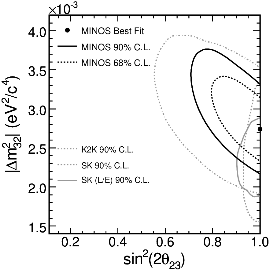
Another evidence of oscillations has been obtained from atmospheric neutrinos. The known discrepancy between the experimental observations and the predicted ratio of muon to electron neutrinos has become much stronger with the high precision and large statistics of Super-Kamiokande [86]. The atmospheric anomaly appears to originate in a reduction of the flux, and the data strongly favours the hypothesis. This result has been confirmed by K2K [87] and MINOS [88], observing the disappearance of accelerator ’s at distances of 250 and 735 Km, respectively. Super-Kamiokande has recently reported statistical evidence of appearance at the level [86]. The direct detection of the produced is the main goal of the ongoing CERN to Gran Sasso neutrino program.
Thus, we have now clear experimental evidence that neutrinos are massive particles and there is mixing in the lepton sector. Figures 35 and 35 show the present information on neutrino oscillations, from solar, atmospheric, accelerator and reactor neutrino data. A global analysis, combining the full set of data, leads to the following preferred ranges for the oscillation parameters [7]:
| (6.33) |
| (6.34) |
where are the mass squared differences between the neutrino mass eigenstates and the corresponding mixing angles in the standard three-flavour parametrization [7]. The ranges indicate 90% C.L. bounds. In the limit , solar and atmospheric neutrino oscillations decouple because . Thus, , and are constrained by solar data, while atmospheric experiments constrain , and . The angle is strongly constrained by the CHOOZ reactor experiment [89]. New planned reactor experiments, T2K and NOA are expected to achieve sensitivities around .

Non-zero neutrino masses constitute a clear indication of new physics beyond the SM. Right-handed neutrinos are an obvious possibility to incorporate Dirac neutrino masses. However, the fields would be singlets, without any SM interaction. If such objects do exist, it would seem natural to expect that they are able to communicate with the rest of the world through some still unknown dynamics. Moreover, the SM gauge symmetry would allow for a right-handed Majorana neutrino mass term,
| (6.35) |
where denotes the charge-conjugated field. The Majorana mass matrix could have an arbitrary size, because it is not related to the ordinary Higgs mechanism. Since both fields and absorb and create , the Majorana mass term mixes neutrinos and anti-neutrinos, violating lepton number by two units. Clearly, new physics is called for.
Adopting a more general effective field theory language, without any assumption about the existence of right-handed neutrinos or any other new particles, one can write the most general invariant Lagrangian, in terms of the known low-energy fields (left-handed neutrinos only). The SM is the unique answer with dimension four. The first contributions from new physics appear through dimension-5 operators, and have also a unique form which violates lepton number by two units [90]:
| (6.36) |
where denotes the -flavoured lepton doublet, and . Similar operators with quark fields are forbidden, due to their different hypercharges, while higher-dimension operators would be suppressed by higher powers of the new-physics scale . After SSB, , generates a Majorana mass term for the left-handed neutrinos, with44 4 This relation generalizes the well-known see-saw mechanism () [91, 92]. . Thus, Majorana neutrino masses should be expected on general symmetry grounds. Taking eV, as suggested by atmospheric neutrino data, one gets GeV, amazingly close to the expected scale of Gran Unification.
With non-zero neutrino masses, the leptonic charged-current interactions involve a flavour mixing matrix . The data on neutrino oscillations imply that all elements of are large, except for ; therefore the mixing among leptons appears to be very different from the one in the quark sector. The number of relevant phases characterizing the matrix depends on the Dirac or Majorana nature of neutrinos, because if one rotates a Majorana neutrino by a phase, this phase will appear in its mass term which will no longer be real. With only three Majorana (Dirac) neutrinos, the matrix involves six (four) independent parameters: three mixing angles and three (one) phases.
The smallness of neutrino masses implies a strong suppression of neutrinoless lepton-flavour-violating processes, which can be avoided in models with other sources of lepton-flavour violation, not related to . Table 5 shows the best published limits on lepton-flavour-violating decays. The B Factories are pushing the experimental limits on neutrinoless decays beyond the level, increasing in a drastic way the sensitivity to new physics scales. Future experiments could push further some limits to the level, allowing to explore interesting and totally unknown phenomena. Complementary information will be provided by the MEG experiment, which will search for events with a sensitivity of [93]. There are also ongoing projects at J-PARC aiming to study conversions in muonic atoms, at the level.
At present, we still ignore whether neutrinos are Dirac or Majorana fermions. Another important question to be addressed in the future concerns the possibility of leptonic CP violation and its relevance for explaining the baryon asymmetry of our Universe through leptogenesis.
7 Summary
The SM provides a beautiful theoretical framework which is able to accommodate all our present knowledge on electroweak and strong interactions. It is able to explain any single experimental fact and, in some cases, it has successfully passed very precise tests at the 0.1% to 1% level. In spite of this impressive phenomenological success, the SM leaves too many unanswered questions to be considered as a complete description of the fundamental forces. We do not understand yet why fermions are replicated in three (and only three) nearly identical copies. Why the pattern of masses and mixings is what it is? Are the masses the only difference among the three families? What is the origin of the SM flavour structure? Which dynamics is responsible for the observed violation?
In the gauge and scalar sectors, the SM Lagrangian contains only four parameters: , , and . We can trade them by , , and ; this has the advantage of using the three most precise experimental determinations to fix the interaction. In any case, one describes a lot of physics with only four inputs. In the fermionic flavour sector, however, the situation is very different. With , we have 13 additional free parameters in the minimal SM: 9 fermion masses, 3 quark mixing angles and 1 phase. Taking into account non-zero neutrino masses, we have three more mass parameters plus the leptonic mixings: three angles and one phase (three phases) for Dirac (or Majorana) neutrinos.
Clearly, this is not very satisfactory. The source of this proliferation of parameters is the set of unknown Yukawa couplings in Eq. (6). The origin of masses and mixings, together with the reason for the existing family replication, constitute at present the main open problem in electroweak physics. The problem of fermion mass generation is deeply related with the mechanism responsible for the electroweak SSB. Thus, the origin of these parameters lies in the most obscure part of the SM Lagrangian: the scalar sector. The dynamics of flavour appears to be ‘terra incognita’ which deserves a careful investigation.
The SM incorporates a mechanism to generate violation, through the single phase naturally occurring in the CKM matrix. Although the present laboratory experiments are well described, this mechanism is unable to explain the matter–antimatter asymmetry of our Universe. A fundamental explanation of the origin of -violating phenomena is still lacking.
The first hints of new physics beyond the SM have emerged recently, with convincing evidence of neutrino oscillations showing that and transitions do occur. The existence of lepton-flavour violation opens a very interesting window to unknown phenomena.
The Higgs particle is the main missing block of the SM framework. The successful tests of the SM quantum corrections with precision electroweak data confirm the assumed pattern of SSB, but do not prove the validity of the minimal Higgs mechanism embedded in the SM. The present experimental bounds (5.19) put the Higgs hunting within the reach of the new generation of detectors. The LHC should find out whether such scalar field indeed exists, either confirming the SM Higgs mechanism or discovering completely new phenomena.
Many interesting experimental signals are expected to be seen in the near future. New experiments will probe the SM to a much deeper level of sensitivity and will explore the frontier of its possible extensions. Large surprises may well be expected, probably establishing the existence of new physics beyond the SM and offering clues to the problems of mass generation, fermion mixing and family replication.
Acknowledgements
I want to thank the organizers for the charming atmosphere of this school and all the students for their many interesting questions and comments. This work has been supported by the EU MRTN-CT-2006-035482 (FLAVIAnet), MEC (Spain, FPA2004-00996) and Generalitat Valenciana (GVACOMP2007-156).
Appendix A Basic Inputs from Quantum Field Theory
1.1 Wave equations
The classical Hamiltonian of a non-relativistic free particle is given by . In quantum mechanics, energy and momentum correspond to operators acting on the particle wave function. The substitutions and lead then to the Schrödinger equation:
| (A.1) |
We can write the energy and momentum operators in a relativistic covariant way as , where we have adopted the usual natural units convention . The relation determines the Klein–Gordon equation for a relativistic free particle:
| (A.2) |
The Klein–Gordon equation is quadratic on the time derivative because relativity puts the space and time coordinates on an equal footing. Let us investigate whether an equation linear in derivatives could exist. Relativistic covariance and dimensional analysis restrict its possible form to
| (A.3) |
Since the r.h.s. is identically zero, we can fix the coefficient of the mass term to be ; this just determines the normalization of the four coefficients . Notice that should transform as a Lorentz four-vector. The solutions of Eq. (A.3) should also satisfy the Klein–Gordon relation of Eq. (A.2). Applying an appropriate differential operator to Eq. (A.3), one can easily obtain the wanted quadratic equation:
| (A.4) |
Terms linear in derivatives cancel identically, while the term with two derivatives reproduces the operator provided the coefficients satisfy the algebraic relation
| (A.5) |
which defines the so-called Dirac algebra. Eq. (A.3) is known as the Dirac equation.
Obviously the components of the four-vector cannot simply be numbers. The three Pauli matrices satisfy , which is very close to the relation (A.5). The lowest-dimensional solution to the Dirac algebra is obtained with matrices. An explicit representation is given by:
| (A.6) |
Thus, the wave function is a column vector with four components in the Dirac space. The presence of the Pauli matrices strongly suggests that it contains two components of spin . A proper physical analysis of its solutions shows that the Dirac equation describes simultaneously a fermion of spin and its own antiparticle [94].
It turns useful to define the following combinations of gamma matrices:
| (A.7) |
In the explicit representation (A.6),
| (A.8) |
The matrix is then related to the spin operator. Some important properties are:
| (A.9) |
Specially relevant for weak interactions are the chirality projectors ()
| (A.10) |
which allow to decompose the Dirac spinor in its left-handed and right-handed chirality parts:
| (A.11) |
In the massless limit, the chiralities correspond to the fermion helicities.
1.2 Lagrangian formalism
The Lagrangian formulation of a physical system provides a compact dynamical description and makes it easier to discuss the underlying symmetries. Like in classical mechanics, the dynamics is encoded in the action
| (A.12) |
The integral over the four space-time coordinates preserves relativistic invariance. The Lagrangian density is a Lorentz-invariant functional of the fields and their derivatives. The space integral would correspond to the usual non-relativistic Lagrangian.
The principle of stationary action requires the variation of the action to be zero under small fluctuations of the fields. Assuming that the variations are differentiable and vanish outside some bounded region of space-time (which allows an integration by parts), the condition determines the Euler–Lagrange equations of motion for the fields:
| (A.13) |
One can easily find appropriate Lagrangians to generate the Klein–Gordon and Dirac equations. They should be quadratic on the fields and Lorentz invariant, which determines their possible form up to irrelevant total derivatives. The Lagrangian
| (A.14) |
describes a complex scalar field without interactions. Both the field and its complex conjugate satisfy the Klein–Gordon equation; thus, describes a particle of mass without spin and its antiparticle. Particles which are their own antiparticles (i.e., with no internal charges) have only one degree of freedom and are described through a real scalar field. The appropriate Klein–Gordon Lagrangian is then
| (A.15) |
The Dirac equation can be derived from the Lagrangian density
| (A.16) |
The adjoint spinor closes the Dirac indices. The matrix is included to guarantee the proper behaviour under Lorentz transformations: is a Lorentz scalar, while transforms as a four-vector [94]. Therefore, is Lorentz invariant as it should.
Using the decomposition (A.11) of the Dirac field in its two chiral components, the fermionic Lagrangian adopts the form:
| (A.17) |
Thus, the two chiralities decouple if the fermion is massless.
1.3 Symmetries and conservation laws
Let us assume that the Lagrangian of a physical system is invariant under some set of continuous transformations
| (A.18) |
i.e., . One finds then that
| (A.19) |
If the fields satisfy the Euler–Lagrange equations of motion (A.13), the first term is identically zero; therefore the system has a conserved current:
| (A.20) |
This allows us to define a conserved charge
| (A.21) |
The condition guarantees that , i.e., that is a constant of motion.
This result, known as Noether’s theorem, can be easily extended to general transformations involving also the space-time coordinates. For every continuous symmetry transformation which leaves the Lagrangian invariant, there is a corresponding divergenceless Noether’s current and, therefore, a conserved charge. The selection rules observed in Nature, where there exist several conserved quantities (energy, momentum, angular momentum, electric charge, etc.), correspond to dynamical symmetries of the Lagrangian.
1.4 Classical electrodynamics
The well-known Maxwell equations,
| (A.22) | |||||
| (A.23) |
summarize a large amount of experimental and theoretical work and provide a unified description of the electric and magnetic forces. The first two equations in (A.22) are easily solved, writing the electromagnetic fields in terms of potentials:
| (A.24) |
It is very useful to rewrite these equations in a Lorentz covariant notation. The charge density and the electromagnetic current transform as a four-vector . The same is true for the potentials which combine into . The relations (A.24) between the potentials and the fields then take a very simple form, which defines the field strength tensor:
| (A.25) |
In terms of the tensor , the covariant form of the Maxwell equations turns out to be very transparent:
| (A.26) |
The electromagnetic dynamics is clearly a relativistic phenomenon, but Lorentz invariance was not very explicit in the original formulation of Eqs. (A.22) and (A.23). Once a covariant formulation is adopted, the equations become much simpler. The conservation of the electromagnetic current appears now as a natural compatibility condition:
| (A.27) |
In terms of potentials, is identically zero while adopts the form:
| (A.28) |
The same dynamics can be described by many different electromagnetic four-potentials, which give the same field strength tensor . Thus, the Maxwell equations are invariant under gauge transformations:
| (A.29) |
Taking the Lorentz gauge , Eq. (A.28) simplifies to
| (A.30) |
In the absence of an external current, i.e., with , the four components of satisfy then a Klein–Gordon equation with . The photon is therefore a massless particle.
The Lorentz condition still allows for a residual gauge invariance under transformations of the type (A.29), with the restriction . Thus, we can impose a second constraint on the electromagnetic field , without changing . Since contains four fields () and there are two arbitrary constraints, the number of physical degrees of freedom is just two. Therefore, the photon has two different physical polarizations
Appendix B SU(N) Algebra
is the group of unitary matrices, , with . Any matrix can be written in the form
| (B.1) |
with Hermitian, traceless matrices. Their commutation relations
| (B.2) |
define the algebra. The matrices generate the fundamental representation of the algebra. The basis of generators can be chosen so that the structure constants are real and totally antisymmetric.
For , are the usual Pauli matrices,
| (B.3) |
which satisfy the commutation relation
| (B.4) |
Other useful properties are: and .
For , the fundamental representation corresponds to the eight Gell-Mann matrices:
They satisfy the anticommutation relation
| (B.32) |
where denotes the -dimensional unit matrix and the constants are totally symmetric in the three indices.
For , the only non-zero (up to permutations) and constants are
| (B.33) | |||
The adjoint representation of the group is given by the matrices , which satisfy the commutation relations (B.2). The following equalities
| (B.34) | |||||
define the invariants , and . Other useful properties are:
| (B.35) |
Appendix C Anomalies

Our theoretical framework is based on the local gauge symmetry. However, so far we have only discussed the symmetries of the classical Lagrangian. It happens sometimes that a symmetry of gets broken by quantum effects, i.e., it is not a symmetry of the quantized theory; one says then that there is an ‘anomaly’. Anomalies appear in those symmetries involving both axial () and vector () currents, and reflect the impossibility of regularizing the quantum theory (the divergent loops) in a way which preserves the chiral (left/right) symmetries.
A priori there is nothing wrong with having an anomaly. In fact, sometimes they are even welcome. A good example is provided by the decay . There is a chiral symmetry of the QCD Lagrangian which forbids this transition; the should then be a stable particle, in contradiction with the experimental evidence. Fortunately, there is an anomaly generated by a triangular quark loop (Fig. 36) which couples the axial current to two electromagnetic currents and breaks the conservation of the axial current at the quantum level:
| (C.1) |
Since the couples to , , the decay does finally occur, with a predicted rate
| (C.2) |
where denotes the number of quark colours and the so-called pion decay constant, MeV, is known from the decay rate (assuming isospin symmetry). The agreement with the measured value, eV [7], is excellent.
Anomalies are, however, very dangerous in the case of local gauge symmetries, because they destroy the renormalizability of the Quantum Field Theory. Since the model is chiral (i.e., it distinguishes left from right), anomalies are clearly present. The gauge bosons couple to vector and axial-vector currents; we can then draw triangular diagrams with three arbitrary gauge bosons (, , ) in the external legs. Any such diagram involving one axial and two vector currents generates a breaking of the gauge symmetry. Thus, our nice model looks meaningless at the quantum level.
We have still one way out. What matters is not the value of a single Feynman diagram, but the sum of all possible contributions. The anomaly generated by the sum of all triangular diagrams connecting the three gauge bosons , and is proportional to
| (C.3) |
where the traces sum over all possible left- and right-handed fermions, respectively, running along the internal lines of the triangle. The matrices are the generators associated with the corresponding gauge bosons; in our case, .
In order to preserve the gauge symmetry, one needs a cancellation of all anomalous contributions, i.e., . Since , we have an automatic cancellation in two combinations of generators: and . However, the other two combinations, and turn out to be proportional to , i.e., to the sum of fermion electric charges:
| (C.4) |
Equation (C.4) conveys a very important message: the gauge symmetry of the model does not have any quantum anomaly, provided that . Fortunately, this is precisely the right number of colours to understand strong interactions. Thus, at the quantum level, the electroweak model seems to know something about QCD. The complete SM gauge theory based on the group is free of anomalies and, therefore, renormalizable. The anomaly cancellation involves one complete generation of leptons and quarks: . The SM would not make any sense with only leptons or quarks.
References
- [1] Updated version of the lectures given at the 2004 European School of High-Energy Physics (San Feliu de Guixols, Spain): A. Pich, The Standard Model of Electroweak Interactions, Report CERN-2006-003, ed. R. Fleischer, p. 1 [arXiv:hep-ph/0502010].
- [2] S.L. Glashow, Nucl. Phys. 22 (1961) 579.
- [3] S. Weinberg, Phys. Rev. Lett. 19 (1967) 1264.
- [4] A. Salam, in Elementary Particle Theory, ed. N. Svartholm (Almquist and Wiksells, Stockholm, 1969), p. 367.
- [5] S.L. Glashow, J. Iliopoulos and L. Maiani, Phys. Rev. D2 (1970) 1285.
- [6] A. Pich, Aspects of Quantum Chromodynamics, arXiv:hep-ph/0001118.
- [7] W.-M. Yao et al., Review of Particle Physics, J. Phys. G33 (2006) 1.
- [8] B. Odom et al., Phys. Rev. Lett. 97 (2006) 030801.
- [9] Muon Collaboration, Phys. Rev. D73 (2006) 072003.
- [10] M. Davier and W.J. Marciano, Annu. Rev. Nucl. Part. Sci. 54 (2004) 115.
- [11] J.P. Miller, E. de Rafael and B.L. Roberts, arXiv:hep-ph/0703049.
- [12] T. Kinoshita and M. Nio, Phys. Rev. D73 (2006) 013003, 053007; D70 (2004) 113001; Phys. Rev. Lett. 90 (2003) 021803.
- [13] T. Aoyama et al., Nucl. Phys. B740 (2006) 138.
- [14] A.L. Kataev, Phys. Rev. D74 (2006) 073011.
- [15] G. Gabrielse et al., Phys. Rev. Lett. 97 (2006) 030802.
- [16] M. Davier et al., Eur. Phys. J. C27 (2003) 497; C31 (2003) 503.
- [17] M. Davier, arXiv:hep-ph/0701163.
- [18] A. Pich, arXiv:hep-ph/0702074.
- [19] J. Bijnens and J. Prades, Mod. Phys. Lett. A22 (2007) 767.
- [20] H. Fritzsch and M. Gell-Mann, Proc. XVI International Conference on High Energy Physics, eds. J.D. Jackson and A. Roberts (Fermilab, 1972), Vol. 2, p. 135.
- [21] H. Fritzsch, M. Gell-Mann and H. Leutwyler, Phys. Lett. B47 (365) 1973.
- [22] ALEPH Collaboration, http://aleph.web.cern.ch/aleph/dali/Z0_examples.html.
- [23] A. Pich, arXiv:hep-ph/9412274.
- [24] Tevatron Electroweak Working Group, arXiv:hep-ex/0703034.
- [25] J. Goldstone, Nuov. Cim. 19 (1961) 154.
- [26] P.W. Higgs, Phys. Rev. 145 (1966) 1156.
- [27] T.W.B. Kibble, Phys. Rev. 155 (1967) 1554.
- [28] G. ’t Hooft, Nucl. Phys. B33 (1971) 173.
- [29] The LEP Collaborations ALEPH, DELPHI, L3 and OPAL and the LEP Electroweak Working Group, arXiv:hep-ex/0612034; http://www.cern.ch/LEPEWWG/.
- [30] The ALEPH, DELPHI, L3, OPAL and SLD Collaborations, the LEP Electroweak Working Group and the SLD Electroweak and Heavy Flavour Groups, Phys. Rept. 427 (2006) 257.
- [31] MuLan Collaboration, arXiv:0704.1981 [hep-ex].
- [32] W.J. Marciano and A. Sirlin, Phys. Rev. Lett. 61 (1988) 1815.
- [33] T. van Ritbergen and R.G. Stuart, Phys. Rev. Lett. 82 (1999) 488.
- [34] M. Moulson, arXiv:hep-ex/0703013; FLAVIAnet Kaon Working Group, http://ific.uv.es/flavianet/.
- [35] S. Bethke, Prog. Part. Nucl. Phys. 58 (2007) 351.
- [36] D.J. Gross and F. Wilczek, Phys. Rev. Lett. 30 (1973) 1343.
- [37] H.D. Politzer, Phys. Rev. Lett. 30 (1973) 1346.
- [38] T. Appelquist and J. Carazzone, Phys. Rev. D11 (1975) 2856.
- [39] M. Veltman, Nucl. Phys. B123 (1977) 89.
- [40] J. Bernabéu, A. Pich and A. Santamaría, Phys. Lett. B200 (1988) 569; Nucl. Phys. B363 (1991) 326.
- [41] A.A. Akhundov, D. Yu. Bardin and T. Riemann, Nucl. Phys. B276 (1986) 1.
- [42] W. Beenakker and W. Hollik, Z. Phys. C40 (1988) 141.
- [43] B.W. Lynn and R.G. Stuart, Phys. Lett. B252 (1990) 676.
- [44] D. Denegri, http://cmsinfo.cern.ch/Welcome.html/CMSdocuments/CMSplots/CMSplots.html.
- [45] N. Cabibbo, Phys. Rev. Lett. 10 (1963) 531.
- [46] M. Kobayashi and T. Maskawa, Prog. Theor. Phys. 42 (1973) 652.
- [47] SINDRUM Collaboration, Nucl. Phys. B299 (1988) 1.
- [48] MEGA/LAMPF Collaboration, Phys. Rev. Lett. 83 (1999) 1521.
- [49] BELLE Collaboration, arXiv:0705.0650 [hep-ex]; Phys. Lett. B640 (2006) 138; 639 (2006) 159; 632 (2006) 51; 622 (2005) 218; 589 (2004) 103; Phys. Rev. Lett. 93 (2004) 081803; 92 (2004) 171802.
- [50] BABAR Collaboration, Phys. Rev. Lett. 98 (2007) 061803; 96 (2006) 041801; 95 (2005) 191801, 041802; 92 (2004) 121801.
- [51] A. Pich, arXiv:hep-ph/9601202.
- [52] E. Gámiz, M. Jamin, A. Pich, J. Prades and F. Schwab, Phys. Rev. Lett. 94 (2005) 011803; JHEP 0301 (2003) 060; arXiv:hep-ph/0612154.
- [53] W. J. Marciano, Phys. Rev. Lett. 93 (2004) 231803.
- [54] M. Jamin, J.A. Oller and A. Pich, Phys. Rev. D74 (2006) 074009.
- [55] MILC Collaboration, arXiv:hep-lat/0611024.
- [56] N. Isgur and M. Wise, Phys. Lett. B232 (1989) 113; B237 (1990) 527.
- [57] B. Grinstein, Nucl. Phys. B339 (1990) 253.
- [58] E. Eichten and B. Hill, Phys. Lett. B234 (1990) 511.
- [59] H. Georgi, Phys. Lett. B240 (1990) 447.
- [60] M. Neubert, Phys. Lett. B264 (1991) 455.
- [61] M. Luke, Phys. Lett. B252 (1990) 447.
- [62] D. Počanić et al., Phys. Rev. Lett. 93 (2004) 181803.
- [63] J. Portolés, arXiv:hep-ph/0703093.
- [64] V. Mateu and A. Pich, JHEP 0510 (2005) 041.
- [65] R. Flores-Mendieta, Phys. Rev. D70 (2004) 114036.
- [66] N. Cabibbo, E.C. Swallow and R. Winston, Ann. Rev. Nucl. Part. Sci. 53 (2003) 39; Phys. Rev. Lett. 92 (2004) 251803.
- [67] Heavy Flavour Averaging Group, arXiv:0704.3575 [hep-ex].
- [68] CDF Collaboration, Phys. Rev. Lett. 95 (2005) 102002.
- [69] D0 Collaboration, Phys. Lett. B639 (2006) 616.
- [70] D0 Collaboration, Phys. Rev. Lett. 98 (2007) 181802.
- [71] L. Wolfenstein, Phys. Rev. Lett. 51 (1983) 1945.
- [72] A.J. Buras, M.E. Lautenbacher and G. Ostermaier, Phys. Rev. D50 (1994) 3433.
- [73] C. Jarlskog, Phys. Rev. Lett. 55 (1985) 1039; Z. Phys. C29 (1985) 491.
- [74] CDF Collaboration, Phys. Rev. Lett. 97 (2006) 242003.
- [75] A.B. Carter and A.I. Sanda, Phys. Rev. Lett. 45 (1980) 952; Phys. Rev. D23 (1981) 1567.
- [76] I.I. Bigi and A.I. Sanda, Nucl. Phys. B193 (1981) 85.
- [77] CKMfitter Group, Eur. Phys. J. C41 (2005) 1; http://ckmfitter.in2p3.fr/.
- [78] I.I. Bigi, arXiv:hep-ph/0701273.
- [79] UTfit Collaboration, JHEP 0610 (2006) 081; http://utfit.roma1.infn.it/.
- [80] A.J. Buras, arXiv:hep-ph/0505175.
- [81] R. Davis et al., Phys. Rev. Lett. 20 (1968) 1205.
- [82] J. Bahcall and M.H. Pinsonneault, Phys. Rev. Lett. 92 (2004) 121301.
- [83] SNO Collaboration, Phys. Rev. Lett. 89 (2002) 011301, 011302; 92 (2004) 181301; Phys. Rev. C72 (2005) 055502; arXiv:nucl-ex/0610020.
- [84] Super-Kamiokande Collaboration, Phys. Rev. Lett. 86 (2001) 5656; Phys. Lett. B539 (2002) 179; Phys. Rev. D69 (2004) 011104; 68 (2003) 092002.
- [85] KamLAND Collaboration, Phys. Rev. Lett. 90 (2003) 021802; 92 (2004) 071301; 94 (2005) 081801.
- [86] Super-Kamiokande Collaboration, Phys. Rev. Lett. 81 (1998) 1562; 82 (1999) 2644, 5194; 85 (2000) 3999; 93 (2004) 101801; 97 (2006) 171801; Phys. Rev. D71 (2005) 112005.
- [87] K2K Collaboration, Phys. Rev. D74 (2006) 072003; Phys. Rev. Lett. 90 (2003) 041801; 94 (2005) 081802.
- [88] MINOS Collaboration, Phys. Rev. Lett. 97 (2006) 191801.
- [89] CHOOZ Collaboration, Phys. Lett. B466 (1999) 415.
- [90] S. Weinberg, Phys. Rev. Lett. 43 (1979) 1566.
- [91] M. Gell-Mann, P. Ramond and R. Slansky, Complex Spinors and Unified Theories, in Supergravity, eds. P. van Nieuwenhuizen and D.Z. Freedman (North Holland, Stony Brook 1979) p. 315.
- [92] T. Yanagida, in Proc. Workshop on Unified Theory and Baryon Number in the Universe, eds. O. Sawada and A. Sugamoto (KEK, 1979) p. 95.
- [93] MEG Collaboration, Nucl. Phys. B (Proc. Suppl.) 162 (2006) 279.
- [94] J.D. Bjorken and S.D. Drell, Relativistic Quantum Mechanics, McGraw-Hill (New York, 1964).