Maximally Entangled Mixed-State Generation via Local Operations

Entanglement is perhaps the most puzzling feature of quantum mechanics and in the last two decades it became the key resource in quantum information processing Nielsen and Chuang 2002. Entangled qubits prepared in pure, maximally entangled states are required by many quantum-information processes. However, in a mundane world, a pure maximally entangled state is an idealization as, e.g., a plane wave in classical optics. In fact, interaction of qubits with the environment leads to decoherence that may cause a pure entangled state to become less pure (mixed) and less entangled. Thus, any realistic quantum-communication/computation protocol must cope with entangled mixed states and it is desirable to attain the maximum amount of entanglement for a given degree of mixedness. States that fulfill this condition are called maximally entangled mixed states (MEMS) and, recently, they have been the subject of several papers (see, e.g., Peters et al. 2004; Barbieri et al. 2004 and references therein). In this Article we propose a new method to create MEMS from a pair of photons initially prepared in the singlet polarization state.

Kwiat and coworkers Peters et al. 2004 were the first to achieve MEMS using photon pairs from spontaneous parametric down conversion (SPDC). They induced decoherence in SPDC pairs initially prepared in a pure entangled state by coupling polarization and time degrees of freedom of the photons. At the same time, a somewhat different scheme was used by De Martini and coworkers Barbieri et al. 2004 who instead used the spatial degrees of freedom of SPDC photons to induce decoherence. However, both the Kwiat and the De Martini method require operations on both photons of the SPDC pair. On the contrary, our technique has the advantage to require only local operations upon one of the two photons.

This Article is structured as follows: In the first part of Sec. II we show the relation existing between a one-qubit quantum map and a classical-optics setup on the laboratory bench. In the second part of Sec. II, we exploit this knowledge to design a simple linear-optical set-up to generate MEMS from a pair of photons via local operations and postselection. Then, in Sec. III we provide an experimental demonstration of our method, using entangled photons from parametric down-conversion. Finally, we draw our conclusions in Sec. IV.

We begin by giving a brief description of the connection between classical polarization optics and quantum mechanics of qubits, as recently put forward by several authors Brunner et al. 2003; Aiello et al. 2006. Most textbooks on classical optics introduce the concept of polarized and unpolarized light with the help of the Jones and Stokes-Mueller calculi, respectively Damask 2005. In these calculi, the description of classical polarization of light is formally identical to the quantum description of pure and mixed states of two-level systems, respectively Iso. Mathematically speaking, there is an isomorphism between the quantum density matrix $\rho$ describing a qubit and the classical coherency matrix $J$ Born and Wolf 1999 describing polarization of a beam of light: $\rho\sim J/\mathrm{Tr}J$. $J$ is an Hermitean, positive semidefinite $2\times 2$ matrix, as is $\rho$. A classical linear optical process (as, e.g., the passage of a beam of light through an optical device), can be described by a $4\times 4$ complex-valued matrix $\mathcal{M}$ such that $(J_{\mathrm{out}})_{ij}=\mathcal{M}_{ij,kl}(J_{\mathrm{in}})_{kl}$, where, from now on, we adopt the convention that summation over repeated Latin indices is understood. Moreover, we assume that all Latin indices $i,j,k,l,m,n,\ldots$ take the values $0$ and $1$, while Greek indices $\alpha,\beta,\dots$ take the values $0,1,2,3$. In polarization optics one usually deals with the real-valued Mueller matrix $M$ which is connected to $\mathcal{M}$ via a unitary transformation $\Lambda:M=\Lambda^{\dagger}\mathcal{M}\Lambda$ Aie a. The matrix $M$ is often written as Lu and Chipman 1996

where $(\mathbf{p},\mathbf{d})\in\mathbb{R}^{3}$, are known as the polarizance vector and the diattenuation vector (superscript $T$ indicates transposition), respectively. Note that $\mathbf{d}$ is nonzero only for dichroic media, namely media that induce polarization-dependent losses (PDL) Damask 2005. $W$ is a $3\times 3$ real-valued matrix. It should be noticed that if we choose $m_{00}=1$ (this can be always done since it amounts to a trivial polarization-independent renormalization), the Mueller matrix of a non-dichroic optical element ($\mathbf{d}=\mathbf{0}$), is formally identical to a non-unital, trace-preserving, one-qubit quantum map (also called channel) Ruskai et al. 2002. If also $\mathbf{p}=\mathbf{0}$ (pure depolarizers and pure retarders Damask 2005), then $M$ becomes identical to a unital, one-qubit channel Nielsen and Chuang 2002. It is not difficult to show that any linear optical device that can be represented by $\mathcal{M}$ (or $M$), can also be described by a set of at most four distinct optical elements in parallel as $\mathcal{M}=\sum_{\alpha}\lambda_{\alpha}T_{\alpha}\otimes T_{\alpha}^{*}$, where the four $2\times 2$ Jones matrices $T_{\alpha}$, represent four different non-depolarizing optical elements and $\lambda_{\alpha}\geq 0$ Anderson and Barakat 1994; Aie a . From the results above it readily follows that the most general operation that a linear optical element can perform upon a beam of light can be written as $J_{\mathrm{in}}\rightarrow J_{\mathrm{out}}=\sum_{\alpha}\lambda_{\alpha}T_{\alpha}J_{\mathrm{in}}T_{\alpha}^{\dagger}$. Since $\lambda_{\alpha}\geq 0$, the previous equation is formally identical to the Kraus form Nielsen and Chuang 2002 of a completely positive one-qubit quantum map $\mathcal{E}$. Therefore, if a single photon encoding a polarization qubit passes through an optical device classically described by the Mueller matrix $\mathcal{M}=\sum_{\alpha}\lambda_{\alpha}T_{\alpha}\otimes T_{\alpha}^{*}$, its initial state $\rho_{\mathrm{in}}$ will be transformed according to $\rho_{\mathrm{in}}\rightarrow\rho_{\mathrm{out}}\propto\sum_{\alpha}\lambda_{\alpha}T_{\alpha}\rho_{\mathrm{in}}T_{\alpha}^{\dagger}$.

Now that we have learned how to associate a quantum map to a set of at most four optical elements, we can apply this knowledge to design a simple optical scheme suitable for MEMS production. Suppose to have two qubits (encoded in the polarization degrees of freedom of two SPDC photons, say $A$ and $B$), initially prepared in the state $\rho:\rho=\rho_{ij,kl}|ij\rangle\langle kl|\doteq\rho_{ik,jl}^{R}|i\rangle\langle k|\otimes|j\rangle\langle l|$. Superscript $R$ indicates reshuffling Zic of the indices: $\rho_{ik,jl}^{R}\equiv\rho_{ij,kl}$. Following Ziman and Bužek Ziman and Bužek 2005 we assume that $\rho$ is transformed under the action of the most general local (that is, acting upon a single qubit) linear map $\mathcal{E}\otimes\mathcal{I}$ into the state

By writing explicitly Eq. (2) in the two-qubit basis $\{|ij\rangle\equiv|i\rangle\otimes|j\rangle\}$, it is straightforward to obtain $(\rho_{\mathcal{E}})_{ij,kl}\propto\sum_{\alpha}\lambda_{\alpha}\rho^{R}_{mn,jl}(T_{\alpha})_{im}(T^{*}_{\alpha})_{kn}$. Then, from the definition of $\mathcal{M}$ it easily follows that $(\rho_{\mathcal{E}})_{ij,kl}\propto(\mathcal{M}\rho^{R})_{ik,jl}$. By reshuffling $\rho_{\mathcal{E}}$, this last result can be written in matrix form as $\rho_{\mathcal{E}}^{R}\propto\mathcal{M}\rho^{R}$ which displays the very simple relation existing between the classical Mueller matrix $\mathcal{M}$ and the quantum state $\rho_{\mathcal{E}}$. Via a direct calculation, it is possible to show that if $\rho$ represents two qubits in the singlet state $\rho_{s}=\frac{1}{4}(I\otimes I-\sigma_{x}\otimes\sigma_{x}-\sigma_{y}\otimes\sigma_{y}-\sigma_{z}\otimes\sigma_{z})$ Pau, then the proportionality symbol in the last equation above can be substituted with the equality symbol: $\rho_{\mathcal{E}}^{R}=\mathcal{M}\rho^{R}_{s}$. Note that this pleasant property is true only for the singlet state. However, if the initial state $\rho$ is different from the singlet one, then $\mathcal{M}$ must be simply renormalized by imposing $\mathrm{Tr}(\mathcal{M}\rho^{R})=1$ .

Now, suppose that we have an experimental setup producing pairs of SPDC photons in the singlet state $\rho_{s}$, and we want to transform $\rho_{s}$ into the target state $\rho_{\mathcal{T}}$ via a local map $\mathcal{T}\otimes\mathcal{I}:\,\rho_{s}\rightarrow\rho_{\mathcal{T}}=(\mathcal{M}_{\mathcal{T}}\rho_{s}^{R})^{R}$. All we have to do is first to invert the latter equation to obtain

and then to decompose $\mathcal{M}_{\mathcal{T}}$ as $\mathcal{M}_{\mathcal{T}}=\sum_{\alpha}\lambda_{\alpha}T_{\alpha}\otimes T_{\alpha}^{*}$. Thus, we get the (at most four) Jones matrices $T_{\alpha}$ representing the optical elements necessary to implement the desired transformation. This is the main theoretical result of this Article. Our technique is very straightforward and we shall demonstrate its feasibility later, by applying it to design an optical setup devoted to MEMS generation. However, at this moment, some caveats are in order. To make $\mathcal{M}_{\mathcal{T}}$ a physically realizable Mueller matrix, its associated matrix $H_{\mathcal{T}}$ should be positive semidefinite Not a. If this is not the case, then the transformation $\rho\rightarrow\rho_{\mathcal{T}}$ cannot be implemented via local operations. For example, it is easy to see that if the initial state is a Werner state $\rho_{W}=p\rho_{s}+\frac{1-p}{4}I,\;(0\leq p\leq 1)$ and the target state is the singlet $\rho_{\mathcal{T}}=\rho_{s}$, then such operation (known as concentration Thew and Munro 2001) cannot be physically implemented by a local setup since $H_{\mathcal{T}}$ has three degenerate negative eigenvalues. Another caveat comes from the no-signalling constraint. Since $\mathcal{M}_{\mathcal{T}}$ describes a local device operating only upon photon $A$, a second observer watching at photon $B$ cannot distinguish the initial state $\rho_{s}$ from the transformed state $\rho_{\mathcal{T}}$, that is: $\rho^{B}=\mathrm{Tr}_{A}(\rho_{s})=\mathrm{Tr}_{A}(\rho_{\mathcal{T}})$. This condition requires the one-qubit map $\mathcal{T}$ to be trace-preserving: $\sum_{\alpha}\lambda_{\alpha}T_{\alpha}^{\dagger}T_{\alpha}=I$. From Eq. (1), a straightforward calculation shows that such condition cannot be fulfilled if $\mathbf{d}\neq\mathbf{0}$, that is if the device implementing $\mathcal{T}$ contains dichroic (or PDL) elements.

PDL is important in many commonly used optical devices as polarizers, circulators, isolators, etc., Damask 2005. Within the framework of quantum information theory, all these physical devices may be represented by “unphysical” one-qubit maps $\mathcal{T}$ that violate the no-signalling condition. This apparent paradox disappears if one allows causal classical communications between observers who actually measure and reconstruct the target state $\rho_{\mathcal{T}}$ generated by the “unphysical” local map $\mathcal{T}\otimes\mathcal{I}$ Aie b. In fact, in coincidence measurements (required to reconstruct $\rho_{\mathcal{T}}$), classical (as opposed to quantum) signalling between the two observers is necessary to allow them to compare their own experimental results and select from the raw data the coincidence counts. In other words, a coincidence measurement post-selects only those photons that have not been absorbed by the PDL element Brunner et al. 2003.

With these caveats in mind, we come to the experimental validation of our method. We choose to generate MEMS I states Not b, represented by the density matrix $\rho_{\mathrm{I}}=p|\phi_{+}\rangle\langle\phi_{+}|+(1-p)|01\rangle\langle 01|$, where $|\phi_{+}\rangle=(|00\rangle+|11\rangle)/\sqrt{2}$ and $(2/3\leq p\leq 1)$. By varying the parameter $p$, the entanglement and mixedness of the state $\rho_{\mathrm{I}}$ change. Here, we use the linear entropy $S_{L}$ Bose and Vedral 2001 and the tangle $T$, namely, the concurrence squared Wootters 1998, to quantify the degree of mixedness and of entanglement, respectively. They are defined as $S_{L}(\rho)=\frac{4}{3}[1-\mathrm{Tr}(\rho^{2})]$, and $T(\rho)=[\max\{0,\sqrt{\lambda_{0}}-\sqrt{\lambda_{1}}-\sqrt{\lambda_{2}}-\sqrt{\lambda_{3}}\}]^{2}$, where $\lambda_{0}\geq\lambda_{1}\geq\lambda_{2}\geq\lambda_{3}\geq 0$ are the eigenvalues of $\rho(\sigma_{y}\otimes\sigma_{y})\rho^{*}(\sigma_{y}\otimes\sigma_{y})$. After applying Eq. (3) with $\rho_{\mathcal{T}}=\rho_{\mathrm{I}}$, a straightforward calculation shows that there are only two non-zero terms in the decomposition of $\mathcal{M}_{\mathcal{T}}$, namely $\{\lambda_{0}=2(1-p),\lambda_{1}=p\}$, $\{T_{0}=\left(\begin{array}[]{cc}1&0\\ 0&0\\ \end{array}\right),T_{1}=\left(\begin{array}[]{cc}0&-1\\ 1&0\\ \end{array}\right)\}$. In physical terms, $T_{0}$ is a polarizer and $T_{1}$ is a $90^{\circ}$ polarization rotator. The two eigenvalues $\{\lambda_{0},\lambda_{1}\}$ give the relative intensity in the two arms of the device and are physically realized by intensity attenuators.

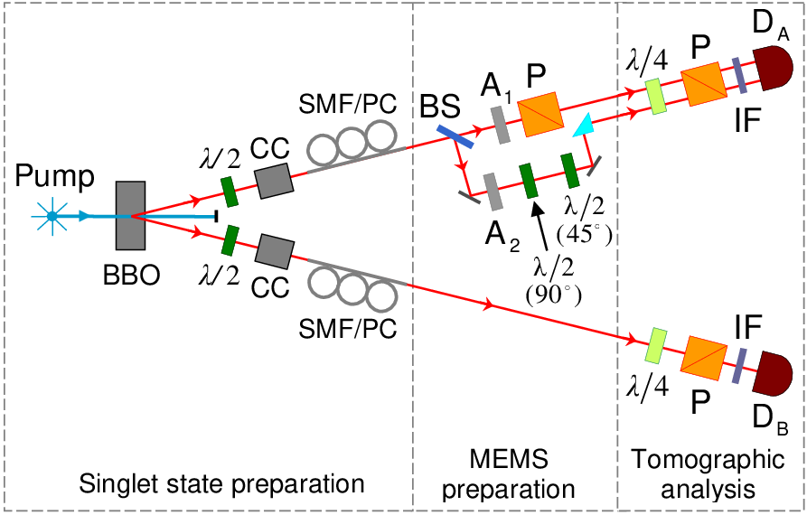
Our experimental set-up is shown in Fig.1. Its first part (Singlet state preparation) comprises a Krypton-ion laser at 413.1 nm that pumps a 1-mm thick $\beta-\mathrm{Ba}\mathrm{B}_{2}\mathrm{O}_{4}$ (BBO) crystal, where polarization-entangled photon pairs at wavelength 826.2 nm are created by SPDC in degenerate type II phase-matching configuration Kwiat et al. 1995. Single-mode fibers (SMF) are used as spatial filters to assure that the initial two-photon state is in a single transverse mode. Spurious birefringence along the fibers is compensated by suitably oriented polarization controllers (PC) Puentes et al. 2006. In addition, total retardation introduced by the fibers and walk-off effects at the BBO crystal are compensated by compensating crystals (CC: 0.5-mm thick BBO crystals) and half-wave plates ($\lambda/2$) in both photonic paths. In this way the initial two-photon state is prepared in the polarization singlet state $|\psi_{s}\rangle=(|HV\rangle-|VH\rangle)/\sqrt{2}$, where $H(=0)$ and $V(=1)$ are labels for horizontal and vertical polarizations of the two photons, respectively.

In the second part of the experimental set-up (MEMS preparation) the two-term decomposition of $\mathcal{M}_{\mathcal{T}}$ is physically realized by a two-path optical device. A photon enters such a device through a $50/50$ beam splitter (BS) and can be either transmitted to path $1$ or reflected to path $2$. The two paths defines two independent spatial modes of the field. In path $1$ a neutral-density filter ($\mathrm{\textsf{A}}_{1}$) is followed by a linear polarizer (P) oriented horizontally (with respect to the BBO crystal basis). When the photon goes in this path, the initial singlet is reduced to $|HV\rangle$ with probability proportional to the attenuation ratio $a_{1}$ of $\mathrm{\textsf{A}}_{1}$ ($a=P_{\mathrm{out}}/P_{\mathrm{in}}$). In path $2$ a second neutral-density filter ($\mathrm{\textsf{A}}_{2}$) is followed by two half wave-plates ($\lambda/{2}$) in cascade relatively oriented at $45^{\circ}$: they work as a $90^{\circ}$ polarization rotator. When the photon goes in path $2$, the singlet undergoes a local rotation with probability proportional to the attenuation ratio $a_{2}$ of $\mathrm{\textsf{A}}_{2}$.

The third and last part of the experimental set-up (Tomographic analysis), consists of two tomographic analyzers (one per photon), each made of a quarter-wave plate ($\lambda/4$) followed by a linear polarizer (P). Such analyzers permit a tomographically complete reconstruction, via a maximum-likelihood technique James et al. 2001, of the two-photon state. Additionally, interference filters (IF) in front of each detector ($\Delta\lambda=5$ nm) provide for bandwidth selection. It should be noticed that detector $\mathrm{\textsf{D}}_{\mathrm{\textsf{A}}}$ does not distinguish which path (either $1$ or $2$) a photon comes from, thus photon $A$ is detected in a mode-insensitive way: This is the simple mechanism we use to induce decoherence. In the actual setup, a lens (not shown in Fig. 1) placed in front of detector $\mathrm{\textsf{D}}_{\mathrm{\textsf{A}}}$ focusses both paths $1$ and $2$ upon the sensitive area of the detector which becomes thus unable to distinguish between photons coming from either path $1$ or $2$ (“mode-insensitive detection”).

Experimental results are shown in Fig. 2 together with theoretical predictions in the linear entropy-tangle plane. The agreement between theoretical predictions and measured data is very good. The experimentally prepared initial singlet state $\rho_{s}^{\mathrm{exp}}$ has a fidelity Jozsa 1994 $F(\rho_{s},\rho_{s}^{\mathrm{exp}})=\left|\mathrm{Tr}(\sqrt{\sqrt{\rho_{s}}\rho_{s}^{\mathrm{exp}}\sqrt{\rho_{s}}})\right|^{2}\sim 97\%$ with the theoretical singlet state $\rho_{s}$. The continuous curve is calculated from the matrix $\rho_{c}:\rho_{c}=\mathcal{M}_{\mathcal{T}}\rho_{s}^{\mathrm{exp}}$, and varying $p$. It represents our theoretical prediction for the given initially prepared state $\rho_{s}^{\mathrm{exp}}$. If it were possible to achieve exactly $\rho_{s}^{\mathrm{exp}}=\rho_{s}$, then such curve would coincide with the MEMS curve above the horizontal (dotted) line $T=4/9$. Experimental points with $T\geq 4/9$ ($\rho_{\mathrm{I}}^{\mathrm{exp}}$) are obtained by varying the neutral-density filters $\mathrm{\textsf{A}}_{1},\mathrm{\textsf{A}}_{2}$ in such a way that $a_{2}\geq a_{1}$; while points with $T<4/9$ are achieved for $a_{2}<a_{1}$. Note that the latter points do not represent MEMSs, but different mixed entangled states whose density matrix is still given by $\rho_{\mathrm{I}}$ but with the parameter $p$ now varying as $0\leq p\leq 2/3$. The average fidelity between the measured states $\rho_{\mathrm{I}}^{\mathrm{exp}}$ an the “target” states $\rho_{\star}$, is given by $\overline{F(\rho_{\star},\rho_{\mathrm{I}}^{\mathrm{exp}})}\sim 80\%$. The main reason for its deviation from $\lesssim 100\%$, is due to spurious, uncontrolled birefringence in the BS and the prism composing the set-up. To verify this, first we calculated the fidelity between the states $\rho_{c}(p)$ (obtained by applying the theoretically determined map $\mathcal{T}\otimes\mathcal{I}$ to the experimentally prepared initial singlet state $\rho_{s}^{\mathrm{exp}}$), with the theoretical MEMS $\rho_{\mathrm{I}}(p)$. We have found $F[\rho_{\mathrm{I}}(p),\rho_{c}(p)]\geq 97\%$ for all $2/3\leq p\leq 1$; thus the value of $\overline{F}\sim 80\%$ cannot be ascribed to the imperfect initial singlet preparation. Second, we explicitly measured the Mueller matrices for both the BS and the prism (matrices that would be equal to the identity for ideal non-birefringent elements) and we actually found spurious birefringence. From such measured matrices it was possible to determine the unwanted local unitary operation induced by these optical elements Aiello07. It is important to notice that such operation does not change the position of our experimental points in the linear entropy-tangle plane. Now, if one applies this unitary operation to our raw data and calculates once again the average fidelity, the result would be $\overline{F}\sim 91\%$. However, since this “compensation” of the spurious birefringence is performed upon the measured data and not directly on the physical setup, we felt that it was more fair to present the uncorrected data.

In conclusion, we have theoretically proposed and experimentally tested a new, simple method to create MEMS I states of photons. This method can be easily generalized to generate MEMS II states, as well. However, this task would require a slightly different experimental setup with a three-path linear optical device acting only upon photon $A$ Aiello07. In particular, we have shown that it is possible to create a MEMS from a SPDC photon pair, by acting on just a single photon of the pair. This task could appear, at first sight, impossible since it was recently demonstrated Ziman and Bužek 2005 that even the most general local operation cannot generate MEMS because this would violate relativistic causality. However, as we discussed in the text, our results do not contradict Ref. Ziman and Bužek 2005 since we obtained them via postselection operated by coincidence measurements. The latter are possible only when causal classical communication between detectors is permitted. Still, the connection between relativistic causality, dichroic (or, PDL) devices and postselection, is far from being trivial. For example, suppose that a two-photon state is produced by an optical setup containing local PDL elements, and that we tomographically reconstruct it after coincidence measurements. Such a reconstructed state will correctly describe the result of any other measurement involving coincidence measurements (as, e.g., Bell measurements), but it will fail when describing the result of any single-photon measurement. We stress that this limitation is not inherent to our scheme, but it is shared by all optical set-ups containing PDL elements.