New smooth hybrid inflationPreprint: UT–STPD–2/07

Setting $\gamma=0$, the F-term scalar potential obtained from $W$ is given by

where the complex scalar fields which belong to the SM singlet components of the superfields are denoted by the same symbol. We will ignore throughout the soft SUSY breaking terms sstad in the scalar potential since their effect on inflationary dynamics is negligible in our case as in the case of the conventional realization of smooth hybrid inflation (see Ref. urRehman:2006hu).

From the potential in Eq. (2), we find that the SUSY vacua lie at

The vanishing of the D-terms yields $\bar{H}^{c*}=e^{i\theta}H^{c}$, which implies that we have four distinct SUSY vacua:

with $\bar{\phi}=S=0$. Here, for simplicity, $H^{c}$, $\bar{H}^{c}$ have been rotated to the real axis by an appropriate gauge transformation. However, we should keep in mind that the fields $H^{c}$, $\pm\bar{H}^{c*}$ (the plus or minus sign corresponds to $\theta=0$ or $\pi$ respectively) can have an arbitrary common phase in the vacuum and, thus, the two distinct vacua in Eq. (4) or (5) are not, in reality, discrete, but rather belong to a continuous $S^{1}$ vacuum submanifold. Note that the vacua in Eq. (4) are related to the ones in Eq. (5) by the $Z_{2}$ symmetry mentioned above. As we will see later, the specific point of the vacuum manifold towards which the system is heading is already chosen during inflation. So the model does not encounter any topological defect problem. Actually, there is no production of topological defects at all.

It is not very hard to show that, at any possible minimum of the potential, $\epsilon=0$ or $\pi$ and $\epsilon=\bar{\epsilon}=-\theta$, where $\epsilon$ and $\bar{\epsilon}$ are the phases of $\phi$ and $\bar{\phi}$ respectively ($S$ can be made real by an appropriate global ${\rm U}(1)$ R transformation). This remains true even at the minima of $V$ with respect to $\phi$, $\bar{\phi}$, $H^{c}$, and $\bar{H}^{c}$ for fixed $S$. So, we will restrict ourselves to these values of $\theta$ and the phases of $\phi$ and $\bar{\phi}$. The scalar potential then takes the form

The derivatives of this potential with respect to the norms of the fields are

The potential $V_{\rm min}$ possesses two flat directions. The first one is the trivial flat direction at $|\phi|=|\bar{\phi}|=|H^{c}|=0$ with $V=V_{\rm tr}\equiv\kappa^{2}M^{4}$. The second one exists only if $\tilde{\mu}^{2}\equiv M^{2}-m^{2}/2\kappa^{2}>0$ and is a shifted flat direction at

where $\tilde{\mu}\equiv(M^{2}-m^{2}/2\kappa^{2})^{1/2}$, with $V=\kappa^{2}(M^{4}-\tilde{\mu}^{4})$. The mass-squared matrix of the variables $|S|$, $|\phi|$, $|\bar{\phi}|$, and $|H^{c}|$ on the trivial flat direction is

If $M_{\phi\bar{\phi}}$ denotes the $|\phi|$, $|\bar{\phi}|$ sector of this matrix, then

So, the matrix $M_{\phi\bar{\phi}}$ has one positive and one negative eigenvalue for $\tilde{\mu}^{2}>0$ and two positive eigenvalues for $\tilde{\mu}^{2}<0$. In the former case, the trivial flat direction is a path of saddle points and the shifted flat direction is an honest candidate for the inflationary path. However, in this paper, we will concentrate on the latter case and set $\mu^{2}\equiv-\tilde{\mu}^{2}>0$. Note that, even in this case, the trivial flat direction may not be a valley of local minima because of the existence of the zero eigenvalue of the full mass-squared matrix in Eq. (12) associated with the field $|H^{c}|$. It is perfectly conceivable that, starting from any point on the trivial flat direction, there exist paths along which the potential decreases as we move away from this flat direction (at least initially). Actually, as we will show below, this happens to be the case here.

To examine the stability of the trivial flat direction, we consider a point on it and try to see whether, starting from this point, one can construct paths in the $\left(|H^{c}|,|\phi|,|\bar{\phi}|\right)$ space along which the potential in Eq. (6) has a local maximum at the point on the trivial flat direction. In particular, we will try to find the path of steepest descent. Throughout the analysis, $|S|$ will be considered as a fixed parameter characterizing the chosen point on the trivial flat direction rather than as a dynamical variable. Setting $|H^{c}|=\chi$, $|\phi|=\psi$, and $|\bar{\phi}|=\omega$, we can parameterize any path in the field space as $\left(\chi,\psi(\chi),\omega(\chi)\right)$. We see, from the form of the matrix in Eq. (12), that the required paths must be tangential to the $|H^{c}|$ direction at their origin (because, for $\mu^{2}>0$, displacement along the $|\phi|$ or $|\bar{\phi}|$ direction enhances the potential locally). Thus, the required initial conditions for these paths are

where prime denotes derivation with respect to $\chi$.

The potential $V_{\rm min}$ on such a path can be written as

where $f(\chi,\psi,\omega)\equiv V_{\rm min}(\chi,\psi,\omega)$. It is then obvious that $F^{\prime}(0)$ is zero by construction since

where $(...)_{0}$ denotes the value at $\chi=\psi=\omega=0$. Thus, the initial point of the path is a critical point of $F(\chi)$ (as it should). Moreover, it is easily verified, using Eqs. (12), (15), and (17), that $F^{\prime\prime}(0)=0$, which means that we cannot decide on the stability of the trivial flat direction merely from the mass-squared matrix in Eq. (12). Therefore, higher derivatives of $F(\chi)$ must be considered. We find that $F^{\prime\prime\prime}(0)=0$ and

with $\psi^{\prime\prime}_{0}\equiv\psi^{\prime\prime}(0)$, $\omega^{\prime\prime}_{0}\equiv\omega^{\prime\prime}(0)$,

where Eqs. (6), (15), and (17) were used. Note that the $2\times 2$ matrix in the last term in the right hand side of Eq. (18) is just $3M_{\phi\bar{\phi}}$, which is positive definite for $\mu^{2}>0$ (see the discussion following Eq. (12)).

By applying the transformation

one can show that Eq. (18) can be brought into the form

with

The last term in the right hand side of Eq. (20) is a positive definite quadratic form in $\delta\psi^{\prime\prime}_{0}\geq-\hat{\psi}^{\prime\prime}_{0}$, $\delta\omega^{\prime\prime}_{0}\geq-\hat{\omega}^{\prime\prime}_{0}$ (the non-positive lower bounds originate from the fact that $\psi^{\prime\prime}_{0}$, $\omega^{\prime\prime}_{0}\geq 0$, which in turn comes from Eq. (15) and the fact that $\psi$, $\omega\geq 0$ by their definition). It is obvious then that there exist choices of $\delta\psi^{\prime\prime}_{0}$, $\delta\omega^{\prime\prime}_{0}$ which render $F^{\prime\prime\prime\prime}_{0}$ negative. Thus, on the corresponding paths, $F(\chi)$ has a local maximum at $\chi=0$. We conclude that the trivial flat direction is a path of saddle points rather than a valley of local minima. The path of steepest decent corresponds to $\delta\psi^{\prime\prime}_{0}$, $\delta\omega^{\prime\prime}_{0}=0$, which minimizes $F^{\prime\prime\prime\prime}_{0}$.

We have just seen that, for any fixed value of $|S|$, $V_{\rm min}$ has a local maximum on the trivial flat direction at $|\phi|=|\bar{\phi}|=|H^{c}|=0$. Moreover, $V_{\rm min}\to+\infty$ as $|\phi|^{2}+|\bar{\phi}|^{2}+|H^{c}|^{2}\to\infty$. This means that, for each value of $|S|$, $V_{\rm min}$ must have a non-trivial absolute minimum (where at least one the fields $|\phi|$, $|\bar{\phi}|$, and $|H^{c}|$ has a non-zero value). These minima then form a valley, which may be used as inflationary trajectory. Actually, as we will show soon, this trajectory is not flat and resembles the path used in Ref. smooth for smooth hybrid inflation. We can find the valley of minima of $V_{\rm min}$ by minimizing this potential with respect to $|\phi|$, $|\bar{\phi}|$, and $|H^{c}|$, regarding $|S|$ as a fixed parameter. This amounts to solving the system of equations that is formed by equating the partial derivatives in Eqs. (8)-(10) with zero. We obtain three non-linear equations with three unknowns, which cannot be solved analytically. Though, as in the case of conventional smooth hybrid inflation smooth, we will try to find a solution in the large $|S|$ limit. In particular, we will try to find a power series solution with respect to some parameter of the form $\text{``mass''}/|S|$ which remains smaller than unity throughout the entire range of $|S|$ which is relevant for inflation. As it will become clear below, a convenient quantity for the “mass” in the numerator is $v_{g}\equiv\sqrt{mM/\lambda}$, which is just the VEV $|\langle H^{c}\rangle|$ at the SUSY minima of the potential. Re-expressing the system of equations by using the dimensionless variables $x\equiv|\phi|/M$, $y\equiv|\bar{\phi}|/\sqrt{2}p\,v_{g}$, $z\equiv|H^{c}|/v_{g}$, and $w\equiv v_{g}/|S|$, where $p\equiv\sqrt{2}\kappa M/m$ is a dimensionless parameter smaller than unity for $\mu^{2}>0$, we obtain

Writing the variables $x$, $y$, and $z^{2}$ as power series in $w$ and equating the coefficients of the corresponding powers of $w$ in the two sides of Eqs. (22), we get

where the coefficients $x_{i}$, $y_{i}$, and $z_{i}$ depend only on the parameter $p$ and the ratio $\lambda/\kappa$ and are given by

A useful approximation to these coefficients can be found by expanding them with respect to the small parameter $p$ (see below). Thus, to first non-trivial order in $p$, we find the following simple expressions:

and Eq. (23) takes the form

Taking into account the possible values of the phases $\epsilon$, $\bar{\epsilon}$, and $\theta$ (and with $H^{c}$, $\bar{H}^{c}$ rotated to the real axis), we see that the potential in Eq. (2) possesses four valleys of absolute minima (for fixed $|S|$) which presumably lead to the four SUSY vacua in Eqs. (4) and (5). We should keep in mind, though, that the two valleys corresponding to the same value of $\theta$ are not discrete, but continuously connected since $H^{c}$, $\pm\bar{H}^{c*}$ can have an arbitrary common phase. The expansions in Eq. (31) hold as long as $w<1$, that is $|S|>v_{g}$. In the following, we will keep only the terms of leading order in $w$ in the above equations. Although this might seem somewhat arbitrary, we will justify it later. Substituting the expansions in Eq. (31) into the potential of Eq. (6) and keeping only terms of leading order in $w$, we get

This is exactly the form of the potential for smooth hybrid inflation considered in Ref. smooth. Thus, we have shown that the present model possesses inflationary paths leading to smooth hybrid inflation. We will call the resulting scenario new smooth hybrid inflation since, in contrast to the conventional realization of smooth hybrid inflation, it is achieved by using only renormalizable interactions. It is evident that, as the system follows the new smooth inflationary path, the phases of the various fields remain fixed. Moreover, the particular point of the vacuum manifold towards which the system is heading is already chosen during inflation and we encounter no cosmological defect problems.

Setting $S=\sigma/\sqrt{2}$, where $\sigma$ is the canonically normalized real inflaton field (recall that $S$ was made real by an R transformation), we obtain the potential along the new smooth inflationary path

where $v_{0}\equiv\sqrt{\kappa}M$ is the inflationary scale. The slow-roll parameters $\varepsilon$, $\eta$ and the parameter $\xi^{2}$, which enters the running of the spectral index, are (see e.g. Ref. review)

where the superscript $(n)$ denotes the $n$-th derivative with respect to $\sigma$ and $m_{\rm P}$ is the reduced Planck mass. Inflation ends at $\sigma=\sigma_{f}$ (taken positive by an R transformation) where $\eta=-1$, which gives

The number of e-foldings from the time when the pivot scale $k_{0}=0.002\,\text{Mpc}^{-1}$ crosses outside the inflationary horizon until the end of inflation is given (see e.g. Ref. review) by

where $\sigma_{Q}\equiv\sqrt{2}S_{Q}>0$ is the value of the inflaton field at horizon crossing of the pivot scale. Taking into account the fact that $\sigma_{f}\ll\sigma_{Q}$, we can write

The power spectrum $P_{\mathcal{R}}$ of the primordial curvature perturbation at the scale $k_{0}$ is given (see e.g. Ref. review) by

The spectral index $n_{s}$, the tensor-to-scalar ratio $r$, and the running of the spectral index $dn_{s}/d\ln k$ are given (see e.g. Ref. review) by

where $\varepsilon$, $\eta$, and $\xi^{2}$ are evaluated at $\sigma=\sigma_{Q}$. The number of e-foldings $N_{Q}$ required for solving the horizon and flatness problems of standard hot big bang cosmology is given (see e.g. Ref. lectures) approximately by

where $T_{r}$ is the reheat temperature which is expected not to exceed about $10^{9}\,\text{GeV}$, which is the well-known gravitino bound gravitino.

Taking $v_{g}$ to have the SUSY GUT value, i.e. $v_{g}\simeq 2.86\,\cdot 10^{16}\,\text{GeV}$ (see below), $T_{r}$ to saturate the gravitino bound, i.e. $T_{r}\simeq 10^{9}\,\text{GeV}$, and the WMAP wmap3 normalization $P_{\mathcal{R}}^{1/2}\simeq 4.85\,\cdot 10^{-5}$ at the comoving scale $k_{0}$, we can solve Eqs. (40) and (42) numerically. We obtain

The spectral index, the tensor-to-scalar ratio, and the running of the spectral index are then

We see that the running of the spectral index and the tensor-to-scalar ratio are negligible and, thus, the standard power-law $\Lambda$CDM cosmological model should hold to a very good accuracy. Fitting the three-year results from WMAP wmap3 with this cosmological model, one obtains that, at the pivot scale $k_{0}$,

at 95$\%$ confidence level. So, the value of the spectral index in Eq. (44) is perfectly acceptable. It is, actually, the same as in conventional smooth hybrid inflation smooth since the inflationary potential for large $|S|$ is exactly the same, as we already pointed out.

We have already fixed the values of the parameters $v_{0}=\sqrt{\kappa}M$ and $v_{g}=\sqrt{mM/\lambda}$. So, we are free to make two more choices in order to determine the four parameters of the model $m$, $M$, $\kappa$, and $\lambda$. A legitimate choice is to set $\kappa=\lambda$ and $m=M$ which leads to quite natural values for the parameters, namely

For these values, we find, from Eqs. (37) and (39), that $\sigma_{f}\simeq 1.34\,\cdot 10^{17}\,\text{GeV}$ and $\sigma_{Q}\simeq 2.69\,\cdot 10^{17}\,\text{GeV}$.

Let us now turn to the justification of the expansions in Eqs. (23) and (31). The value of $|S|$ at the termination of inflation is approximately given by

Therefore, the maximum value of $w$ during inflation is

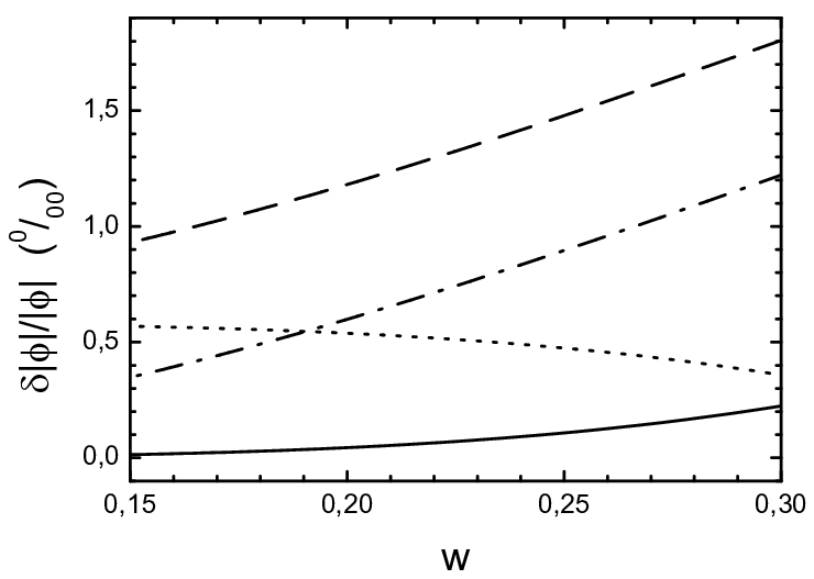
Consequently, the condition $w<1$ is well satisfied during inflation and the expansions in Eq. (23) are valid. Moreover, $p\simeq 0.0512\ll 1$ for the values in Eq. (46) and, thus, for $\lambda\sim\kappa$, the expansions in Eq. (31) are also justified. We find numerically that these expansions are, actually, justified in the entire range $w\leq w_{\max}$ even for values of $p$ close to unity and $\lambda>\kappa$. Rough estimates of the maximum relative errors when only the leading order term is kept in the expansions of Eq. (31) are given by the second term in the parentheses in this equation for $w=w_{\max}$. For the values in Eq. (46), we get that the maximum relative error in $|\phi|$, which seems to be the largest of the errors in $|\phi|$, $|\bar{\phi}|$, and $|H^{c}|$, is given by the estimate

This is verified numerically as shown in Fig. 1, where we plot the relative error in $|\phi|$ during inflation when we approximate the new smooth inflationary path by the expansions in Eq. (23). Note that, in order to retain a precision better than $1\%$ in $|\phi|$ keeping only the leading order term in its expansion in Eq. (31), the relation $M\mbox{\raisebox{-3.87495pt}{~$\stackrel{{\scriptstyle\mbox{$<$}}}{{\sim}}$~}}v_{g}/2$ has to hold, as can be seen from Eq. (49) for $w_{\max}\simeq 0.3$.

The identification of $v_{g}$, which is the VEV $|\langle H^{c}\rangle|$ or $|\langle\bar{H}^{c}\rangle|$, with the SUSY GUT scale $M_{\rm GUT}$ can be easily justified. As already mentioned, the VEVs of $H^{c}$, $\bar{H}^{c}$ break the PS gauge group to $G_{\rm SM}$, whereas the VEV of the field $\phi$ breaks it only to $G_{\rm SM}\times{\rm U}(1)_{B-L}$. So, the gauge boson $A^{\perp}$ corresponding to the linear combination of ${\rm U}(1)_{Y}$ and ${\rm U}(1)_{B-L}$ which is perpendicular to ${\rm U}(1)_{Y}$ acquires its mass squared $m^{2}_{A^{\perp}}=(5/2)g^{2}|\langle H^{c}\rangle|^{2}$ solely from the VEVs of $H^{c}$, $\bar{H}^{c}$ ($g$ is the SUSY GUT gauge coupling constant). On the other hand, the masses squared $m_{A}^{2}$ and $m_{W_{\rm R}}^{2}$ of the color triplet, anti-triplet ($A^{\pm}$) and charged ${\rm SU}(2)_{\rm R}$ ($W^{\pm}_{\rm R}$) gauge bosons get contributions from $\langle\phi\rangle$ too. Namely, $m_{A}^{2}=g^{2}(|\langle H^{c}\rangle|^{2}+(4/3)|\langle\phi\rangle|^{2})$ and $m_{W_{\rm R}}^{2}=g^{2}(|\langle H^{c}\rangle|^{2}+2|\langle\phi\rangle|^{2})$. For the values in Eq. (46), however,

which implies that $m_{A}\approx m_{W_{\rm R}}\approx gv_{g}$ within a few per cent. So, $v_{g}$ is approximately equal to the practically common mass of the SM non-singlet superheavy gauge bosons divided by $g\approx 0.7$, which is, in turn, equal to $M_{\rm GUT}\simeq 2.86\,\cdot 10^{16}\,\text{GeV}$ (the SM singlet gauge boson $A^{\perp}$ does not affect the renormalization group equations).

We will now turn to the case of a non-vanishing, but small value of the parameter $\gamma$. The scalar potential, in this case, takes the form

and the SUSY vacua lie at

Again, the vanishing of the D-terms yields $\bar{H}^{c*}=e^{i\theta}H^{c}$, which implies that we have four distinct SUSY vacua:

with $\bar{\phi}=S=0$. Here $H^{c}$, $\bar{H}^{c}$ are rotated to the real axis, but we should again keep in mind that the two vacua in Eq. (54) or (55) belong, in reality, to a continuum of vacua. One can show that the potential now generally possesses three flat directions. The first one is the usual trivial flat direction at $\phi=\bar{\phi}=H^{c}=\bar{H}^{c}=0$ with $V=V_{\rm tr}=\kappa^{2}M^{4}$. The second one exists only if $\tilde{\mu}^{2}>0$ and lies at

It is a shifted flat direction with $V=\kappa^{2}(M^{4}-\tilde{\mu}^{4})$ along which $G_{\rm PS}$ is broken to $G_{\rm SM}\times{\rm U}(1)_{B-L}$. Note that the positions of the trivial and shifted flat directions remain the same as in the $\gamma=0$ case. The third flat direction, which appears at

exists only for $\gamma\neq 0$ and is analogous to the trajectory for the new shifted hybrid inflation of Ref. nshift. Along this direction, $G_{\rm PS}$ is broken to $G_{\rm SM}$. In our subsequent discussion, we will again concentrate on the case where $\mu^{2}=-\tilde{\mu}^{2}>0$. It is interesting to note that, in this case, we always have $V_{\text{nsh}}>V_{\rm tr}$ and it is, thus, more likely that the system will eventually settle down on the trivial rather than the new shifted flat direction (the shifted flat direction in Eq. (56) does not exist in this case).

If we expand the complex scalar fields $\phi$, $\bar{\phi}$, $H^{c}$, $\bar{H}^{c}$ in real and imaginary parts according to the prescription $s=(s_{1}+i\,s_{2})/\sqrt{2}$, we find that, on the trivial flat direction, the mass-squared matrices $M_{\phi 1}^{2}$ of $\phi_{1}$, $\bar{\phi}_{1}$ and $M_{\phi 2}^{2}$ of $\phi_{2}$, $\bar{\phi}_{2}$ are

References

- (1) A.H. Guth, Phys. Rev. D 23, 347 (1981).
- (2) G. Lazarides, Lect. Notes Phys. 592, 351 (2002), hep-ph/0111328; J. Phys. Conf. Ser. 53, 528 (2006), hep-ph/0607032.
- (3) A.D. Linde, Phys. Rev. D 49, 748 (1994).
- (4) E.J. Copeland, A.R. Liddle, D.H. Lyth, E.D. Stewart, and D. Wands, Phys. Rev. D 49, 6410 (1994).
- (5) G.R. Dvali, Q. Shafi, and R.K. Schaefer, Phys. Rev. Lett. 73, 1886 (1994); G. Lazarides, R.K. Schaefer, and Q. Shafi, Phys. Rev. D 56, 1324 (1997).
- (6) J.C. Pati and A. Salam, Phys. Rev. D 10, 275 (1974).
- (7) G. Lazarides and C. Panagiotakopoulos, Phys. Lett. B 337, 90 (1994); S. Khalil, G. Lazarides, and C. Pallis, ibid. 508, 327 (2001).
- (8) B. Ananthanarayan, G. Lazarides, and Q. Shafi, Phys. Rev. D 44, 1613 (1991); Phys. Lett. B 300, 245 (1993).
- (9) G. Shiu and S.-H.H. Tye, Phys. Rev. D 58, 106007 (1998).
- (10) L.L. Everett, G.L. Kane, S.F. King, S. Rigolin, and L.-T. Wang, Phys. Lett. B 531, 263 (2002).
- (11) I. Antoniadis and G.K. Leontaris, Phys. Lett. B 216, 333 (1989); I. Antoniadis, G.K. Leontaris, and J. Rizos, ibid. 245, 161 (1990).
- (12) G. Lazarides and C. Panagiotakopoulos, Phys. Rev. D 52, R559 (1995); G. Lazarides, C. Panagiotakopoulos, and N.D. Vlachos, ibid. 54, 1369 (1996); R. Jeannerot, S. Khalil, and G. Lazarides, Phys. Lett. B 506, 344 (2001).
- (13) G. Lazarides, M. Magg, and Q. Shafi, Phys. Lett. B 97, 87 (1980).
- (14) R. Jeannerot, S. Khalil, G. Lazarides, and Q. Shafi, J. High Energy Phys. 10, 012 (2000).
- (15) G. Lazarides, hep-ph/0011130; R. Jeannerot, S. Khalil, and G. Lazarides, hep-ph/0106035.
- (16) R. Jeannerot, S. Khalil, and G. Lazarides, J. High Energy Phys. 07, 069 (2002).
- (17) M.E. Gomez, G. Lazarides, and C. Pallis, Nucl. Phys. B638, 165 (2002).
- (18) G. Lazarides and C. Pallis, hep-ph/0404266; hep- ph/0406081.
- (19) R. Hempfling, Phys. Rev. D 49, 6168 (1994); L.J. Hall, R. Rattazzi, and U. Sarid, ibid. 50, 7048 (1994).
- (20) G. Lazarides, Q. Shafi, and C. Wetterich, Nucl. Phys. B181, 287 (1981); G. Lazarides and Q. Shafi, ibid. B350, 179 (1991).
- (21) M.E. Gomez, G. Lazarides, and C. Pallis, Phys. Rev. D 67, 097701 (2003).
- (22) D.N. Spergel et al., Astrophys. J. Suppl. Ser. 170, 377 (2007).
- (23) V.N. Şenoğuz and Q. Shafi, Phys. Lett. B 567, 79 (2003).
- (24) O. Seto and J. Yokoyama, Phys. Rev. D 73, 023508 (2006).
- (25) M. Bastero-Gil, S.F. King, and Q. Shafi, Phys. Lett. B 651, 345 (2007).
- (26) M. ur Rehman, V.N. Şenoğuz, and Q. Shafi, Phys. Rev. D 75, 043522 (2007).
- (27) L. Boubekeur and D. Lyth, J. Cosmol. Astropart. Phys. 07, 010 (2005).
- (28) B. Garbrecht, C. Pallis, and A. Pilaftsis, J. High Energy Phys. 12, 038 (2006).
- (29) V.N. Şenoğuz and Q. Shafi, Phys. Rev. D 71, 043514 (2005); hep-ph/0512170.
- (30) B.A. Bassett, S. Tsujikawa, and D. Wands, Rev. Mod. Phys. 78, 537 (2006).
- (31) M.Yu. Khlopov and A.D. Linde, Phys. Lett. B 138, 265 (1984); J. Ellis, J.E. Kim, and D. Nanopoulos, ibid. 145, 181 (1984); J.R. Ellis, D.V. Nanopoulos, and S. Sarkar, Nucl. Phys. B259, 175 (1985).