跳到论文正文
W Papers独立论文阅读器 arXiv:0705.3764 论文正文 计算阅读时间 · 0%
引用这篇论文根据当前论文元数据生成,正式投稿前建议核对。


License: Assumed arXiv.org perpetual non-exclusive license
arXiv:0705.3764v1 [gr-qc] 24 May 2007

Semiclassical Approximations to Cosmological Perturbations

Mattia Luzzi

   Università degli Studi di Bologna   FACOLTÀ DI SCIENZE MATEMATICHE, FISICHE E NATURALI

Dottorato di Ricerca in Fisica

Semiclassical Approximations to Cosmological Perturbations

Tesi di Dottorato di: Relatore: Chiar.mo

Mattia Luzzi Prof. Giovanni Venturi

Corelatori:

Dott. Roberto Casadio

Dott. Fabio Finelli

Dott. Alexander Kamenshchik

Sigla del Settore Scientifico Disciplinare: FIS/02

Visto del Coordinatore di Dottorato, Prof. Fabio Ortolani

XIX   Ciclo

       Anno Accademico 2005-2006      

“Would you tell me, please, which way I ought go from here?”
“That depends a good deal on where you want to get to”, said the Cat.
“I don’t much care where -” said Alice.
“Then it doesn’t matter which way you go,” said the Cat.
“- so long as I get somewhere,” Alice added as an explanation.
“Oh, you’re sure to do that,” said the Cat, “if you only walk long enough.”

from “Alice’s Adventures in Wonderland” by Lewis Carroll

I would like to thank my supervisor Prof. Giovanni Venturi for his support and encouragement. I would also like to thank the whole INFN Bologna group BO11. I warmly thank Dr. Roberto Casadio for being always so kind and ready–to–help me in any respect. For the many interactions I had and specially for the fact that working with them was lots of fun, I want to express my acknowledgement to Dr. Fabio Finelli and Dr. Alexander Kamenshchik. Our fruitful collaboration forms the basis of much of the work presented here.

SEMICLASSICAL APPROXIMATIONS TO COSMOLOGICAL PERTURBATIONS

Mattia Luzzi

Index

Introduction

One of the main ideas of modern cosmology is that there was an epoch in the history of the Universe when vacuum energy dominated other forms of energy density such as radiation or matter. During this vacuum-dominated (or potential-dominated) era, the scale factor grew exponentially (or almost exponentially) in time and, for this reason, it is known as inflation. During inflation, a small and smooth spatial region of size less than the Hubble radius at that time could have grown so large to easily encompass the comoving volume of the entire Universe presently observable. If the early Universe underwent a period of so rapid expansion, one can then understand why the observed Universe is homogeneous and isotropic to such a high accuracy. All these virtues of inflation were already noted when it was first proposed in a seminal paper by Guth in 1981 [1]. Other, and more dramatic consequences of the inflationary paradigm were discovered soon after. Starting with a Universe which is absolutely homogeneous and isotropic at the classical level, the inflationary expansion will “freeze in” the vacuum fluctuations of the “inflaton” (the field responsible for the rapid expansion) which then becomes a classical quantity. On each comoving scale, this happens soon after the fluctuation exits the Hubble horizon. A primordial energy density, which survives after the end of inflation, is associated with these vacuum fluctuations and may be responsible for both the anisotropies in the Cosmic Microwave Background (CMB) and for the large-scale structures of the Universe, like galaxies, clusters of galaxies, and dark matter. Inflation also generates primordial gravitational waves, which may contribute to the low multipoles of the CMB anisotropy. The amazing prediction of inflation is therefore that all of the structures we see in the present Universe are the result of quantum-mechanical fluctuations during the inflationary epoch.

Units and Conventions

The so–called natural units, namely ℏ=c=1\hbar=c=1, will be employed, so that

[Energy]=[Mass]=[Length]−1=[Time]−1.[{\rm Energy}]=[{\rm Mass}]=[{\rm Length}]^{-1}=[{\rm Time}]^{-1}~.

mPl=1/Gm_{\rm Pl}=1/\sqrt{G} is the Planck mass, whereas MPl=1/8​π​GM_{\rm Pl}=1/\sqrt{8\,\pi\,G} stands for the reduced Planck mass, and ℓPl=8​π​MPl−1\ell_{\rm Pl}=\sqrt{8\,\pi}\,M^{-1}_{\rm Pl} is the Planck length. The present Hubble expansion rate is customarily parameterised as H0=100​h​km​sec−1​Mpc−1H_{0}=100\,h\,{\rm km}\,{\rm sec}^{-1}\,{\rm Mpc}^{-1} where hh parameterises the uncertainty in the present value of the Hubble parameter.

We shall also adopt the Einstein sum rule for repeated indices and the following conventions: The metric signature is (+,−,−,−+,-,-,-), Greek letters denote space-time indices which run from 0 to 3 and Latin letters denote spatial indices which run from 1 to 3.

Some abbreviations used in this thesis are the following:

CMB = Cosmic Microwave Background

EW = electroweak

BBN = Big Bang Nucleosintesis

GR = General Relativity

COBE = COsmic Background Explorer satellite

DMR = Differential Microwave Radiometer

WMAP = Wilkinson Microwave Anisotropy Probe

ACBAR = Arcminute Cosmology Bolometer Array Receiver

VSA = Very Small Array

CBI = Cosmic Background Imager

Λ\Lambda CDM = Λ\LambdaCold Dark Matter

FRW= Friedmann-Robertson-Walker

WKB = Wentzel-Kramers-Brillouin

MCE = Method of Comparison Equation

PS = Power Spectrum

HFF = Horizon Flow Functions

SR = Slow Roll

HSR = Hubble Slow Roll

PSR = Hubble Slow Roll

GFM = Green Function Method

Chapter 1 What’s the matter?

What is the origin of the inhomogeneities we observe in the sky? What is their typical wavelength? How come that we are able to observe these inhomogeneities? The term inhomogeneity is rather generic and indicates fluctuations both in the background geometry and in the energy content of the Universe. These inhomogeneities can be represented by plane waves characterized by a comoving wave-number kk. Since the evolution of the Universe is characterized by a scale factor a⁡(t)a(t) which is a function of the cosmic time tt, the physical wave-number is given by kph=k/ak_{\rm ph}=k/a. The comoving wave-number is a constant and does not feel the expansion of the Universe, while the physical momentum is different at different epochs. Conversely the value of a given physical frequency is fully specified only by stating the time at which the physical frequency is “measured”.

For example, if a given fluctuation has a momentum comparable with the present value of the Hubble parameter, kph,0≃H0≃5.6×10−61​MPlk_{{\rm ph,}0}\simeq H_{0}\simeq 5.6\times 10^{-61}\,M_{\rm Pl}, we will have that kph,0≃2.3×10⁻¹⁸k_{{\rm ph,}0}\simeq 2.3\times 10^{-18} Hz. Fluctuations with momentum smaller that H0H_{0} have a wave-length larger than the present value of the Hubble radius and are therefore impossible to detect directly since the distance between two of their maxima (or minima) is larger than our observable Universe.

At the decoupling epoch, when the radiation became free to propagate, the temperature of the Universe was of the order of a fraction of eV{\rm eV} and the Hubble rate was Hdec≃6.7×10−56​MPlH_{\rm dec}\simeq 6.7\times 10^{-56}\,M_{\rm Pl}. The corresponding decoupling frequency was then red-shifted to the present value kph,dec≃3×10⁻¹⁶​Hzk_{\rm ph,dec}\simeq 3\times 10^{-16}\,{\rm Hz}. Fluctuations of this typical frequency appear as temperature inhomogeneities of the CMB induced by the primordial fluctuations in the background geometry and in the matter density. The latter fluctuations have already collapsed due to gravitational instability and formed galaxies and clusters of galaxies. At the epoch of the formation of light nuclei, the Universe was hotter, with a temperature of a fraction of MeV{\rm MeV} and the corresponding value of the Hubble expansion rate was about 8×10−44​MPl8\times 10^{-44}\,M_{\rm Pl}. When the electroweak (EW) phase transition took place, the temperature of the Universe was of the order of 100​GeV100\,{\rm GeV} leading, approximately, to HEW∼10−32​MPlH_{\rm EW}\sim 10^{-32}\,M_{\rm Pl}. Comoving wave-numbers of the order of the Hubble rate at the EW phase transition or at the epoch of the Big Bang Nucleosintesis (BBN) correspond, today, to physical frequencies of the order of kph,EW∼2×10⁻⁵​Hzk_{\rm ph,EW}\sim 2\times 10^{-5}\,{\rm Hz} or kph,BBN≃9×10⁻¹¹​Hzk_{\rm ph,BBN}\simeq 9\times 10^{-11}\,{\rm Hz}. Finally, in the context of the inflationary paradigm the value of the Hubble rate during inflation was Hinf∼10−6​MPlH_{\rm inf}\sim 10^{-6}\,M_{\rm Pl}. Under the assumption that the Universe was dominated by radiation right after inflation, the corresponding physical frequency today is of the order of 10810^{8}\,Hz.

The detectors developed to measure anisotropies in the CMB are sensitive to frequency scales only slightly higher than 10−1610^{-16}\,Hz. Therefore, they cannot be used to “observe” fluctuations originated at earlier epochs and whose physical frequencies presently lie in the range 10−3​Hz<kph<1​MHz10^{-3}\,{\rm Hz}<k_{\rm ph}<1\,{\rm MHz}. For frequencies in this interval, one can only hope to detect the stochastic background of gravitational radiation which is therefore the only means we have to obtain direct information about the EW phase transition, the BBN and inflation itself.

The cosmological inhomogeneities are usually characterized by their correlation functions. The simplest correlation function encoding informations on the nature of the fluctuations is the two-point function which is computed by taking averages of the fluctuation amplitude at two spatially separated points but at the same time. Its Fourier transform is usually called the power spectrum. On considering the physical scales discussed above, one is led to conclude that the power spectrum of cosmological inhomogeneities is defined over a huge interval of frequencies. For instance, the tensor fluctuations of the geometry, which only couple to the curvature and not to the matter sources, have a spectrum ranging, in some specific models, from 10−1810^{-18}\,Hz up to about 11\,GHz.

From the history of the Universe sketched so far, some questions may be naturally raised. For our purposes, we just quote two of them:

  • •

    Given that the precise thermodynamical history of the Universe above 1010\,MeV is unknown, how it is possible to have a reliable framework describing the evolution of the cosmological fluctuations?

  • •

    Does it make sense to apply General Relativity (GR) to curvatures which can reach up to almost the Planck scale?

As recalled above, we do not have any direct evidence for the thermodynamical state of the Universe for temperatures above the MeV, although some indirect predictions can be made. For example, the four lighter isotopes (D{\rm D}, He3{}^{3}{\rm He}, He4{}^{4}{\rm He} and Li7{}^{7}{\rm Li}) should have been mainly produced at the BBN below a typical temperature of 0.80.8\,MeV when neutrinos decouple from the plasma and the neutron abundance evolves via free neutron decay. The abundances calculated in the homogeneous and isotropic BBN model agree fairly well with the astronomical observations. This is the last indirect test of the thermodynamical state of the Universe. For temperatures larger than 1010\,MeV, collider physics and the success of the standard model of particle physics offer a precious handle up to the epoch of the EW phase transition occurring for temperatures of the order of 100100\,GeV. There is then hope that our knowledge of particle physics could help us to fill the gap between the epoch of nucleosynthesis and that of the EW phase transition.

The evolution of inhomogeneities over cosmological distances may well be unaffected by our ignorance of the specific history of the expansion rate. The key concept is that of conservation laws and, in the framework of metric theories of gravity (and of GR in particular), one can show that there exist conservation laws for the evolution of the fluctuations which become exact in the limit of vanishing comoving frequency k→0k\to 0. This conclusion holds under the assumption that GR is a valid description throughout the whole evolution of the Universe and similar properties also hold, with some modifications, in scalar-tensor theories of gravity (of the Brans-Dicke type) like those suggested by the low-energy limit of superstring theory. The conservation laws of cosmological perturbations apply strictly in the case of the tensor modes of the geometry whereas, for scalar fluctuations which couple directly to the (scalar) matter sources, the precise form of the conservation laws depends upon the matter content of the early Universe. Experiments aimed at the direct detection of stochastic backgrounds of relic gravitons which regard the high-frequency behaviour of cosmological fluctuations should therefore yield valuable clues on the early evolution of the Hubble rate.

1.1 A short (incomplete) introduction to a long history

The history of the studies about the CMB anisotropies and cosmological fluctuations is closely related with the history of the standard cosmological model (see, for instance, the textbooks by Weinberg [2] and Kolb and Turner [3]).

During the development of the standard model of cosmology, one of the recurrent issues has been the explanation of the structures we observe in the present Universe, which goes under the name of the structure formation. The reviews of Kodama and Sasaki [4] and of Mukhanov, Feldman and Brandenberger [5] contain some historical surveys that are a valuable introduction to this subject.

A seminal contribution to the understanding of cosmological perturbations is the paper of Sachs and Wolfe [6] on the possible generation of anisotropies in the CMB, where the basic general relativistic effects were estimated assuming that the CMB itself was of cosmological origin. The authors argued that galaxy formation would imply Δ​T/T∼10−2\Delta T/T\sim 10^{-2}. Subsequent calculations [7, 8, 9, 10, 11] brought the estimate down to 10−410^{-4}, closer to what is experimentally observed. A second foundamental paper is the contribution of Sakharov [12] where the concept of acoustic oscillations was introduced. This paper contained two ideas whose legacy, somehow unexpectedly, survived until the present. The first idea is summarized in the abstract

A hypothesis of the creation of astronomical bodies as a result of gravitational instability of the expanding Universe is investigated. It is assumed that the initial inhomogeneities arise as a result of quantum fluctuations…

The model indeed assumed that the initial state of the baryon-lepton fluid was cold. So the premise was wrong, but, still, it is amusing to notice that a variety of models today assume quantum fluctuations as initial conditions for the fluctuations of the geometry at a totally different curvature (or energy).

To summarise, Refs. [6] and [12] highlight three important problems regarding the fluctuations of the gravitational inhomogeneities:

  • •

    their initial conditions;

  • •

    their evolution;

  • •

    their imprint on the CMB temperature fluctuations.

1.2 CMB experiments

Although we shall just study a particular aspect of the theory of cosmological perturbations, it is appropriate to give a swift account of our recent experimental knowledge of CMB anisotropies. A new twist in the study of CMB anisotropies came from the observations of the COsmic Background Explorer satellite (COBE) and, more precisely, from the Differential Microwave Radiometer (DMR). The DMR was able to probe the angular power spectrum CℓC_{\ell} 11 1 We just recall here that ℓ⁡(ℓ+1)​Cℓ/(2​π)\ell(\ell+1)\,C_{\ell}/(2\,\pi) measures the degree of inhomogeneity in the temperature distribution per logarithmic interval of ℓ\ell. Consequently, a given multipole ℓ\ell can be related to a given spatial structure in the microwave sky: small ℓ\ell will correspond to smaller and high ℓ\ell to larger wave-numbers around a present physical frequency of the order of 10−1610^{-16} Hz. up to ℓ≃25\ell\simeq 25 (see, for instance, [13, 14] and references therein). DMR was a differential instrument measuring temperature differences in the microwave sky. The angular separation ϑ\vartheta of the two horns of the antenna is related to the largest multipole according to the approximate relation ϑ≃π/ℓ\vartheta\simeq\pi/\ell.

COBE explored angular separations ϑ≳70\vartheta\gtrsim 7^{0} and, after the COBE mission, various experiments have probed smaller angular separation, i.e., larger multipoles. A finally convincing evidence of the existence and location of the first peak in CℓC_{\ell} came from Boomerang [15, 16], Maxima [17] and Dasi [18]. These last three experiments explored multipoles up to ℓ=1000\ell=1000, determining the first acoustic oscillation for ℓ≃220\ell\simeq 220. Another important experiment was Archeops [19] providing interesting data for the region characterizing the first rise of the angular spectrum.

Refer to caption
Figure 1.1: Some of the most recent CMB anisotropy data from [20]: WMAP (filled circles); VSA (shaded circles) [20]; CBI (squares) [21, 22] and ACBAR (triangles) [23].

The angular spectrum, as measured by different recent experiments is reported in Fig. 1.1. The data from the Wilkinson Microwave Anisotropy Probe (WMAP) are displayed as filled circles in Fig. 1.1 and provide, among other important evidences, a precise determination of the position of the first peak (i.e., ℓ=220.1±0.8\ell=220.1\pm 0.8 [24]) and a clear evidence of the second peak. Further, once all the four-years data are collected, the spectrum will be obtained with good resolution up to ℓ∼1000\ell\sim 1000, i.e., around the third peak. In Fig. 1.1, we also display the results of the Arcminute Cosmology Bolometer Array Receiver (ACBAR) as well as the data points of the Very Small Array (VSA) and of the Cosmic Background Imager (CBI).

In recent years, thanks to the combined observations of CMB anisotropies [25], Large scale structure [26, 27], supernovae of type Ia, BBN [28], some kind of paradigm for the evolution of the late time (or even present) Universe has emerged. This is normally called Λ\LambdaCold Dark Matter (Λ\Lambda CDM) model or, sometimes, “concordance model”. The term Λ\LambdaCDM refers to the fact that, in this model, the dominant (present) component of the energy density of the Universe is given by a cosmological constant Λ\Lambda and a fluid of cold dark matter particles interacting only gravitationally with the other (known) particle species such as baryons, leptons, photons. According to this paradigm, our understanding of the Universe can be summarized in two sets of cosmological parameters, one referring to the homogeneous background and one to the inhomogeneities. As far as the homogeneous background is concerned, the most important parameter is the indetermination on the (present) Hubble expansion rate which is customarily parameterised as H0=h×100​km/[sec×Mpc]H_{0}=h\times 100{\rm km}/[{\rm sec}\times{\rm Mpc}] (h≃0.72h\simeq 0.72 in the concordance model). There are various other parameters, such as the dark and CDM energy densities in critical units, Ωcdm≃0.224\Omega_{\rm cdm}\simeq 0.224 and ΩΛ≃0.73\Omega_{\Lambda}\simeq 0.73, respectively; the radiation and baryon energy densities in critical units, Ωr≃8×10⁻⁵\Omega_{\rm r}\simeq 8\times 10^{-5} and Ωb≃0.046\Omega_{\rm b}\simeq 0.046; the number of neutrino species and their masses; the possible contribution of the spatial curvature (Ωκ=0\Omega_{\kappa}=0 in the concordance model) the optical depth of the plasma at recombination (of the order of 0.160.16 in the concordance model).

The second set of parameters refers to the inhomogeneities. In the Λ\LambdaCDM model the initial conditions for the inhomogeneities belong to a specific class of scalar fluctuations of the geometry which are called adiabatic and are characterized by the Fourier transform of their two-point function. This is the power spectrum which is usually parametrized in terms of an amplitude and a spectral slope. Besides these two parameters, one usually considers the ratio between the amplitudes of the scalar and tensor modes of the geometry.

The purpose of this thesis is to report the development of a method for the resolution of the differential equation that drives the modes of scalar and tensorial perturbations of the cosmological inhomogeneities. This work is organized as follows: in Chapter 2 we review the Friedmann-Robertson-Walker (FRW) space-time and remark some aspects about gauge choices. Chapter 3 deals with the process of generation of cosmological perturbations by quantum fluctuations of a scalar field and a second-order differential equation for the quantities of interest is obtained. Such a kind of equations will be treated with semiclassical approximations in Chapter 4. In Chapter 5 we give new general results for the power spectra of cosmological perturbations, while in Chapter 6 we use those results to find, in detail, explicit expressions for the power spectra in several inflationary models. The thesis ends with our Conclusions and several Appendicies.

Chapter 2 FRW Universes and their inhomogeneities

2.1 FRW Universes

A Friedmann-Robertson-Walker (FRW) metric can be written in terms of the cosmic time tt as

gμ​ν(0)​d​xμ​d​xν=d​t2−a2​(t)​[d​r21−κ​r2+r2​(d​θ2+sin2⁡θ​d​φ2)],{}^{(0)}g_{\mu\,\nu}\,\mbox{${\rm d}$}x^{\mu}\,\mbox{${\rm d}$}x^{\nu}=\mbox{${\rm d}$}t^{2}-a^{2}(t)\,\left[\frac{\mbox{${\rm d}$}r^{2}}{1-\kappa\,r^{2}}+r^{2}\,\left(\mbox{${\rm d}$}\theta^{2}+\sin^{2}{\theta}\mbox{${\rm d}$}\varphi^{2}\right)\right]\ , (2.1)

where κ\kappa can be 11, 00 and −1-1 for spherical, eucledian or hyperbolic spatial sections, respectively; aa is the scale factor, while r,θ,φr,\theta,\varphi are the spherical coordinates. We can also write the metric in terms of the conformal time η\eta, defined by d​η≡d​t/a⁡(t)\mbox{${\rm d}$}\eta\equiv\mbox{${\rm d}$}t/a(t), as

gμ​ν(0)​d​xμ​d​xν=a2​(η)​{d​η2−[d​r21−κ​r2+r2​(d​θ2+sin2⁡θ​d​φ2)]}.{}^{(0)}g_{\mu\,\nu}\,\mbox{${\rm d}$}x^{\mu}\,\mbox{${\rm d}$}x^{\nu}=a^{2}(\eta)\,\left\{\mbox{${\rm d}$}\eta^{2}-\left[\frac{\mbox{${\rm d}$}r^{2}}{1-\kappa\,r^{2}}+r^{2}\,\left(\mbox{${\rm d}$}\theta^{2}+\sin^{2}{\theta}\mbox{${\rm d}$}\varphi^{2}\right)\right]\right\}\ . (2.2)

The evolution of the geometry is driven by the matter sources according to the Einstein equations

Gμ​ν≡Rμ​ν−12​δμ​ν​R=8​π​G​Tμ​ν,\displaystyle G_{\mu\,\nu}\equiv R_{\mu\,\nu}-\frac{1}{2}\,\delta_{\mu\,\nu}\,R=8\,\pi\,G\,T_{\mu\,\nu}\ , (2.3)

where Gμ​νG_{\mu\nu} is the Einstein tensor, Rμ​νR_{\mu\nu} and RR are the Ricci tensor and Ricci scalar, respectively; Tμ​νT_{\mu\nu} is the energy-momentum tensor of the sources. Under the hypothesis of homogeneity and isotropy, we can always write the energy-momentum tensor in the form Tμ​ν=diag⁡(ρ,p,p,p)T_{\mu\nu}={\rm diag}\left(\rho,p,p,p\right) where ρ\rho is the energy density of the system and pp its pressure and are functions of the time. Using Eq. (2.3) we obtain the Friedmann equations which, in conformal time, read

ℋ2=8​π​G​ρ​a23−κ,ℋ′=−4​π​G3​(ρ+3​p)​a2\displaystyle{\cal H}^{2}=\frac{8\,\pi\,G\,\rho\,a^{2}}{3}-\kappa\ ,\quad{\cal H}^{\prime}=-\frac{4\,\pi\,G}{3}\,\left(\rho+3\,p\right)\,a^{2} (2.4)

along with the continuity equation

ρ′+3​ℋ​(ρ+p)=0.\displaystyle\rho^{\prime}+3{\cal H}\,(\rho+p)=0\ . (2.5)

In the above formulae ℋ≡a′/a{\cal H}\equiv a^{\prime}/a and a prime denotes a derivation with respect to the conformal time. In cosmic time, the same equations become

H2=8​π​G​ρ3−κa2,H˙=− 4​π​G​(ρ+p)+κa2\displaystyle H^{2}=\frac{8\,\pi\,G\,\rho}{3}-\frac{\kappa}{a^{2}}\ ,\quad\dot{H}=-\,4\,\pi\,G\,\left(\rho+p\right)+\frac{\kappa}{a^{2}} (2.6)

and the continuity equation is given by

ρ˙+3​H​(ρ+p)=0,\displaystyle\dot{\rho}+3\,H\,(\rho+p)=0\ , (2.7)

where H≡a˙/aH\equiv\dot{a}/a is the Hubble expansion rate and dot denotes a derivation with respect to tt. The relation between the Hubble factors in the two time parametrizations is ℋ=a​H{\cal H}=a\,H.

2.2 Fluctuations of the geometry in flat FRW Universes

Let us now consider a conformally flat (i.e., κ=0\kappa=0) background metric of FRW type,

gμ​ν​(η)=a2​(η)​ημ​ν,\displaystyle g_{\mu\nu}(\eta)=a^{2}(\eta)\,\eta_{\mu\nu}\ , (2.8)

where ημ​ν\eta_{\mu\nu} is the flat Minkowski metric. Its first-order fluctuations can be written as

δ​gμ​ν​(η,x→)=δs​gμ​ν​(η,x→)+δv​gμ​ν​(η,x→)+δt​gμ​ν​(η,x→),\displaystyle\delta\,g_{\mu\nu}(\eta,\vec{x})=\delta_{\rm s}\,g_{\mu\nu}(\eta,\vec{x})+\delta_{\rm v}\,g_{\mu\nu}(\eta,\vec{x})+\delta_{\rm t}\,g_{\mu\nu}(\eta,\vec{x})\ , (2.9)

where the subscripts define, respectively, the scalar, vector and tensor perturbations. The perturbed metric δ​gμ​ν\delta\,g_{\mu\nu} has ten independent components whose explicit form can be parametrized as

δ​g00\displaystyle\delta\,g_{00} =\displaystyle= 2​a2​ϕ\displaystyle 2\,a^{2}\,\phi
δ​gi​j\displaystyle\delta\,g_{ij} =\displaystyle= 2​a2​(ψ​δi​j−∂i∂jE)−a2​hi​j−a2​(∂iFj+∂jFi)\displaystyle 2\,a^{2}\,\left(\psi\,\delta_{ij}-\partial_{i}\,\partial_{j}\,E\right)-a^{2}\,h_{ij}-a^{2}\,\left(\partial_{i}\,F_{j}+\partial_{j}\,F_{i}\right)
δ​g0​i\displaystyle\delta\,g_{0i} =\displaystyle= −a2∂iB+a2Si,\displaystyle-a^{2}\,\partial_{i}\,B+a^{2}\,S_{i}\ , (2.10)

with the conditions

∂iSi=∂iFi=0,hii=∂ihji=0.\displaystyle\partial_{i}\,S^{i}=\partial_{i}\,F^{i}=0\ ,\quad h_{i}^{i}=\partial_{i}\,h^{i}_{j}=0\ . (2.11)

The decomposition given in Eqs. (2.10) is that normally employed in the Bardeen formalism [29] (see Ref. [5]).

The scalar fluctuations are parametrized by the scalar functions ϕ\phi, ψ\psi, BB and EE. The vector fluctuations are described by two divergenceless (see Eqs. (2.11)) vectors in three (spatial) dimensions FiF_{i} and SiS_{i} (i.e., by four independent degrees of freedom). Finally the tensor modes are described by hi​jh_{ij}, leading to two independent components (see Eqs. (2.11)).

Under general infinitesimal coordinate transformations

η→η~=η+ϵ0,xi→x~i=xi+ϵi\displaystyle\eta\to\tilde{\eta}=\eta+\epsilon_{0}\ ,\quad{x}^{i}\to\tilde{x}^{i}=x^{i}+\epsilon^{i} (2.12)

the fluctuations of the geometry defined in Eqs. (2.10) transform as

δ​gμ​ν→δ​g~μ​ν=δ​gμ​ν−∇μϵν−∇νϵμ,\displaystyle\delta\,{g}_{\mu\nu}\to\delta\,\tilde{g}_{\mu\nu}=\delta\,g_{\mu\nu}-\nabla_{\mu}\,\epsilon_{\nu}-\nabla_{\nu}\,\epsilon_{\mu}\ , (2.13)

where ∇μ\nabla_{\mu} is the covariant derivative with respect to the background goemetry and ϵμ=a2​(η)​(ϵ0,−ϵi)\epsilon_{\mu}=a^{2}(\eta)\left(\epsilon_{0},-\epsilon_{i}\right). These infinitesimal coordinate transformations form a group and the functions ϵ0\epsilon_{0} and ϵi\epsilon_{i} are the gauge parameters. The gauge-fixing procedure amounts to fixing the four gauge parameters. Further, the spatial components ϵi\epsilon_{i} can be separated into divergenceless and divergencefull parts

ϵi=∂iϵ+ζi,\displaystyle\epsilon_{i}=\partial_{i}\,\epsilon+\zeta_{i}\ , (2.14)

where ∂iζi=0\partial_{i}\,\zeta^{i}=0. The gauge transformations involving ϵ0\epsilon_{0} and ϵ\epsilon preserve the scalar nature of the fluctuations while those parametrized by ζi\zeta_{i} preserve the vector nature of the fluctuation.

The background covariant derivatives in Eq. (2.13) are given by ∇μϵν=∂μϵν−(0)Γμ​νσϵσ\nabla_{\mu}\,\epsilon_{\nu}=\partial_{\mu}\,\epsilon_{\nu}-^{(0)}\Gamma_{\mu\nu}^{\sigma}\,\epsilon_{\sigma} and, in terms of the unperturbed connections (see Eqs. (A.7)), the fluctuations for the scalar modes can be written in the tilded coordinate system as

ϕ→ϕ~=ϕ−ℋ​ϵ0−ϵ0′\displaystyle\phi\to\tilde{\phi}=\phi-{\cal H}\,\epsilon_{0}-\epsilon_{0}^{\prime} (2.15)
ψ→ψ~=ψ+ℋ​ϵ0\displaystyle\psi\to\tilde{\psi}=\psi+{\cal H}\,\epsilon_{0} (2.16)
B→B~=B+ϵ0−ϵ′\displaystyle B\to\tilde{B}=B+\epsilon_{0}-\epsilon^{\prime} (2.17)
E→E~=E−ϵ.\displaystyle E\to\tilde{E}=E-\epsilon\ . (2.18)

Under a coordinate transformation preserving the vector nature of the fluctuation, xi→x~i=xi+ζix^{i}\to\tilde{x}^{i}=x^{i}+\zeta^{i} (with ∂iζi=0\partial_{i}\,\zeta^{i}=0), the rotational modes of the geometry transform as

Si→S~i=Si+ζi′\displaystyle S_{i}\to\tilde{S}_{i}=S_{i}+\zeta_{i}^{\prime} (2.19)
Fi→F~i=Fi−ζi.\displaystyle F_{i}\to\tilde{F}_{i}=F_{i}-\zeta_{i}\ . (2.20)

Finally, the tensor fluctuations in the parametrization of Eqs. (2.10) are automatically gauge invariant.

The perturbed components of the energy-momentum tensor can be written as

δ​T00=δ​ρ,δ​Tij=−δ​p​δij,δ​T0i=(p+ρ)​∂iv,\displaystyle\delta\,T_{0}^{0}=\delta\,\rho\ ,\quad\delta\,T_{i}^{j}=-\delta\,p\,\delta_{i}^{j}\ ,\quad\delta\,T_{0}^{i}=\left(p+\rho\right)\,\partial^{i}\,v\ , (2.21)

where vv is the velocity field and δ​ui=∂iv\delta u_{i}=\partial_{i}\,v. Under the infinitesimal coordinate transformations (2.12), the fluctuations given in Eq. (2.21) transform as

δ​ρ→δ​ρ~=δ​ρ−ρ′​ϵ0\displaystyle\delta\,\rho\to\delta\,\tilde{\rho}=\delta\,\rho-\rho^{\prime}\,\epsilon_{0} (2.22)
δ​p→δ​p~=δ​p−w​ρ′​ϵ0\displaystyle\delta\,p\to\delta\,\tilde{p}=\delta\,p-w\,\rho^{\prime}\,\epsilon_{0} (2.23)
v→v~=v+ϵ′.\displaystyle v\to\tilde{v}=v+\epsilon^{\prime}\ . (2.24)

Using the covariant conservation equation (2.5) for the background fluid density, the gauge transformation for the density perturbation δ≡δ​ρ/ρ\delta\equiv\delta\,\rho/\rho follows from Eq. (2.22) and reads

δ~=δ−3​ℋ​(1+Pρ)​ϵ0.\displaystyle\tilde{\delta}=\delta-3\,{\cal H}\,\left(1+\frac{P}{\rho}\right)\,\epsilon_{0}\ . (2.25)

We now have two possible ways of proceeding:

  • •

    fix, completely or partially, the coordinate system (i.e., the gauge);

  • •

    use a gauge-invariant approach.

We shall briefly review both.

2.3 Gauge fixing and gauge-invariant variables

As we recalled above, the tensor modes are already gauge-invariant, whereas the vector and scalar modes change for infinitesimal coordinate transformations. Since the gauge fixing of the vector fluctuations is analogous, but simpler, to the one of the scalar modes, vectors will be discussed before scalars.

2.3.1 Vector modes

We have two different gauge choices for the vector modes. The first is to set S~i=0\tilde{S}_{i}=0 so that, from Eq. (2.19), we have

ζi(η,x→)=−∫ηSi(η′,x→)dη′+Ci(x→).\displaystyle\zeta_{i}(\eta,\vec{x})=-\int^{\eta}\,S_{i}(\eta^{\prime},\vec{x})\,\mbox{${\rm d}$}\eta^{\prime}+C_{i}(\vec{x})\ . (2.26)

Since the gauge function is determined up to arbitrary (space-dependent) constants CiC_{i}, the coordinate system is not completely fixed by this choice. The second choice is F~i=0\tilde{F}_{i}=0 and, from Eq. (2.20), ζi=Fi\zeta_{i}=F_{i}. The gauge freedom is therefore completely fixed in this manner.

Instead of fixing a gauge, we could work directly with gauge-invariant quantities. We note that, from Eqs. (2.19) and (2.20), the combination Fi′+SiF_{i}^{\prime}+S_{i} is invariant under infinitesimal coordinate transformations preserving the vector nature of the fluctuations. This is the vector counterpart of the Bardeen potentials [29].

2.3.2 Scalar modes

More options are available in the literature for scalar modes and we briefly review the more common ones (see Ref. [5] for more details).

Conformally Newtonian (or Longitudinal) gauge

In this gauge we eliminate all the off-diagonal entries E~\tilde{E} and B~\tilde{B} of the perturbed metric in Eq. (2.13), i.e. E~L=B~L=0\tilde{E}_{\rm L}=\tilde{B}_{\rm L}=0. From Eqs. (2.17) and (2.18) the gauge functions are then determined as ϵ=E\epsilon=E and ϵ0=E′−B\epsilon_{0}=E^{\prime}-B and the only non-vanishing entries of the perturbed metric are ϕ~\tilde{\phi} and ψ~\tilde{\psi}.

Off-diagonal (or Uniform Curvature) gauge

This gauge is characterized by the conditions E~od=0\tilde{E}_{\rm od}=0 and ψ~od=0\tilde{\psi}_{\rm od}=0. From Eqs. (2.16) and (2.18) we find ϵ0=−ψ/ℋ\epsilon_{0}=-\psi/{\cal H} and ϵ=E\epsilon=E. The two non-vanishing metric fluctuations are then B~\tilde{B} and ϕ~\tilde{\phi}. Since ψ~od=0\tilde{\psi}_{\rm od}=0, the fluctuation of the spatial curvature also vanishes.

Synchronous gauge

This coordinate system is defined by ϕ~S=B~S=0\tilde{\phi}_{\rm S}=\tilde{B}_{\rm S}=0, which however does not fix the gauge completely. In fact, Eqs. (2.15) and (2.17) imply that the gauge functions are determined by

(ϵ0​a)′=a​ϕ,ϵ′=(B+ϵ0),\displaystyle(\epsilon_{0}\,a)^{\prime}=a\,\phi\ ,\quad\epsilon^{\prime}=(B+\epsilon_{0})\ , (2.27)

leaving, after integration over η\eta, two undetermined space-dependent functions. This gauge freedom is closely related with unphysical gauge modes.

Comoving Orthogonal gauge

In this gauge the quantity v~C+B~C\tilde{v}_{\rm C}+\tilde{B}_{\rm C} is set to zero and the expression of the curvature fluctuations coincides with a relevant gauge-invariant expression whose evolution obeys a conservation law.

Uniform Density gauge

With this choice the total matter density is unperturbed, δ​ρ~D=0\delta\,\tilde{\rho}_{\rm D}=0. From Eq. (2.22) the gauge function is then fixed as ϵ0=(δ​ρ)/ρ′\epsilon_{0}=(\delta\,\rho)/\rho^{\prime}. The curvature fluctuations on constant density hypersurfaces also obey a simple conservation law. If the total energy-momentum tensor of the sources is represented by a single scalar field one can also define the Uniform Field Gauge, i.e. the gauge in which the scalar field fluctuation vanishes

Gauge-Invariant approach

The set of gauge-invariant fluctuations can be written as [29, 5]

Φ=ϕ+(B−E′)′+ℋ⁡(B−E′)\displaystyle\Phi=\phi+(B-E^{\prime})^{\prime}+{\cal H}\,(B-E^{\prime}) (2.28)
Ψ=ψ−ℋ⁡(B−E′),\displaystyle\Psi=\psi-{\cal H}\,(B-E^{\prime})\ , (2.29)

for the metric perturbations and

δ​ρg=δ​ρ+ρ′​(B−E′)\displaystyle\delta\,\rho_{\rm g}=\delta\,\rho+\rho^{\prime}\,(B-E^{\prime}) (2.30)
δ​pg=δ​p+p′​(B−E′)\displaystyle\delta\,p_{\rm g}=\delta\,p+p^{\prime}\,(B-E^{\prime}) (2.31)
Vgi=vi+∂iE′,\displaystyle V_{\rm g}^{i}=v^{i}+\partial^{i}\,E^{\prime}\ , (2.32)

for the fluid inhomogeneities. Using Eqs. (2.15)–(2.18) and (2.22)–(2.24), it can be verified that the quantities defined in the above equations are gauge-invariant. Eq. (2.32) can also be written as Vg=v+E′V_{\rm g}=v+E^{\prime} since Vgi=∂iVgV_{\rm g}^{i}=\partial^{i}\,V_{\rm g} and vi=∂ivv^{i}=\partial^{i}\,v. Sometimes it is also convenient to introduce the divergence of the peculiar velocity θ=∂ivi\theta=\partial_{i}\,v^{i}, whose associated gauge-invariant quantity is Θ=∂iVgi\Theta=\partial_{i}\,V_{\rm g}^{i}.

Chapter 3 Evolution of metric fluctuations

We have seen in the previous Chapter that the tensor modes of the geometry are gauge-invariant. The vector modes are not invariant under gauge transformation, however, their description is rather simple if the Universe expands and in the absence of vector sources. The scalar modes are the most difficult ones: they are not gauge-invariant and couple directly to the sources of the background geometry. The analysis will be given for the case of a spatially flat background geometry.

3.1 Evolution of the tensor modes

For the tensor modes the perturbed Einstein equations imply that 11 1 We recall that δt\delta_{\rm t}, δv\delta_{\rm v} and δs\delta_{\rm s} denote the first-order fluctuation with respect to tensor, vector and scalar modes respectively. δt​Rij=0\delta_{\rm t}R_{i}^{j}=0. Hence, according to Eq. (A.23), we have in Fourier space

hii′′+2​ℋ​hij′+k2​hij=0,\displaystyle{h_{i}^{i}}^{\prime\prime}+2\,{\cal H}\,{h_{i}^{j}}^{\prime}+k^{2}\,h_{i}^{j}=0\ , (3.1)

which is satisfied by the two tensor polarizations. In fact, since ∂ihji=hkk=0\partial_{i}h^{i}_{j}=h_{k}^{k}=0, the direction of propagation can be chosen along the third axis and, in this case, the two physical polarizations of the graviton will be

h11=−h22≡h⊕,h12=h21≡h⊗\displaystyle h_{1}^{1}=-h_{2}^{2}\equiv h_{\oplus}\ ,\quad h_{1}^{2}=h_{2}^{1}\equiv h_{\otimes} (3.2)

where h⊕h_{\oplus} and h⊗h_{\otimes} obey the same evolution Eq. (3.1) and will be denoted by hh. Eq. (3.1) can be written in two slightly different, but mathematically equivalent forms

(a2​hk′)′=−k2​hk\displaystyle\left(a^{2}\,h_{k}^{\prime}\right)^{\prime}=-k^{2}\,h_{k} (3.3)
μk′′+[k2−a′′a]​μk=0,\displaystyle\mu_{k}^{\prime\prime}+\left[k^{2}-\frac{a^{\prime\prime}}{a}\right]\,\mu_{k}=0\ , (3.4)

where μk=a​hk\mu_{k}=a\,h_{k}. For k2≫|a′′/a|k^{2}\gg|a^{\prime\prime}/a| the solutions of Eq. (3.4) are oscillatory, and the amplitudes of the tensor modes decrease as 1/a1/a, if the background expands. For k2≪|a′′/a|k^{2}\ll|a^{\prime\prime}/a| the solution is non-oscillatory and is given by

μk​(η)≃Ak​a​(η)+Bk​a​(η)​∫ηd​η′a2​(η′),\displaystyle\mu_{k}(\eta)\simeq A_{k}\,a(\eta)+B_{k}\,a(\eta)\,\int^{\eta}\,\frac{d\eta^{\prime}}{a^{2}(\eta^{\prime})}\ , (3.5)

where AkA_{k} and BkB_{k} are numerical coefficients.

3.1.1 Hamiltonians for the tensor problem

The variable μk=a​hk\mu_{k}=a\,h_{k} introduced above plays a special role in the theory of primordial fluctuations, since it is the canonical variable that diagonalises the action for the tensor fluctuations. Such a quadratic action for the tensor modes of the geometry can be obtained by perturbing the Einstein-Hilbert action to second-order in the amplitude of the tensor fluctuations of the metric.

To this end, it is convenient to start from a form of the gravitational action which excludes, from the beginning, the known total derivative. In the case of tensor modes this calculation is rather straightforward and the result can be written as

Sgw=164​π​G​∫d4​x​a2​ηα​β​∂αhij​∂βhji,\displaystyle S_{\rm gw}=\frac{1}{64\,\pi\,G}\,\int\,\mbox{${\rm d}$}^{4}x\,a^{2}\,\eta^{\alpha\beta}\,\partial_{\alpha}h_{i}^{j}\,\partial_{\beta}h_{j}^{i}\ , (3.6)

where ηα​β\eta_{\alpha\beta} is the Minkowski metric. After a redefinition of the tensor amplitude through the reduced Planck mass 22 2 In our notation, MPl−1=8​π​GM_{\rm Pl}^{-1}=\sqrt{8\,\pi\,G}.,

h=h⊕​MPl2orh=h⊗​MPl2,\displaystyle h=\frac{h_{\oplus}\,M_{\rm Pl}}{\sqrt{2}}\quad{\rm or}\quad h=\frac{h_{\otimes}\,M_{\rm Pl}}{\sqrt{2}}\ , (3.7)

the action (3.6) for a single tensor polarization becomes

Sgw(1)=12​∫d4​x​a2​ηα​β​∂αh​∂βh,\displaystyle S_{\rm gw}^{(1)}=\frac{1}{2}\,\int\,\mbox{${\rm d}$}^{4}x\,a^{2}\,\eta^{\alpha\beta}\,\partial_{\alpha}h\,\partial_{\beta}h\ , (3.8)

and its canonical momentum is simply given by Π=a2​h′\Pi=a^{2}\,h^{\prime}. The classical Hamiltonian associated with Eq. (3.8) is

Hgw(1)​(η)=12​∫d3​x​[Π2a2+a2​(∂ih)2],\displaystyle H^{(1)}_{\rm gw}(\eta)=\frac{1}{2}\,\int\,\mbox{${\rm d}$}^{3}x\,\left[\frac{\Pi^{2}}{a^{2}}+a^{2}\,\left(\partial_{i}h\right)^{2}\right]\ , (3.9)

which is time-dependent. It is therefore possible to perform a time-dependent canonical transformation, leading to a different Hamiltonian that will be classically equivalent to (3.9). Defining the rescaled field μ=a​h\mu=a\,h, the action (3.8) becomes

Sgw(2)=12​∫d4​x​[μ′2−2​ℋ​μ​μ′+ℋ2​μ2−(∂iμ)2],\displaystyle S^{(2)}_{\rm gw}=\frac{1}{2}\,\int\,\mbox{${\rm d}$}^{4}x\,\left[{\mu^{\prime}}^{2}-2\,{\cal H}\,\mu\,\mu^{\prime}+{\cal H}^{2}\,\mu^{2}-\left(\partial_{i}\mu\right)^{2}\right]\ , (3.10)

which yields the Hamiltonian

Hgw(2)​(η)=12​∫d3​x​[π2+2​ℋ​μ​π+(∂iμ)2],\displaystyle H^{(2)}_{\rm gw}(\eta)=\frac{1}{2}\,\int\,\mbox{${\rm d}$}^{3}x\,\left[\pi^{2}+2\,{\cal H}\,\mu\,\pi+\left(\partial_{i}\mu\right)^{2}\right]\ , (3.11)

for μ\mu and of its canonically conjugate momentum π=μ′−ℋ​μ\pi=\mu^{\prime}-{\cal H}\,\mu. A further canonical transformation can be performed starting from (3.11) which is defined by the generating functional

𝒢2→3​(μ,π~,η)=∫d3​x​(μ​π~−ℋ2​μ2),\displaystyle{\cal G}_{2\to 3}(\mu,\tilde{\pi},\eta)=\int\,\mbox{${\rm d}$}^{3}x\,\left(\mu\,\tilde{\pi}-\frac{{\cal H}}{2}\,\mu^{2}\right)\ , (3.12)

where π~=μ′\tilde{\pi}=\mu^{\prime} is the new momentum conjugated to μ\mu. The new Hamiltonian can now be obtained by taking the partial time derivative of (3.12) and reads

Hgw(3)​(η)=12​∫d3​x​[π~2+(∂iμ)2−(ℋ2+ℋ′)​μ2].\displaystyle H^{(3)}_{\rm gw}(\eta)=\frac{1}{2}\,\int\,\mbox{${\rm d}$}^{3}x\,\left[\tilde{\pi}^{2}+\left(\partial_{i}\,\mu\right)^{2}-\left({\cal H}^{2}+{\cal H}^{\prime}\right)\,\mu^{2}\right]\ . (3.13)

The possibility of defining different Hamiltonians is connected with the possibility of dropping total (non covariant) derivatives from the action. To illustrate this point, let us consider the action given in Eq. (3.8) for a single polarization which can be rewritten as

Sgw=12​∫d3​x​𝑑η​a2​[h′2−(∂ih)2].\displaystyle S_{\rm gw}=\frac{1}{2}\,\int\,\mbox{${\rm d}$}^{3}x\,\mbox{${\rm d}$}\eta\,a^{2}\,\left[{h^{\prime}}^{2}-\left(\partial_{i}h\right)^{2}\right]\ . (3.14)

Recalling that, from the natural definition of the canonical field μ=a​h\mu=a\,h, we also have a​h′=μ′−ℋ​μa\,h^{\prime}=\mu^{\prime}-{\cal H}\,\mu, Eq. (3.14) becomes

Sgw=12​∫d3​x​𝑑η​[μ′2+ℋ2​μ2−2​ℋ​μ​μ′−(∂iμ)2].\displaystyle S_{\rm gw}=\frac{1}{2}\,\int\,\mbox{${\rm d}$}^{3}x\,\mbox{${\rm d}$}\eta\,\left[{\mu^{\prime}}^{2}+{\cal H}^{2}\,\mu^{2}-2\,{\cal H}\,\mu\,\mu^{\prime}-\left(\partial_{i}\mu\right)^{2}\right]\ . (3.15)

In Eq. (3.15), the canonically conjugate momentum is obtained by functionally differentiating the associated Lagrangian density ℒ⁡(η,x→){\cal L}\left(\eta,\vec{x}\right), where

Sgw=∫d​η​L​(η),L⁡(η)=∫d3​x​ℒ​(η,x→),\displaystyle S_{\rm gw}=\int\,\mbox{${\rm d}$}\eta\,L(\eta)\ ,\quad L(\eta)=\int\,\mbox{${\rm d}$}^{3}x\,{\cal L}\left(\eta,\vec{x}\right)\ , (3.16)

with respect to μ′\mu^{\prime} and the result is π=μ′−ℋ​μ\pi=\mu^{\prime}-{\cal H}\,\mu. Hence, the Hamiltonian will be

Hgw​(η)=∫d3​x​[π​μ′−ℒgw​(η,x→)].\displaystyle H_{\rm gw}(\eta)=\int\,\mbox{${\rm d}$}^{3}x\,\left[\pi\,\mu^{\prime}-{\cal L}_{\rm gw}\,\left(\eta,\vec{x}\right)\right]\ . (3.17)

Consequently, from Eqs. (3.15) and recalling the expression of π~\tilde{\pi}, one exactly obtains the result given in Eq. (3.11). We now note that one can write

ℋ​μ​μ′=−ℋ′2​μ2+dd​η​[ℋ​μ22],\displaystyle{\cal H}\,\mu\,\mu^{\prime}=-\frac{{\cal H}^{\prime}}{2}\,\mu^{2}+\frac{\mbox{${\rm d}$}}{\mbox{${\rm d}$}\eta}\,\left[\frac{{\cal H}\,\mu^{2}}{2}\right]\ , (3.18)

which can be replaced in Eq. (3.15) and leads to

S~gw=12​∫d4​x​[μ′2+(ℋ2+ℋ′)​μ2−(∂iμ)2].\displaystyle\tilde{S}_{\rm gw}=\frac{1}{2}\,\int\,\mbox{${\rm d}$}^{4}x\,\left[{\mu^{\prime}}^{2}+\left({\cal H}^{2}+{\cal H}^{\prime}\right)\,\mu^{2}-\left(\partial_{i}\mu\right)^{2}\right]\ . (3.19)

The latter will be classically equivalent to the action (3.15) for μ\mu and its conjugate momentum π~=μ′\tilde{\pi}=\mu^{\prime}. Hence, the Hamiltonian for μ\mu and π~\tilde{\pi} can be easily obtained from Eq. (3.17) with π\pi replaced by π~\tilde{\pi} and will exactly be the one given in Eq. (3.13).

The same conclusion also applies to the scalar fluctuations. In the Lagrangian approach, this aspect reflects in the possibility of defining classical actions that differ by the addition of a total time derivative. While at the classical level the equivalence among the different actions is complete, at the quantum level this equivalence is somehow broken since the minimization of an action may lead to computable differences with respect to another.

3.2 Evolution of the vector modes

This paragraph is inserted for completeness, but in the following we only focus on the vector and scalar perturbations.

The evolution of the vector modes of the geometry can be obtained by perturbing the Einstein equations and the covariant conservation equation with respect to the vector modes of the geometry

δv​𝒢μν=8​π​G​δv​Tμν\displaystyle\delta_{\rm v}\,{\cal G}_{\mu}^{\nu}=8\,\pi\,G\,\delta_{\rm v}\,T_{\mu}^{\nu} (3.20)
∇μδv​Tμ​ν=0.\displaystyle\nabla_{\mu}\,\delta_{\rm v}\,T^{\mu\nu}=0\ . (3.21)

Using Eqs. (A.18) and (A.19) of Appendix A, the explicit form of the above equations can be obtained as

∇2Si=16​π​G​(p+ρ)​a2​𝒱i\displaystyle\nabla^{2}\,S_{i}=16\,\pi\,G\,\left(p+\rho\right)\,a^{2}\,{\cal V}_{i} (3.22)
Si′+2​ℋ​Si=0\displaystyle S_{i}^{\prime}+2\,{\cal H}\,S_{i}=0 (3.23)
𝒱i′+(1−3​w)​ℋ​𝒱i=0,\displaystyle{\cal V}_{i}^{\prime}+\left(1-3\,w\right)\,{\cal H}\,{\cal V}_{i}=0\ , (3.24)

where 𝒱i{\cal V}_{i} is the divergenceless part of the velocity field and, as discussed in Chapter 2, the gauge has been completely fixed by requiring F~i=0\tilde{F}_{i}=0, implying, according to Eqs. (2.19) and (2.20), that ζi=Fi\zeta_{i}=F_{i}. Note also that, according to our conventions for the velocity field (see Eq. (A.31)), δv​T0i=(p+ρ)​𝒱i\delta_{\rm v}\,T_{0}^{i}=\left(p+\rho\right)\,{\cal V}^{i}. Eqs. (3.22)–(3.24) follow, respectively, from the 0−i0-i and i−ji-j components of the Einstein equations and from the spatial component of the covariant conservation equation.

Eqs. (3.22) and (3.23) are not independent. In fact, it is easy to check, using Eq. (3.22), that SiS_{i} can be eliminated from Eq. (3.23) and Eq. (3.24) is then obtained. By Fourier transforming Eqs. (3.22) and (3.23), we find the solution

Si​(η)=Ci​(k)a2\displaystyle S_{i}(\eta)=\frac{C_{i}(k)}{a^{2}} (3.25)
𝒱i​(η)=k2​Ci​(k)16​π​G​a4​(p+ρ),\displaystyle{\cal V}_{i}\left(\eta\right)=\frac{k^{2}\,C_{i}(k)}{16\,\pi\,G\,a^{4}\,\left(p+\rho\right)}\ , (3.26)

where Ci​(k)C_{i}(k) is an integration constant. Two distinct situations are possible. If the Universe is expanding, SiS_{i} is always decreasing. However, 𝒱i{\cal V}_{i} may also increase. Consider, for example, the case of a single barotropic fluid p=w​ρp=w\,\rho. Since, according to Eqs.  (2.4) and (2.5) we have ρ≃a−3​(w+1)\rho\simeq a^{-3\,\left(w+1\right)}, then

𝒱i∝a3​w−1.\displaystyle{\cal V}_{i}\propto a^{3\,w-1}\ . (3.27)

If w=1w=1, 𝒱i{\cal V}_{i} increases like η\eta (since a⁡(η)∼ηa(\eta)\sim\sqrt{\eta}), while Si​(η)≃η−1S_{i}(\eta)\simeq\eta^{-1} decays for large conformal times and is negligible for our purposes of describing the CMB. This observation was indeed raised in the past, in connection with the idea that the early Universe could be dominated by vorticity. If the Universe contracts in the future, the evolution of the vector modes will be reversed and SiS_{i} may increase again.

Finally, the situation may change even more radically if the theory is not of Einstein-Hilbert type or if it is higher-dimensional. Note that, if the energy-momentum tensor of the fluid sources possesses a non-vanishing torque, rotational perturbations can be copiously produced.

3.3 Evolution of the scalar modes

In analogy with the case of the tensor modes, large-scale scalar fluctuations follow a set of conservation laws that hold approximately for k​η≪1k\,\eta\ll 1 and become exact only in the limit k​η→0k\,\eta\to 0.

The evolution equations for the fluctuations of the geometry and of the sources can be written without fixing a specific coordinate system. Then, by using the definitions of the Bardeen potentials the wanted gauge-invariant form of the equations can be obtained. Inserting the definitions (2.28)–(2.32) into Eqs. (A.51) and (A.52), the gauge-invariant Hamiltonian and momentum constraint become

∇2Ψ−3​ℋ​(Ψ′+ℋ​Φ)=4​π​a2​G​δ​ρg\displaystyle\nabla^{2}\Psi-3\,{\cal H}\,\left(\Psi^{\prime}+{\cal H}\,\Phi\right)=4\,\pi\,a^{2}\,G\,\delta\,\rho_{\rm g} (3.28)
∇2(Ψ′+ℋ​Φ)=−4​π​G​a2​(p+ρ)​Θ,\displaystyle\nabla^{2}\,\left(\Psi^{\prime}+{\cal H}\,\Phi\right)=-4\,\pi\,G\,a^{2}\,\left(p+\rho\right)\,\Theta\ , (3.29)

where Θ=∂iVgi\Theta=\partial_{i}V^{i}_{\rm g} is the divergence of the gauge-invariant (scalar) peculiar velocity field. Inserting the expressions of the gauge-invariant fluctuations given in Eqs. (2.28)–(2.32) into Eqs. (A.54) we can derive

Ψ′′+ℋ⁡(Φ′+2​Ψ′)+(ℋ2+2​ℋ′)​Φ+13​∇2(Φ−Ψ)=4​π​G​a2​δ​pg\displaystyle\!\!\!\!\!\!\!\!\!\!\!\!\!\!\!\!\!\!\!\!\!\!\!\!\Psi^{\prime\prime}+{\cal H}\,\left(\Phi^{\prime}+2\,\Psi^{\prime}\right)+\left({\cal H}^{2}+2\,{\cal H}^{\prime}\right)\,\Phi+\frac{1}{3}\,\nabla^{2}\left(\Phi-\Psi\right)=4\,\pi\,G\,a^{2}\,\delta\,p_{\rm g} (3.30)
∇2(Φ−Ψ)=12​π​G​a2​(p+ρ)​σ.\displaystyle\!\!\!\!\!\!\!\!\!\!\!\!\!\!\!\!\!\!\!\!\!\!\!\!\nabla^{2}\left(\Phi-\Psi\right)=12\,\pi\,G\,a^{2}\,\left(p+\rho\right)\,\sigma\ . (3.31)

Finally, the gauge-invariant form of the perturbed covariant conservation equations become

δ​ρg′−3​(p+ρ)​Ψ′+(p+ρ)​Θ+3​ℋ​(δ​ρg+δ​pg)=0\displaystyle\!\!\!\!\!\!\!\!\!\!\!\!\!\!\!\!\!\!\!\!\!\!\!\!\delta\,\rho_{\rm g}^{\prime}-3\,\left(p+\rho\right)\Psi^{\prime}+\left(p+\rho\right)\,\Theta+3\,{\cal H}\,\left(\delta\,\rho_{\rm g}+\delta\,p_{\rm g}\right)=0 (3.32)
(p+ρ)​Θ′+[(p′+ρ′)+4​ℋ​(p+ρ)]​Θ+∇2δ​pg+(p+ρ)​∇2Φ=0,\displaystyle\!\!\!\!\!\!\!\!\!\!\!\!\!\!\!\!\!\!\!\!\!\!\!\!\left(p+\rho\right)\,\Theta^{\prime}+\left[\left(p^{\prime}+\rho^{\prime}\right)+4\,{\cal H}\,\left(p+\rho\right)\right]\,\Theta+\nabla^{2}\delta\,p_{\rm g}+\left(p+\rho\right)\,\nabla^{2}\Phi=0\ , (3.33)

as follows from inserting Eqs. (2.28)–(2.32) into Eqs. (A.57) and (A.58) without imposing any gauge condition. Eqs. (3.28) and (3.29) and Eqs. (3.30) and (3.31) have the same form of the evolution equations in the longitudinal gauge. We also define the quantity

ℛ≡−(Ψ−ℋ​Vg)=−Ψ−ℋ⁡(Ψ′+ℋ​Φ)ℋ2−ℋ′,\displaystyle{\cal R}\equiv-\left(\Psi-{\cal H}\,V_{\rm g}\right)=-\Psi-\frac{{\cal H}\,\left(\Psi^{\prime}+{\cal H}\,\Phi\right)}{{\cal H}^{2}-{\cal H}^{\prime}}\ , (3.34)

which is gauge-invariant and will be used extensively later.

3.3.1 Physical interpretation of curvature perturbations

In the comoving gauge, the three-velocity of the fluid vanishes, i.e. vC=0v_{\rm C}=0. Since hypersurfaces of constant (conformal) time should be orthogonal to the four-velocity, we will also have that BC=0B_{\rm C}=0. In this gauge the curvature perturbation can be computed directly from the expressions of the perturbed Christoffel connections bearing in mind that we want to compute the fluctuations in the spatial curvature,

δ​RC(3)=δs​γi​j​R¯i​j(3)+γ¯i​j​δs​Ri​j(3)≡4a2​∇2ψC,\displaystyle\delta\,R^{(3)}_{\rm C}=\delta_{\rm s}\,\gamma^{ij}\,\overline{R}_{ij}^{(3)}+\overline{\gamma}^{ij}\,\delta_{\rm s}\,R^{(3)}_{ij}\equiv\frac{4}{a^{2}}\,\nabla^{2}\psi_{\rm C}\ , (3.35)

where the subscript C{\rm C} is to remind that the expression holds on comoving hypersurfaces. The curvature fluctuations in the comoving gauge can be connected to the fluctuations in a different gauge characterized by a different value of the time coordinate, i.e. ηC→η=ηC+ϵ0\eta_{\rm C}\to\eta=\eta_{\rm C}+\epsilon_{0}. Under this shift

ψC→ψ=ψC+ℋ​ϵ0\displaystyle\psi_{\rm C}\to\psi=\psi_{\rm C}+{\cal H}\,\epsilon_{0} (3.36)
(vC+BC)→v+B=(vC+BC)+ϵ0.\displaystyle\left(v_{\rm C}+B_{C}\right)\to v+B=\left(v_{\rm C}+B_{\rm C}\right)+\epsilon_{0}\ . (3.37)

Since in the comoving orthogonal gauge vC+BC=0v_{\rm C}+B_{\rm C}=0, Eqs. (3.36) and (3.37) imply, in the new coordinate system, that

ψC=ψ−ℋ⁡(v+B)=(Ψ−ℋ​Vg),\displaystyle\psi_{\rm C}=\psi-{\cal H}\,\left(v+B\right)=\left(\Psi-{\cal H}\,V_{\rm g}\right)\ , (3.38)

where the second equality follows from the definitions of gauge-invariant fluctuations given in Eqs (2.28)–(2.32). From Eq. (3.38), one can conclude that ℛ{\cal R} in Eq. (3.34) corresponds to the curvature fluctuations of the spatial curvature on comoving orthogonal hypersurfaces.

Other quantities, defined in specific gauges, turn out to have a gauge-invariant interpretation. Take, for instance, the curvature fluctuations on constant density hypersurfaces ψD\psi_{\rm D}. Under infinitesimal gauge transformations we have

ψD→ψ=ψD+ℋ​ϵ0\displaystyle\psi_{\rm D}\to\psi=\psi_{\rm D}+{\cal H}\,\epsilon_{0}
δ​ρD→δ​ρ=δ​ρD−ρ′​ϵ0,\displaystyle\delta\,\rho_{\rm D}\to\delta\,\rho=\delta\,\rho_{\rm D}-\rho^{\prime}\,\epsilon_{0}\ , (3.39)

where, on constant density hypersurfaces, δ​ρD=0\delta\,\rho_{\rm D}=0 by definition of the uniform density gauge. Hence, from Eq. (3.39), we obtain

ψD=ψ+ℋ​δ​ρρ′=Ψ+ℋ​δ​ρgρ′,\displaystyle\psi_{\rm D}=\psi+{\cal H}\,\frac{\delta\,\rho}{\rho^{\prime}}=\Psi+{\cal H}\,\frac{\delta\,\rho_{\rm g}}{\rho^{\prime}}\ , (3.40)

where the second equality follows from Eqs. (2.28)–(2.32). Hence, the (gauge-invariant) curvature fluctuations on constant density hypersurfaces can be defined as

ζ≡−(Ψ+ℋ​δ​ρgρ′),\displaystyle\zeta\equiv-\left(\Psi+{\cal H}\,\frac{\delta\,\rho_{\rm g}}{\rho^{\prime}}\right)\ , (3.41)

which coincides with the curvature fluctuations in the uniform density gauge.

The values of ζ\zeta and ℛ{\cal R} are equal up to terms proportional to the Laplacian of Ψ\Psi. This can be shown by using the definitions of ℛ{\cal R} and ζ\zeta, whose difference gives

ζ−ℛ=−ℋ⁡(Vg+δ​ρgρ′).\displaystyle\zeta-{\cal R}=-{\cal H}\,\left(V_{\rm g}+\frac{\delta\,\rho_{\rm g}}{\rho^{\prime}}\right)\ . (3.42)

From the Hamiltonian and momentum constraints and from the conservation of the energy density of the background

Vg=−14​π​G​a2​(p+ρ)​(ℋ​Φ+Ψ′)\displaystyle V_{\rm g}=-\frac{1}{4\,\pi\,G\,a^{2}\,\left(p+\rho\right)}\,\left({\cal H}\,\Phi+\Psi^{\prime}\right)
δ​ρgρ′=14​π​G​a2​(p+ρ)​[∇2Ψ−3​ℋ​(ℋ​Φ+Ψ′)],\displaystyle\frac{\delta\,\rho_{\rm g}}{\rho^{\prime}}=\frac{1}{4\,\pi\,G\,a^{2}\,\left(p+\rho\right)}\,\left[\nabla^{2}\Psi-3\,{\cal H}\,\left({\cal H}\,\Phi+\Psi^{\prime}\right)\right]\ , (3.43)

we in fact obtain

ζ−ℛ=∇2Ψ12​π​G​a2​(p+ρ).\displaystyle\zeta-{\cal R}=\frac{\nabla^{2}\Psi}{12\,\pi\,G\,a^{2}\,\left(p+\rho\right)}\ . (3.44)

The density fluctuation on comoving orthogonal hypersurfaces can be also defined as [29]

ϵm≡δ​ρCρ=δ​ρ+ρ′​(v+B)ρ=δ​ρg−3​ℋ​(p+ρ)​Vgρ,\displaystyle\epsilon_{\rm m}\equiv\frac{\delta\,\rho_{\rm C}}{\rho}=\frac{\delta\,\rho+\rho^{\prime}\,\left(v+B\right)}{\rho}=\frac{\delta\,\rho_{\rm g}-3\,{\cal H}\,\left(p+\rho\right)\,V_{\rm g}}{\rho}\ , (3.45)

where the second equality follows from the first one by using the definitions of gauge-invariant fluctuations. Again, using the Hamiltonian and momentum constraints, one obtains

ϵm=14​π​G​a2​ρ​∇2Ψ,\displaystyle\epsilon_{\rm m}=\frac{1}{4\,\pi\,G\,a^{2}\,\rho}\,\nabla^{2}\Psi\ , (3.46)

which means that (ζ−ℛ)∝ϵm\left(\zeta-{\cal R}\right)\propto\epsilon_{\rm m}.

3.3.2 Curvature perturbations induced by scalar fields

Some of the general considerations developed earlier in this section will now be specialized to the case of scalar field sources characterized by a potential V⁡(φ)V(\varphi). For a single scalar field, the background Einstein equations In a spatially flat FRW geometry read

ℋ2=8​π​G3​(φ′22+V​a2)\displaystyle{\cal H}^{2}=\frac{8\,\pi\,G}{3}\,\left(\frac{{\varphi^{\prime}}^{2}}{2}+V\,a^{2}\right) (3.47)
(ℋ2−ℋ′)=4​π​G​φ′2\displaystyle\left({\cal H}^{2}-{\cal H}^{\prime}\right)=4\,\pi\,G\,\varphi^{\prime 2} (3.48)
φ′′+2​ℋ​φ′+∂V∂φ​a2=0.\displaystyle\varphi^{\prime\prime}+2\,{\cal H}\,\varphi^{\prime}+\frac{\partial V}{\partial\varphi}\,a^{2}=0\ . (3.49)

The fluctuation of φ\varphi defined in Appendix A under a coordinate transformation (2.12) changes as

χ→χ~=χ−φ′​ϵ0.\displaystyle\chi\to\tilde{\chi}=\chi-\varphi^{\prime}\,\epsilon_{0}\ . (3.50)

Consequently, the associated gauge-invariant scalar field fluctuation is given by

X=χ+φ′​(B−E′).\displaystyle X=\chi+\varphi^{\prime}\,\left(B-E^{\prime}\right)\ . (3.51)

The two Bardeen potentials and the gauge-invariant scalar field fluctuation XX define the coupled system of scalar fluctuations of the geometry,

∇2Ψ−3​ℋ​(ℋ​Φ+Ψ′)=4​π​G​[−φ′2​Φ+φ′​X′+∂V∂φ​a2​X]\displaystyle\!\!\!\!\!\!\!\!\!\!\!\!\!\!\!\!\!\!\!\!\!\!\nabla^{2}\Psi-3\,{\cal H}\,\left({\cal H}\,\Phi+\Psi^{\prime}\right)=4\,\pi\,G\,\left[-\varphi^{\prime 2}\,\Phi+\varphi^{\prime}\,X^{\prime}+\frac{\partial V}{\partial\varphi}\,a^{2}\,X\right] (3.52)
ℋ​Φ+Ψ′=4​π​G​φ′​X\displaystyle\!\!\!\!\!\!\!\!\!\!\!\!\!\!\!\!\!\!\!\!\!\!{\cal H}\,\Phi+\Psi^{\prime}=4\,\pi\,G\,\varphi^{\prime}\,X (3.53)
Ψ′′+ℋ⁡(Φ′+2​Ψ′)+(ℋ2+2​ℋ′)​Φ=4​π​G​[−φ′2​Φ+φ′​X′−∂V∂φ​a2​X],\displaystyle\!\!\!\!\!\!\!\!\!\!\!\!\!\!\!\!\!\!\!\!\!\!\Psi^{\prime\prime}+{\cal H}\,\left(\Phi^{\prime}+2\,\Psi^{\prime}\right)+\left({\cal H}^{2}+2\,{\cal H}^{\prime}\right)\,\Phi=4\,\pi\,G\,\left[-\varphi^{\prime 2}\,\Phi+\varphi^{\prime}\,X^{\prime}-\frac{\partial V}{\partial\varphi}\,a^{2}\,X\right]\ , (3.54)

where Eqs. (3.52), (3.53) and (3.54) are, respectively, the perturbed 0−00-0, 0−i0-i and i−ji-j components of the Einstein equations. Although these equations are sufficient to determine the evolution of the system, it is also appropriate to recall the gauge-invariant form of the perturbed Klein-Gordon equation

X′′+2​ℋ​X′−∇2X+∂2V∂φ2​a2​X+2​Φ​∂V∂φ​a2−φ′​(Φ′+3​Ψ′)=0.\displaystyle X^{\prime\prime}+2\,{\cal H}\,X^{\prime}-\nabla^{2}X+\frac{\partial^{2}V}{\partial\varphi^{2}}\,a^{2}\,X+2\,\Phi\,\frac{\partial V}{\partial\varphi}\,a^{2}-\varphi^{\prime}\,\left(\Phi^{\prime}+3\,\Psi^{\prime}\right)=0\ . (3.55)

The above equation can be obtained from the perturbed Klein-Gordon equation without gauge fixing, reported in Eq. (A.50) of Appendix A, by inserting the gauge-invariant fluctuations of the metric given in Eqs. (2.28)–(2.29) into Eq. (A.50) together with Eq. (3.51).

If the perturbed energy-momentum tensor has vansihing anisotropic stress, the (i≠j)(i\neq j) component of the perturbed Einstein equations leads to Φ=Ψ\Phi=\Psi. The gauge-invariant curvature fluctuations on comoving orthogonal hypersurfaces are, for a scalar field source,

ℛ=−Ψ−ℋ​Xφ′=−Ψ−ℋ⁡(ℋ​Φ+Ψ′)ℋ2−ℋ′.\displaystyle{\cal R}=-\Psi-{\cal H}\,\frac{X}{\varphi^{\prime}}=-\Psi-\frac{{\cal H}\,\left({\cal H}\,\Phi+\Psi^{\prime}\right)}{{\cal H}^{2}-{\cal H}^{\prime}}\ . (3.56)

Eq. (3.56) and a linear combination of Eqs. (3.52)–(3.54) lead to

ℛ′=−ℋ4​π​G​φ′2​∇2Ψ,\displaystyle{\cal R}^{\prime}=-\frac{{\cal H}}{4\,\pi\,G\,{\varphi^{\prime}}^{2}}\,\nabla^{2}\Psi\ , (3.57)

which implies that ℛ{\cal R} is constant for the modes kk such that k​η≪1k\,\eta\ll 1 [29]. The power spectrum of the scalar modes amplified during the inflationary phase is customarily expressed in terms of ℛ{\cal R}, which is conserved on super-horizon scales.

Curvature perturbations on comoving spatial hypersurfaces can also be simply related to curvature perturbations on the constant density hypersurfaces,

ζ=−Ψ−ℋ​δ​ρφρφ′=−Ψ+a2​δ​ρφ3​φ′2.\displaystyle\zeta=-\Psi-{\cal H}\,\frac{\delta\,\rho_{\varphi}}{\rho_{\varphi}^{\prime}}=-\Psi+\frac{a^{2}\,\delta\,\rho_{\varphi}}{3\,{\varphi^{\prime}}^{2}}\ . (3.58)

Taking Eqs. (3.34) and (3.58), and using Eq. (3.52) we have

ζ−ℛ=ℋ​Xφ′+a2​δ​ρφ3​φ′2=2​mPl23​∇2Ψφ′2,\displaystyle\zeta-{\cal R}={\cal H}\,\frac{X}{{\varphi}^{\prime}}+\frac{a^{2}\,\delta\,\rho_{\varphi}}{3\,{\varphi^{\prime}}^{2}}=\frac{2\,m_{\rm Pl}^{2}}{3}\,\frac{\nabla^{2}\Psi}{{\varphi^{\prime}}^{2}}\ , (3.59)

which confirms that ℛ{\cal R} and ζ\zeta differ by the Laplacian of a Bardeen potential. Taking the time derivative of Eq. (3.57) and using Eq. (3.56) and Eqs. (3.52)–(3.54), we obtain the second-order equation

ℛ′′+2​z′z​ℛ′−∇2ℛ=0,\displaystyle{\cal R}^{\prime\prime}+2\,\frac{z^{\prime}}{z}\,{\cal R}^{\prime}-\nabla^{2}{\cal R}=0\ , (3.60)

where the function z⁡(η)z(\eta) is

z⁡(η)=a​φ′ℋ.\displaystyle z(\eta)=\frac{a\,\varphi^{\prime}}{\cal H}\ . (3.61)

Eq. (3.60) is formally similar to Eq. (3.1), i.e. the evolution equation of a single tensor polarization. We can eliminate the first time derivative appearing in Eq. (3.60) by introducing the gauge-invariant variable

q=−z​ℛ,\displaystyle q=-z\,{\cal R}\ , (3.62)

which leads to

q′′−z′′z​q−∇2q=0.\displaystyle q^{\prime\prime}-\frac{z^{\prime\prime}}{z}\,q-\nabla^{2}q=0\ . (3.63)

After a Fourier transformation, we have

qk′′+[k2−z′′z]​qk=0,\displaystyle q_{k}^{\prime\prime}+\left[k^{2}-\frac{z^{\prime\prime}}{z}\right]\,q_{k}=0\ , (3.64)

i.e., the scalar analog of Eq. (3.4).

3.3.3 Horizon flow functions

The driving fields of the scalar and tensor modes are usually referred to as pump fields. They appear explicitly as the term a′′/aa^{\prime\prime}/a in Eq. (3.4) and z′′/zz^{\prime\prime}/z in Eq. (3.64). For general potentials leading to a quasi-de Sitter expansion of the geometry, they are conventionally described in terms of the hierarchy of horizon flow functions (HFF; see Appendix B for a comparison with different conventions), defined according to

ϵ0\displaystyle\epsilon_{0} ≡\displaystyle\equiv H⁡(Ni)H⁡(N)\displaystyle\frac{H(N_{i})}{H(N)}
ϵj+1\displaystyle\epsilon_{j+1} ≡\displaystyle\equiv d​ln⁡|ϵj|d​N,j≥0\displaystyle\frac{\mbox{${\rm d}$}\ln|\epsilon_{j}|}{\mbox{${\rm d}$}N}\ ,\quad\quad j\geq 0 (3.65)

where NN is the number of e-folds, N≡ln⁡(a/ai)N\equiv\ln(a/a_{i}) [where ai=a⁡(ηi)a_{i}=a(\eta_{i})] after the arbitrary initial time ηi\eta_{i}. A general result is that inflation takes place for ϵ1<1\epsilon_{1}<1.

To find the expressions of the pump fields in terms of the HFF it is useful to write the background equations as a first-order set of non-linear differential equations

(∂H∂φ)2−32​mPl2​H2​(φ)=−V⁡(φ)2​mPl4\displaystyle\left(\frac{\partial H}{\partial\varphi}\right)^{2}-\frac{3}{2\,m_{\rm Pl}^{2}}\,H^{2}\left(\varphi\right)=-\frac{V(\varphi)}{2\,m_{\rm Pl}^{4}} (3.66)
φ˙=−2​mPl2​∂H∂φ.\displaystyle\dot{\varphi}=-2\,m_{\rm Pl}^{2}\,\frac{\partial H}{\partial\varphi}\ . (3.67)

Bearing in mind Eq. (3.65), the explicit relation determining the form of the pump field for tensor modes follows from

a′′a=ℋ2+ℋ′=2​a2​H2+a2​H˙=a2​H2​(2−ϵ1),\displaystyle\frac{a^{\prime\prime}}{a}={\cal H}^{2}+{\cal H}^{\prime}=2\,a^{2}\,H^{2}\,+a^{2}\,\dot{H}=a^{2}\,H^{2}\,\left(2-\epsilon_{1}\right), (3.68)

where in the last equality, we use ϵ1=−H˙/H2\epsilon_{1}=-\dot{H}/H^{2}. In the same manner, for the scalar case we obtain

z′′z=a2​H2​(2−ϵ1+32​ϵ2−12​ϵ1​ϵ2+14​ϵ22+12​ϵ2​ϵ3).\displaystyle\frac{z^{\prime\prime}}{z}=a^{2}\,H^{2}\,\left(2-\epsilon_{1}+\frac{3}{2}\,\epsilon_{2}-\frac{1}{2}\,\epsilon_{1}\,\epsilon_{2}+\frac{1}{4}\,\epsilon_{2}^{2}+\frac{1}{2}\,\epsilon_{2}\,\epsilon_{3}\right)\ . (3.69)

We conclude this section with a useful expression that relates η\eta, aa, HH and the HFF. Starting from the definition of the conformal time d​η≡d​t/a⁡(t)\mbox{${\rm d}$}\eta\equiv\mbox{${\rm d}$}t/a(t), we can integrate by parts and find that

η=−1+ϵ1​ϵ2+𝒪⁡(ϵj3)a​H​(1−ϵ1).\displaystyle\eta=-\frac{1+\epsilon_{1}\,\epsilon_{2}+{\cal O}\left(\epsilon_{j}^{3}\right)}{a\,H\,\left(1-\epsilon_{1}\right)}\ . (3.70)

3.3.4 Hamiltonians for the scalar problem

Different Hamiltonians for the evolution of the scalar fluctuations can be defined.

We begin by expressing the action of the scalar fluctuations of the geometry in terms of the curvature fluctuations

Sscal(1)=12​∫d4​x​z2​[ℛ′2−(∂iℛ)2].\displaystyle S^{(1)}_{\rm scal}=\frac{1}{2}\,\int\mbox{${\rm d}$}^{4}x\,z^{2}\,\left[{{\cal R}^{\prime}}^{2}-\left(\partial_{i}{\cal R}\right)^{2}\right]\ . (3.71)

Using the canonical momentum πℛ≡z2​ℛ′\pi_{\cal R}\equiv z^{2}\,{\cal R}^{\prime}, the Hamiltonian related to the above action becomes

Hscal(1)​(η)=12​∫d3​x​[πℛ2z2+z2​(∂iℛ)2],\displaystyle H^{(1)}_{\rm scal}(\eta)=\frac{1}{2}\,\int\mbox{${\rm d}$}^{3}x\,\left[\frac{\pi_{{\cal R}}^{2}}{z^{2}}+z^{2}\,\left(\partial_{i}{\cal R}\right)^{2}\right]\ , (3.72)

and the Hamilton equations

πℛ′=z2​∇2ℛ,ℛ′=πℛz2.\displaystyle\pi_{\cal R}^{\prime}=z^{2}\,\nabla^{2}{\cal R}\ ,\quad{\cal R}^{\prime}=\frac{\pi_{{\cal R}}}{z^{2}}\ . (3.73)

Eqs. (3.73) can then be combined in the single second order equation (3.60).

The canonically conjugate momentum πℛ\pi_{{\cal R}} is related to the density perturbation on comoving hypersurfaces. In particular, for a single scalar field source, one finds [29]

ϵm=δ​ρφ+3​ℋ​(ρφ+pφ)​Vρφ=a2​δ​ρφ+3​ℋ​φ′​Xa2​ρφ,\displaystyle\epsilon_{\rm m}=\frac{\delta\,\rho_{\varphi}+3\,{\cal H}\,\left(\rho_{\varphi}+p_{\varphi}\right)\,V}{\rho_{\varphi}}=\frac{a^{2}\,\delta\,\rho_{\varphi}+3\,{\cal H}\,\varphi^{\prime}\,X}{a^{2}\,\rho_{\varphi}}\ , (3.74)

where the second equality can be obtained using ρφ+pφ=φ′2/a2\rho_{\varphi}+p_{\varphi}={\varphi^{\prime}}^{2}/a^{2} and the fact that the effective “velocity” in the case of a scalar field is V=X/φ′V=X/\varphi^{\prime}. Inserting now Eq. (3.53) into Eq. (3.52), Eq. (3.74) can be expressed as

ϵm=2​mPl2​∇2Ψa2​ρφ=23​∇2Ψℋ2,\displaystyle\epsilon_{\rm m}=\frac{2\,m_{\rm Pl}^{2}\,\nabla^{2}\Psi}{a^{2}\,\rho_{\varphi}}=\frac{2}{3}\,\frac{\nabla^{2}\Psi}{{\cal H}^{2}}\ , (3.75)

where the last equality follows from the first equation in (2.4). From Eq. (3.75), it also follows that

πℛ=−6​a2​ℋ​ϵm,\displaystyle\pi_{{\cal R}}=-6\,a^{2}\,{\cal H}\,\epsilon_{\rm m}\ , (3.76)

in which we used Eq. (3.57) to express ℛ′{\cal R}^{\prime}. Hence, in this description, the canonical field is the curvature fluctuation on comoving spatial hypersurfaces and the canonical momentum is the density fluctuation on the same hypersurfaces.

To bring the second-order action in the simple form of Eq. (3.71), various (non-covariant) total derivatives have been dropped. Hence, there is always the freedom of redefining the canonical fields through time-dependent functions of the background geometry. In particular, the action (3.71) can be rewritten in terms of the variable qq defined in Eq. (3.62). Then [30, 31]

Sscal(2)=12​∫d4​x​[q′2−2​z′z​q​q′−(∂iq)2+(z′z)2​q2],\displaystyle S^{(2)}_{\rm scal}=\frac{1}{2}\,\int\mbox{${\rm d}$}^{4}x\,\left[{q^{\prime}}^{2}-2\,\frac{z^{\prime}}{z}\,q\,q^{\prime}-\left(\partial_{i}q\right)^{2}+\left(\frac{z^{\prime}}{z}\right)^{2}\,q^{2}\right]\ , (3.77)

whose related Hamiltonian and canonical momentum are, respectively

Hscal(2)​(η)=12​∫d3​x​[πq2+2​πq​q+(∂iq)2],π=q′−z′z​q.\displaystyle H_{\rm scal}^{(2)}(\eta)=\frac{1}{2}\,\int\mbox{${\rm d}$}^{3}x\,\left[\pi_{q}^{2}+2\,\pi_{q}\,q+\left(\partial_{i}q\right)^{2}\right]\ ,\quad\pi=q^{\prime}-\frac{z^{\prime}}{z}\,q\ . (3.78)

In Eq. (3.77) another total derivative term can be dropped, leading to the action

Sscal(3)=12​∫d4​x​[q′2−(∂iq)2+z′′z​q2],\displaystyle S^{(3)}_{\rm scal}=\frac{1}{2}\,\int\mbox{${\rm d}$}^{4}x\,\left[{q^{\prime}}^{2}-\left(\partial_{i}q\right)^{2}+\frac{z^{\prime\prime}}{z}\,q^{2}\right]\ , (3.79)

and Hamiltonian

Hscal(3)​(η)=12​∫d3​x​[π~q2+(∂iq)2−z′′z​q2].\displaystyle H^{(3)}_{\rm scal}(\eta)=\frac{1}{2}\,\int\mbox{${\rm d}$}^{3}x\,\left[\tilde{\pi}_{q}^{2}+\left(\partial_{i}q\right)^{2}-\frac{z^{\prime\prime}}{z}\,q^{2}\right]\ . (3.80)

where π~=q′\tilde{\pi}=q^{\prime}. As in the case of the Hamiltonians for the tensor modes, Eqs. (3.72), (3.78) and (3.80) are all related by canonical transformations.

3.4 Quantum amplification of metric fluctuations

In the framework of quantum theory, the evolution of the metric fluctuations can be described either in the Schrödinger formalism or the Heisenberg picture.

In the Schrödinger description, the quantum evolution can be pictured as the spreading of a quantum mechanical wave-functional. The initial wave-functional is constructed as the direct product of states minimising the uncertainty relations for the harmonic oscillator modes forming the quantum field. This initial vacuum state has zero momentum and each Fourier mode of the field will evolve into a (two mode) squeezed quantum state. The uncertainty relations are still minimised on such states, but in such a way that one of the two canonically conjugate operators will have a variance much larger than the quantum limit, while the other canonically conjugate operator will have a variance much smaller than the quantum uncertainty limit. As a background pumping electromagnetic field (a laser) is able to produce, under some circumstances, squeezed states of photons, the classical gravitational field (for instance the curvature) is able to produce squeezed states of gravitons (for the tensor modes) or of phonons (in the case of the scalar modes).

In fully equivalent terms, the evolution of the fluctuations can be described in the Heisenberg representation. This is the description which will be adopted here. The expectation values of the Hamiltonians of the scalar and tensor modes of the geometry will then be minimized for η→−∞\eta\to-\infty, which is physically identified with the beginning of inflation.

3.4.1 Large-scale power spectra of tensor fluctuations

Let us consider the Hamiltonian given in Eq. (3.13) and drop the tildes in the momenta,

H⁡(η)=12​∫d3​x​[π2−a′′a​μ2+(∂iμ)2],\displaystyle H(\eta)=\frac{1}{2}\,\int\mbox{${\rm d}$}^{3}x\,\left[\pi^{2}-\frac{a^{\prime\prime}}{a}\,\mu^{2}+(\partial_{i}\,\mu)^{2}\right]\ , (3.81)

where μ=a​h⊕​MPl/2\mu=a\,h_{\oplus}\,M_{\rm Pl}/\sqrt{2} (an identical expression holds for the other polarization). After imposing the commutation relations for the canonically conjugate quantum fields (in natural units with ℏ=1\hbar=1)

[μ^​(x→,η),π^​(y→,η)]=i​δ(3)​(x→−y→),\displaystyle\left[\hat{\mu}(\vec{x},\eta),\hat{\pi}(\vec{y},\eta)\right]=i\,\delta^{(3)}(\vec{x}-\vec{y}), (3.82)

the operator corresponding to the Hamiltonian (3.81) becomes

H^​(η)=12​∫d3​x​[π^2−a′′a​μ^2+(∂iμ^)2].\displaystyle\hat{H}(\eta)=\frac{1}{2}\,\int\mbox{${\rm d}$}^{3}x\,\left[\hat{\pi}^{2}-\frac{a^{\prime\prime}}{a}\,\hat{\mu}^{2}+(\partial_{i}\,\hat{\mu})^{2}\right]\ . (3.83)

In Fourier space the quantum fields can be written as

μ^​(x→,η)\displaystyle\hat{\mu}(\vec{x},\eta) =\displaystyle= 12​(2​π)3/2∫d3k[μ^k→e−ik→⋅x→+μ^k→†ei​k→⋅x→]\displaystyle\frac{1}{2\,(2\,\pi)^{3/2}}\,\int\mbox{${\rm d}$}^{3}k\,\left[\hat{\mu}_{\vec{k}}\,e^{-i\,\vec{k}\cdot\vec{x}}+\hat{\mu}_{\vec{k}}^{\dagger}\,e^{i\,\vec{k}\cdot\vec{x}}\right]
π^​(x→,η)\displaystyle\hat{\pi}(\vec{x},\eta) =\displaystyle= 12​(2​π)3/2∫d3k[π^k→e−ik→⋅x→+π^k→†ei​k→⋅x→],\displaystyle\frac{1}{2\,(2\,\pi)^{3/2}}\,\int\mbox{${\rm d}$}^{3}k\,\left[\hat{\pi}_{\vec{k}}\,e^{-i\,\vec{k}\cdot\vec{x}}+\hat{\pi}_{\vec{k}}^{\dagger}\,e^{i\,\vec{k}\cdot\vec{x}}\right]\ , (3.84)

Inserting now Eqs. (3.84) into Eq. (3.82) and demanding the validity of the latter implies the following canonical commutation relations for the Fourier components of the quantum operators

[μ^k→​(η),π^p→†​(η)]=[μ^k→†​(η),π^p→​(η)]=i​δ(3)​(k→−p→)\displaystyle\left[\hat{\mu}_{\vec{k}}(\eta),\hat{\pi}_{\vec{p}}^{\dagger}(\eta)\right]=\left[\hat{\mu}_{\vec{k}}^{\dagger}(\eta),\hat{\pi}_{\vec{p}}(\eta)\right]=i\,\delta^{(3)}(\vec{k}-\vec{p})
(3.85)
[μ^k→​(η),π^p→​(η)]=[μ^k→†​(η),π^p→†​(η)]=i​δ(3)​(k→+p→).\displaystyle\left[\hat{\mu}_{\vec{k}}(\eta),\hat{\pi}_{\vec{p}}(\eta)\right]=\left[\hat{\mu}_{\vec{k}}^{\dagger}(\eta),\hat{\pi}_{\vec{p}}^{\dagger}(\eta)\right]=i\,\delta^{(3)}(\vec{k}+\vec{p})\ .

Inserting now Eq. (3.84) into Eq. (3.83) we get the Fourier space representation of the quantum Hamiltonian 33 3 Note that, in order to derive the following equation, the relations μ^−k→†≡μ^k→\hat{\mu}_{-\vec{k}}^{\dagger}\equiv\hat{\mu}_{\vec{k}} and π^−k→†≡π^k→\hat{\pi}_{-\vec{k}}^{\dagger}\equiv\hat{\pi}_{\vec{k}} should be used.

H^​(η)=14​∫d3​k​[(π^k→​π^k→†+π^k→†​π^k→)+(k2−a′′a)​(μ^k→​μ^k→†+μ^k→†​μ^k→)].\displaystyle\hat{H}(\eta)=\frac{1}{4}\,\int\mbox{${\rm d}$}^{3}k\,\left[\left(\hat{\pi}_{\vec{k}}\,\hat{\pi}^{\dagger}_{\vec{k}}+\hat{\pi}_{\vec{k}}^{\dagger}\,\hat{\pi}_{\vec{k}}\right)+\left(k^{2}-\frac{a^{\prime\prime}}{a}\right)\,\left(\hat{\mu}_{\vec{k}}\,\hat{\mu}^{\dagger}_{\vec{k}}+\hat{\mu}_{\vec{k}}^{\dagger}\,\hat{\mu}_{\vec{k}}\right)\right]\ . (3.86)

In the Heisenberg representation the field operators obey

i​μ^′=[μ^,H^]andi​π^′=[π^,H^].\displaystyle i\,\hat{\mu}^{\prime}=\left[\hat{\mu},\hat{H}\right]\quad{\rm and}\quad i\,\hat{\pi}^{\prime}=\left[\hat{\pi},\hat{H}\right]\ . (3.87)

Using now the mode expansion (3.84) and the Hamiltonian (3.86), the evolution for the Fourier components of the operators is determined by

μ^k→′\displaystyle\hat{\mu}_{\vec{k}}^{\prime} =\displaystyle= π^k→\displaystyle\hat{\pi}_{\vec{k}} (3.88)
π^k→′\displaystyle\hat{\pi}_{\vec{k}}^{\prime} =\displaystyle= −(k2−a′′a)​μ^k→,\displaystyle-\left(k^{2}-\frac{a^{\prime\prime}}{a}\right)\,\hat{\mu}_{\vec{k}}\ , (3.89)

whose general solution is

μ^k→​(η)\displaystyle\hat{\mu}_{\vec{k}}(\eta) =\displaystyle= a^k→​(η0)​fk​(η)+a^−k→†​(η0)​fk∗​(η)\displaystyle\hat{a}_{\vec{k}}(\eta_{0})\,f_{k}(\eta)+\hat{a}_{-\vec{k}}^{\dagger}(\eta_{0})\,f^{\ast}_{k}(\eta) (3.90)
π^k​(η)\displaystyle\hat{\pi}_{k}(\eta) =\displaystyle= a^k→​(η0)​gk​(η)+a^−k→†​(η0)​gk∗​(η),\displaystyle\hat{a}_{\vec{k}}(\eta_{0})\,g_{k}(\eta)+\hat{a}_{-\vec{k}}^{\dagger}(\eta_{0})\,g^{\ast}_{k}(\eta)\ , (3.91)

where the mode function fkf_{k} obeys

fk′′+[k2−a′′a]​fk=0,\displaystyle f_{k}^{\prime\prime}+\left[k^{2}-\frac{a^{\prime\prime}}{a}\right]f_{k}=0, (3.92)

and gk=fk′g_{k}=f_{k}^{\prime}. In Eqs. (3.90) and (3.91) the operators a^k→​(η0)\hat{a}_{\vec{k}}(\eta_{0}) annihilate the vacuum,

a^k→​(η0)​|0−∞⟩=0for​η0→−∞.\displaystyle\hat{a}_{\vec{k}}(\eta_{0})|0_{-\infty}\rangle=0\quad{\rm for}\ \eta_{0}\to-\infty\ . (3.93)

As anticipated, this is the state which minimises the Hamiltonian (3.83) close to the onset of inflation. We remark that the time η0\eta_{0} is the same for all the modes kk. The second remark is that the vacuum has zero total momentum during the entire evolution. This means that particles can only be produced in pairs from the vacuum triggered by the pumping action of the gravitational field. Inserting Eqs. (3.90) and (3.91) into Eq. (3.84), the following Fourier expansions can be simply obtained

μ^​(x→,η)\displaystyle\hat{\mu}(\vec{x},\eta) =\displaystyle= 1(2​π)3/2∫d3k[a^k→(η0)fk(η)e−ik→⋅x→+a^k→†(η0)fk∗(η)ei​k→⋅x→]\displaystyle\frac{1}{(2\,\pi)^{3/2}}\,\int\mbox{${\rm d}$}^{3}k\,\left[\hat{a}_{\vec{k}}(\eta_{0})\,f_{k}(\eta)\,e^{-i\,\vec{k}\cdot\vec{x}}+\hat{a}_{\vec{k}}^{\dagger}(\eta_{0})\,f^{\ast}_{k}(\eta)\,e^{i\,\vec{k}\cdot\vec{x}}\right] (3.94)
π^​(x→,η)\displaystyle\hat{\pi}(\vec{x},\eta) =\displaystyle= 1(2​π)3/2∫d3k[a^k→(η0)gk(η)e−ik→⋅x→+a^k→†(η0)gk∗(η)ei​k→⋅x→],\displaystyle\frac{1}{(2\,\pi)^{3/2}}\,\int\mbox{${\rm d}$}^{3}k\,\left[\hat{a}_{\vec{k}}(\eta_{0})\,g_{k}(\eta)\,e^{-i\,\vec{k}\cdot\vec{x}}+\hat{a}_{\vec{k}}^{\dagger}(\eta_{0})\,g^{\ast}_{k}(\eta)\,e^{i\,\vec{k}\cdot\vec{x}}\right]\ , (3.95)

since, upon integration by parts, one has a^−k→ei​k→⋅x→=a^k→e−ik→⋅x→\hat{a}_{-\vec{k}}\,e^{i\,\vec{k}\cdot\vec{x}}=\hat{a}_{\vec{k}}e^{-i\,\vec{k}\cdot\vec{x}} and a^−k→†e−ik→⋅x→=a^k→†ei​k→⋅x→\hat{a}_{-\vec{k}}^{\dagger}\,e^{-i\,\vec{k}\cdot\vec{x}}=\hat{a}_{\vec{k}}^{\dagger}e^{i\,\vec{k}\cdot\vec{x}}. The two point function for the tensor fluctuations can then be obtained as

⟨ 0−∞​|h^​(x→,η)​h^​(y→,η)|​0−∞⟩=2​lPl2(2​π)3​a2​(η)∫d3k|fk(η)|2e−ik→⋅r→\displaystyle\mbox{$\left\langle\,\displaystyle{0_{-\infty}\left|\hat{h}(\vec{x},\eta)\,\hat{h}(\vec{y},\eta)\right|0_{-\infty}}\,\right\rangle$}=\frac{2\,l_{\rm Pl}^{2}}{(2\,\pi)^{3}\,a^{2}(\eta)}\,\int\mbox{${\rm d}$}^{3}k\,|f_{k}(\eta)|^{2}\,e^{-i\,\vec{k}\cdot\vec{r}} (3.96)

where r→=(x→−y→)\vec{r}=(\vec{x}-\vec{y}). After angular integration, the previous expression becomes

⟨ 0−∞​|h^​(x→,η)​h^​(y→,η)|​0−∞⟩=∫d​ln⁡k​𝒫h​sin⁡k​rk​r\displaystyle\mbox{$\left\langle\,\displaystyle{0_{-\infty}\left|\hat{h}(\vec{x},\eta)\,\hat{h}(\vec{y},\eta)\right|0_{-\infty}}\,\right\rangle$}=\int\mbox{${\rm d}$}\ln{k}\,{\cal P}_{h}\,\frac{\sin{k\,r}}{k\,r} (3.97)

where

𝒫h=lPl2a2​(η)​k3π2​|fk​(η)|2,\displaystyle{\cal P}_{h}=\frac{l_{\rm Pl}^{2}}{a^{2}(\eta)}\,\frac{k^{3}}{\pi^{2}}\left|f_{k}(\eta)\right|^{2}, (3.98)

is the tensor power spectrum. In the study of inflation, the tensor spectral index is usually defined as

nT=d​ln⁡𝒫hd​ln⁡k,\displaystyle n_{\rm T}=\frac{\mbox{${\rm d}$}\ln{{\cal P}_{h}}}{\mbox{${\rm d}$}\ln{k}}\ , (3.99)

and its α\alpha-running is

αT=d2​ln⁡𝒫h(d​ln⁡k)2.\displaystyle\alpha_{\rm T}=\frac{\mbox{${\rm d}$}^{2}\ln{{\cal P}_{h}}}{(\mbox{${\rm d}$}\ln{k})^{2}}\ . (3.100)

3.4.2 Large-scale power spectra of scalar fluctuations

The calculation of the scalar power spectrum follows exactly the same steps discussed in the case of the tensor modes.

In full analogy with the calculation of the tensor power spectrum, the Hamiltonian given in Eq. (3.80) can be chosen. Promoting the canonical mode qq and its conjugate momentum to quantum operators which satisfy

[q^​(η,x→),π^q​(η,y→)]=i​δ(3)​(x→−y→),\displaystyle\left[\hat{q}(\eta,\vec{x}),\hat{\pi}_{q}(\eta,\vec{y})\right]=i\,\delta^{(3)}(\vec{x}-\vec{y})\ , (3.101)

one can also define a vacuum state |0−∞⟩|0_{-\infty}\rangle for the scalar modes at η→−∞\eta\to-\infty. Recalling the relation between the canonical modes and the gauge-invariant curvature fluctuations, obtained in Eq. (3.62), we can then write the scalar two-point function as

⟨ 0−∞​|ℛ^​(η,x→)​ℛ^​(η,y→)|​0−∞⟩=1z2∫d3​k2​π3|fs​k(η)|2e−ik→⋅r→,\displaystyle\mbox{$\left\langle\,\displaystyle{0_{-\infty}\left|\hat{{\cal R}}(\eta,\vec{x})\,\hat{{\cal R}}(\eta,\vec{y})\right|0_{-\infty}}\,\right\rangle$}=\frac{1}{z^{2}}\,\int\frac{\mbox{${\rm d}$}^{3}k}{2\,\pi^{3}}\left|f_{{\rm s}\,\,k}(\eta)\right|^{2}\,e^{-i\,\vec{k}\cdot\vec{r}}\ , (3.102)

where fs​kq​(η)f_{{\rm s}\,k}^{q}(\eta) are the mode functions pertaining to the scalar problem and obeying the equation

fs​k′′+[k2−z′′z]​fs​k=0.\displaystyle f_{{\rm s}\,k}^{\prime\prime}+\left[k^{2}-\frac{z^{\prime\prime}}{z}\right]\,f_{{\rm s}\,k}=0\ . (3.103)

The scalar power spectrum, the scalar spectral index and its running will be defined, with a convenient redefinition of the tensor quantities, in the Chapter 5.

Chapter 4 WKB-type approximations

In this chapter we give a review of some Wentzel-Kramers-Brillouin (WKB)-type approaches used to solve second-order differential equations. We start in the first section by reviewing the standard WKB approximation and then proceed, in the second section, by presenting the problem that arises around the turning point(s) of the frequency and how it can be avoided in other WKB-type approximations. In particular, we give a first improved version of the WKB analysis in the third section and a generalized WKB method, also called Method of Comparison Equations, in the last section.

4.1 Standard WKB approximation

In this Section we begin by recalling the standard WKB method, as is introduced in almost all Quantum Mechanics textbooks (See, for example [32]).

The WKB approximation is defined by first introducing a “small” parameter δ>0\delta>0 in order to perform the formal adiabatic (or semiclassical) expansion of the mode functions [33]. Let us briefly recall that such an expansion is called adiabatic when δ\sqrt{\delta} is the inverse of a (typically very large) time over which the system evolves slowly, and semiclassical when δ∼ℏ\sqrt{\delta}\sim\hbar. Further, the limit δ→1\delta\to 1 must be taken at the end of the computation. Consequently, second-order differential equations such as Eqs. (3.4) and (3.64) [or equivalently Eqs. (3.92) and (3.103)] are formally replaced by

[δ​d2d​η2+Ω2​(k,η)]​μ=0.\displaystyle\left[\delta\,\frac{\mbox{${\rm d}$}^{2}}{\mbox{${\rm d}$}\eta^{2}}+\Omega^{2}(k,\eta)\right]\,\mu=0\ . (4.1)

We then denote the leading order term in such an expansion of μ\mu by

μWKB​(k,η)=e±iδ∫ηΩ(k,τ)dτ2​Ω​(k,η),\displaystyle\mu_{{\rm WKB}}(k,\eta)=\frac{{\rm e}^{\pm\frac{i}{\sqrt{\delta}}\,\int^{\eta}\Omega(k,\tau){\rm d}\tau}}{\sqrt{2\,\Omega(k,\eta)}}\ , (4.2)

which satisfies the following differential equation

[δ​d2d​η2+Ω2​(k,η)−δ​QΩ​(k,η)]​μWKB=0,\displaystyle\left[\delta\,\frac{\mbox{${\rm d}$}^{2}}{\mbox{${\rm d}$}\eta^{2}}+\Omega^{2}(k,\eta)-\delta\,Q_{\Omega}(k,\eta)\right]\,\mu_{{\rm WKB}}=0\ , (4.3)

where

QΩ​(k,η)≡34​(Ω′)2Ω2−Ω′′2​Ω.\displaystyle Q_{\Omega}(k,\eta)\equiv\frac{3}{4}\,\frac{(\Omega^{\prime})^{2}}{\Omega^{2}}-\frac{\Omega^{\prime\prime}}{2\,\Omega}\ . (4.4)

We now observe that μWKB\mu_{{\rm WKB}} is the exact solution of Eq. (4.1) in the “adiabatic limit” δ→0\delta\to 0, and is expected to be a good approximation to the exact μ\mu (in the limit δ→1\delta\to 1) if

Δ≡|QΩΩ2|≪1.\displaystyle\Delta\equiv\left|\frac{Q_{\Omega}}{\Omega^{2}}\right|\ll 1\ . (4.5)

Sometimes, to respect the above condition, we need to perform a suitable change of variables. This will indeed be the case for the cosmological perturbation and in Chapter 5 we shall give the correct transformation to improve all WKB-type approximations. After that change of variables we shall use the following form for the differential equation

[d2d​x2+ω2​(x)]​χ=0,\displaystyle\left[\frac{{\mbox{${\rm d}$}}^{2}}{{\mbox{${\rm d}$}}x^{2}}+\omega^{2}(x)\right]\,\chi=0\ , (4.6)

which is itroduced here to keep track of that transformation. Finally, we recall that Eq. (4.6), but also Eq. (4.1), in general suffer of some problems near the turning point of the frequency ω⁡(x)\omega(x) which we now discuss.

4.2 The “Turning Point” problem

We describe here a kind of problem that can arise around the turning point of the frequency for the standard WKB approximation and how we can avoid it in other WKB-type approximations. First of all, a “Turning Point” is defined as that point where the frequency of a second-order differential equation like (4.1) or (4.6) vanishes (see Fig. 4.1). A solution of the type given in Eq. (4.2) (or the analogue for Eq. (4.6)) diverges in this point (as well as the error given by the term in Eq. (4.4)) and it is well known that one therefore needs a different branch of solution there.

Refer to caption
Figure 4.1: Sketch of a typical frequency with one turning point (as is the case for cosmological perturbations). The independent variable is irrelevant for the discussion developed here.

Schematically, for the standard WKB approximation we have the situation shown in Fig. 4.2, where we see the solution for an ordinary second-order differential equation with only one turning point. The standard procedure to address this problem is to divide the domain of the independent variable into three regions: on the left and on the right of the turning point, where the standard WKB solution is valid, and the “turning point region”, where we use a non-WKB solution. Usually, around the turning point, the true frequency is then replaced by a linear approximation and the approximate solution is then given by a linear combination of Airy functions.

Refer to caption
Figure 4.2: Standard WKB approximation.

The next step is to connect the three branches to obtain a “global” solution on the whole range of the independent variable. We usually match the WKB solutions (i.e., the oscillatory and exponential branches) to that around the turning point using two asymptotic expansions of the latter branch. The overlap regions, where this asymptotic match is performed, are not a priori defined but should be determined so as to minimise the error, which is usually a very difficult task, although it does not normally affect the accuracy of the solution to leading order in δ\delta (in Fig. 4.2 we use two grey bands to indicate their possible location). This subtlety has already been studied by the physicists and mathematicians who first used the WKB approximation and it is known that the method can give some problems, for example, if one needs a more accurate solution at next-to-leading order in the expansion in δ\delta. In fact, if we used next-to-leading order expressions of the standard WKB expansion, we could find that the overlap regions, where the match is to be performed, become too narrow (or disappear at all!) and an accurate match of the different branches is no more possible [34, 35]. This could even lead to next-to-leading order results less accurate than the leading ones [36].

Refer to caption
Figure 4.3: Improved WKB approximation.

The improved WKB approach, that we shall present in detail in the next section, will give us an approximation which is also valid at the turnig point. The solution will be divided into only two branches and the procedure of matching will be clearer and more accurate. Actually, the match will be performed exactly at the turning point, which is well located, and, without ambiguous matching regions, the results at next-to-leading order are always improved (see Fig. 4.3).

Refer to caption
Figure 4.4: MCE approximation.

Finally, the Method of Comparison Equations, presented in the last part of this chapter, is a generalised WKB method that will not need any matching between branches of solutions. The solution will be valid on the whole range of the independent variable and could be used in every problems where we need a global solution of our differential equation (see Fig. 4.4).

So far we haven only considered one turning point, since this is the case for the equations governing cosmological perturbations we shall solve for later. We however note that, if the frequency has two, or more, turning points the solution of this problem could be enormously complicated (a case with two turning points will be described in Appendix G).

4.3 Improved WKB approximation

We shall now describe a method to improve the WKB approximation for equations of the form in Eq. (4.6) to all orders in the adiabatic parameter δ\delta by following the scheme outlined in Ref. [37] (see also Ref. [38]). The basic idea is to use approximate expressions which are valid for all values of the coordinate xx and then expand around them. Two different such expansions we shall consider, namely one based on the Green’s function technique and the other on the usual adiabatic expansion [37].

Let us first illustrate the main idea of Ref. [37] for the particular case ω2=C​(x−x0)n\omega^{2}=C\,\left(x-x_{0}\right)^{n}, with CC a positive costant. All the solutions to Eq. (4.6) for x>x0x>x_{0} can be written as linear combinations of the two functions

u±​(x)=ξ⁡(x)ω⁡(x)​J±m​[ξ⁡(x)],\displaystyle u_{\pm}(x)=\sqrt{\frac{\xi(x)}{\omega(x)}}\,J_{\pm m}\left[\xi(x)\right]\ , (4.7)

where

ξ⁡(x)≡∫x0xω⁡(y)​𝑑y,m=1n+2,\displaystyle\xi(x)\equiv\int_{x_{0}}^{x}\omega(y)\,\mbox{${\rm d}$}y\ ,\quad\quad m=\frac{1}{n+2}\ , (4.8)

and JνJ_{\nu} are Bessel functions [39]. Moreover, for a general frequency ω\omega, the expressions in Eq. (4.7) satisfy

[d2d​x2+ω2​(x)−σ⁡(x)]​u±=0,\displaystyle\left[\frac{{\mbox{${\rm d}$}}^{2}}{{\mbox{${\rm d}$}}x^{2}}+\omega^{2}(x)-\sigma(x)\right]\,u_{\pm}=0\ , (4.9)

where the quantity (primes will denote derivatives with respect to the argument of the given function from here on)

σ⁡(x)=34​(ω′)2ω2−ω′′2​ω+(m2−14)​ω2ξ2=Qω+(m2−14)​ω2ξ2,\displaystyle\sigma(x)=\frac{3}{4}\,\frac{(\omega^{\prime})^{2}}{\omega^{2}}-\frac{\omega^{\prime\prime}}{2\,\omega}+\left(m^{2}-\frac{1}{4}\right)\,\frac{\omega^{2}}{\xi^{2}}=Q_{\omega}+\left(m^{2}-\frac{1}{4}\right)\,\frac{\omega^{2}}{\xi^{2}}\ , (4.10)

contains the term QQ defined in Eq. (4.4), whose divergent behavior at the turning point x=x0x=x_{0} we identified as the possible cause of failure of the standard WKB approach. For a general (finite) frequency, which can be expanded in powers of x−x0x-x_{0} 11 1 In the following we shall consider the general case in Eq. (4.11), although one might restrict to n=1n=1, since the frequencies for cosmological perturbations usually exhibit a linear turning point.,

ω2​(x)=C​(x−x0)n​[1+∑q≥1cq​(x−x0)q],\displaystyle\omega^{2}(x)=C\,\left(x-x_{0}\right)^{n}\left[1+\sum_{q\geq 1}\,c_{q}\,(x-x_{0})^{q}\right]\ , (4.11)

one finds that the extra term in Eq. (4.10) precisely “removes” the divergence in QQ at the turning point. In fact, the residue

limx→x0σ⁡(x)=3​(n+5)​c122​(n+4)​(n+6)−3​c2n+6,\displaystyle\lim_{x\to x_{0}}\sigma(x)=\frac{3\,(n+5)\,c_{1}^{2}}{2\,(n+4)\,(n+6)}-\frac{3\,c_{2}}{n+6}\ , (4.12)

is finite [37, 38]. The finiteness of σ\sigma at the turning point is crucial in order to extend the WKB method to higher orders. For slowly varying frequencies, with |σ⁡(x)||\sigma(x)| small everywhere, the functions (4.7) are thus expected to be good approximations to the solutions of Eq. (4.6) for the whole range of xx, including the turning point.

We can now introduce both the adiabatic expansion of the previous Section and a new formal expansion of the mode functions by replacing Eq. (4.6) by

[δ​d2d​x2+ω2​(x)−δ​σ​(x)]​χ=−δ​ε​σ​(x)​χ,\displaystyle\left[\delta\,\frac{{\mbox{${\rm d}$}}^{2}}{{\mbox{${\rm d}$}}x^{2}}+\omega^{2}(x)-\delta\,\sigma(x)\right]\,\chi=-\delta\,\varepsilon\,\sigma(x)\,\chi\ , (4.13)

where δ\delta and ε\varepsilon are “small” positive parameters. For clarity, we shall refer to expressions proportional to δn\delta^{n} as the nn-th adiabatic order and to those proportional to εn\varepsilon^{n} as the nn-th perturbative order.

It is convenient to consider the solutions to Eq. (4.13) to the left and right of the turning point x0x_{0} separately. We shall call:

region I)

where ω2>0\omega^{2}>0 (on the right of x0x_{0}), with

ωI​(x)≡ω2​(x),ξI​(x)≡∫x0xωI​(y)​𝑑y,\displaystyle\omega_{\rm I}(x)\equiv\sqrt{\omega^{2}(x)}\ ,\quad\xi_{\rm I}(x)\equiv\int_{x_{0}}^{x}\omega_{\rm I}(y)\,\mbox{${\rm d}$}y\ , (4.14a)

and the solutions to the corresponding homogeneous equation (4.9) are given in Eq. (4.7);

region II)

where ω2<0\omega^{2}<0 (on the left of x0x_{0}), with

ωII​(x)≡−ω2​(x),ξII​(x)≡∫xx0ωII​(y)​𝑑y,\displaystyle\omega_{\rm II}(x)\equiv\sqrt{-\omega^{2}(x)}\ ,\quad\xi_{\rm II}(x)\equiv\int_{x}^{x_{0}}\omega_{\rm II}(y)\,\mbox{${\rm d}$}y\ , (4.14b)

and the solutions to the corresponding homogeneous equation (4.9) are obtained from those in Eq. (4.7) by replacing the JνJ_{\nu} with the IνI_{\nu} [39].

Corresponding expressions are obtained for all relevant quantities, for example σI\sigma_{\rm I} and σII\sigma_{\rm II}, and we shall omit the indices I and II whenever it is not ambiguous.

Although it is possible to expand in both parameters, so as to obtain terms of order δp​εq\delta^{p}\,\varepsilon^{q} (with pp and qq positive integers), in the following we shall just consider each expansion separately, that is we shall set δ=1\delta=1 in the perturbative expansion (see Section 4.3.1) and ε=1\varepsilon=1 in the adiabatic expansion (see Section 4.3.2).

4.3.1 Perturbative expansion

For δ=1\delta=1, the limit ε→0\varepsilon\to 0 is exactly solvable and yields the solutions (4.7), whereas the case of interest (4.6) is recovered in the limit ε→1\varepsilon\to 1, which must always be taken at the end of the computation. The solutions to Eq. (4.13) can be further cast in integral form as

χ⁡(x)=u⁡(x)−ε​∫G⁡(x,y)​σ​(y)​χ​(y)​𝑑y,\displaystyle\chi(x)=u(x)-\varepsilon\,\int G(x,y)\,\sigma(y)\,\chi(y)\,\mbox{${\rm d}$}y\ , (4.15)

where u⁡(x)=A+​u+​(x)+A−​u−​(x)u(x)=A_{+}\,u_{+}(x)+A_{-}\,u_{-}(x) is a linear combination of solutions (4.7) to the corresponding homogeneous equation (4.9), and G⁡(x,y)G(x,y) is the Green’s function determined by

[d2d​x2+ω2​(x)−σ⁡(x)]​G​(x,y)=ε​δ​(x−y).\displaystyle\left[\frac{{\mbox{${\rm d}$}}^{2}}{{\mbox{${\rm d}$}}x^{2}}+\omega^{2}(x)-\sigma(x)\right]\,G(x,y)=\varepsilon\,\delta(x-y)\ . (4.16)

The solutions of the homogeneous equation (4.9) in the two regions are then given by

uI​(x)=ξI​(x)ωI​(x)​{A+​J+m​[ξI​(x)]+A−​J−m​[ξI​(x)]}≡A+​uI+​(x)+A−​uI−​(x)\displaystyle\!\!\!\!\!\!\!\!\!\!u_{\rm I}(x)=\displaystyle\sqrt{\frac{\xi_{\rm I}(x)}{\omega_{\rm I}(x)}}\,\left\{A_{+}\,J_{+m}\left[\xi_{\rm I}(x)\right]+A_{-}\,J_{-m}\left[\xi_{\rm I}(x)\right]\right\}\!\equiv\!A_{+}\,u_{{\rm I}+}(x)+A_{-}\,u_{{\rm I}-}(x)
(4.17)
uII​(x)=ξII​(x)ωII​(x)​{B+​I+m​[ξII​(x)]+B−​I−m​[ξII​(x)]}≡B+​uII+​(x)+B−​uII−​(x)\displaystyle\!\!\!\!\!\!\!\!\!\!u_{\rm II}(x)=\displaystyle\sqrt{\frac{\xi_{\rm II}(x)}{\omega_{\rm II}(x)}}\,\left\{B_{+}\,I_{+m}\left[\xi_{\rm II}(x)\right]+B_{-}\,I_{-m}\left[\xi_{\rm II}(x)\right]\right\}\!\equiv\!B_{+}\,u_{{\rm II}+}(x)+B_{-}\,u_{{\rm II}-}(x)

and the Green’s functions can be written as

GI​(x,y)=−π3​θ​(x−y)​uI−​(x)​uI+​(y)−π3​θ​(y−x)​uI+​(x)​uI−​(y)\displaystyle\!\!\!\!\!\!\!\!\!\!\!\!\!\!G_{\rm I}(x,y)=-\displaystyle\frac{\pi}{\sqrt{3}}\,\theta(x-y)\,u_{{\rm I}-}(x)\,u_{{\rm I}+}(y)-\displaystyle\frac{\pi}{\sqrt{3}}\,\theta(y-x)\,u_{{\rm I}+}(x)\,u_{{\rm I}-}(y)
(4.18)
GII​(x,y)=i​π3​θ​(x−y)​uII−​(x)​uII+​(y)+i​π3​θ​(y−x)​uII+​(x)​uII−​(y).\displaystyle\!\!\!\!\!\!\!\!\!\!\!\!\!\!G_{\rm II}(x,y)=\displaystyle\frac{i\,\pi}{\sqrt{3}}\,\theta(x-y)\,u_{{\rm II}-}(x)\,u_{{\rm II}+}(y)+\,\displaystyle\frac{i\,\pi}{\sqrt{3}}\,\theta(y-x)\,u_{{\rm II}+}(x)\,u_{{\rm II}-}(y)\ .

With the ansatz

χI​(x)\displaystyle\!\!\!\!\!\!\!\!\!\!\chi_{\rm I}(x) =\displaystyle\!\!=\!\! A+​a+​(x)​uI+​(x)+A−​a−​(x)​uI−​(x)\displaystyle A_{+}\,a_{+}(x)\,u_{{\rm I}+}(x)+A_{-}\,a_{-}(x)\,u_{{\rm I}-}(x)
χII​(x)\displaystyle\!\!\!\!\!\!\!\!\!\!\chi_{\rm II}(x) =\displaystyle\!\!=\!\! B+​b+​(x)​uII+​(x)+B−​b−​(x)​uII−​(x),\displaystyle B_{+}\,b_{+}(x)\,u_{{\rm II}+}(x)+B_{-}\,b_{-}(x)\,u_{{\rm II}-}(x)\ ,

from Eqs. (4.17) and (4.18), the problem is now reduced to the determination of the xx-dependent coefficients

a+​(x)≡[1+ε​J+⁣−+​(x,xi)]+ε​A−A+​J−⁣−−​(x,xi)\displaystyle\!\!\!\!\!\!\!\!\!\!a_{+}(x)\equiv\left[1+\varepsilon\,J^{+}_{+-}(x,x_{i})\right]+\varepsilon\,\frac{A_{-}}{A_{+}}\,J^{-}_{--}(x,x_{i})
a−​(x)≡[1+ε​J+⁣−−​(x0,x)]+ε​A+A−​J+⁣++​(x0,x)\displaystyle\!\!\!\!\!\!\!\!\!\!a_{-}(x)\equiv\left[1+\varepsilon\,J^{-}_{+-}(x_{0},x)\right]+\varepsilon\,\frac{A_{+}}{A_{-}}\,J^{+}_{++}(x_{0},x)
(4.20)
b+​(x)≡[1−i​ε​I+⁣−+​(x,x0)]−i​ε​B−B+​I−⁣−−​(x,x0)\displaystyle\!\!\!\!\!\!\!\!\!\!b_{+}(x)\equiv\left[1-i\,\varepsilon\,I^{+}_{+-}(x,x_{0})\right]-i\,\varepsilon\,\frac{B_{-}}{B_{+}}\,I^{-}_{--}(x,x_{0})
b−​(x)≡[1−i​ε​I+⁣−−​(xf,x)]−i​ε​B+B−​I+⁣++​(xf,x),\displaystyle\!\!\!\!\!\!\!\!\!\!b_{-}(x)\equiv\left[1-i\,\varepsilon\,I^{-}_{+-}(x_{f},x)\right]-i\,\varepsilon\,\frac{B_{+}}{B_{-}}\,I^{+}_{++}(x_{f},x)\ ,

in which, for the sake of brevity (and clarity), we have introduced a shorthand notation for the following integrals

Js​s¯w​(x1,x2)\displaystyle\!\!\!\!\!\!\!\!\!\!J^{w}_{s\bar{s}}(x_{1},x_{2}) ≡\displaystyle\equiv π3​∫x1x2σI​(y)​aw​(y)​uI​s​(y)​uI​s¯​(y)​𝑑y\displaystyle\displaystyle\frac{\pi}{\sqrt{3}}\,\int_{x_{1}}^{x_{2}}\sigma_{\rm I}(y)\,a_{w}(y)\,u_{{\rm I}s}(y)\,u_{{\rm I}\bar{s}}(y)\,\mbox{${\rm d}$}y
=\displaystyle= π3​∫x1x2σI​(y)​ξI​(y)ωI​(y)​aw​(y)​Js​m​[ξI​(y)]​Js¯​m​[ξI​(y)]​𝑑y\displaystyle\displaystyle\frac{\pi}{\sqrt{3}}\,\int_{x_{1}}^{x_{2}}\!\!\!\!\sigma_{\rm I}(y)\,\frac{\xi_{\rm I}(y)}{\omega_{\rm I}(y)}\,a_{w}(y)\,\,J_{sm}\left[\xi_{\rm I}(y)\right]\,J_{\bar{s}m}\left[\xi_{\rm I}(y)\right]\mbox{${\rm d}$}y
Is​s¯w​(x1,x2)\displaystyle\!\!\!\!\!\!\!\!\!\!I^{w}_{s\bar{s}}(x_{1},x_{2}) ≡\displaystyle\equiv π3​∫x1x2σII​(y)​bw​(y)​uII​s​(y)​uII​s¯​(y)​𝑑y\displaystyle\displaystyle\frac{\pi}{\sqrt{3}}\,\int_{x_{1}}^{x_{2}}\sigma_{\rm II}(y)\,b_{w}(y)\,u_{{\rm II}s}(y)\,u_{{\rm II}\bar{s}}(y)\,\mbox{${\rm d}$}y
=\displaystyle= π3​∫x1x2σII​(y)​ξII​(y)ωII​(y)​bw​(y)​Is​m​[ξII​(y)]​Is¯​m​[ξII​(y)]​𝑑y,\displaystyle\displaystyle\frac{\pi}{\sqrt{3}}\,\int_{x_{1}}^{x_{2}}\!\!\!\!\sigma_{\rm II}(y)\,\frac{\xi_{\rm II}(y)}{\omega_{\rm II}(y)}\,b_{w}(y)\,\,I_{sm}\left[\xi_{\rm II}(y)\right]\,I_{\bar{s}m}\left[\xi_{\rm II}(y)\right]\mbox{${\rm d}$}y\,,

where the symbols ww, ss and s¯\bar{s} are ++ or −-.

Before tackling this problem, we shall work out relations which allow us to determine the constant coefficients A±A_{\pm} and B±B_{\pm} uniquely.

4.3.2 Adiabatic expansion

Let us now apply the usual adiabatic expansion with the assumption that the leading order be given by the functions (4.7) [rather than the more common expression (4.2)]. This leads one to replace

ξ⁡(x)→ξ⁡(x)δ≡1δ​∫xω⁡(y)​𝑑y,\displaystyle\xi(x)\to\frac{\xi(x)}{\sqrt{\delta}}\equiv\frac{1}{\sqrt{\delta}}\,\int^{x}\omega(y)\,\mbox{${\rm d}$}y\ , (4.22)

and consider the forms [37].

U±=F±​(x,δ)​u±​(x)+G±​(x,δ)​u±′​(x),\displaystyle U_{\pm}=F_{\pm}(x;\delta)\,u_{\pm}(x)+G_{\pm}(x;\delta)\,u^{\prime}_{\pm}(x)\ , (4.23a)
where the xx-dependent coefficients FF and GG must now be determined. The particular case of a linear turning point [40] (precisely the one which mostly concerns us here), can then be fully analyzed as follows.
Recursive (adiabatic) relations

The xx-dependent coefficients FF and GG can be expanded in powers of δ\delta as

F⁡(x,δ)=∑j≥0δj​ϕ(j)​(x)\displaystyle F(x;\delta)=\sum_{j\geq 0}\delta^{j}\,\phi_{(j)}(x)
(4.23b)
G⁡(x,δ)=∑j≥0δj​γ(j)​(x).\displaystyle G(x;\delta)=\sum_{j\geq 0}\delta^{j}\,\gamma_{(j)}(x)\ .

Upon substituting into Eq. (4.13) with ε=1\varepsilon=1, one therefore obtains that the coefficients ϕ(j)\phi_{(j)} and γ(j)\gamma_{(j)} are given recursively by the formulae

ϕ(j)​(x)\displaystyle\phi_{(j)}(x) =\displaystyle\!\!=\!\! −12∫x[γ(j)′′(y)+σ(y)γ(j)(y)]dy\displaystyle-\frac{1}{2}\int^{x}\left[\gamma^{\prime\prime}_{(j)}(y)+\sigma(y)\,\gamma_{(j)}(y)\right]\mbox{${\rm d}$}y
γ(j)​(x)\displaystyle\gamma_{(j)}(x) =\displaystyle\!\!=\!\! 12​ω​(x)∫x{σ(y)[2γ(j−1)′(y)+ϕ(j−1)(y)]\displaystyle\frac{1}{2\,\omega(x)}\int^{x}\!\!\left\{\sigma(y)\,\left[2\,\gamma^{\prime}_{(j-1)}(y)+\phi_{(j-1)}(y)\right]\right.
+σ′(y)γ(j−1)(y)+ϕ(j−1)′′(y)}d​yω⁡(y),\displaystyle\phantom{\frac{1}{2\,\omega(x)}\,\int\!\!\!}\left.+\sigma^{\prime}(y)\,\gamma_{(j-1)}(y)+\phi^{\prime\prime}_{(j-1)}(y)\right\}\frac{\mbox{${\rm d}$}y}{\omega(y)}\ ,

where it is understood that the integration must be performed from x0x_{0} to xx in region I and from xx to x0x_{0} in region II. Let us also remark that, for ω2∼(x−x0)\omega^{2}\sim(x-x_{0}) near the turning point, the above expressions are finite [40], whereas for more general cases one expects divergences as with the more standard WKB approach.

Leading order

The lowest order solutions (4.7) are correctly recovered on setting

ϕ(0)=1andγ(0)=0,\displaystyle\phi_{(0)}=1\quad{\rm and}\quad\gamma_{(0)}=0\ , (4.24)

in the limit δ=1\delta=1. The relevant leading order perturbations are therefore obtained on imposing the initial conditions (5.21) and matching conditions between region I and region II at the turning point, which therefore yield for χI\chi_{\rm I} and χII\chi_{\rm II} the same linear combinations uIu_{\rm I} of Eq. (5.36a) and uIIu_{\rm II} of Eq. (5.36b) previously obtained.

Higher orders

The condition (4.24) makes the formal expressions of the coefficients ϕ(1)\phi_{(1)} and γ(1)\gamma_{(1)} particularly simple,

ϕ(1)​(x)\displaystyle\phi_{(1)}(x) =\displaystyle\!\!=\!\! −12∫x[γ(1)′′(y)+σ(y)γ(1)(y)]dy\displaystyle-\frac{1}{2}\,\int^{x}\left[\gamma^{\prime\prime}_{(1)}(y)+\sigma(y)\,\gamma_{(1)}(y)\right]\,\mbox{${\rm d}$}y
γ(1)​(x)\displaystyle\gamma_{(1)}(x) =\displaystyle\!\!=\!\! 12​ω​(x)​∫xσ⁡(y)ω⁡(y)​𝑑y,\displaystyle\frac{1}{2\,\omega(x)}\,\int^{x}\frac{\sigma(y)}{\omega(y)}\,\mbox{${\rm d}$}y\ ,

and the first order solutions are then given by linear combinations of the two functions

U±​(x)=[1+δ​ϕ(1)​(x)]​u±​(x)+δ​γ(1)​(x)​u±′​(x).\displaystyle U_{\pm}(x)=\left[1+\delta\,\phi_{(1)}(x)\right]\,u_{\pm}(x)+\delta\,\gamma_{(1)}(x)\,u^{\prime}_{\pm}(x)\ . (4.26)

4.4 Method of Comparison Equation

In this Section we briefly review the Method of Comparison Equation (MCE). The name is due to Dingle and it was independently introduced in Refs. [41, 42] and applied to wave mechanics by Berry and Mount in Ref. [43]. The standard WKB approximation and its improvement by Langer [37] are just particular cases of this method. In Section 4.4.1 we shall also present the connection of the MCE with the Ermakov-Pinney equation.

We start from the well-known second-order differential equation (4.6) and suppose that we know an exact solution to a similar second-order differential equation,

[d2d​σ2+Θ2​(σ)]​U​(σ)=0,\displaystyle\left[\frac{{\mbox{${\rm d}$}}^{2}}{{\mbox{${\rm d}$}}\sigma^{2}}+\Theta^{2}(\sigma)\right]\,U(\sigma)=0\ , (4.27)

where Θ\Theta is the “comparison function”. One can then represent an exact solution of Eq. (4.6) in the form

χ(x)=(d​σd​x)−1/2U(σ),\displaystyle\chi(x)=\left(\frac{{\mbox{${\rm d}$}}\sigma}{{\mbox{${\rm d}$}}x}\right)^{-1/2}\,U(\sigma)\ , (4.28)

provided the variables xx and σ\sigma are related by

ω2(x)=(d​σd​x)2Θ2(σ)−(d​σd​x)1/2d2d​x2(d​σd​x)−1/2.\displaystyle\omega^{2}(x)\!=\!\left(\frac{{\mbox{${\rm d}$}}\sigma}{{\mbox{${\rm d}$}}x}\right)^{2}\Theta^{2}(\sigma)-\left(\frac{{\mbox{${\rm d}$}}\sigma}{{\mbox{${\rm d}$}}x}\right)^{1/2}\frac{{\mbox{${\rm d}$}}^{2}}{{\mbox{${\rm d}$}}x^{2}}\left(\frac{{\mbox{${\rm d}$}}\sigma}{{\mbox{${\rm d}$}}x}\right)^{-1/2}\ . (4.29)

Eq. (4.29) can be solved by using some iterative scheme, in general cases as [44] and Appendix C or Refs. [45, 46] for specific problems. If we choose the comparison function sufficiently similar to ω\omega, the second term in the right hand side of Eq. (4.29) will be negligible with respect to the first one, so that

ω2​(x)≃(d​σd​x)2​Θ2​(σ).\displaystyle\omega^{2}(x)\simeq\left(\frac{{\mbox{${\rm d}$}}\sigma}{{\mbox{${\rm d}$}}x}\right)^{2}\Theta^{2}(\sigma)\ . (4.30)

On selecting a pair of values x0x_{0} and σ0\sigma_{0} such that σ0=σ⁡(x0)\sigma_{0}=\sigma(x_{0}), the function σ⁡(x)\sigma(x) can be implicitly expressed as

−ξ⁡(x)≡∫x0x±ω2​(y)​𝑑y≃∫σ0σ±Θ2​(ρ)​𝑑ρ,\displaystyle-\xi(x)\equiv\int_{x_{0}}^{x}\sqrt{\pm\,\omega^{2}(y)}\,{\mbox{${\rm d}$}}\,y\simeq\int_{\sigma_{0}}^{\sigma}\sqrt{\pm\,\Theta^{2}(\rho)}\,{\mbox{${\rm d}$}}\,\rho\ , (4.31)

where the signs are chosen conveniently 22 2 Here ξ⁡(x)\xi(x) corresponds to the quantity ξII​(x)\xi_{\rm II}(x) used in Section 4.3 when the signs are both chosen as minus.. The result in Eq. (4.28) leads to a uniform approximation for χ⁡(x)\chi(x), valid in the whole range of the variable xx, including “turning points”. The similarity between Θ\Theta and ω\omega is clearly very important in order to implement this method.

4.4.1 MCE vs Ermakov&Pinney

In Ref. [47], we studied the relation between the MCE [41, 42] and the Ermakov - Pinney equation [48, 49]. Let us consider again the second-order differential equation (4.6) but with the small parameter ε\varepsilon defined by 33 3 With respect to Eq. (4.6), we have absorbed a minus sign in ε\varepsilon, as this change of sign is irrelevant for the present topic and for its application in Appendix C.

d2​χ​(x)d​x2=1ε​ω2​(x)​χ​(x).\displaystyle\frac{d^{2}\chi(x)}{dx^{2}}=\frac{1}{\varepsilon}\omega^{2}(x)\chi(x)\ . (4.32)

Let us suppose that one knows the solution of another second-order differential equation

d2​U​(σ)d​σ2=1ε​Θ2​(σ)​U​(σ).\displaystyle\frac{d^{2}U(\sigma)}{d\sigma^{2}}=\frac{1}{\varepsilon}\Theta^{2}(\sigma)U(\sigma)\ . (4.33)

In this case one can represent an exact solution of Eq. (4.32) in the form

χ(x)=(d​σd​x)−1/2U(σ),\displaystyle\chi(x)=\left(\frac{d\sigma}{dx}\right)^{-1/2}U(\sigma)\ , (4.34)

where the relation between the variables xx and σ\sigma is given by the equation

ω2(x)=(d​σd​x)2Θ2(σ)+ε(d​σd​x)1/2d2d​x2(d​σd​x)−1/2.\displaystyle\omega^{2}(x)=\left(\frac{d\sigma}{dx}\right)^{2}\Theta^{2}(\sigma)+\varepsilon\left(\frac{d\sigma}{dx}\right)^{1/2}\frac{d^{2}}{dx^{2}}\left(\frac{d\sigma}{dx}\right)^{-1/2}\ . (4.35)

On solving Eq. (4.35) for σ⁡(x)\sigma(x) and substituting for it into Eq. (4.34) one finds the solution to Eq. (4.32). Eq. (4.35) can be solved by using some iterative scheme. The application of such a scheme is equivalent to the application of the MCE or, in other words, to the construction of the uniform asymptotic expansion for the solution of Eq. (4.32). The method of construction of the solution to Eq. (4.32) by means of the solutions of Eqs. (4.33) and (4.35) is called the method of comparison equations and the function Θ2​(σ)\Theta^{2}(\sigma) is called the comparison function [42].

The iterative scheme of solution of Eq. (4.35) depends essentially on the form of the comparison function Θ⁡(σ)\Theta(\sigma). A reasonable approach consists in the elimination of σ\sigma from Eq. (4.35) and its reduction to a form, where the only unknown function is (d​σ/d​x)\left({d\sigma}/{dx}\right). The equation obtained for the case of the simple comparison function Θ2​(σ)=1\Theta^{2}(\sigma)=1 coincides with the Ermakov-Pinney equation, this will be explicitly shown in the next section. For more complicated forms of the comparison function Θ2​(σ)\Theta^{2}(\sigma) useful for the description of various physical problems the corresponding equation will acquire a more intricate form and we shall call it a generalised Ermakov-Pinney equation. The role of an unknown function in this equation is played by the function

y(x)≡(d​σd​x)−1/2,\displaystyle y(x)\equiv\left(\frac{d\sigma}{dx}\right)^{-1/2}\ , (4.36)

while the equation itself has the form

K⁡(y,d​yd​x)=ε​L​(y,d​yd​x,d2​yd​x2,d3​yd​x3),\displaystyle K\left(y,\frac{dy}{dx}\right)=\varepsilon L\left(y,\frac{dy}{dx},\frac{d^{2}y}{dx^{2}},\frac{d^{3}y}{dx^{3}}\right)\ , (4.37)

where the explicit forms for the functions KK and LL will be defined in the next sections. We shall represent the function y⁡(x)y(x) as a series

y=∑n=0∞yn​εn,\displaystyle y=\sum_{n=0}^{\infty}y_{n}\varepsilon^{n}\ , (4.38)

and the general recurrence relation connecting the different coefficient functions yny_{n} can be represented as

(dn​Kd​εn−dn−1​Ld​εn−1)|ε=0=0.\displaystyle\left.\left(\frac{d^{n}K}{d\varepsilon^{n}}-\frac{d^{n-1}L}{d\varepsilon^{n-1}}\right)\right|_{\varepsilon=0}=0\ . (4.39)

To implement this formula one may use the combinatorial relation [50]

dn​(u​v)d​xn=(u+v)(n),\displaystyle\frac{d^{n}(uv)}{dx^{n}}=(u+v)^{(n)}\ , (4.40)

where on the right-hand side one has a binomial expression wherein the powers are replaced by the derivatives of the same order. When the function y⁡(x)y(x) is constructed up to some level of approximation one can, in principle, find σ⁡(x)\sigma(x) and substitute for it into Eq. (4.34).

We shall consider the implementation of this scheme for four choices of the comparison function: Θ2​(σ)=1,Θ2​(σ)=σ,Θ2​(σ)=exp⁡(σ)−1\Theta^{2}(\sigma)=1,\Theta^{2}(\sigma)=\sigma,\Theta^{2}(\sigma)=\exp(\sigma)-1 and Θ2​(σ)=σ2−a2\Theta^{2}(\sigma)=\sigma^{2}-a^{2}. At the end we shall discuss the relation between the different WKB-type methods and equations of the Ermakov-Pinney type. In Appendix C we shall give a pure numerical example of application of the method of comparison equations.

No turning points

In the case for which the function ω2​(x)\omega^{2}(x) does not have zeros (turning points) it is convenient to choose a comparison function Θ2​(σ)=1\Theta^{2}(\sigma)=1. In this case the function U⁡(σ)U(\sigma) is simply an exponent, while Eq. (4.35) can be rewritten as

ε​d2​y​(x)d​x2=ω2​(x)​y​(x)−1y3​(x),\displaystyle\varepsilon\frac{d^{2}y(x)}{dx^{2}}=\omega^{2}(x)y(x)-\frac{1}{y^{3}(x)}\ , (4.41)

where the function y⁡(x)y(x) is defined by Eq. (4.36). The above equation is nothing more then the well known Pinney or Ermakov-Pinney Eq. [48, 49], which can be solved perturbatively with respect to the parameter ε\varepsilon [51]. We shall give here some general formulae for such a solution. It is convenient to rewrite Eq. (4.41) as

ω2​y4−1=ε​y3​y¨,\displaystyle\omega^{2}y^{4}-1=\varepsilon y^{3}\ddot{y}\ , (4.42)

where a “dot” denotes the derivative with respect to xx. We shall search for the solution of Eq. (4.42) in the form (4.38). The zero-order solution of Eq. (4.42) is

y0=ω−1/2,\displaystyle y_{0}=\omega^{-1/2}\ , (4.43)

and the general recurrence relation following from Eq. (4.42) for n≥1n\geq 1 is

yn\displaystyle y_{n} =\displaystyle= 14​y03∑k1=0n−1⋯∑k4=0n−1{1ω2δ[(n−1)−(k1+k2+k3+k4)]y¨k1yk2yk3yk4\displaystyle\frac{1}{4y_{0}^{3}}\sum_{k_{1}=0}^{n-1}\cdots\sum_{k_{4}=0}^{n-1}\left\{\frac{1}{\omega^{2}}\,\delta\left[\left(n-1\right)-\left(k_{1}+k_{2}+k_{3}+k_{4}\right)\right]\ddot{y}_{k_{1}}y_{k_{2}}y_{k_{3}}y_{k_{4}}\right. (4.44)
−δ[n−(k1+k2+k3+k4)]yk1yk2yk3yk4},\displaystyle\quad\quad\quad\quad\quad\quad\quad\,\,\,\,\,-\left.\delta\left[n-\left(k_{1}+k_{2}+k_{3}+k_{4}\right)\right]y_{k_{1}}y_{k_{2}}y_{k_{3}}y_{k_{4}}\right\}\ ,

where δ⁡()\delta() is the Kronecker delta symbol. It is now easy to obtain from the general expression (4.44) expressions for particular values of yny_{n}

y1\displaystyle y_{1} =\displaystyle= y¨04​ω2\displaystyle\frac{\ddot{y}_{0}}{4\omega^{2}} (4.45a)
y2\displaystyle y_{2} =\displaystyle= −3​y122​y0+y¨14​ω2+3​y0¨​y14​ω2​y0\displaystyle-\frac{3y_{1}^{2}}{2y_{0}}+\frac{\ddot{y}_{1}}{4\omega^{2}}+\frac{3\ddot{y_{0}}y_{1}}{4\omega^{2}y_{0}} (4.45b)
y3\displaystyle y_{3} =\displaystyle= −y13y02−3​y2​y1y0+y¨24​ω2+3​y¨0​y24​ω2​y0+3​y¨1​y14​ω2​y0+3​y¨0​y124​ω2​y02.\displaystyle-\frac{y_{1}^{3}}{y_{0}^{2}}-\frac{3y_{2}y_{1}}{y_{0}}+\frac{\ddot{y}_{2}}{4\omega^{2}}+\frac{3\ddot{y}_{0}y_{2}}{4\omega^{2}y_{0}}+\frac{3\ddot{y}_{1}y_{1}}{4\omega^{2}y_{0}}+\frac{3\ddot{y}_{0}y_{1}^{2}}{4\omega^{2}y_{0}^{2}}\ . (4.45c)

Let us end by noting that the standard WKB approximation corresponds to the case discussed here and is, of course, only valid away from turning points.

One turning point: the Langer solution

In the case of the presence of a linear zero in the function ω2​(x)\omega^{2}(x) one can use the Langer solution [37]. In terms of the method of comparison equations it means that one chooses the comparison function Θ2​(σ)=σ\Theta^{2}(\sigma)=\sigma. In this case Eq. (4.35) becomes

ω2(x)=(d​σd​x)2σ+ε(d​σd​x)1/2d2d​x2(d​σd​x)−1/2.\displaystyle\omega^{2}(x)=\left(\frac{d\sigma}{dx}\right)^{2}\sigma+\varepsilon\left(\frac{d\sigma}{dx}\right)^{1/2}\frac{d^{2}}{dx^{2}}\left(\frac{d\sigma}{dx}\right)^{-1/2}\ . (4.46)

Dividing this equation by (d​σ/d​x)2\left({d\sigma}/{dx}\right)^{2} and differentiating the result with respect to xx we get an equation which depends only on the derivative σ˙\dot{\sigma} and not on the function σ\sigma. Such an equation can be rewritten in the form

2​ω˙​ω​y6+4​ω2​y˙​y5=1+ε⁡(3​y¨​y˙​y4+y(3)​y5),\displaystyle 2\dot{\omega}\omega y^{6}+4\omega^{2}\dot{y}y^{5}=1+\varepsilon\left(3\ddot{y}\dot{y}y^{4}+y^{(3)}y^{5}\right)\ , (4.47)

where the function y⁡(x)y(x), as in the preceding section, is defined by Eq. (4.36). Again we shall search for the solution of Eq. (4.47) in the form (4.38). The equation for y0y_{0} is

2ω˙ωy06+4ω2y0˙y05=(ω2y04).y02=1.\displaystyle 2\dot{\omega}\omega y_{0}^{6}+4\omega^{2}\dot{y_{0}}y_{0}^{5}=\left(\omega^{2}y_{0}^{4}\right)^{.}y_{0}^{2}=1\ . (4.48)

This equation may be rewritten as

ω2​y04​dd​x​(ω2​y04)=ω,\displaystyle\sqrt{\omega^{2}y_{0}^{4}}\,\frac{d}{dx}\left(\omega^{2}y_{0}^{4}\right)=\omega\ , (4.49)

and integrated

ω2​y04=(32​∫ω​𝑑x)2/3.\displaystyle\omega^{2}y_{0}^{4}=\left(\frac{3}{2}\int\omega dx\right)^{2/3}\ . (4.50)

Finally

y0=1ω1/2​(32​∫ω​𝑑x)16.\displaystyle y_{0}=\frac{1}{\omega^{1/2}}\left(\frac{3}{2}\int\omega dx\right)^{\frac{1}{6}}\ . (4.51)

Comparing the coefficients of εn\varepsilon^{n} with n≥1n\geq 1 in Eq. (4.47) we have

4ω2y05y˙n+(12ω˙ωy05+20ω2y˙0y04)yn=4ω−1(ω3y05yn).≡Fn,\displaystyle 4\omega^{2}y_{0}^{5}\dot{y}_{n}+\left(12\dot{\omega}\omega y_{0}^{5}+20\omega^{2}\dot{y}_{0}y_{0}^{4}\right)y_{n}=4\omega^{-1}\left(\omega^{3}y_{0}^{5}y_{n}\right)^{.}\equiv F_{n}\ , (4.52)

where FnF_{n} contains the terms which depend on yk,0≤k≤n−1y_{k},0\leq k\leq n-1, and can be written as

Fn\displaystyle F_{n} =\displaystyle\!=\! ∑k1=0n−1⋯∑k6=0n−1{−δ[n−(k1+k2+k3+k4+k5+k6)](4ω2y˙k1+2ω˙ωyk1)yk2⋯yk6\displaystyle\sum_{k_{1}=0}^{n-1}\!\!\cdots\!\!\sum_{k_{6}=0}^{n-1}\left\{-\delta\left[n\!-\!\left(k_{1}\!+\!k_{2}\!+\!k_{3}\!+\!k_{4}\!+\!k_{5}\!+\!k_{6}\right)\right]\left(4\omega^{2}\dot{y}_{k_{1}}+2\dot{\omega}\omega y_{k_{1}}\right)y_{k_{2}}\!\cdots\!y_{k_{6}}\right. (4.53)
+δ[(n−1)−(k1+k2+k3+k4+k5+k6)](3y¨k1y˙k2+yk1(3)yk2)yk3⋯yk6}.\displaystyle+\left.\delta[\left(n\!-\!1\right)\!-\!(k_{1}\!+\!k_{2}\!+\!k_{3}\!+\!k_{4}\!+\!k_{5}\!+\!k_{6})]\left(3\ddot{y}_{k_{1}}\dot{y}_{k_{2}}+y^{(3)}_{k_{1}}y_{k_{2}}\right)y_{k_{3}}\!\cdots\!y_{k_{6}}\right\}\ .

The general expression for yny_{n} is

yn=14​ω3​y05​∫d​x​ω​Fn.\displaystyle y_{n}=\frac{1}{4\omega^{3}y_{0}^{5}}\int dx\omega F_{n}\ . (4.54)

Let us also give the explicit expressions for the first terms in the expansion (4.38)

y1\displaystyle y_{1} =\displaystyle= 14​ω3​y05​∫d​x​ω​(3​y¨0​y˙0​y04+y0(3)​y05)\displaystyle\frac{1}{4\omega^{3}y_{0}^{5}}\int dx\omega\left(3\ddot{y}_{0}\dot{y}_{0}y_{0}^{4}+y^{(3)}_{0}y_{0}^{5}\right) (4.55a)
y2\displaystyle y_{2} =\displaystyle= 14​ω3​y05​∫d​x​ω​(−30​ω˙​ω​y12​y04−20​ω2​y˙1​y1​y04−40​ω2​y˙0​y12​y03CLOSE\displaystyle\frac{1}{4\omega^{3}y_{0}^{5}}\int dx\omega\left(-30\dot{\omega}\omega y_{1}^{2}y_{0}^{4}-20\omega^{2}\dot{y}_{1}y_{1}y_{0}^{4}-40\omega^{2}\dot{y}_{0}y_{1}^{2}y_{0}^{3}\right. (4.55b)
OPEN+3​y¨1​y˙0​y04+3​y¨0​y˙1​y04+y1(3)​y05+5​y0(3)​y1​y04+12​y¨0​y˙0​y1​y03)\displaystyle\,\,\quad\quad\quad\quad+\left.3\ddot{y}_{1}\dot{y}_{0}y_{0}^{4}+3\ddot{y}_{0}\dot{y}_{1}y_{0}^{4}+y^{(3)}_{1}y_{0}^{5}+5y^{(3)}_{0}y_{1}y_{0}^{4}+12\ddot{y}_{0}\dot{y}_{0}y_{1}y_{0}^{3}\right)
y3\displaystyle y_{3} =\displaystyle= 14​ω3​y05​∫d​x​ω​(−60​ω˙​ω​y2​y1​y04−40​ω˙​ω​y13​y03−20​ω2​y˙2​y1​y04−80​ω2​y˙0​y2​y1​y03CLOSE\displaystyle\frac{1}{4\omega^{3}y_{0}^{5}}\int dx\omega\left(-60\dot{\omega}\omega y_{2}y_{1}y_{0}^{4}-40\dot{\omega}\omega y_{1}^{3}y_{0}^{3}-20\omega^{2}\dot{y}_{2}y_{1}y_{0}^{4}-80\omega^{2}\dot{y}_{0}y_{2}y_{1}y_{0}^{3}\right. (4.55c)
−40​ω2​y˙0​y13​y02−40​ω2​y˙1​y12​y03−20​ω2​y˙1​y2​y04+3​y¨2​y˙0​y04+3​y¨0​y˙2​y04\displaystyle\quad\quad\left.-40\omega^{2}\dot{y}_{0}y_{1}^{3}y_{0}^{2}-40\omega^{2}\dot{y}_{1}y_{1}^{2}y_{0}^{3}-20\omega^{2}\dot{y}_{1}y_{2}y_{0}^{4}+3\ddot{y}_{2}\dot{y}_{0}y_{0}^{4}+3\ddot{y}_{0}\dot{y}_{2}y_{0}^{4}\right.
+12​y¨0​y˙0​y2​y03+3​y¨1​y˙1​y04+12​y¨1​y˙0​y1​y03+12​y¨0​y˙1​y1​y03+18​y¨0​y˙0​y12​y02\displaystyle\quad\quad+12\ddot{y}_{0}\dot{y}_{0}y_{2}y_{0}^{3}+3\ddot{y}_{1}\dot{y}_{1}y_{0}^{4}+\left.12\ddot{y}_{1}\dot{y}_{0}y_{1}y_{0}^{3}+12\ddot{y}_{0}\dot{y}_{1}y_{1}y_{0}^{3}+18\ddot{y}_{0}\dot{y}_{0}y_{1}^{2}y_{0}^{2}\right.
OPEN+y2(3)​y05+5​y0(3)​y2​y04+5​y1(3)​y1​y04+10​y0(3)​y12​y03).\displaystyle\quad\quad\left.+y^{(3)}_{2}y_{0}^{5}+5y^{(3)}_{0}y_{2}y_{0}^{4}+5y^{(3)}_{1}y_{1}y_{0}^{4}+10y^{(3)}_{0}y_{1}^{2}y_{0}^{3}\right)\ .

Before closing this section we may compare our results with some formulae, obtained by Dingle [42]. In the vicinity of the turning point, which we choose as x=0x=0, the function ω2​(x)\omega^{2}(x) can be represented as

ω2​(x)=γ1​x+γ22​x2+γ33!​x3+γ44!​x4+⋯\displaystyle\omega^{2}(x)=\gamma_{1}x+\frac{\gamma_{2}}{2}x^{2}+\frac{\gamma_{3}}{3!}x^{3}+\frac{\gamma_{4}}{4!}x^{4}+\cdots (4.56)

while the function σ⁡(x)\sigma(x) looks like

σ⁡(x)=σ0+σ1​x+σ22​x2+σ33!​x3+σ44!​x4+⋯\displaystyle\sigma(x)=\sigma_{0}+\sigma_{1}x+\frac{\sigma_{2}}{2}x^{2}+\frac{\sigma_{3}}{3!}x^{3}+\frac{\sigma_{4}}{4!}x^{4}+\cdots (4.57)

In reference [42] the first five coefficients σ0,σ1,σ2,σ3\sigma_{0},\sigma_{1},\sigma_{2},\sigma_{3} and σ4\sigma_{4}, as functions of the coefficients γ1,γ2,γ3\gamma_{1},\gamma_{2},\gamma_{3} and γ4\gamma_{4}, were obtained in the lowest approximation by using a system of recurrence relations. We can reproduce all these formulae on only using the general formula (4.51). Indeed, on writing

d​σd​x=1y2=ω⁡(x)[32​∫ω⁡(x)]1/3\displaystyle\frac{d\sigma}{dx}=\frac{1}{y^{2}}=\frac{\omega(x)}{\left[\frac{3}{2}\int\omega(x)\right]^{1/3}} (4.58)

using expansions (4.56) and (4.57) and comparing the coefficients of different powers of xx we get the formulae

σ0\displaystyle\sigma_{0} =\displaystyle= 0\displaystyle 0
σ1\displaystyle\sigma_{1} =\displaystyle= γ11/3\displaystyle\gamma_{1}^{1/3}
σ2\displaystyle\sigma_{2} =\displaystyle= 15γ1−2/3γ2\displaystyle\frac{1}{5}\gamma_{1}^{-2/3}\gamma_{2}
σ3\displaystyle\sigma_{3} =\displaystyle= 17γ1−2/3γ3−12175γ1−5/3γ22\displaystyle\frac{1}{7}\gamma_{1}^{-2/3}\gamma_{3}-\frac{12}{175}\gamma_{1}^{-5/3}\gamma_{2}^{2}
σ4\displaystyle\sigma_{4} =\displaystyle= 19γ1−2/3γ4−44315γ1−5/3γ2γ3+1482625γ1−8/3γ23,\displaystyle\frac{1}{9}\gamma_{1}^{-2/3}\gamma_{4}-\frac{44}{315}\gamma_{1}^{-5/3}\gamma_{2}\gamma_{3}+\frac{148}{2625}\gamma_{1}^{-8/3}\gamma_{2}^{3}\ , (4.59)

which coincide with those obtained in [42]. The value of σ0\sigma_{0} comes directly from Eq. (4.46) on ignoring the ϵ\epsilon-term and using the relations (4.56) and (4.57).

We can also find the ε\varepsilon-dependent corrections to the function σ⁡(x)\sigma(x) in the neighbourhood of the point x=0x=0 by using the results (4.59) and the recurrence relations (4.55a) etc. We shall only give here the first correction, proportional to ε\varepsilon, to the coefficients σ0\sigma_{0} and σ1\sigma_{1}. The value of σ0\sigma_{0} comes directly from Eq. (4.46) using the relations (4.56), (4.57) and (4.59)

σ0=ε⁡(γ3γ1−5/314−9γ22γ1−8/3140).\displaystyle\sigma_{0}=\varepsilon\left(\frac{\gamma_{3}\gamma_{1}^{-5/3}}{14}-\frac{9\gamma_{2}^{2}\gamma_{1}^{-8/3}}{140}\right)\ . (4.60)

In order to obtain σ1\sigma_{1} we introduce into the definition of the function y⁡(x)y(x), Eq. (4.36), the expansion (4.57) and

y0=σ1−1/2[−σ22​σ1x+(3​σ228​σ12−σ34​σ1)x2+(3​σ2​σ38​σ12−σ412​σ1−5​σ2316​σ13)x3]+⋯\displaystyle y_{0}\!=\!\sigma_{1}^{-1/2}\left[1\!-\!\frac{\sigma_{2}}{2\sigma_{1}}x\!+\!\left(\frac{3\sigma_{2}^{2}}{8\sigma_{1}^{2}}\!-\!\frac{\sigma_{3}}{4\sigma_{1}}\right)x^{2}\!+\!\left(\frac{3\sigma_{2}\sigma_{3}}{8\sigma_{1}^{2}}\!-\!\frac{\sigma_{4}}{12\sigma_{1}}\!-\!\frac{5\sigma_{2}^{3}}{16\sigma_{1}^{3}}\right)x^{3}\right]\!+\cdots (4.61)

Now, on using the recurrence formula (4.55a) we find the leading (constant) term in the expression for y1y_{1}

y1=1γ1(−12σ23σ1−7/2+12σ3σ2σ1−5/2−σ4σ1−3/212)+⋯\displaystyle y_{1}=\frac{1}{\gamma_{1}}\left(-\frac{1}{2}\sigma_{2}^{3}\sigma_{1}^{-7/2}+\frac{1}{2}\sigma_{3}\sigma_{2}\sigma_{1}^{-5/2}-\frac{\sigma_{4}\sigma_{1}^{-3/2}}{12}\right)+\cdots (4.62)

From the formula

d​σd​x=1y2=1(y0+ε​y1)2\displaystyle\frac{d\sigma}{dx}=\frac{1}{y^{2}}=\frac{1}{(y_{0}+\varepsilon y_{1})^{2}} (4.63)

it is easy to find the first correction to the first coefficient σ1\sigma_{1} in the expansion (4.57)

σ1=γ11/3−2​ε​y1y03.\displaystyle\sigma_{1}=\gamma_{1}^{1/3}-2\varepsilon\frac{y_{1}}{y_{0}^{3}}\ . (4.64)

Substituting into Eq. (4.64) the leading term of y1y_{1} from Eq. (4.62), of y0y_{0} from (4.61) and using the explicit expressions for the coefficients σi\sigma_{i} from Eq. (4.59) we finally obtain

σ1=γ11/3+ε(7225γ23γ1−11/3−7135γ3γ2γ1−8/3+154γ4γ1−5/3).\displaystyle\sigma_{1}=\gamma_{1}^{1/3}+\varepsilon\left(\frac{7}{225}\gamma_{2}^{3}\gamma_{1}^{-11/3}-\frac{7}{135}\gamma_{3}\gamma_{2}\gamma_{1}^{-8/3}+\frac{1}{54}\gamma_{4}\gamma_{1}^{-5/3}\right)\ . (4.65)

The results (4.60) and (4.65) was found by Dingle [42], but in his article there were two sign errors in the second line of equation (69).

One turning point: more complicated comparison function

Let us consider the differential Eq. (4.32), when the function ω2​(x)\omega^{2}(x) has a linear turning point, but instead of Langer’s comparison function Θ2​(σ)=σ\Theta^{2}(\sigma)=\sigma consider a more complicated comparison function, also having linear turning point, namely

Θ2​(σ)=eσ−1.\displaystyle\Theta^{2}(\sigma)=e^{\sigma}-1\ . (4.66)

Now, Eq. (4.35) will have the form

ω2(x)=(d​σd​x)2(eσ−1)+ε(d​σd​x)1/2d2d​x2(d​σd​x)−1/2.\displaystyle\omega^{2}(x)=\left(\frac{d\sigma}{dx}\right)^{2}\left(e^{\sigma}-1\right)+\varepsilon\left(\frac{d\sigma}{dx}\right)^{1/2}\frac{d^{2}}{dx^{2}}\left(\frac{d\sigma}{dx}\right)^{-1/2}\ . (4.67)

On isolating the function eσe^{\sigma}, taking its logarithm and differentiating it with respect to xx we finally get an equation which involves only the derivative σ˙\dot{\sigma}. This equation can be written as

ω2​y4−2​ω˙​ω​y6−4​ω2​y˙​y5+1=ε⁡(y¨​y3−3​y¨​y˙​y4−y(3)​y5).\displaystyle\omega^{2}y^{4}-2\dot{\omega}\omega y^{6}-4\omega^{2}\dot{y}y^{5}+1=\varepsilon\left(\ddot{y}y^{3}-3\ddot{y}\dot{y}y^{4}-y^{(3)}y^{5}\right)\ . (4.68)

To find the function y0y_{0} one should solve the equation

ω2​y04−2​ω˙​ω​y06−4​ω2​y˙0​y05+1=0.\displaystyle\omega^{2}y_{0}^{4}-2\dot{\omega}\omega y_{0}^{6}-4\omega^{2}\dot{y}_{0}y_{0}^{5}+1=0\ . (4.69)

On introducing the new variable

z≡ω2​y04\displaystyle z\equiv\omega^{2}y_{0}^{4} (4.70)

one can rewrite Eq. (4.69) as

z˙=(z+1)​ωz1/2.\displaystyle\dot{z}=\frac{(z+1)\omega}{z^{1/2}}\ . (4.71)

It is also convenient to introduce the variable

v≡z.\displaystyle v\equiv\sqrt{z}\ . (4.72)

Eq. (4.71) now becomes

2​v2​v˙1+v2=ω\displaystyle\frac{2v^{2}\dot{v}}{1+v^{2}}=\omega (4.73)

which can be integrated, obtaining

2​v−2​arctan⁡v=∫ω​𝑑x.\displaystyle 2v-2\arctan v=\int\omega dx\ . (4.74)

Finally, for y0y_{0} we have the implicit representation

y02−1ω​arctan⁡ω​y02=12​ω​∫ω​𝑑x.\displaystyle y_{0}^{2}-\frac{1}{\omega}\arctan\omega y_{0}^{2}=\frac{1}{2\omega}\int\omega dx\ . (4.75)

We may now write the equation defining the recurrence relation for yn,n≥1y_{n},n\geq 1

−4​ω2​y05​y˙n+(4​ω2​y03−20​ω2​y˙0​y04−12​ω˙​ω​y05)​yn=−4​(ω3y05Gyn).ω​G≡Fn,\displaystyle-4\omega^{2}y_{0}^{5}\dot{y}_{n}\!+\!\left(4\omega^{2}y_{0}^{3}-20\omega^{2}\dot{y}_{0}y_{0}^{4}-12\dot{\omega}\omega y_{0}^{5}\right)y_{n}=-4\frac{\left(\omega^{3}\,y_{0}^{5}\,G\,y_{n}\right)^{.}}{\omega\,G}\equiv F_{n}\ , (4.76)

where

Fn\displaystyle F_{n} =\displaystyle\!=\! ∑k1=0n−1⋯∑k4=0n−1{δ[(n−1)−(k1+k2+k3+k4)]y¨k1yk2yk3yk4\displaystyle\sum_{k_{1}=0}^{n-1}\!\!\cdots\!\!\sum_{k_{4}=0}^{n-1}\left\{\delta\left[\left(n\!-\!1\right)\!-\!\left(k_{1}\!+\!k_{2}\!+\!k_{3}\!+\!k_{4}\right)\right]\,\ddot{y}_{k_{1}}y_{k_{2}}y_{k_{3}}y_{k_{4}}\right. (4.77)
−ω2δ[n−(k1+k2+k3+k4)]yk1yk2yk3yk4}\displaystyle\quad\quad\quad\quad\quad\left.-\omega^{2}\,\delta\left[n\!-\!\left(k_{1}\!+\!k_{2}\!+\!k_{3}\!+\!k_{4}\right)\right]y_{k_{1}}y_{k_{2}}y_{k_{3}}y_{k_{4}}\right\}
+\displaystyle\!+\! ∑k1=0n−1⋯∑k6=0n−1{δ[n−(k1+k2+k3+k4+k5+k6)](2ω˙ωyk1+4ω2y˙k1)yk2⋯yk6\displaystyle\sum_{k_{1}=0}^{n-1}\!\!\cdots\!\!\sum_{k_{6}=0}^{n-1}\left\{\delta\left[n\!-\!\left(k_{1}\!+\!k_{2}\!+\!k_{3}\!+\!k_{4}\!+\!k_{5}\!+\!k_{6}\right)\right]\!\left(2\,\dot{\omega}\,\omega\,y_{k_{1}}+4\,\omega^{2}\,\dot{y}_{k_{1}}\right)\!y_{k_{2}}\!\cdots\!y_{k_{6}}\right.
−δ[(n−1)−(k1+k2+k3+k4+k5+k6)](3y¨k1y˙k2+yk1(3)yk2)yk3⋯yk6},\displaystyle\,\left.-\delta\left[\left(n\!-\!1\right)\!-\!\left(k_{1}\!+\!k_{2}\!+\!k_{3}\!+\!k_{4}\!+\!k_{5}\!+\!k_{6}\right)\right]\!\left(3\,\ddot{y}_{k_{1}}\dot{y}_{k_{2}}+y^{(3)}_{k_{1}}y_{k_{2}}\right)\!y_{k_{3}}\!\cdots\!y_{k_{6}}\right\}\ ,

and

G=exp(−∫xd​x′y02​(x′)).\displaystyle G=\exp\left(-\int^{x}\frac{dx^{\prime}}{y_{0}^{2}(x^{\prime})}\right)\ . (4.78)

The solution for yny_{n} is

yn=−14​ω3​y05​G∫dxωGFn,\displaystyle y_{n}=-\frac{1}{4\omega^{3}y_{0}^{5}G}\int dx\,\omega GF_{n}\ , (4.79)

Here we give the explicit expressions for the first two functions F1F_{1} and F2F_{2}

F1\displaystyle F_{1} =\displaystyle= y¨0​y03−3​y¨0​y˙0​y04−y0(3)​y05\displaystyle\ddot{y}_{0}y_{0}^{3}-3\ddot{y}_{0}\dot{y}_{0}y_{0}^{4}-y^{(3)}_{0}y_{0}^{5} (4.80a)
F2\displaystyle F_{2} =\displaystyle= −6​ω2​y12​y02+30​ω˙​ω​y12​y04+20​ω2​y˙1​y1​y04+40​ω2​y˙0​y12​y03+y¨1​y03\displaystyle-6\omega^{2}y_{1}^{2}y_{0}^{2}+30\dot{\omega}\omega y_{1}^{2}y_{0}^{4}+20\omega^{2}\dot{y}_{1}y_{1}y_{0}^{4}+40\omega^{2}\dot{y}_{0}y_{1}^{2}y_{0}^{3}+\ddot{y}_{1}y_{0}^{3} (4.80b)
+\displaystyle+ 3​y¨0​y1​y02−3​y¨1​y˙0​y04−3​y¨0​y˙1​y04−12​y¨0​y˙0​y1​y03−y1(3)​y05−5​y0(3)​y1​y04.\displaystyle 3\ddot{y}_{0}y_{1}y_{0}^{2}-3\ddot{y}_{1}\dot{y}_{0}y_{0}^{4}-3\ddot{y}_{0}\dot{y}_{1}y_{0}^{4}-12\ddot{y}_{0}\dot{y}_{0}y_{1}y_{0}^{3}-y^{(3)}_{1}y_{0}^{5}-5y^{(3)}_{0}y_{1}y_{0}^{4}\ .
Two turning points

Let us now consider the differential Eq. (4.32), when the function ω2​(x)\omega^{2}(x) has two turning points. This situation, describing the tunneling through a potential barrier was considered in [41, 43]. In this case the comparison function can be chosen to be

Θ2​(σ)=σ2−a2.\displaystyle\Theta^{2}(\sigma)=\sigma^{2}-a^{2}\ . (4.81)

The solutions U⁡(σ)U(\sigma) of Eq. (4.33) are the well-known parabolic functions [43]. Substituting Θ2​(σ)\Theta^{2}(\sigma) of Eq. (4.81) into Eq. (4.35) one can isolate σ\sigma and after the subsequent differentiation one can write down the equation for the function y⁡(x)y(x)

2​ω2​y4+a2−ε​y¨​y3=2​ω˙​ω​y6+4​ω2​y˙​y5−ε⁡(3​y¨​y˙​y4+y(3)​y5).\displaystyle 2\sqrt{\omega^{2}y^{4}+a^{2}-\varepsilon\ddot{y}y^{3}}=2\dot{\omega}\omega y^{6}+4\omega^{2}\dot{y}y^{5}-\varepsilon\left(3\ddot{y}\dot{y}y^{4}+y^{(3)}y^{5}\right)\ . (4.82)

The lowest-approximation y0y_{0} can be found from the equation

2​ω2​y04+a2=2​ω˙​ω​y06+4​ω2​y˙0​y05.\displaystyle 2\sqrt{\omega^{2}y_{0}^{4}+a^{2}}=2\dot{\omega}\omega y_{0}^{6}+4\omega^{2}\dot{y}_{0}y_{0}^{5}\ . (4.83)

This equation can be integrated and the solution y0y_{0} can be written down in the implicit form

ω​y03−a2ω​arcsinh​ω​y0a=2ω​∫ω​𝑑x.\displaystyle\omega y_{0}^{3}-\frac{a^{2}}{\omega}{\rm arcsinh}\frac{\omega y_{0}}{a}=\frac{2}{\omega}\int\omega dx\ . (4.84)

To get the recurrence relations for the functions yn,n≥1y_{n},n\geq 1 it is convenient to take the square of Eq. (4.82)

4​ω˙2​ω2​y12+16​ω4​y˙2​y10+16​ω˙​ω3​y˙​y11−4​ω2​y4−4​a2=\displaystyle 4\dot{\omega}^{2}\omega^{2}y^{12}+16\omega^{4}\dot{y}^{2}y^{10}+16\dot{\omega}\omega^{3}\dot{y}y^{11}-4\omega^{2}y^{4}-4a^{2}=
−ε⁡(4​y¨​y3−12​ω˙​ω​y¨​y˙​y10−24​ω2​y¨​y˙2​y9−4​ω˙​ω​y(3)​y11−8​ω2​y(3)​y˙​y10)\displaystyle\quad\quad\quad\quad\quad-\varepsilon(4\ddot{y}y^{3}-12\dot{\omega}\omega\ddot{y}\dot{y}y^{10}-24\omega^{2}\ddot{y}\dot{y}^{2}y^{9}-4\dot{\omega}\omega y^{(3)}y^{11}-8\omega^{2}y^{(3)}\dot{y}y^{10})
−ε2​(9​y¨2​y˙2​y8+y(3)2​y10+6​y(3)​y¨​y˙​y9).\displaystyle\quad\quad\quad\quad\quad-\varepsilon^{2}(9\ddot{y}^{2}\dot{y}^{2}y^{8}+{y^{(3)}}^{2}y^{10}+6y^{(3)}\ddot{y}\dot{y}y^{9})\ . (4.85)

On comparing the terms containing the nthn^{\rm th} power of the small parameter ε\varepsilon one obtains

fy˙n+gyn=fG(Gyn).≡Fn,\displaystyle f\dot{y}_{n}+gy_{n}=\frac{f}{G}\,\left(G\,y_{n}\right)^{.}\equiv F_{n}\ , (4.86)

where

f\displaystyle f =\displaystyle= 32​ω4​y˙0​y010+16​ω˙​ω3​y011\displaystyle 32\omega^{4}\dot{y}_{0}y_{0}^{10}+16\dot{\omega}\omega^{3}y_{0}^{11} (4.87a)
g\displaystyle g =\displaystyle= 48​ω˙2​ω2​y011+160​ω4​y˙02​y09+176​ω˙​ω3​y0˙​y010−16​ω2​y03\displaystyle 48\dot{\omega}^{2}\omega^{2}y_{0}^{11}+160\omega^{4}\dot{y}_{0}^{2}y_{0}^{9}+176\dot{\omega}\omega^{3}\dot{y_{0}}y_{0}^{10}-16\omega^{2}y_{0}^{3} (4.87b)
Fn\displaystyle F_{n} =\displaystyle= 4∑k1=0n−1⋯∑k4=0n−1{ω2δ[n−(k1+k2+k3+k4)]yk1yk2yk3yk4\displaystyle 4\sum_{k_{1}=0}^{n-1}\!\cdots\!\sum_{k_{4}=0}^{n-1}\left\{\omega^{2}\delta\left[n-\left(k_{1}+k_{2}+k_{3}+k_{4}\right)\right]y_{k_{1}}y_{k_{2}}y_{k_{3}}y_{k_{4}}\right. (4.87c)
−δ[(n−1)−(k1+k2+k3+k4)]y¨k1yk2yk3yk4}\displaystyle\left.\quad\quad\quad\quad\quad\quad-\delta\left[(n-1)-\left(k_{1}+k_{2}+k_{3}+k_{4}\right)\right]\ddot{y}_{k_{1}}y_{k_{2}}y_{k_{3}}y_{k_{4}}\right\}
−\displaystyle- 4∑k1=0n−1⋯∑k12=0n−1{δ[n−(k1+⋯+k12)]\displaystyle 4\sum_{k_{1}=0}^{n-1}\!\cdots\!\sum_{k_{12}=0}^{n-1}\left\{\delta\left[n-\left(k_{1}+\cdots+k_{12}\right)\right]\right.
×(ω˙2ω2yk1yk2+4ω4y˙k1y˙k2+4ω˙ω3y˙k1yk2)yk3⋯yk12\displaystyle\left.\times\left(\dot{\omega}^{2}\omega^{2}y_{k_{1}}y_{k_{2}}+4\omega^{4}\dot{y}_{k_{1}}\dot{y}_{k_{2}}+4\dot{\omega}\omega^{3}\dot{y}_{k_{1}}y_{k_{2}}\right)y_{k_{3}}\!\cdots\!y_{k_{12}}\right.
−δ⁡[(n−1)−(k1+⋯+k12)]\displaystyle\left.\quad\quad\quad\quad\quad\quad-\delta\left[(n-1)-\left(k_{1}+\cdots+k_{12}\right)\right]\right.
×(3ω˙ωy¨k1y˙k2yk3+6ω2y¨k1y˙k2y˙k3+ω˙ωy(3)yk2yk3+2ω2yk1(3)y˙k2yk3)yk4⋯yk12}\displaystyle\left.\times\,\left(3\dot{\omega}\omega\ddot{y}_{k_{1}}\dot{y}_{k_{2}}y_{k_{3}}+6\omega^{2}\ddot{y}_{k_{1}}\dot{y}_{k_{2}}\dot{y}_{k_{3}}+\dot{\omega}\omega y^{(3)}y_{k_{2}}y_{k_{3}}+2\omega^{2}y^{(3)}_{k_{1}}\dot{y}_{k_{2}}y_{k_{3}}\right)y_{k_{4}}\!\cdots\!y_{k_{12}}\right\}
−\displaystyle- ∑k1=0n−2⋯∑k12=0n−2δ[(n−2)−(k1+⋯+k12)]\displaystyle\sum_{k_{1}=0}^{n-2}\!\cdots\!\sum_{k_{12}=0}^{n-2}\delta\left[(n-2)-\left(k_{1}+\cdots+k_{12}\right)\right]
×(9y¨k1y¨k2y˙k3y˙k4+yk1(3)yk2(3)yk3yk4+6yk1(3)y¨k2y˙k3yk4)yk5⋯yk12.\displaystyle\times\,\left(9\ddot{y}_{k_{1}}\ddot{y}_{k_{2}}\dot{y}_{k_{3}}\dot{y}_{k_{4}}+y^{(3)}_{k_{1}}y^{(3)}_{k_{2}}y_{k_{3}}y_{k_{4}}+6y^{(3)}_{k_{1}}\ddot{y}_{k_{2}}\dot{y}_{k_{3}}y_{k_{4}}\right)y_{k_{5}}\!\cdots\!y_{k_{12}}\ .
G\displaystyle G =\displaystyle= exp⁡(∫xd​x′​gf).\displaystyle\exp\left(\int^{x}dx^{\prime}\frac{g}{f}\right)\ . (4.87d)

The integration of Eq. (4.86) gives

yn=1G​∫d​x​G​Fnf.\displaystyle y_{n}=\frac{1}{G}\int dx\frac{GF_{n}}{f}\ . (4.88)

The explicit expressions for the coefficients FnF_{n} are rather cumbersome and we shall only write down the coefficient F1F_{1}

F1=12​ω˙​ω​y¨0​y˙0​y010+24​ω2​y¨0​y˙02​y09+4​ω˙​ω​y0(3)​y011+8​ω2​y0(3)​y˙0​y010−4​y¨0​y03.\displaystyle F_{1}=12\dot{\omega}\omega\ddot{y}_{0}\dot{y}_{0}y_{0}^{10}+24\omega^{2}\ddot{y}_{0}\dot{y}_{0}^{2}y_{0}^{9}+4\dot{\omega}\omega y^{(3)}_{0}y_{0}^{11}+8\omega^{2}y^{(3)}_{0}\dot{y}_{0}y_{0}^{10}-4\ddot{y}_{0}y_{0}^{3}\ . (4.89)
Historical and physical remarks

We have seen that, for some non-trivial applications of the MCE, instead of the standard form of the Ermakov-Pinney equation, one is lead to its generalizations which are rather different from the known generalizations of Ermakov systems. Let us note that although the Ermakov equation was already reproduced in the MCE context (first of all in the important paper by Milne [52]), its generalizations arising in the process of application of the MCE [41, 42] were not yet studied, at least to the best of our knowledge. We shall therefore try to give a short review of the history of the Ermakov-Pinney equation and its applications to quantum mechanics and to similar WKB-type problems and discuss the physical significance of its non-trivial generalization (for a more detailed account of the history of the Eramkov-Pinney equation see e.g. [53]).

The relation between the second-order linear differential equation

d2​ud​x2+ω2​(x)​χ​(x)=0\displaystyle\frac{d^{2}u}{dx^{2}}+\omega^{2}(x)\chi(x)=0 (4.90)

and the non-linear differential equation

d2​ρd​x2+ω2​(x)​ρ​(x)=αρ3​(x),\displaystyle\frac{d^{2}\rho}{dx^{2}}+\omega^{2}(x)\rho(x)=\frac{\alpha}{\rho^{3}(x)}\ , (4.91)

where α\alpha is some constant was noticed by Ermakov [48], who showed that any two solutions ρ\rho and uu of the above equations are connected by the formula

C1​∫d​xu2+C2=C1​ρ2u2−α.\displaystyle C_{1}\int\frac{dx}{u^{2}}+C_{2}=\sqrt{C_{1}\frac{\rho^{2}}{u^{2}}-\alpha}\ . (4.92)

The couple of Eqs. (4.90) and (4.91) constitute the so called Ermakov system. An important corollary was derived [48] from the formula (4.92). Namely, on having a particular solution ρ⁡(x)\rho(x) of Eq. (4.91) one can construct the general solution of Eq. (4.90) which is given by

χ(x)=c1ρ(x)exp[−α∫d​xρ2​(x)]+c2ρ(x)exp[−−α∫d​xρ2​(x)].\displaystyle\chi(x)=c_{1}\rho(x)\exp\left[\sqrt{-\alpha}\int\frac{dx}{\rho^{2}(x)}\right]+c_{2}\rho(x)\exp\left[-\sqrt{-\alpha}\int\frac{dx}{\rho^{2}(x)}\right]\ . (4.93)

It is easy to see that the function ρ⁡(x)\rho(x) plays of the role of an “amplitude” of the function χ⁡(x)\chi(x), while the integral ∫[𝑑x/ρ2​(x)]\int\left[{dx}/{\rho^{2}(x)}\right] represents some kind of “phase”. Thus, it is not surprising that the Ermakov equation was re-discovered by Milne [52] in a quantum-mechanical context. On introducing the amplitude obeying Eq. (4.91) and the phase, Milne constructed a formalism for the solution of the Schrödinger equation which was equivalent to the MCE. Milne’s MCE technique was extensively used for the solution of quantum mechanical problems (see e.g. [54]). In the paper by Pinney [49] the general form of the solution of the Ermakov equation was presented, while the most general expression for this solution was written down by Lewis [51].

A very simple physical example rendering trasparent the derivation of the Ermakov-Pinney equation and its solutions was given in the paper by Eliezer and Gray [55]. The motion of a two-dimensional oscillator with time-dependent frequency was considered. In this case the second-order linear differential Eq. (4.90) describes the projection of the motion of this two-dimensional oscillator on one of its Cartesian coordinates, while the Ermakov-Pinney Eq. (4.91) describes the evolution of the radial coordinate ρ\rho. The parameter α\alpha is nothing more than the square of the conserved angular momentum of the two-dimensional oscillator. Thus, the notion of the amplitude and phase acquire in this example a simple geometrical and physical meaning. Similarly, the supersymmetric generalization of the Ermakov-Pinney equation was considered in the paper by Ioffe and Korsch [56].

An additional generalization of the notion of an Ermakov system of equations was suggested in the paper by Ray and Reid [57]. Thy consider the system of two equations

d2​ud​x2+ω2​(x)​χ​(x)=1ρ​x2​g​(ρx)\displaystyle\frac{d^{2}u}{dx^{2}}+\omega^{2}(x)\chi(x)=\frac{1}{\rho x^{2}}g\left(\frac{\rho}{x}\right) (4.94)

and

d2​ρd​x2+ω2​(x)​ρ​(x)=1x​ρ2​(x)​f​(xρ),\displaystyle\frac{d^{2}\rho}{dx^{2}}+\omega^{2}(x)\rho(x)=\frac{1}{x\rho^{2}(x)}f\left(\frac{x}{\rho}\right)\ , (4.95)

where gg and ff are arbitrary functions of their arguments. The standard Ermakov system (4.90), (4.91) corresponds to the choice of functions g⁡(ξ)=0g(\xi)=0 and f⁡(ξ)=α​ξf(\xi)=\alpha\xi. One can show that the generalized Ermakov system (4.94), (4.95) has an invariant (zero total time derivative)

If,g=12​[ϕ⁡(uρ)+θ⁡(ρu)+(u​d​ρd​x−ρ​d​ud​x)2],\displaystyle I_{f,g}=\frac{1}{2}\left[\phi\left(\frac{u}{\rho}\right)+\theta\left(\frac{\rho}{u}\right)+\left(u\frac{d\rho}{dx}-\rho\frac{du}{dx}\right)^{2}\right]\ , (4.96)

where

ϕ⁡(uρ)\displaystyle\phi\left(\frac{u}{\rho}\right) =\displaystyle= 2​∫uρf⁡(x)​𝑑x\displaystyle 2\int^{\frac{u}{\rho}}f(x)dx (4.97a)
θ⁡(ρu)\displaystyle\theta\left(\frac{\rho}{u}\right) =\displaystyle= 2​∫ρug⁡(x)​𝑑x.\displaystyle 2\int^{\frac{\rho}{u}}g(x)dx\ . (4.97b)

The invariant (4.96) establishes the connection between the solutions of Eqs. (4.94) and (4.95) and sometimes allows one to find the solution of one of these equations provided the solution of the other one is known (just as in the case of the standard Ermakov system). However, for the case of an arbitrary couple of functions ff and gg a simple physical or geometrical interpretation of the Ermakov system analogous to that given in [55] is not known.

Here we have established the connection between the generalized WKB method (MCE [41, 42]) and the Ermakov - Pinney equation and on the other hand we have obtained a generalization of the Ermakov - Pinney equation, different to those studied in the literature. One has two second-order differential Eqs. (4.32) and (4.33) and the solution of one of them (4.33) is well known and described. Using the previous convenient analogy [55], one can say that in this case one has two time-dependent oscillators, evolving with two different time-parameters. One can try to find the solution of Eq. (4.32) by representing it as a known solution of Eq. (4.33) multiplied by a correction factor. This correction factor plays the role of the prefactor in the standard WKB approach while the known solution of Eq. (4.33) represents some kind of generalized phase term. Further, the prefactor is expressed in terms of the derivative between two variables xx and σ\sigma (or in terms of the oscillator analogy, between two times). On writing down the equation definining this factor, which we have denoted by y⁡(x)y(x) (see Eq. (4.36)) we arrive to Eq. (4.35) which could be called a generalized Ermakov-Pinney equation. For the case when the function ω2​(x)\omega^{2}(x) does not have turning points the comparison function Θ2​(σ)\Theta^{2}(\sigma) can be chosen constant (the second oscillator has a time-independent frequency) and the the equation defining the prefactor becomes the standard Ermakov-Pinney Eq. (4.41). In terms of the two-dimensional oscillator analogy [55] this means that we exclude from the equation for the radial coordinate the dependence on the angle coordinate σ\sigma by using its cyclicity, i.e. the conservation of the angular moment.

In cases for which the function ω2​(x)\omega^{2}(x) has turning points, as in Secs. 4.4.1, 4.4.1 and 4.4.1, the comparison functions are non-constant and instead of the standard Ermakov-Pinney equation we have its non-trivial generalizations. The common feature of these generalizations consists in the fact that the corresponding equations for the variable yy also depend explicitly on the parameter σ\sigma which does not disappear automatically. To get a differential equation for yy, one should isolate the parameter σ\sigma and subsequently differentiate ti with respect to xx. As a result one gets a differential equation of higher-order for the function y⁡(x)y(x). Remarkably, for the perturbative solution of these equations one can again construct a reasonable iterative procedure.

Again, it is interesting to look at the generalized Ermakov-Pinney equation as an equation describing a two-dimensional physical system in the spirit of the reference [55]. In our case one has

d2​y​(x)d​x2+ω2​(x)​y​(x)=Θ2​(σ)y3​(x),\displaystyle\frac{d^{2}y(x)}{dx^{2}}+\omega^{2}(x)y(x)=\frac{\Theta^{2}(\sigma)}{y^{3}(x)}\ , (4.98)

where yy plays the role of a radial coordinate, σ\sigma resembles a phase or an angle (e.g. the position of a hand of a clock) and xx is a time parameter. It is important to notice that according to the definition of the variable yy (4.36) there is a relation between the radial and angle coordinates

d​σd​x=1y2,\displaystyle\frac{d\sigma}{dx}=\frac{1}{y^{2}}\ , (4.99)

which on interpreting σ\sigma as a phase corresponds to constant (unit) angular momentum. In our case however the right-hand side of the radial Eq. (4.98) contains an explicit dependence on the “angle” σ\sigma. Thus, the couple of Eqs. (4.98) and (4.99) cannot be represented as a system of equations of motion corresponding to some Lagrangian or Hamiltonian as in Ref. [55]. Perhaps, this system could be described in terms of non-Hamiltonian dissipative dynamics, but this question requires a further study.

Chapter 5 Analysis of Cosmological Perturbations

In this chapter, we shall apply the different WKB approaches reviewed previously to the equations that drive the scalar and tensorial cosmological perturbations. In the first Section, we recall the main expressions and review one fo the first applications of the WKB approximation to cosmolgical perturbations [58]. In the second Section, we present the improved version of the WKB analysis [59] and, in the last part, we employ the MCE [60]

5.1 Standard WKB approximation

In this Section we begin by recalling that the straightforward application of the standard WKB method leads to a poor approximation and that the results can be improved to first adiabatic order by means of the transformation (5.12), as was shown in Ref. [58]. However, the extension to higher orders is more subtle, as we shall discuss in some details.

We have seen that the general equation for cosmological perturbations is

[δ​d2d​η2+Ωj2​(k,η)]​μj=0,\displaystyle\left[\delta\,\frac{\mbox{${\rm d}$}^{2}}{\mbox{${\rm d}$}\eta^{2}}+\Omega_{j}^{2}(k,\eta)\right]\,\mu_{j}=0\ , (5.1)

where

Ωj2​(k,η)=k2−zj′′zj,\displaystyle\Omega_{j}^{2}(k,\eta)=k^{2}-\frac{z^{\prime\prime}_{j}}{z_{j}}\ , (5.2)

with j=Sj=S for scalar perturbations and j=Tj=T for tensorial ones, so zS=zz_{S}=z and zT=az_{T}=a. We can now solve Eq. (5.1) together with the condition that the modes are initially plane waves for wavelengths much shorter than the Hubble radius,

limka​H→+∞μ⁡(k,η)=d​e−i​k​η2​k,\displaystyle\lim_{\frac{k}{a\,H}\rightarrow+\infty}\mu(k,\eta)=d\,\frac{{\rm e}^{-i\,k\,\eta}}{\sqrt{2\,k}}\ , (5.3)

where d=dS=1d=d_{\rm S}=1 and d=dT=8​π/mPld=d_{\rm T}=\sqrt{8\,\pi}/m_{\rm Pl} for scalar and tensor perturbations (mPlm_{\rm Pl} is the Planck mass). So the dimensionless power spectra of scalar and tensor fluctuations are given by the usual definitions

𝒫ζ=k32​π2​|μSzS|2,𝒫h=4​k3π2​|μTzT|2.\displaystyle\mathcal{P}_{\zeta}=\displaystyle\frac{k^{3}}{2\,\pi^{2}}\,\left|\frac{\mu_{\rm S}}{z_{\rm S}}\right|^{2}\ ,\ \ \mathcal{P}_{h}=\displaystyle\frac{4\,k^{3}}{\pi^{2}}\,\left|\frac{\mu_{\rm T}}{z_{\rm T}}\right|^{2}\ . (5.4)

The spectral indices and their runnings give the standard parametrization for the power spectra. They are usually defined at an arbitrary pivot scale k∗k_{*} 11 1 Sometimes the spectral indices and their runnings are defined without assuming k=k∗k=k_{*}. We shall always make it clear where we use this assumption. as

nS−1=d​ln⁡𝒫ζd​ln⁡k|k=k∗,nT=d​ln⁡𝒫hd​ln⁡k|k=k∗,\displaystyle n_{\rm S}-1=\left.\displaystyle\frac{\mbox{${\rm d}$}\ln\mathcal{P}_{\zeta}}{\mbox{${\rm d}$}\ln k}\right|_{k=k_{*}}\ ,\ \ n_{\rm T}=\left.\displaystyle\frac{\mbox{${\rm d}$}\ln\mathcal{P}_{h}}{\mbox{${\rm d}$}\ln k}\right|_{k=k_{*}}\ , (5.5)

and

αS=d2​ln⁡𝒫ζ(d​ln⁡k)2|k=k∗,αT=d2​ln⁡𝒫h(d​ln⁡k)2|k=k∗.\displaystyle\alpha_{\rm S}=\left.\frac{\mbox{${\rm d}$}^{2}\ln\mathcal{P}_{\zeta}}{(\mbox{${\rm d}$}\ln k)^{2}}\right|_{k=k_{*}}\ ,\ \ \alpha_{\rm T}=\left.\frac{\mbox{${\rm d}$}^{2}\ln\mathcal{P}_{h}}{(\mbox{${\rm d}$}\ln k)^{2}}\right|_{k=k_{*}}\ . (5.6)

We also define the tensor-to-scalar ratio

R=𝒫h𝒫ζ.\displaystyle R=\frac{\mathcal{P}_{h}}{\mathcal{P}_{\zeta}}\ . (5.7)

In the following we shall drop the subscript jj, SS and TT if they are not necessary. On using the potentials in Eqs. (3.68) and (3.69) in terms of aa and HH, one finds, for the quantities defined in Eq. (4.5)

ΔS,T={(a​Hk)4​𝒪​(ϵn)∼0sub-horizon scales18+𝒪⁡(ϵn)super-horizon scales.\displaystyle\Delta_{\rm S,T}=\left\{\begin{array}[]{ll}\displaystyle\left(\frac{a\,H}{k}\right)^{4}\mathcal{O}(\epsilon_{n})\sim 0&\textrm{sub-horizon scales}\\ &\\ \displaystyle\frac{1}{8}+\mathcal{O}(\epsilon_{n})&\textrm{super-horizon scales.}\end{array}\right.

The result for super-horizon scales suggests that a change of variable and function are necessary in order to obtain better accuracy.

A convenient change of dependent variable and funtion is the Langer transformation [37]

x≡ln(kH​a),χ≡(1−ϵ1)1/2e−x/2μ,\displaystyle x\equiv\ln\left(\frac{k}{H\,a}\right)\ ,\quad\chi\equiv(1-\epsilon_{1})^{1/2}\,{\rm e}^{-x/2}\,\mu\ , (5.12)

introduced in Ref. [61] is used 22 2 Note that we define xx with the opposite sign with respect to that in Ref. [58]. This of course implies that our xi→+∞x_{i}\to+\infty and xf→−∞x_{f}\to-\infty, whereas xi→−∞x_{i}\to-\infty and xf→+∞x_{f}\to+\infty in Ref. [58]. in order to improve the accuracy. Such a transformation bring Eqs. (3.4) and (3.64) into the form

[d2d​x2+ω2​(x)]​χ=0,\displaystyle\left[\frac{{\mbox{${\rm d}$}}^{2}}{{\mbox{${\rm d}$}}x^{2}}+\omega^{2}(x)\right]\,\chi=0\ , (5.13)

where the (new) frequency ω⁡(x)\omega(x) in general vanishes at the classical “turning point” x=x0x=x_{0}. In fact, on employing the transformation (5.12), one finds (for δ=1\delta=1) the new equations of motion (5.13), which explicitly read

d2​χSd​x2+[e2​x(1−ϵ1)2−(3−ϵ12−2​ϵ1)2−(3−2​ϵ1)​ϵ22​(1−ϵ1)2−(1−2​ϵ1)​ϵ2​ϵ32​(1−ϵ1)3−(1−4​ϵ1)​ϵ224​(1−ϵ1)4]​χS=0\displaystyle\!\!\!\!\!\!\!\!\!\!\!\!\frac{\mbox{${\rm d}$}^{2}\chi_{\rm S}}{\mbox{${\rm d}$}x^{2}}+\!\!\left[\frac{{\rm e}^{2\,x}}{(1-\epsilon_{1})^{2}}-\left(\frac{3-\epsilon_{1}}{2-2\,\epsilon_{1}}\right)^{2}-\frac{(3-2\,\epsilon_{1})\,\epsilon_{2}}{2\,(1-\epsilon_{1})^{2}}-\frac{(1-2\,\epsilon_{1})\,\epsilon_{2}\,\epsilon_{3}}{2\,(1-\epsilon_{1})^{3}}-\frac{(1-4\,\epsilon_{1})\,\epsilon_{2}^{2}}{4\,(1-\epsilon_{1})^{4}}\right]\,\chi_{\rm S}=0
(5.14)
d2​χTd​x2+[e2​x(1−ϵ1)2+(3−ϵ12−2​ϵ1)2+ϵ1​ϵ22​(1−ϵ1)2+ϵ1​ϵ2​ϵ32​(1−ϵ1)3+(2+ϵ1)​ϵ1​ϵ224​(1−ϵ1)4]​χT=0.\displaystyle\!\!\!\!\!\!\!\!\!\!\!\!\frac{\mbox{${\rm d}$}^{2}\chi_{\rm T}}{\mbox{${\rm d}$}x^{2}}+\!\!\left[\frac{{\rm e}^{2\,x}}{(1-\epsilon_{1})^{2}}+\left(\frac{3-\epsilon_{1}}{2-2\epsilon_{1}}\right)^{2}+\frac{\epsilon_{1}\,\epsilon_{2}}{2\,(1-\epsilon_{1})^{2}}+\frac{\epsilon_{1}\,\epsilon_{2}\,\epsilon_{3}}{2\,(1-\epsilon_{1})^{3}}+\frac{(2+\epsilon_{1})\,\epsilon_{1}\,\epsilon_{2}^{2}}{4\,(1-\epsilon_{1})^{4}}\right]\,\chi_{\rm T}=0\ .

From ωS2​(x)\omega_{\rm S}^{2}(x) and ωT2​(x)\omega_{\rm T}^{2}(x), respectively given by the expressions in the square brackets of Eqs. (5.14), we now obtain

{ΔS,T=e−2​x​𝒪​(ϵn)∼0sub-horizon scalesΔS=427​(ϵ1​ϵ22+ϵ1​ϵ2​ϵ3+ϵ2​ϵ322+ϵ2​ϵ3​ϵ42)+𝒪⁡(ϵn4)super-horizon scalesΔT=427​(ϵ1​ϵ22+ϵ1​ϵ2​ϵ3)+𝒪⁡(ϵn4)super-horizon scales,\displaystyle\left\{\begin{array}[]{ll}\!\!\!\Delta_{\rm S,T}\!=\!e^{-2\,x}\mathcal{O}(\epsilon_{n})\sim 0&\textrm{sub-horizon scales}\\ \\ \!\!\!\Delta_{\rm S}\!=\!\displaystyle\frac{4}{27}\,\left(\epsilon_{1}\,\epsilon_{2}^{2}+\epsilon_{1}\,\epsilon_{2}\,\epsilon_{3}+\frac{\epsilon_{2}\,\epsilon_{3}^{2}}{2}+\frac{\epsilon_{2}\,\epsilon_{3}\,\epsilon_{4}}{2}\right)+\mathcal{O}(\epsilon_{n}^{4})&\textrm{super-horizon scales}\\ \\ \!\!\!\Delta_{\rm T}\!=\!\displaystyle\frac{4}{27}\,\left(\epsilon_{1}\,\epsilon_{2}^{2}+\epsilon_{1}\,\epsilon_{2}\,\epsilon_{3}\right)+\mathcal{O}(\epsilon_{n}^{4})&\textrm{super-horizon scales}\ ,\end{array}\right.

and it is thus obvious that Δ\Delta becomes very small for any inflationary potential satisfying the slow-roll conditions [61] in both limits of interest (but, remarkably, not at the turning point). As a consequence, the WKB approximation is now also valid on super-horizon scales.

One might naively expect that the transformation (5.12) will improve the WKB approach to all orders (in the formal expansion in δ\delta), thus yielding increasingly better results. However, since QQ diverges at the turning point x=x0x=x_{0}, whether the function μWKB\mu_{\rm WKB} can still be regarded as a solution to Eq. (5.1) for x∼x0x\sim x_{0} in the adiabatic limit δ→0\delta\to 0 becomes a subtle issue. It is precisely for this reason that one usually considers particular solutions around the turning point (for example, combinations of Airy functions for a linear turning point) which must then be matched with the asymptotic form (4.2) on both sides of the turning point. The problem with this standard procedure is that there is no general rule to determine the actual matching points (which cannot be x0x_{0} where QQ diverges) in such a way that the overall error be small. As a consequence, the standard adiabatic expansion for δ≪1\delta\ll 1 may not lead to a reliable approximation around the turning point, which would then result in large errors to higher orders and a questionable further extension of all the expressions to the interesting case δ=1\delta=1.

It was in fact shown in Ref. [36] that a simple extension to higher orders of the above procedure [32] actually seems to reduce the accuracy with respect to the leading order results of Ref. [58]. We shall see in the next Section that one can overcome this problem by introducing mode functions which remain good approximations also around the turning point.

5.2 Improved WKB approximation

We consider here the formalism given in Section 4.3 and apply it to cosmological perturbations. The basic idea is to use approximate expressions which are valid for all values of the coordinate xx and then expand around them. It is also easy to show that, for the cosmological case, |σ/ω2|≃Δ|\sigma/\omega^{2}|\simeq\Delta as given in Eq. (5.1) for x→±∞x\to\pm\infty, so that the new approximate solutions remain very accurate for large |x||x|.

5.2.1 Perturbative expansion

We start by considering the initial conditions and the matching procedure for the perturbative expansion given in Section 4.3.

Initial and matching conditions

We first use the initial conditions (5.3) in order to fix the constant coefficients A±A_{\pm}.

For the function χ\chi such conditions become

limx→xiχ⁡(x)=d​1−ϵ1​(xi)2​k​e−i​k​ηi−xi/2=d​1−ϵ1​(xi)2​k​ei​ξI​(xi)−xi/2,\displaystyle\lim_{x\rightarrow x_{i}}\chi(x)=d\,\sqrt{\frac{1-\epsilon_{1}(x_{i})}{2k}}\,{\rm e}^{-i\,k\,\eta_{i}-x_{i}/2}=d\,\sqrt{\frac{1-\epsilon_{1}(x_{i})}{2k}}\,{\rm e}^{i\,\xi_{\rm I}(x_{i})-x_{i}/2}\ , (5.21)

where, from the definitions of η\eta and xx, k​ηi≃−i​ξI​(xi)k\,\eta_{i}\simeq-i\,\xi_{\rm I}(x_{i}). We then recall the asymptotic form of the Bessel functions JνJ_{\nu} for x→+∞x\to+\infty [39, 38] 33 3 Since the initial conditions must be imposed at xx in deep region I, we can consider xi∼+∞x_{i}\sim+\infty.,

J±m​[ξI​(x)]∼2π​ξI​(x)​cos⁡(ξI​(x)∓π2​m−π4),\displaystyle J_{\pm m}\left[\xi_{\rm I}(x)\right]\sim\sqrt{\frac{2}{\pi\,\xi_{\rm I}(x)}}\,\cos\left(\xi_{\rm I}(x)\mp\frac{\pi}{2}\,m-\frac{\pi}{4}\right)\ , (5.22)

from which we obtain the asymptotic expression of the mode function in region I,

χI(xi)∼1−ϵ1​(xi)2​πe−xi/2×\displaystyle\!\!\!\!\!\!\!\!\chi_{\rm I}(x_{i})\!\sim\!\sqrt{\frac{1-\epsilon_{1}(x_{i})}{2\,\pi}}\,{\rm e}^{-{x_{i}}/{2}}\,\times (5.23)
{e+i​ξI​(xi)[e−i⁡(14+m2)​πA++e−i⁡(14−m2)​π(A−+εA−J+⁣−−(x0,xi)+εA+J+⁣++(x0,xi))]\displaystyle\!\!\!\!\!\!\!\!\left\{{\rm e}^{+i\,\xi_{\rm I}(x_{i})}\,\left[{\rm e}^{-i\,\left(\frac{1}{4}+\frac{m}{2}\right)\,\pi}\,A_{+}+{\rm e}^{-i\,\left(\frac{1}{4}-\frac{m}{2}\right)\,\pi}\left(A_{-}+\varepsilon\,A_{-}\,J_{+-}^{-}(x_{0},x_{i})+\varepsilon\,A_{+}\,J_{++}^{+}(x_{0},x_{i})\right)\right]\right.
+e−i​ξI​(xi)[e+i⁡(14+m2)​πA++e+i⁡(14−m2)​π(A−+εA−J+⁣−−(x0,xi)+εA+J+⁣++(x0,xi))]}.\displaystyle\!\!\!\!\!\!\!\!\left.+{\rm e}^{-i\,\xi_{\rm I}(x_{i})}\,\left[{\rm e}^{+i\,\left(\frac{1}{4}+\frac{m}{2}\right)\,\pi}\,A_{+}+{\rm e}^{+i\,\left(\frac{1}{4}-\frac{m}{2}\right)\,\pi}\,\left(A_{-}+\varepsilon\,A_{-}\,J_{+-}^{-}(x_{0},x_{i})+\varepsilon\,A_{+}\,J_{++}^{+}(x_{0},x_{i})\right)\right]\right\}\ .

The initial conditions (5.21) therefore yield

A+=d​πk​e+i⁡(14+m2)​π1−e2​i​m​π,A−=−A+​e+i​m​π+ε​J+⁣++​(x0,xi)1+ε​J+⁣−−​(x0,xi).\displaystyle\!\!\!\!\!\!A_{+}=d\,\sqrt{\frac{\pi}{k}}\,\frac{{\rm e}^{+i\,\left(\frac{1}{4}+\frac{m}{2}\right)\,\pi}}{1-{\rm e}^{2\,i\,m\,\pi}}\ ,\ A_{-}=-A_{+}\,\displaystyle\frac{{\rm e}^{+i\,m\,\pi}+\varepsilon\,J_{++}^{+}(x_{0},x_{i})}{1+\varepsilon\,J_{+-}^{-}(x_{0},x_{i})}\ . (5.24)

Note that A+A_{+} does not depend on ε\varepsilon, so it holds to all orders.

We next impose continuity at the turning point in order to determine the coefficients B±B_{\pm}. For this we shall need the (asymptotic) expressions of Bessel functions for x→x0x\to x_{0} [39, 38] 44 4 The Bessel functions are actually regular around x=x0x=x_{0}, therefore the following expressions are just the leading terms in the Taylor expansion of JνJ_{\nu} and IνI_{\nu}.. In particular,

J±m​[ξI​(x)]≃[ξI​(x)2]±m​1Γ⁡(1±m)for​x→x0+I±m​[ξII​(x)]≃[ξII​(x)2]±m​1Γ⁡(1±m)for​x→x0−,\displaystyle\begin{array}[]{ll}J_{\pm m}\left[\xi_{\rm I}(x)\right]\simeq\displaystyle\left[\frac{\xi_{\rm I}(x)}{2}\right]^{\pm m}\,\frac{1}{\Gamma\left(1\pm m\right)}&{\rm for}\ x\to x_{0}^{+}\\ \\ I_{\pm m}\left[\xi_{\rm II}(x)\right]\simeq\displaystyle\left[\frac{\xi_{\rm II}(x)}{2}\right]^{\pm m}\,\frac{1}{\Gamma\left(1\pm m\right)}&{\rm for}\ x\to x_{0}^{-}\ ,\end{array}

where Γ\Gamma is Euler’s gamma function. Near the turning point, we just keep the leading term in the expansion (4.11), so that

ω⁡(x)≃C​|x−x0|1−2​m2​m,ξ⁡(x)≃2​m​C​|x−x0|12​m.\displaystyle\omega(x)\simeq\displaystyle\sqrt{C}\,\left|x-x_{0}\right|^{\frac{1-2\,m}{2\,m}}\ ,\ \xi(x)\simeq 2\,m\,{\sqrt{C}}\,\left|x-x_{0}\right|^{\frac{1}{2\,m}}\ . (5.29)

We thus obtain the following forms of the mode functions near the turning point,

χI​(x≃x0)\displaystyle\!\!\!\!\chi_{\rm I}(x\simeq x_{0})\!\! ≃\displaystyle\simeq A+​a+​(x0)​2​m​(m​C)mΓ⁡(1+m)​(x−x0)\displaystyle\!\!A_{+}\,a_{+}(x_{0})\,\frac{\sqrt{2\,m}\,\left(m\,\sqrt{C}\right)^{m}}{\Gamma\left(1+m\right)}\,\left(x-x_{0}\right) (5.30a)
+A−​a−​(x0)​2​m​(m​C)−mΓ⁡(1−m)\displaystyle\!\!\!\!+A_{-}\,a_{-}(x_{0})\,\frac{\sqrt{2\,m}\,\left(m\,\sqrt{C}\right)^{-m}}{\Gamma\left(1-m\right)}
χII​(x≃x0)\displaystyle\!\!\!\!\!\!\!\!\chi_{\rm II}(x\simeq x_{0})\!\! ≃\displaystyle\simeq B+​b+​(x0)​2​m​(m​C)mΓ⁡(1+m)​(x0−x)\displaystyle\!\!B_{+}\,b_{+}(x_{0})\,\frac{\sqrt{2\,m}\,\left(m\,\sqrt{C}\right)^{m}}{\Gamma\left(1+m\right)}\,\left(x_{0}-x\right) (5.30b)
+B−​b−​(x0)​2​m​(m​C)−mΓ⁡(1−m).\displaystyle\!\!\!\!+B_{-}\,b_{-}(x_{0})\,\frac{\sqrt{2\,m}\,\left(m\,\sqrt{C}\right)^{-m}}{\Gamma\left(1-m\right)}\ .

Continuity across x0x_{0} then implies that

B+​b+​(x0)=−A+​a+​(x0),B−​b−​(x0)=A−​a−​(x0).\displaystyle B_{+}\,b_{+}(x_{0})=-A_{+}\,a_{+}(x_{0})\ ,\ \ B_{-}\,b_{-}(x_{0})=A_{-}\,a_{-}(x_{0})\ . (5.31)

From the definitions (4.20) at x=x0x=x_{0}, Eqs. (5.24) and the relations (5.31) we therefore obtain

B+A+\displaystyle\frac{B_{+}}{A_{+}} =\displaystyle\!\!=\!\! −1+ε​e+i​m​π+ε​J+⁣++​(x0,xi)1+ε​J+⁣−−​(x0,xi)​J−⁣−−​(x0,xi)−ε​J+⁣−+​(x0,xi)\displaystyle-1+\varepsilon\,\frac{{\rm e}^{+i\,m\,\pi}+\varepsilon\,J_{++}^{+}(x_{0},x_{i})}{1+\varepsilon\,J_{+-}^{-}(x_{0},x_{i})}\,J_{--}^{-}(x_{0},x_{i})-\varepsilon\,J_{+-}^{+}(x_{0},x_{i})
B−A+\displaystyle\frac{B_{-}}{A_{+}} =\displaystyle\!\!=\!\! −e+i​m​π+ε​J+⁣++​(x0,xi)1+ε​J+⁣−−​(x0,xi)​1−i​ε2​J−⁣−−​(x0,xi)​I+⁣++​(xf,x0)1−i​ε​I+⁣−−​(xf,x0)\displaystyle-\frac{{\rm e}^{+i\,m\,\pi}+\varepsilon\,J_{++}^{+}(x_{0},x_{i})}{1+\varepsilon\,J_{+-}^{-}(x_{0},x_{i})}\frac{1-i\,\varepsilon^{2}\,J_{--}^{-}(x_{0},x_{i})\,I_{++}^{+}(x_{f},x_{0})}{1-i\,\varepsilon\,I_{+-}^{-}(x_{f},x_{0})}
−i​ε​1+ε​J+⁣−+​(x0,xi)1−i​ε​I+⁣−−​(xf,x0)​I+⁣++​(xf,x0).\displaystyle-i\,\varepsilon\,\displaystyle\frac{1+\varepsilon\,J_{+-}^{+}(x_{0},x_{i})}{1-i\,\varepsilon\,I_{+-}^{-}(x_{f},x_{0})}\,I_{++}^{+}(x_{f},x_{0})\ .

It is apparent from the above derivation that, since the matching between approximate solutions in the two regions is always performed at x=x0x=x_{0}, no ambiguity hinders the evaluation of the coefficients B±B_{\pm} and the accuracy of the approximate solution is therefore expected to increase with increasing order.

Recursive (perturbative) relations

We can finally obtain expressions for the coefficients a±​(x){a}_{\pm}(x) and b±​(x){b}_{\pm}(x) by solving the integral relations (4.20). We remark that the r.h.s.’s of such equations contain a±​(x)a_{\pm}(x) and b±​(x)b_{\pm}(x), which can therefore be determined recursively by expanding them (as well as any function of them) in ε\varepsilon, that is

a±​(x)=1+∑q≥1εq​a±(q),b±​(x)=1+∑q≥1εq​b±(q).\displaystyle a_{\pm}(x)=1+\displaystyle\sum_{q\geq 1}\varepsilon^{q}\,a_{\pm}^{(q)}\ ,\ \ b_{\pm}(x)=1+\displaystyle\sum_{q\geq 1}\varepsilon^{q}\,b_{\pm}^{(q)}\ . (5.33)

It will also be useful to define the following integrals

Js​s¯w⁡(q)​(x1,x2)≡π3​∫x1x2σI​(y)​aw(q)​(y)​uI​s​(y)​uI​s¯​(y)​𝑑y\displaystyle\!\!\!\!\!\!\!\!\!\!J^{w(q)}_{s\bar{s}}(x_{1},x_{2})\equiv\displaystyle\frac{\pi}{\sqrt{3}}\,\int_{x_{1}}^{x_{2}}\!\!\!\sigma_{\rm I}(y)\,a_{w}^{(q)}(y)\,u_{Is}(y)\,u_{I\bar{s}}(y)\,\mbox{${\rm d}$}y
(5.34)
Is​s¯w⁡(q)​(x1,x2)≡π3​∫x1x2σII​(y)​bw(q)​(y)​uI​I​s​(y)​uI​I​s¯​(y)​𝑑y,\displaystyle\!\!\!\!\!\!\!\!\!\!I^{w(q)}_{s\bar{s}}(x_{1},x_{2})\equiv\displaystyle\frac{\pi}{\sqrt{3}}\,\int_{x_{1}}^{x_{2}}\!\!\!\!\sigma_{\rm II}(y)\,b_{w}^{(q)}(y)\,u_{IIs}(y)\,u_{II\bar{s}}(y)\,\mbox{${\rm d}$}y\,,

where again ww, ss and s¯=±\bar{s}=\pm, and qq is a non-negative integer.

Leading order

We begin by considering the leading (ε0\varepsilon^{0}) order

a±(0)​(x)=b±(0)​(x)=1.\displaystyle a_{\pm}^{(0)}(x)=b_{\pm}^{(0)}(x)=1\ . (5.35)

The corresponding solutions are simply given by

χI​(x)≃uI​(x)=A+​ξI​(x)ωI​(x)​{J+m​[ξI​(x)]−e+i​m​π​J−m​[ξI​(x)]}\displaystyle\!\!\!\!\!\!\!\!\!\!\!\!\!\!\!\!\!\!\!\!\!\!\!\!\!\!\chi_{\rm I}(x)\simeq u_{\rm I}(x)=A_{+}\,\sqrt{\frac{\xi_{\rm I}(x)}{\omega_{\rm I}(x)}}\,\left\{J_{+m}\left[\xi_{\rm I}(x)\right]-\,{\rm e}^{+i\,m\,\pi}\,J_{-m}\left[\xi_{\rm I}(x)\right]\right\} (5.36a)
χII​(x)≃uII​(x)=−A+​ξII​(x)ωII​(x)​{I+m​[ξII​(x)]+e+i​m​π​I−m​[ξII​(x)]},\displaystyle\!\!\!\!\!\!\!\!\!\!\!\!\!\!\!\!\!\!\!\!\!\!\!\!\!\!\chi_{\rm II}(x)\simeq u_{\rm II}(x)=-A_{+}\,\sqrt{\frac{\xi_{\rm II}(x)}{\omega_{\rm II}(x)}}\,\left\{\,I_{+m}\left[\xi_{\rm II}(x)\right]+{\rm e}^{+i\,m\,\pi}\,I_{-m}\left[\xi_{\rm II}(x)\right]\right\}\ , (5.36b)

where we used the zero order forms of Eqs. (5.24) and (),

A−=B−=−A+​e+i​m​π,B+=−A+.\displaystyle A_{-}=B_{-}=-A_{+}\,{\rm e}^{+i\,m\,\pi}\ ,\ \ B_{+}=-A_{+}\ . (5.37)

We know that these expressions are also good solutions of Eq. (5.13) near the turning point and, deep in region II, we can use the asymptotic form of IνI_{\nu} for x∼xf→−∞x\sim x_{f}\to-\infty [38, 39],

I±m​[ξII​(x)]\displaystyle I_{\pm m}\left[\xi_{\rm II}(x)\right] ∼\displaystyle\!\!\sim\!\! 12​π​ξII​(x)​[eξII​(x)+e−ξII​(x)−i⁡(12±m)​π].\displaystyle\frac{1}{\sqrt{2\,\pi\,\xi_{\rm II}(x)}}\,\left[{\rm e}^{\xi_{\rm II}(x)}+{\rm e}^{-\xi_{\rm II}(x)-i\,\left(\frac{1}{2}\pm m\right)\,\pi}\right]\ . (5.38)

On neglecting the non-leading mode e−ξII​(x){\rm e}^{-\xi_{\rm II}(x)}, we then obtain

χII​(xf)∼−A+​(1+e+i​m​π)2​π​ωII​(xf)​eξII​(xf).\displaystyle\chi_{\rm II}(x_{f})\sim-A_{+}\,\frac{\left(1+{\rm e}^{+i\,m\,\pi}\right)}{\sqrt{2\,\pi\,\omega_{\rm II}(x_{f})}}\,{\rm e}^{\xi_{\rm II}(x_{f})}\ . (5.39)

If we now use Eqs. (5.4), (5.24) and (5.39), and the values of dd, we recover the results of Ref. [58] for all quantities of interest, i.e. power spectra, spectral indices and α\alpha-runnings

𝒫ζ≃H2π​ϵ1​mPl2​(ka​H)3​e2​ξII,S​(k,η)[1−ϵ1​(η)]​ωII,S​(k,η)≡𝒫ζ(0)\displaystyle\!\!\!\!\!\!\!\!\!\!\!\!\!\!\!\!\!{\cal P}_{\zeta}\simeq\frac{H^{2}}{\pi\,\epsilon_{1}\,m_{\rm Pl}^{2}}\left(\frac{k}{a\,H}\right)^{3}\frac{{\rm e}^{2\,\xi_{{\rm II,S}}(k,\eta)}}{\left[1-\epsilon_{1}(\eta)\right]\,\omega_{\rm II,S}(k,\eta)}\equiv{\cal P}_{\zeta}^{(0)} (5.40a)
nS−1≃3+2​d​ξII,Sd​ln⁡k|k=k∗\displaystyle\!\!\!\!\!\!\!\!\!\!\!\!\!\!\!\!\!n_{\rm S}-1\simeq 3+2\,\left.\frac{\mbox{${\rm d}$}\,\xi_{{\rm II,S}}}{\mbox{${\rm d}$}\,\ln k}\right|_{k=k_{*}} (5.40b)
αS≃2​d2​ξII,S(d​ln⁡k)2|k=k∗,\displaystyle\!\!\!\!\!\!\!\!\!\!\!\!\!\!\!\!\!\alpha_{\rm S}\simeq 2\,\left.\frac{\mbox{${\rm d}$}^{2}\,\xi_{{\rm II,S}}}{\left(\mbox{${\rm d}$}\,\ln k\right)^{2}}\right|_{k=k_{*}}\ , (5.40c)
and
𝒫h≃16​H2π​mPl2​(ka​H)3​e2​ξII,T​(k,η)[1−ϵ1​(η)]​ωII,T​(k,η)≡𝒫h(0)\displaystyle\!\!\!\!\!\!\!\!\!\!\!\!\!\!\!\!\!{\cal P}_{h}\simeq\frac{16\,H^{2}}{\pi\,m_{\rm Pl}^{2}}\,\left(\frac{k}{a\,H}\right)^{3}\,\frac{{\rm e}^{2\,\xi_{{\rm II,T}}(k,\eta)}}{\left[1-\epsilon_{1}(\eta)\right]\,\omega_{\rm II,T}(k,\eta)}\equiv{\cal P}_{h}^{(0)} (5.40d)
nT≃3+2​d​ξII,Td​ln⁡k|k=k∗\displaystyle\!\!\!\!\!\!\!\!\!\!\!\!\!\!\!\!\!n_{\rm T}\simeq 3+2\,\left.\frac{\mbox{${\rm d}$}\,\xi_{{\rm II,T}}}{\mbox{${\rm d}$}\,\ln k}\right|_{k=k_{*}} (5.40e)
αT≃2​d2​ξII,T(d​ln⁡k)2|k=k∗,\displaystyle\!\!\!\!\!\!\!\!\!\!\!\!\!\!\!\!\!\alpha_{\rm T}\simeq 2\,\left.\frac{\mbox{${\rm d}$}^{2}\,\xi_{{\rm II,T}}}{\left(\mbox{${\rm d}$}\,\ln k\right)^{2}}\right|_{k=k_{*}}\ , (5.40f)

where we have transformed back to the original variables kk and η\eta, and all quantities are evaluated in the super-horizon limit (i.e. for k≪a​Hk\ll a\,H).

Next-to-leading order

We now insert the leading order expressions (5.35) into the integral relations (4.20) to compute the next-to-leading order expressions

a+(1)​(x)=J+⁣−(0)​(x,xi)−e+i​m​π​J−⁣−(0)​(x,xi)\displaystyle{a}_{+}^{(1)}(x)=J_{+-}^{(0)}(x,x_{i})-{\rm e}^{+i\,m\,\pi}\,J^{(0)}_{--}(x,x_{i})
a−(1)​(x)=J+⁣−(0)​(x0,x)−e−i​m​π​J+⁣+(0)​(x0,x)\displaystyle{a}_{-}^{(1)}(x)=J^{(0)}_{+-}(x_{0},x)-{\rm e}^{-i\,m\,\pi}\,J^{(0)}_{++}(x_{0},x)
(5.41)
b+(1)​(x)=−i​I+⁣−(0)​(x,x0)−i​e+i​m​π​I−⁣−(0)​(x,x0)\displaystyle{b}_{+}^{(1)}(x)=-i\,I^{(0)}_{+-}(x,x_{0})-i\,{\rm e}^{+i\,m\,\pi}\,I^{(0)}_{--}(x,x_{0})
b−(1)​(x)=−i​I+⁣−(0)​(xf,x)−i​e−i​m​π​I+⁣+(0)​(xf,x),\displaystyle{b}_{-}^{(1)}(x)=-i\,I^{(0)}_{+-}(x_{f},x)-i\,{\rm e}^{-i\,m\,\pi}\,I^{(0)}_{++}(x_{f},x)\ ,

where we used the simplified notation Js​s¯+(0)=Js​s¯−(0)≡Js​s¯(0)J^{+(0)}_{s\bar{s}}=J^{-(0)}_{s\bar{s}}\equiv J^{(0)}_{s\bar{s}} and Is​s¯+(0)=Is​s¯−(0)≡Is​s¯(0)I^{+(0)}_{s\bar{s}}=I^{-(0)}_{s\bar{s}}\equiv I^{(0)}_{s\bar{s}}, and also expanded the coefficients A−A_{-} and B±B_{\pm} to zero order in ε\varepsilon.

From Eq. (5.38), again neglecting the non-leading mode e−ξII​(x){\rm e}^{-\xi_{\rm II}(x)}, we obtain the mode function at x=xfx=x_{f} to first order in ε\varepsilon,

χII(xf)∼−A+​eξII​(xf)2​π​ωII​(xf){1+e+i​m​π+iε[I+⁣+(0)(xf,x0)−I+⁣−(0)(xf,x0)]\displaystyle\!\!\!\!\!\!\!\!\!\!\chi_{\rm II}(x_{f})\!\sim\!-\frac{A_{+}\,{\rm e}^{\xi_{\rm II}(x_{f})}}{\sqrt{2\,\pi\,\omega_{\rm II}(x_{f})}}\,\left\{1+{\rm e}^{+i\,m\,\pi}\right.+i\,\varepsilon\,\left[I_{++}^{(0)}(x_{f},x_{0})-I_{+-}^{(0)}(x_{f},x_{0})\right]
−i​ε​e+i​m​π​[I−⁣−(0)​(xf,x0)−I+⁣−(0)​(xf,x0)]−ε​e+i​m​π​[J+⁣−(0)​(x0,xi)+J−⁣−(0)​(x0,xi)]\displaystyle\!\!\!\!\!\!\!\!-i\,\varepsilon\,{\rm e}^{+i\,m\,\pi}\,\left[I_{--}^{(0)}(x_{f},x_{0})-I_{+-}^{(0)}(x_{f},x_{0})\right]-\varepsilon\,{\rm e}^{+i\,m\,\pi}\,\left[J_{+-}^{(0)}(x_{0},x_{i})+J_{--}^{(0)}(x_{0},x_{i})\right]
+ε[J+⁣−(0)(x0,xi)+J+⁣+(0)(x0,xi)]},\displaystyle\!\!\!\!\!\!\!\!\left.+\varepsilon\left[J_{+-}^{(0)}(x_{0},x_{i})+J_{++}^{(0)}(x_{0},x_{i})\right]\right\}\ , (5.42)

which, using Eqs. (5.4), (5.24), (5.42) and the values of dd, yields all quantities of interest to first order in ε\varepsilon. For the spectra we obtain

𝒫ζ≃𝒫ζ(0)​[1+g(1)​SGREEN​(xf)],𝒫h≃𝒫h(0)​[1+g(1)​TGREEN​(xf)],\displaystyle{\cal P}_{\zeta}\simeq{\cal P}_{\zeta}^{(0)}\,\left[1+g_{(1)\,{\rm S}}^{\rm GREEN}(x_{f})\right]\ ,\ \ {\cal P}_{h}\simeq{\cal P}_{h}^{(0)}\,\left[1+g_{(1)\,{\rm T}}^{\rm GREEN}(x_{f})\right]\ , (5.43)

where the relative corrections to the leading order expressions (5.40a) and (5.40d) are now given by

g(1)​S,TGREEN​(x)\displaystyle g_{(1)\,{\rm S,T}}^{\rm GREEN}(x) =\displaystyle= {J+⁣+(0)(x0,xi)−J−⁣−(0)(x0,xi)\displaystyle\left\{J_{++}^{(0)}(x_{0},x_{i})-J_{--}^{(0)}(x_{0},x_{i})\right. (5.44)
+13[I+⁣+(0)(x,x0)−2I+⁣−(0)(x,x0)+I−⁣−(0)(x,x0)]}S,T,\displaystyle\left.+\frac{1}{\sqrt{3}}\left[I_{++}^{(0)}(x,x_{0})-2\,I_{+-}^{(0)}(x,x_{0})+I_{--}^{(0)}(x,x_{0})\right]\right\}_{\rm S,T}\ ,

in which we set ε=1\varepsilon=1 and n=1n=1 as required, and write S and T to recall the use of the corresponding frequencies. The expressions for the spectral indices and their runnings to this order can finally be derived from the definitions (5.5) and (5.6).

Higher orders

The above procedure can be extended to all orders. The coefficients up to a±(q)a_{\pm}^{(q)} and b±(q)b_{\pm}^{(q)} must be used to compute the integrals Js​s¯w⁡(q)J^{w(q)}_{s\bar{s}} and Is​s¯w⁡(q)I^{w(q)}_{s\bar{s}} which determine a±(q+1)a_{\pm}^{(q+1)} and b±(q+1)b_{\pm}^{(q+1)}. However, general expressions soon become very involved, and we shall test the effectiveness of our method by applying it to several cases of interest.

5.2.2 Adiabatic expansion

It is important to observe that the initial conditions (5.21) and matching conditions at the turning point to first order in the adiabatic parameter δ\delta yield different results with respect to the perturbative expansion in ε\varepsilon. First of all, the coefficient A+A_{+}, which was left unaffected by the expansion in ε\varepsilon [see Eq. (5.24)], acquires a correction. The relations between A−A_{-}, B±B_{\pm} and A+A_{+} instead remain those given in Eq. (5.37) to all orders, whereas in the perturbative expansion they were modified [see Eqs. (5.24) and ()]. To summarize, to first order in δ\delta, one obtains

A+\displaystyle A_{+} ≃\displaystyle\!\!\simeq\!\! d​πk​ei⁡(14+m2)​π1−e2​i​m​π​{1−δ⁡[ϕI⁡(1)​(xi)+γI⁡(1)​(xi)​(i​ωI​(xi)−12)]}\displaystyle d\,\sqrt{\frac{\pi}{k}}\,\frac{{\rm e}^{i\,\left(\frac{1}{4}+\frac{m}{2}\right)\,\pi}}{1-{\rm e}^{2\,i\,m\,\pi}}\,\left\{1-\delta\,\left[\phi_{{\rm I}(1)}(x_{i})+\gamma_{{\rm I}(1)}(x_{i})\,\left(i\,\omega_{\rm I}(x_{i})-\frac{1}{2}\right)\right]\right\}
A−\displaystyle A_{-} =\displaystyle\!\!=\!\! −A+​e+i​m​π,B±=∓A±,\displaystyle-A_{+}\,{\rm e}^{+i\,m\,\pi}\ ,\ \ B_{\pm}=\mp A_{\pm}\ , (5.45)

and the perturbation modes deep in Region II (at x≪x0x\ll x_{0}) are finally given by

χII(x)≃uII(x){1+δ[ϕII⁡(1)(x)−γII⁡(1)(x)(ωII(x)+ωII′​(x)2​ωII​(x))\displaystyle\chi_{\rm II}(x)\simeq u_{\rm II}(x)\,\left\{1+\delta\,\left[\phi_{{\rm II}(1)}(x)-\gamma_{{\rm II}(1)}(x)\,\left(\omega_{\rm II}(x)+\frac{\omega_{\rm II}^{\prime}(x)}{2\,\omega_{\rm II}(x)}\right)\right.\right.
−ϕI⁡(1)(xi)+γI⁡(1)(xi)(12−iωI(xi))]}.\displaystyle\left.\left.-\phi_{{\rm I}(1)}(x_{i})+\gamma_{{\rm I}(1)}(x_{i})\,\left(\frac{1}{2}-i\,\omega_{\rm I}(x_{i})\right)\right]\right\}\ . (5.46)

We note that, in order to obtain the above result, one must first take the asymptotic expansion of the functions u±u_{\pm} and then take the derivative, since the reverse order would lead to larger errors. The corrected power spectra are then given by

𝒫ζ≃𝒫ζ(0)​[1+g(1)​SAD​(xf)],𝒫h≃𝒫h(0)​[1+g(1)​TAD​(xf)],\displaystyle{\cal P}_{\zeta}\simeq{\cal P}^{(0)}_{\zeta}\,\left[1+g_{(1){\rm S}}^{\rm AD}(x_{f})\right]\ ,\ \ {\cal P}_{h}\simeq{\cal P}^{(0)}_{h}\,\left[1+g_{(1){\rm T}}^{\rm AD}(x_{f})\right]\ , (5.47a)
in which we set δ=1\delta=1 at the end 55 5 Since our method has some similarity with that of Ref. [62] (see also Ref. [63]), it is worth pointing out that the first order corrections shown here differ from those of Ref. [62] (at least) in that they contain contributions from both Regions I and II.. The spectral indices are also given by
nS−1=3+2​d​ξII,Sd​ln⁡k+d​g(1)​SADd​ln⁡k\displaystyle n_{\rm S}-1=3+2\,\frac{\mbox{${\rm d}$}\,\xi_{\rm II,S}}{\mbox{${\rm d}$}\,\ln k}+\frac{\mbox{${\rm d}$}\,g_{(1){\rm S}}^{\rm AD}}{\mbox{${\rm d}$}\,\ln k}
(5.47b)
nT=3+2​d​ξII,Td​ln⁡k+d​g(1)​TADd​ln⁡k,\displaystyle n_{\rm T}=3+2\,\frac{\mbox{${\rm d}$}\,\xi_{\rm II,T}}{\mbox{${\rm d}$}\,\ln k}+\frac{\mbox{${\rm d}$}\,g_{(1){\rm T}}^{\rm AD}}{\mbox{${\rm d}$}\,\ln k}\ ,
and their runnings by
αS=2​d2​ξII,S(d​ln⁡k)2+d2​g(1)​SAD(d​ln⁡k)2\displaystyle\alpha_{\rm S}=2\,\frac{\mbox{${\rm d}$}^{2}\,\xi_{\rm II,S}}{\left(\mbox{${\rm d}$}\,\ln k\right)^{2}}+\frac{\mbox{${\rm d}$}^{2}\,g_{(1){\rm S}}^{\rm AD}}{\left(\mbox{${\rm d}$}\,\ln k\right)^{2}}
(5.47c)
αT=2​d2​ξII,T(d​ln⁡k)2+d2​g(1)​TAD(d​ln⁡k)2.\displaystyle\alpha_{\rm T}=2\,\frac{\mbox{${\rm d}$}^{2}\,\xi_{\rm II,T}}{\left(\mbox{${\rm d}$}\,\ln k\right)^{2}}+\frac{\mbox{${\rm d}$}^{2}\,g_{(1){\rm T}}^{\rm AD}}{\left(\mbox{${\rm d}$}\,\ln k\right)^{2}}\ .
Finally, the tensor-to-scalar ratio takes the form
R=16​ϵ1​e2​ξII,T​(1+g(1)​TAD)​ωII,Se2​ξII,S​(1+g(1)​SAD)​ωII,T,\displaystyle R=16\,\epsilon_{1}\,\frac{{\rm e}^{2\,\xi_{\rm II,T}}\,\left(1+g_{(1){\rm T}}^{\rm AD}\right)\,\omega_{\rm II,S}}{{\rm e}^{2\,\xi_{\rm II,S}}\,\left(1+g_{(1){\rm S}}^{\rm AD}\right)\,\omega_{\rm II,T}}\ , (5.47d)

where all quantities are evaluated in the super-horizon limit (x≪x0x\ll x_{0}) and we used the results

g(1)​S,TAD​(x)=2​[ϕII⁡(1)​(x)−γII⁡(1)​(x)​(ωII​(x)+ωII′​(x)2​ωII​(x))+γI⁡(1)​(xi)2−ϕI⁡(1)​(xi)]S,T,\displaystyle g_{(1){\rm S,T}}^{\rm AD}(x)=2\left[\phi_{{\rm II}(1)}(x)-\gamma_{{\rm II}(1)}(x)\left(\omega_{\rm II}(x)+\frac{\omega_{\rm II}^{\prime}(x)}{2\,\omega_{\rm II}(x)}\right)+\frac{\gamma_{{\rm I}(1)}(x_{i})}{2}-\phi_{{\rm I}(1)}(x_{i})\right]_{\rm S,T}\ , (5.48)

where the indices S and T recall the use of the corresponding frequencies.

Given the complicated expressions for ω\omega, it is usually impossible to carry out the double integration that yields ϕ(1)\phi_{(1)} analytically, let alone higher order terms. One must therefore rely on numerical computations. In the context of power-law inflation we can compare results obtained in next-to-leading order from the two expansions with the exact result.

5.3 Method of Comparison Equation

In order to apply the MCE to cosmological perturbations, we note that the frequency ω2​(x)\omega^{2}(x) is

ω2​(x)=e2​x[1−ϵ1​(x)]2−ν2​(x),\displaystyle\omega^{2}(x)=\frac{{\rm e}^{2\,x}}{\left[1-\epsilon_{1}(x)\right]^{2}}-\nu^{2}(x)\ , (5.49)

with ν2​(x)\nu^{2}(x) given, respectively for scalar and tensor perturbations, by

νS2​(x)\displaystyle\!\!\!\!\!\!\!\!\!\!\!\!\!\!\!\!\!\!\!\!\!\!\!\!\!\nu_{\rm S}^{2}(x) =\displaystyle= 14​(3−ϵ11−ϵ1)2+(3−2​ϵ1)​ϵ22​(1−ϵ1)2+(1−2​ϵ1)​ϵ2​ϵ32​(1−ϵ1)3+(1−4​ϵ1)​ϵ224​(1−ϵ1)4\displaystyle\frac{1}{4}\,\left(\frac{3-\epsilon_{1}}{1-\epsilon_{1}}\right)^{2}+\frac{(3-2\,\epsilon_{1})\,\epsilon_{2}}{2\,(1-\epsilon_{1})^{2}}+\frac{(1-2\,\epsilon_{1})\,\epsilon_{2}\,\epsilon_{3}}{2\,(1-\epsilon_{1})^{3}}+\frac{(1-4\,\epsilon_{1})\,\epsilon_{2}^{2}}{4\,(1-\epsilon_{1})^{4}} (5.50a)
νT2​(x)\displaystyle\!\!\!\!\!\!\!\!\!\!\!\!\!\!\!\!\!\!\!\!\!\!\!\!\!\nu_{\rm T}^{2}(x) =\displaystyle= 14​(3−ϵ11−ϵ1)2−ϵ1​ϵ22​(1−ϵ1)2−ϵ1​ϵ2​ϵ32​(1−ϵ1)3−(2+ϵ1)​ϵ1​ϵ224​(1−ϵ1)4,\displaystyle\frac{1}{4}\,\left(\frac{3-\epsilon_{1}}{1-\epsilon_{1}}\right)^{2}-\frac{\epsilon_{1}\,\epsilon_{2}}{2\,(1-\epsilon_{1})^{2}}-\frac{\epsilon_{1}\,\epsilon_{2}\,\epsilon_{3}}{2\,(1-\epsilon_{1})^{3}}-\frac{(2+\epsilon_{1})\,\epsilon_{1}\,\epsilon_{2}^{2}}{4\,(1-\epsilon_{1})^{4}}\ , (5.50b)

where we omit the dependence on xx in the ϵi\epsilon_{i} for the sake of brevity. From Eqs. (5.49), (5.50a) and (5.50b) we can recognise our second-order differential basic equations (5.14). The point x=x0x=x_{0} where the frequency vanishes, ω⁡(x0)=0\omega(x_{0})=0 (i.e. the classical “turning point”), is given by the expression

x0=ln⁡[ν¯​(1−ϵ¯1)],\displaystyle x_{0}=\ln\left[\bar{\nu}\,\left(1-\bar{\epsilon}_{1}\right)\right]\ , (5.51)

where we have defined ν¯≡ν⁡(x0)\bar{\nu}\equiv\nu(x_{0}) and ϵ¯1≡ϵ1​(x0)\bar{\epsilon}_{1}\equiv\epsilon_{1}(x_{0}). We now choose the comparison function

Θ2​(σ)=e2​σ(1−ϵ¯1)2−ν¯2,\displaystyle\Theta^{2}(\sigma)=\frac{{\rm e}^{2\,\sigma}}{(1-\bar{\epsilon}_{1})^{2}}-\bar{\nu}^{2}\ , (5.52)

and note that then σ0=x0\sigma_{0}=x_{0}. Solutions to Eq. (4.6) can now be expressed, by means of Eqs. (4.27), (4.30) and (5.52), as

χ±​(x)≃Θ⁡(σ)ω⁡(x)​J±ν¯​(eσ1−ϵ¯1),\displaystyle\chi_{\pm}(x)\simeq\sqrt{\frac{\Theta(\sigma)}{\omega(x)}}\,J_{\pm\bar{\nu}}\left(\frac{{\rm e}^{\sigma}}{1-\bar{\epsilon}_{1}}\right)\ , (5.53)

where the JJ’s are Bessel functions [39], and the initial condition (5.3) can be satisfied by taking a linear combination of them. However, in contrast with the improved WKB method presented in Section 4.3, MCE solutions need not be matched at the turning point, since the functions (5.53) are valid solutions for the whole range of the variable xx. Eq. (4.31) at the end of inflation, x=xfx=x_{\rm f}, becomes

ξ⁡(xf)\displaystyle\xi(x_{\rm f}) ≃\displaystyle\simeq −Θ⁡(σf)−ν¯2​ln⁡[ν¯−Θ⁡(σf)ν¯+Θ⁡(σf)]\displaystyle-\Theta(\sigma_{\rm f})-\frac{\bar{\nu}}{2}\,\ln\left[\frac{\bar{\nu}-\Theta(\sigma_{\rm f})}{\bar{\nu}+\Theta(\sigma_{\rm f})}\right] (5.54)
≃\displaystyle\simeq −ν¯​[1+ln⁡(eσf1−ϵ¯1)−ln⁡(2​ν¯)],\displaystyle-\bar{\nu}\,\left[1+\ln\left(\frac{{\rm e}^{\sigma_{\rm f}}}{1-\bar{\epsilon}_{1}}\right)-\ln\left(2\,\bar{\nu}\right)\right]\ ,

where the super-horizon limit xf≪x0x_{\rm f}\ll x_{0} (σf→−∞\sigma_{\rm f}\to-\infty) has been taken in the second line. One then has

eσf1−ϵ¯1≃2​ν¯e​exp​[−ξ⁡(xf)ν¯].\displaystyle\frac{{\rm e}^{\sigma_{\rm f}}}{1-\bar{\epsilon}_{1}}\simeq\frac{2\,\bar{\nu}}{\rm e}\,{\rm exp}\left[-\frac{\xi(x_{\rm f})}{\bar{\nu}}\right]\ . (5.55)

Finally, on using Eq. (5.55), we obtain the general expressions for the power spectra to leading MCE order,

𝒫ζ\displaystyle{\cal P}_{\zeta} =\displaystyle= [H2π​ϵ1​mPl2​(ka​H)3​e2​ξS(1−ϵ1)​ωS]x=xf​gS​(x0)\displaystyle\left[\frac{H^{2}}{\pi\,\epsilon_{1}\,m_{\rm Pl}^{2}}\left(\frac{k}{a\,H}\right)^{3}\frac{{\rm e}^{2\,\xi_{\rm S}}}{\left(1-\epsilon_{1}\right)\,\omega_{\rm S}}\right]_{x=x_{\rm f}}g_{\rm S}(x_{0}) (5.56a)
𝒫h\displaystyle{\cal P}_{h} =\displaystyle= [16​H2π​mPl2​(ka​H)3​e2​ξT(1−ϵ1)​ωT]x=xf​gT​(x0),\displaystyle\left[\frac{16\,H^{2}}{\pi\,m_{\rm Pl}^{2}}\,\left(\frac{k}{a\,H}\right)^{3}\,\frac{{\rm e}^{2\,\xi_{\rm T}}}{\left(1-\epsilon_{1}\right)\,\omega_{\rm T}}\right]_{x=x_{\rm f}}g_{\rm T}(x_{0})\ , (5.56b)
where mPlm_{\rm Pl} is the Planck mass and the quantities inside the square brackets are evaluated in the super-horizon limit, whereas the functions
g⁡(x0)≡π​e2​ν¯​ν¯1−2​ν¯[1−cos⁡(2​π​ν¯)]​[Γ⁡(1−ν¯)]2,\displaystyle g(x_{0})\equiv\frac{\pi\,e^{2\,\bar{\nu}}\,\bar{\nu}^{1-2\,\bar{\nu}}}{\left[1-\cos\left(2\,\pi\,\bar{\nu}\right)\right]\,\left[\Gamma\left(1-\bar{\nu}\right)\right]^{2}}\ , (5.56c)

describe corrections that just depend on quantities evaluated at the turning point and represent the main result of the MCE applied to cosmological perturbations 66 6 Inside the square brackets we recognize the general results 𝒫ζ(0){\cal P}_{\zeta}^{(0)} and 𝒫h(0){\cal P}_{h}^{(0)} given by the WKB (leading-order) approximation in Section 5.2. The “correction” g⁡(x0)g(x_{0}) accounts for the fact that Θ2\Theta^{2} in Eq. (5.52) is a better approximation than Langer’s [59, 37].. The expression in Eq. (5.56c) is obtained by simply making use of the approximate solutions (5.53) and their asymptotic expansion at x→∞x\to\infty to impose the initial conditions (5.3). In Section 5.2 one finds a similar factor but, in that case, using the Bessel functions of order 1/31/3 leads to a large error in the amplitudes. The MCE instead uses Bessel functions of order ν¯\bar{\nu}, with ν¯=3/2\bar{\nu}=3/2 to leading order in the HFF (i.e. the right index for the de Sitter model), which yields a significantly better value for the amplitudes of inflationary spectra.

The MCE allows one to compute approximate perturbation modes with errors in the asymptotic regions (i.e. in the sub- and super-horizon limits) which are comparable with those of the standard (or improved) WKB approximation (see Sec. 5.1). Since these methods usually give large errors at the turning point (which produce equally large errors in the amplitude of the power spectra) it will suffice to estimate the error at the turning point in order to show that the MCE is indeed an improvement. To leading order (that is, on using the approximate solution (5.53)), the MCE gives an error at the turning point of the second order in the HFF, which means that we have a small error in the amplitudes of the power spectra. Unfortunately, this error remains of second order in the HFF also for next-to-leading order in the MCE. We shall see this by applying Dingle’s analysis [42] for linear frequencies to our case (5.49). We start by rewriting Eq. (4.29) as

{ω2−σ12​[e2​σ(1−ϵ¯1)2−ν¯2]}+[34​σ22σ12−12​σ3σ1]=0,\displaystyle\left\{\omega^{2}-\sigma_{1}^{2}\,\left[\frac{{\rm e}^{2\,\sigma}}{(1-\bar{\epsilon}_{1})^{2}}-\bar{\nu}^{2}\right]\right\}+\left[\frac{3}{4}\,\frac{\sigma_{2}^{2}}{\sigma_{1}^{2}}-\frac{1}{2}\,\frac{\sigma_{3}}{\sigma_{1}}\right]=0\ , (5.57)

where we dropped the xx dependence in ω\omega and σ\sigma and the order of the derivatives is given by their subscripts (σ1≡d​σ/d​x\sigma_{1}\equiv\mbox{${\rm d}$}\sigma/\mbox{${\rm d}$}x, ω12≡d​ω2/d​x\omega_{1}^{2}\equiv\mbox{${\rm d}$}\omega^{2}/\mbox{${\rm d}$}x, etc.). Note that the term in square brackets is the error obtained on using the solutions (5.53). We then evaluate Eq. (5.57) and its subsequent derivatives at the turning point (i.e. at x=x0x=x_{0}),

{ω2−σ12​Θ2​(σ)}+[34​σ22σ12−12​σ3σ1]=0\displaystyle\!\!\!\!\!\!\!\!\!\!\!\!\!\!\!\!\!\!\!\!\!\!\!\!\!\!\!\!\!\!\!\!\!\!\!\!\!\!\!\!\left\{\omega^{2}-\sigma_{1}^{2}\,\Theta^{2}\left(\sigma\right)\right\}+\left[\frac{3}{4}\,\frac{\sigma_{2}^{2}}{\sigma_{1}^{2}}-\frac{1}{2}\,\frac{\sigma_{3}}{\sigma_{1}}\right]=0 (5.58a)
{ω12−2​σ2​σ1​Θ2​(σ)−2​e2​σ​σ13(1−ϵ¯1)2}+[2​σ3​σ2σ12−32​σ23σ13−12​σ4σ1]=0\displaystyle\!\!\!\!\!\!\!\!\!\!\!\!\!\!\!\!\!\!\!\!\!\!\!\!\!\!\!\!\!\!\!\!\!\!\!\!\!\!\!\!\left\{\omega^{2}_{1}-2\,\sigma_{2}\,\sigma_{1}\,\Theta^{2}\left(\sigma\right)-\frac{2\,{\rm e}^{2\,\sigma}\,\sigma_{1}^{3}}{\left(1-\bar{\epsilon}_{1}\right)^{2}}\right\}+\left[2\,\frac{\sigma_{3}\,\sigma_{2}}{\sigma_{1}^{2}}-\frac{3}{2}\,\frac{\sigma_{2}^{3}}{\sigma_{1}^{3}}-\frac{1}{2}\,\frac{\sigma_{4}}{\sigma_{1}}\right]=0 (5.58b)
{ω22−2​(σ3​σ1+σ22)​Θ2​(σ)−2​σ12​e2​σ(1−ϵ¯1)2​(2​σ12+5​σ2)}\displaystyle\left\{\omega^{2}_{2}-2\,\left(\sigma_{3}\,\sigma_{1}+\sigma_{2}^{2}\right)\,\Theta^{2}\left(\sigma\right)-\frac{2\,\sigma_{1}^{2}\,{\rm e}^{2\,\sigma}}{\left(1-\bar{\epsilon}_{1}\right)^{2}}\,\left(2\,\sigma_{1}^{2}+5\,\sigma_{2}\right)\right\}
+[92​σ24σ14−172​σ3​σ22σ13+52​σ4​σ2σ12+2​σ32σ12−12​σ5σ1]=0\displaystyle+\left[\frac{9}{2}\,\frac{\sigma_{2}^{4}}{\sigma_{1}^{4}}-\frac{17}{2}\frac{\sigma_{3}\,\sigma_{2}^{2}}{\sigma_{1}^{3}}+\frac{5}{2}\,\frac{\sigma_{4}\,\sigma_{2}}{\sigma_{1}^{2}}+2\,\frac{\sigma_{3}^{2}}{\sigma_{1}^{2}}-\frac{1}{2}\,\frac{\sigma_{5}}{\sigma_{1}}\right]=0 (5.58c)
{ω32−2​(σ4​σ1+3​σ2​σ3)​Θ2​(σ)−2​σ1​e2​σ(1−ϵ¯1)2​(4​σ14+18​σ2​σ12+7​σ3​σ1+12​σ22)}\displaystyle\left\{\omega^{2}_{3}-2\,\left(\sigma_{4}\,\sigma_{1}+3\,\sigma_{2}\,\sigma_{3}\right)\,\Theta^{2}\left(\sigma\right)-\frac{2\,\sigma_{1}\,{\rm e}^{2\,\sigma}}{\left(1-\bar{\epsilon}_{1}\right)^{2}}\,\left(4\,\sigma_{1}^{4}+18\,\sigma_{2}\,\sigma_{1}^{2}+7\,\sigma_{3}\,\sigma_{1}+12\,\sigma_{2}^{2}\right)\right\}
+[872​σ3​σ23σ14−18​σ25σ15−272​σ4​σ22σ13−21​σ32​σ2σ13+3​σ5​σ2σ12+132​σ3​σ4σ12−12​σ6σ1]=0,\displaystyle+\left[\frac{87}{2}\,\frac{\sigma_{3}\,\sigma_{2}^{3}}{\sigma_{1}^{4}}-18\,\frac{\sigma_{2}^{5}}{\sigma_{1}^{5}}-\frac{27}{2}\,\frac{\sigma_{4}\,\sigma_{2}^{2}}{\sigma_{1}^{3}}-21\,\frac{\sigma_{3}^{2}\,\sigma_{2}}{\sigma_{1}^{3}}+3\,\frac{\sigma_{5}\,\sigma_{2}}{\sigma_{1}^{2}}+\frac{13}{2}\,\frac{\sigma_{3}\,\sigma_{4}}{\sigma_{1}^{2}}-\frac{1}{2}\,\frac{\sigma_{6}}{\sigma_{1}}\right]=0\ , (5.58d)

where Θ2​(σ)\Theta^{2}\left(\sigma\right) was defined in Eq. (5.52) and we omit two equations for brevity. In order to evaluate the error at the turning point

ΔTP=[34​σ22σ12−12​σ3σ1]x=x0,\displaystyle\Delta_{\rm TP}=\left[\frac{3}{4}\,\frac{\sigma_{2}^{2}}{\sigma_{1}^{2}}-\frac{1}{2}\,\frac{\sigma_{3}}{\sigma_{1}}\right]_{x=x_{0}}\ , (5.59)

we ignore the terms in square brackets and equate to zero the expressions in the curly brackets in Eqs. (5.58a)-(5.58d) and so on. This leads to

σ\displaystyle\!\!\!\!\!\!\!\!\!\!\!\!\!\!\!\!\!\!\!\!\!\!\!\!\!\sigma =\displaystyle\!=\! ln⁡[(1−ϵ¯1)​ν¯]\displaystyle\ln\left[\left(1-\bar{\epsilon}_{1}\right)\,\bar{\nu}\right] (5.60a)
σ1\displaystyle\!\!\!\!\!\!\!\!\!\!\!\!\!\!\!\!\!\!\!\!\!\!\!\!\!\sigma_{1} =\displaystyle\!=\! (ω122​ν¯2)1/3\displaystyle\left(\frac{\omega^{2}_{1}}{2\,\bar{\nu}^{2}}\right)^{1/3} (5.60b)
σ2\displaystyle\!\!\!\!\!\!\!\!\!\!\!\!\!\!\!\!\!\!\!\!\!\!\!\!\!\sigma_{2} =\displaystyle\!=\! 15​(2​ν¯2)1/3​[ω22(ω12)2/3−(2​ω12ν¯)2/3]\displaystyle\frac{1}{5\,\left(2\,\bar{\nu}^{2}\right)^{1/3}}\left[\frac{\omega^{2}_{2}}{\left(\omega^{2}_{1}\right)^{2/3}}-\left(2\,\frac{\omega^{2}_{1}}{\bar{\nu}}\right)^{2/3}\right] (5.60c)
σ3\displaystyle\!\!\!\!\!\!\!\!\!\!\!\!\!\!\!\!\!\!\!\!\!\!\!\!\!\sigma_{3} =\displaystyle\!=\! −6​(21/3​ω22)2175​(ν¯2/5​ω12)5/3−3⋅21/3​ω2225​(ν¯4​ω12)1/3+16​ω12175​ν¯2+ω327​(21/2​ν¯​ω12)2/3,\displaystyle-\frac{6\left(2^{1/3}\,\omega^{2}_{2}\right)^{2}}{175\,\left(\bar{\nu}^{2/5}\,\omega^{2}_{1}\right)^{5/3}}-\frac{3\cdot 2^{1/3}\,\omega^{2}_{2}}{25\,\left(\bar{\nu}^{4}\,\omega^{2}_{1}\right)^{1/3}}+\frac{16\,\omega^{2}_{1}}{175\,\bar{\nu}^{2}}+\frac{\omega^{2}_{3}}{7\left(2^{1/2}\,\bar{\nu}\,\omega^{2}_{1}\right)^{2/3}}\ , (5.60d)

and similar expressions for σ4\sigma_{4}, σ5\sigma_{5}, and σ6\sigma_{6} which we again omit for brevity. On inserting Eqs. (5.49), (5.50a) and (5.50b) in the above expressions, we find the errors to leading MCE order

ΔTP,S(0)\displaystyle\Delta^{(0)}_{\rm TP,S} =\displaystyle= −32315​ϵ1​ϵ2−22315​ϵ2​ϵ3\displaystyle-\frac{32}{315}\,\epsilon_{1}\,\epsilon_{2}-\frac{22}{315}\,\epsilon_{2}\,\epsilon_{3} (5.61a)
ΔTP,T(0)\displaystyle\Delta^{(0)}_{\rm TP,T} =\displaystyle= −32315​ϵ1​ϵ2,\displaystyle-\frac{32}{315}\,\epsilon_{1}\,\epsilon_{2}\ , (5.61b)

for scalar and tensor modes respectively.

On iterating this procedure we can further obtain the errors for the next-to-leading MCE order ΔTP(1)\Delta^{(1)}_{\rm TP}. We first compute next-to-leading solutions to Eqs. (5.58a)-(5.58d) and so on by inserting the solutions found to leading order for σ1,σ2,…,σ6\sigma_{1},\sigma_{2},\ldots,\sigma_{6} into the corrections (i.e. the square brackets) and into all terms containing Θ2​(σ)\Theta^{2}(\sigma) [42]. This leads to

ΔTP,S(1)\displaystyle\Delta^{(1)}_{\rm TP,S} =\displaystyle= −31712331695​ϵ1​ϵ2−21598331695​ϵ2​ϵ3\displaystyle-\frac{31712}{331695}\,\epsilon_{1}\,\epsilon_{2}-\frac{21598}{331695}\,\epsilon_{2}\,\epsilon_{3} (5.62a)
ΔTP,T(1)\displaystyle\Delta^{(1)}_{\rm TP,T} =\displaystyle= −31712331695​ϵ1​ϵ2,\displaystyle-\frac{31712}{331695}\,\epsilon_{1}\,\epsilon_{2}\ , (5.62b)

which show that the next-to-leading MCE solutions lead to an error of second order in the HFF, too. We suspect that this remains true for higher MCE orders, since there is no a priori relation between the MCE and the slow-roll expansions. Let us however point out that the above expressions were obtained without performing a slow-roll expansion and therefore do not require that the ϵi\epsilon_{i} be small.

Chapter 6 Applications

We shall now apply the formalism developed in the previous chapter to some models of inflation. We shall start by considering the so called Power-law inflation as a benchmark. We shall then proceed by expanding our general expressions to second order in the HFF and compare with the results obtained from other approximation methods used in the literature.

6.1 Power-law Inflation

In this model, the scale factor is given in conformal time by

a⁡(η)=ℓ0​|η|1+β,\displaystyle a(\eta)=\ell_{0}|\eta|^{1+\beta}\ , (6.1)

with β≤−2\beta\leq-2. The case β=−2\beta=-2 is special, since it corresponds to the de Sitter space-time with constant Hubble radius equal to ℓ0=H−1\ell_{0}=H^{-1}. The frequency is given, both for scalar and tensor modes, by

ω2​(x)=(1+β)2​e2​x−(β+12)2,\displaystyle\omega^{2}(x)=\left(1+\beta\right)^{2}\,{\rm e}^{2\,x}-\left(\beta+\frac{1}{2}\right)^{2}\ , (6.2)

and the horizon flow functions read

ϵ1=2+β1+β,ϵn=0,n>1.\displaystyle\epsilon_{1}=\frac{2+\beta}{1+\beta}\ ,\quad\epsilon_{n}=0\ ,\quad n>1\ . (6.3)

Eq. (5.1) with the initial conditions (5.3) can be solved analytically and the exact power spectra at xf→−∞x_{f}\to-\infty are given by (see, e.g. Refs. [64, 58, 65, 66])

𝒫ζ=1π​ϵ1​mPl2​1l02​f​(β)​k2​β+4\displaystyle\mathcal{P}_{\zeta}=\frac{1}{\pi\,\epsilon_{1}\,m_{\rm Pl}^{2}}\,\frac{1}{l_{0}^{2}}\,f(\beta)\,k^{2\,\beta+4}
(6.4a)
𝒫h=16π​mPl2​1l02​f​(β)​k2​β+4,\displaystyle\mathcal{P}_{h}=\frac{16}{\pi\,m_{\rm Pl}^{2}}\,\frac{1}{l_{0}^{2}}\,f(\beta)\,k^{2\,\beta+4}\ ,
where
f⁡(β):=1π​[Γ⁡(|β+1/2|)2β+1]2,\displaystyle f(\beta):=\frac{1}{\pi}\,\left[\frac{\Gamma\left(\left|\beta+1/2\right|\right)}{2^{\beta+1}}\right]^{2}\ , (6.4b)

and f⁡(β=−2)=1f(\beta=-2)=1 11 1 The case β=−2\beta=-2 is singular (ϵ1=0\epsilon_{1}=0 and the expression of the scalar power spectrum blows up) and should be considered separately. However, there are no scalar perturbations in De Sitter space-time to first order. . The spectral indices and their runnings can also be calculated from Eqs. (5.5) and (5.6) and one finds nS−1=nT=2​β+4n_{\rm S}-1=n_{\rm T}=2\,\beta+4 and αS=αT=0\alpha_{\rm S}=\alpha_{\rm T}=0. Exact scale-invariance is obtained for β=−2\beta=-2. For this particular case, we plot the frequency in Fig. 6.1, the function ξ⁡(x)\xi(x) in Fig. 6.2 and the perturbation σ⁡(x)\sigma(x) in Fig. 6.3.

ω2\omega^{2}\ Refer to caption xx

Figure 6.1: The frequency ω2\omega^{2} for β=−2\beta=-2. The turning point is at x∗=ln⁡(3/2)≃0.4x_{*}=\ln(3/2)\simeq 0.4

ξ\xi\ Refer to caption xx

Figure 6.2: The function ξ\xi for β=−2\beta=-2.

σ\sigma\ Refer to caption xx

Figure 6.3: The “perturbation” σ\sigma for β=−2\beta=-2.

6.1.1 Improved WKB leading order results

The leading order expressions in the perturbative expansion of Section 4.3.1, as well as the adiabatic expansion of Section 5.2.2, lead to the same result as in Ref. [58],

𝒫ζ≃1π​ϵ1​mPl2​1l02​g(0)​(β)​k2​β+4\displaystyle\mathcal{P}_{\zeta}\simeq\frac{1}{\pi\,\epsilon_{1}\,m_{\rm Pl}^{2}}\,\frac{1}{l_{0}^{2}}\,g^{(0)}(\beta)\,k^{2\,\beta+4}
(6.5a)
𝒫h≃16π​mPl2​1l02​g(0)​(β)​k2​β+4,\displaystyle\mathcal{P}_{h}\simeq\frac{16}{\pi\,m_{\rm Pl}^{2}}\,\frac{1}{l_{0}^{2}}\,g^{(0)}(\beta)\,k^{2\,\beta+4}\ ,
where the function g(0)​(β)g^{(0)}(\beta) is given by
g(0)​(β):=2​e2​β+1|2​β+1|2​β+2.\displaystyle g^{(0)}(\beta):=\frac{2\,e^{2\,\beta+1}}{\left|2\,\beta+1\right|^{2\,\beta+2}}\ . (6.5b)

This yields a relative error for the amplitude of the power spectrum

ΔP(0):=100​|f​(β)−g(0)​(β)f⁡(β)|%,\displaystyle\Delta_{P}^{(0)}:=100\,\left|\frac{f(\beta)-g^{(0)}(\beta)}{f(\beta)}\right|\%\ , (6.6)

which decreases for increasing |β||\beta|, as can be seen from Fig. 6.4, but is rather large (about 10%10\%) for the de Sitter space-time.

ΔP\Delta_{P}\ Refer to caption β\beta

Figure 6.4: The total error on the power spectrum to leading order and to next-to-leading order for the perturbative correction (superposed upper lines) and to next-to-leading order for the adiabatic correction (lower line).

The spectral indices and their runnings are instead predicted exactly as nS−1=nT=2​β+4n_{\rm S}-1=n_{\rm T}=2\,\beta+4 and αS=αT=0\alpha_{\rm S}=\alpha_{\rm T}=0.

6.1.2 Improved WKB next-to-leading order results

We shall now compare the corrections to the amplitude of the power spectra coming from the two different expansions we described in Chapter 5.

Perturbative expansion

From the next-to-leading expressions in Section 4.3.1, we obtain that the relative correction to the power spectra is given by the function g(1)GREEN:=g(1)​SGREEN=g(1)​TGREENg_{(1)}^{\rm GREEN}:=g_{(1)\,\rm S}^{\rm GREEN}=g_{(1)\,\rm T}^{\rm GREEN} in Eq. (5.44) evaluated at x=xf≪x∗x=x_{f}\ll x_{*}. This quantity can be determined numerically and one finds that it approaches an asymptotical finite value for xf→−∞x_{f}\to-\infty. Some examples are given in Table 6.1 for xf=−13x_{f}=-13, from which it is clear that the improvement over the leading order is small.

β\beta −2-2 −3-3 −4-4 −5-5 −6-6 −7-7 g(1)GREENg_{(1)}^{\rm GREEN} +9.6⋅10−5+9.6\cdot 10^{-5} +7.3⋅10−4+7.3\cdot 10^{-4} +7.1⋅10−4+7.1\cdot 10^{-4} +6.4⋅10−4+6.4\cdot 10^{-4} +5.8⋅10−4+5.8\cdot 10^{-4} +5.2⋅10−4+5.2\cdot 10^{-4} ΔP(0)\Delta_{P}^{(0)} 10.4%10.4\% 6.4%6.4\% 4.6%4.6\% 3.6%3.6\% 3.0%3.0\% 2.5%2.5\% ΔP(1)\Delta_{P}^{(1)} 10.4%10.4\% 6.3%6.3\% 4.6%4.6\% 3.6%3.6\% 2.9%2.9\% 2.5%2.5\%

Table 6.1: Next-to-leading order improvement for the power spectra (g(1)GREENg_{(1)}^{\rm GREEN}) and total final error (ΔP(1)\Delta_{P}^{(1)}) to first order in ε\varepsilon. The latter is essentially the same as to leading order (ΔP(0)\Delta_{P}^{(0)}).

Once the correction has been included, the total relative error on the power spectra (denoted by ΔP(1)\Delta_{P}^{(1)}) therefore remains of the same order as the leading order error ΔP(0)\Delta_{P}^{(0)}.

Adiabatic expansion

We analogously evaluate the coefficients ϕ(1)\phi_{(1)} and γ(1)\gamma_{(1)} numerically. For the case β=−2\beta=-2, the result is plotted in Fig. 6.5, from which it appears that the functions ϕ(1)​(x)\phi_{(1)}(x) and γ(1)​(x)\gamma_{(1)}(x) converge to finite asymptotic values for x→±∞x\to\pm\infty.

Refer to caption

xx

Figure 6.5: The functions ϕ(1)​(x)\phi_{(1)}(x) (solid line) and γ(1)​(x)\gamma_{(1)}(x) (dotted line) for β=−2\beta=-2.

Since the same behavior is also found for all β<−2\beta<-2, we exhibit the values of such coefficients (with xi=20x_{i}=20 and xf=−13x_{f}=-13) in Table 6.2, together with the corresponding next-to-leading order relative improvement [g(1)AD​(xf)g_{(1)}^{\rm AD}(x_{f}) as defined in Eq. (5.48)] and the total error on the power spectra (ΔP(1)\Delta_{P}^{(1)}).

On comparing with the last row in Table 6.1, we can therefore conclude that the adiabatic corrections are significantly better than those obtained from the perturbative expansion and, in fact, yield the amplitudes with extremely high accuracy (see also Fig. 6.4). In fact, this method seems (at least) as accurate as the next-to-leading order in the uniform approximation employed in Ref. [62].

β\beta −2-2 −3-3 −4-4 −5-5 −6-6 −7-7 ϕI⁡(1)\phi_{{\rm I}(1)} +3.2⋅10−3+3.2\cdot 10^{-3} +1.1⋅10−3+1.1\cdot 10^{-3} +6.0⋅10−4+6.0\cdot 10^{-4} +3.6⋅10−4+3.6\cdot 10^{-4} +2.4⋅10−4+2.4\cdot 10^{-4} +1.7⋅10−4+1.7\cdot 10^{-4} γI⁡(1)\gamma_{{\rm I}(1)} −2.4⋅10−19-2.4\cdot 10^{-19} −5.9⋅10−20-5.9\cdot 10^{-20} −2.6⋅10−20-2.6\cdot 10^{-20} −1.5⋅10−20-1.5\cdot 10^{-20} −9.4⋅10−21-9.4\cdot 10^{-21} −6.6⋅10−21-6.6\cdot 10^{-21} ϕII⁡(1)\phi_{{\rm II}(1)} +4.5⋅10−3+4.5\cdot 10^{-3} +1.6⋅10−3+1.6\cdot 10^{-3} +8.2⋅10−4+8.2\cdot 10^{-4} +5.0⋅10−4+5.0\cdot 10^{-4} +3.3⋅10−4+3.3\cdot 10^{-4} +2.4⋅10−4+2.4\cdot 10^{-4} γII⁡(1)\gamma_{{\rm II}(1)} −3.5⋅10−2-3.5\cdot 10^{-2} −1.2⋅10−2-1.2\cdot 10^{-2} −6.4⋅10−3-6.4\cdot 10^{-3} −3.8⋅10−3-3.8\cdot 10^{-3} −2.6⋅10−3-2.6\cdot 10^{-3} −1.8⋅10−3-1.8\cdot 10^{-3} g(1)ADg_{(1)}^{\rm AD} +1.1⋅10−1+1.1\cdot 10^{-1} +6.3⋅10−2+6.3\cdot 10^{-2} +4.5⋅10−2+4.5\cdot 10^{-2} +3.5⋅10−2+3.5\cdot 10^{-2} +2.9⋅10−2+2.9\cdot 10^{-2} +2.4⋅10−2+2.4\cdot 10^{-2} ΔP(1)\Delta_{P}^{(1)} 0.83%0.83\% 0.50%0.50\% 0.35%0.35\% 0.27%0.27\% 0.22%0.22\% 0.18%0.18\%

Table 6.2: First order coefficients ϕ(1)\phi_{(1)} and γ(1)\gamma_{(1)}, correction (g(1)ADg_{(1)}^{\rm AD}) and total relative error (ΔP(1)\Delta_{P}^{(1)}) for the power spectrum to first order in δ\delta.

6.1.3 MCE results

The MCE (developed in Scection 5.3) yields the exact power spectra, spectral indices and runnings,

𝒫ζ=ℓPl2ℓ02​π​ϵ1​f​(β)​k2​β+4\displaystyle{\cal P}_{\zeta}=\frac{\ell_{\rm Pl}^{2}}{\ell_{0}^{2}\,\pi\,\epsilon_{1}}\,f(\beta)\,k^{2\beta+4} (6.7a)
𝒫h=16​ℓPl2ℓ02​π​f​(β)​k2​β+4\displaystyle{\cal P}_{h}=\frac{16\,\ell_{\rm Pl}^{2}}{\ell_{0}^{2}\,\pi}\,f(\beta)k^{2\beta+4} (6.7b)
where ℓPl=mPl−1\ell_{\rm Pl}=m_{\rm Pl}^{-1} is the Planck length and
f⁡(β)=π22​β+1​1[1−cos⁡(2​π​|β+12|)]​Γ2​(β+32)≡1π​[Γ⁡(|β+12|)2β+1]2,\displaystyle f(\beta)=\frac{\pi}{2^{2\,\beta+1}}\,\frac{1}{\left[1-\cos\left(2\,\pi\left|\beta+\frac{1}{2}\right|\right)\right]\,\Gamma^{2}\left(\beta+\frac{3}{2}\right)}\equiv\frac{1}{\pi}\,\left[\frac{\Gamma\left(\left|\beta+\frac{1}{2}\right|\right)}{2^{\beta+1}}\right]^{2}\ , (6.7c)

with Γ\Gamma the Gamma function. The spectral indices are nS−1=nT=2​β+4n_{\rm S}-1=n_{\rm T}=2\beta+4 and their runnings αS=αT=0\alpha_{\rm S}=\alpha_{\rm T}=0. Finally, the tensor-to-scalar ratio becomes

R=16​2+β1+β,\displaystyle R=16\,\frac{2+\beta}{1+\beta}\ , (6.8)

which is constant as well.

6.2 Slow-Roll Inflation

Let us briefly recall the known results obtained from the slow-roll approximation [67, 68, 69]. To first order in the slow-roll parameters (3.65), we have the PS

𝒫ζ=H2π​ϵ1​mPl2​[1−2​(C+1)​ϵ1−C​ϵ2−(2​ϵ1+ϵ2)​ln⁡(kk∗)]\displaystyle\mathcal{P}_{\zeta}=\frac{H^{2}}{\pi\,\epsilon_{1}\,m_{\rm Pl}^{2}}\,\left[1-2\,(C+1)\,\epsilon_{1}-C\,\epsilon_{2}-(2\,\epsilon_{1}+\epsilon_{2})\,\ln\left(\frac{k}{k_{*}}\right)\right]
(6.9a)
𝒫h=16​H2π​mPl2​[1−2​(C+1)​ϵ1−2​ϵ1​ln⁡(kk∗)],\displaystyle\mathcal{P}_{h}=\frac{16\,H^{2}}{\pi\,m_{\rm Pl}^{2}}\,\left[1-2\,(C+1)\,\epsilon_{1}-2\,\epsilon_{1}\,\ln\left(\frac{k}{k_{*}}\right)\right]\ ,
where C≡γE+ln2−2≈− 0.7296C\equiv\gamma_{{}_{\rm E}}+\ln 2-2\approx-\,0.7296, γE\gamma_{{}_{\rm E}} being the Euler-Mascheroni constant, and all quantities are evaluated at the Hubble crossing η∗\eta_{*}, that is the moment of time when k∗=(a​H)​(N∗)≡(a​H)∗k_{*}=(a\,H)(N_{*})\equiv(a\,H)_{*}. (The number k∗k_{*} is usually called “pivot scale”.) From Eqs. (6.9a), we can also obtain the spectral indices and α\alpha-runnings,
nS−1=−2​ϵ1−ϵ2,nT=−2​ϵ1\displaystyle n_{S}-1=-2\,\epsilon_{1}-\epsilon_{2}\ ,\quad n_{T}=-2\,\epsilon_{1} (6.9b)
αS=αT=0,\displaystyle\alpha_{S}=\alpha_{T}=0\ , (6.9c)
on using respectively Eqs. (5.5) and (5.6). From Eq. (5.7), the tensor-to-scalar ratio becomes
R=16​ϵ1​[1+C​ϵ2+ϵ2​ln⁡(kk∗)].\displaystyle R=16\,\epsilon_{1}\left[1+C\,\epsilon_{2}+\epsilon_{2}\,\ln\left(\frac{k}{k_{*}}\right)\right]\ . (6.9d)

6.2.1 Improved WKB leading and second slow-roll order

We now consider the possibility of obtaining consistent second order results in the parameters ϵi\epsilon_{i}’s from the leading WKB approximation.

We first set g(1)AD​(x)≡0g_{(1)}^{\rm AD}(x)\equiv 0 in Eqs. (5.47a), (5.47b), (5.47c) and (5.47d). We then find it convenient to re-express all relevant quantities in terms of the conformal time η\eta. For this purpose, we employ the relation

−k​η\displaystyle-k\,\eta =\displaystyle= ka​H​(1−ϵ1)​[1+ϵ1​ϵ2+𝒪⁡(ϵi3)]\displaystyle\frac{k}{a\,H\,(1-\epsilon_{1})}\,\left[1+\epsilon_{1}\,\epsilon_{2}+{\cal O}\left(\epsilon_{i}^{3}\right)\right] (6.10a)
=\displaystyle= ex(1−ϵ1)​[1+ϵ1​ϵ2+𝒪⁡(ϵi3)].\displaystyle\frac{{\rm e}^{x}}{(1-\epsilon_{1})}\,\left[1+\epsilon_{1}\,\epsilon_{2}+{\cal O}\left(\epsilon_{i}^{3}\right)\right]\ . (6.10b)

We can now expand the frequencies to second order in the HFF,

ωS2​(η)\displaystyle\omega_{\rm S}^{2}(\eta) =\displaystyle= k2​η2​(1−2​ϵ1​ϵ2)−(94+3​ϵ1+4​ϵ12+32​ϵ2+2​ϵ1​ϵ2+14​ϵ22+12​ϵ2​ϵ3)\displaystyle k^{2}\,\eta^{2}\,\left(1-2\,\epsilon_{1}\,\epsilon_{2}\right)-\left(\frac{9}{4}+3\,\epsilon_{1}+4\,\epsilon_{1}^{2}+\frac{3}{2}\,\epsilon_{2}+2\,\epsilon_{1}\,\epsilon_{2}+\frac{1}{4}\,\epsilon_{2}^{2}+\frac{1}{2}\,\epsilon_{2}\,\epsilon_{3}\right)
ωT2​(η)\displaystyle\omega_{\rm T}^{2}(\eta) =\displaystyle= k2​η2​(1−2​ϵ1​ϵ2)−(94+3​ϵ1+4​ϵ12−12​ϵ1​ϵ2),\displaystyle k^{2}\,\eta^{2}\,\left(1-2\,\epsilon_{1}\,\epsilon_{2}\right)-\left(\frac{9}{4}+3\,\epsilon_{1}+4\,\epsilon_{1}^{2}-\frac{1}{2}\,\epsilon_{1}\,\epsilon_{2}\right)\ ,

and the PS become

𝒫ζ\displaystyle{\cal P}_{\zeta} =\displaystyle= Hf2π​ϵ1,f​mPl2​(−k​ηf)3​23​(1−83​ϵ1,f−13​ϵ2,f+199​ϵ1,f2−199​ϵ1,f​ϵ2,fCLOSE\displaystyle\frac{H^{2}_{\rm f}}{\pi\,\epsilon_{1,{\rm f}}\,m_{\rm Pl}^{2}}\,\left(-k\,\eta_{\rm f}\right)^{3}\,\frac{2}{3}\,\left(1-\frac{8}{3}\,\epsilon_{1,{\rm f}}-\frac{1}{3}\,\epsilon_{2,{\rm f}}+\frac{19}{9}\,\epsilon_{1,{\rm f}}^{2}-\frac{19}{9}\,\epsilon_{1,{\rm f}}\,\epsilon_{2,{\rm f}}\right.
OPEN+19​ϵ2,f2−19​ϵ2,f​ϵ3,f)​e2​ξII,S\displaystyle\left.\quad\quad\quad\quad\quad\quad\quad\quad\quad\quad\quad\quad\quad\quad+\frac{1}{9}\,\epsilon_{2,{\rm f}}^{2}-\frac{1}{9}\,\epsilon_{2,{\rm f}}\,\epsilon_{3,{\rm f}}\right)\,{\rm e}^{2\xi_{\rm II,S}}
𝒫h\displaystyle{\cal P}_{h} =\displaystyle= 16​Hf2π​mPl2​(−k​ηf)3​23​(1−83​ϵ1,f+199​ϵ1,f2−269​ϵ1,f​ϵ2,f)​e2​ξII,T.\displaystyle\frac{16\,H_{\rm f}^{2}}{\pi\,m_{\rm Pl}^{2}}\,\left(-k\,\eta_{\rm f}\right)^{3}\,\frac{2}{3}\,\left(1-\frac{8}{3}\,\epsilon_{1,{\rm f}}+\frac{19}{9}\,\epsilon_{1,{\rm f}}^{2}-\frac{26}{9}\,\epsilon_{1,{\rm f}}\,\epsilon_{2,{\rm f}}\right)\,{\rm e}^{2\xi_{\rm II,T}}\ .

From now on, the subscript ff will denote that the given quantity is evaluated in the super-horizon limit.

We must now compute the arguments of the exponentials in the above expressions, which are in general of the form

ξII​(η0,ηf,k)=∫ηfη0A2​(η)−k2​η2​d​ηη,\displaystyle\xi_{\rm II}(\eta_{0},\eta_{\rm f};k)=\int_{\eta_{\rm f}}^{\eta_{0}}\sqrt{A^{2}(\eta)-k^{2}\,\eta^{2}}\,\frac{\mbox{${\rm d}$}\,\eta}{\eta}\ , (6.13)

where the function A2​(η)A^{2}(\eta) contains the HFF, but does not depend on kk, and we have used

d​x=d​ηη​[1+ϵ1​(η)​ϵ2​(η)+𝒪⁡(ϵi3)].\displaystyle\mbox{${\rm d}$}\,x=\frac{\mbox{${\rm d}$}\,\eta}{\eta}\,\left[1+\epsilon_{1}(\eta)\,\epsilon_{2}(\eta)+{\cal O}(\epsilon_{i}^{3})\right]\ . (6.14)

Let us also note that, at the turning point η=η0\eta=\eta_{0}, one has

A⁡(η0)=−k​η0.\displaystyle A(\eta_{0})=-k\,\eta_{0}\ . (6.15)

It is now clear that, in order to obtain consistent results to second order in the slow-roll parameters, we must consider the time-dependence of the ϵi\epsilon_{i}’s, and the function A2​(η)A^{2}(\eta) may not be approximated by a constant. This does not allow us to perform the integral unless the scale factor a=a⁡(η)a=a(\eta) is given explicitly or, as we shall see, some further approximation is employed.

In Refs. [70, 71], we proposed a procedure which will now be described in detail. Let us start with the general exact relation

∫η1η2A2​(η)−k2​η2​d​ηη\displaystyle\!\!\!\!\!\!\int\limits_{\eta_{1}}^{\eta_{2}}\sqrt{A^{2}(\eta)-k^{2}\,\eta^{2}}\,\frac{\mbox{${\rm d}$}\,\eta}{\eta} =\displaystyle= A2​(η)−k2​η2|η1η2\displaystyle\left.\sqrt{A^{2}(\eta)-k^{2}\,\eta^{2}}\right|_{\eta_{1}}^{\eta_{2}} (6.16)
+A⁡(η)2​ln⁡(A⁡(η)−A2​(η)−k2​η2A⁡(η)+A2​(η)−k2​η2)|η1η2\displaystyle+\left.\frac{A(\eta)}{2}\,\ln\left(\frac{A(\eta)-\sqrt{A^{2}(\eta)-k^{2}\,\eta^{2}}}{A(\eta)+\sqrt{A^{2}(\eta)-k^{2}\,\eta^{2}}}\right)\right|_{\eta_{1}}^{\eta_{2}}
−∫η1η2ln(A⁡(η)−A2​(η)−k2​η2A⁡(η)+A2​(η)−k2​η2)[A2​(η)]′4​A​(η)dη,\displaystyle-\int_{\eta_{1}}^{\eta_{2}}\,\ln\left(\frac{A(\eta)-\sqrt{A^{2}(\eta)-k^{2}\,\eta^{2}}}{A(\eta)+\sqrt{A^{2}(\eta)-k^{2}\,\eta^{2}}}\right)\,\frac{\left[A^{2}(\eta)\right]^{\prime}}{4\,A(\eta)}\,\mbox{${\rm d}$}\,\eta\ ,

which holds for every function A2​(η)A^{2}(\eta). We can derive this relation by initially considering the integral in Eq. (6.13) with AA constant (i.e. independent of η\eta, which is just power-law inflation). In this case, the integration can be performed and yields the first and second term in the r.h.s. of Eq. (6.16) with the function AA independent of η\eta, whereas the third term vanishes identically. If we then reinstate the η\eta-dependence of AA in the two non-vanishing terms and differentiate them with respect to η\eta, we obtain the original integrand in Eq. (6.13) plus another term, originating from A2​(η)A^{2}(\eta). We then obtain the result (6.16) by (formally) integrating the latter term and subtracting it from the previous two.

One can also repeat the above procedure for the new integral in the r.h.s. of Eq. (6.16). To do this, we define

[A2​(η)]′≡−1η​B​(η),\displaystyle\left[A^{2}(\eta)\right]^{\prime}\equiv-\frac{1}{\eta}\,B(\eta)\ , (6.17)

and, after several simplifications, we can write the general relation as

−∫η1η2ln(A⁡(η)−A2​(η)−k2​η2A⁡(η)+A2​(η)−k2​η2)\displaystyle\!\!\!\!\!\!\!\!\!-\int\limits_{\eta_{1}}^{\eta_{2}}\ln\left(\frac{A(\eta)-\sqrt{A^{2}(\eta)-k^{2}\,\eta^{2}}}{A(\eta)+\sqrt{A^{2}(\eta)-k^{2}\,\eta^{2}}}\right)\, [A2​(η)]′4​A​(η)​d​η=Y⁡(η)​B⁡(η)8​A​(η)|η1η2\displaystyle\!\!\!\!\!\!\!\!\!\frac{\left[A^{2}(\eta)\right]^{\prime}}{4\,A(\eta)}\,\mbox{${\rm d}$}\,\eta=\left.Y(\eta)\,\frac{B(\eta)}{8\,A(\eta)}\right|_{\eta_{1}}^{\eta_{2}} (6.18)
−∫η1η2Y(η)(B2​(η)16​η​A3​(η)+B′​(η)8​A​(η))dη\displaystyle\!\!\!\!\!\!\!\!\!\!\!\!\!\!\!\!\!\!\!\!\!\!\!\!-\int_{\eta_{1}}^{\eta_{2}}Y(\eta)\,\left(\frac{B^{2}(\eta)}{16\,\eta\,A^{3}(\eta)}+\frac{B^{\prime}(\eta)}{8\,A(\eta)}\right)\,\mbox{${\rm d}$}\eta
−∫η1η2ln(A⁡(η)−A2​(η)−k2​η2A⁡(η)+A2​(η)−k2​η2)B2​(η)8​η​A3​(η)dη,\displaystyle\!\!\!\!\!\!\!\!\!\!\!\!\!\!\!\!\!\!\!\!\!\!\!\!-\int_{\eta_{1}}^{\eta_{2}}\ln\left(\frac{A(\eta)-\sqrt{A^{2}(\eta)-k^{2}\,\eta^{2}}}{A(\eta)+\sqrt{A^{2}(\eta)-k^{2}\,\eta^{2}}}\right)\,\frac{B^{2}(\eta)}{8\,\eta\,A^{3}(\eta)}\,\mbox{${\rm d}$}\eta\ ,

with

Y⁡(η)\displaystyle Y(\eta) ≡\displaystyle\equiv ln⁡(−k​η2​A​(η))​ln⁡(A⁡(η)−A2​(η)−k2​η2A⁡(η)+A2​(η)−k2​η2)\displaystyle\ln\left(\frac{-k\,\eta}{2\,A(\eta)}\right)\,\ln\left(\frac{A(\eta)-\sqrt{A^{2}(\eta)-k^{2}\,\eta^{2}}}{A(\eta)+\sqrt{A^{2}(\eta)-k^{2}\,\eta^{2}}}\right) (6.19)
+Li2​(A⁡(η)−A2​(η)−k2​η22​A​(η))\displaystyle+{\rm Li}_{2}\left(\frac{A(\eta)-\sqrt{A^{2}(\eta)-k^{2}\,\eta^{2}}}{2\,A(\eta)}\right)
−Li2​(A⁡(η)+A2​(η)−k2​η22​A​(η)),\displaystyle-{\rm Li}_{2}\left(\frac{A(\eta)+\sqrt{A^{2}(\eta)-k^{2}\,\eta^{2}}}{2\,A(\eta)}\right)\ ,

and Li2​(z){\rm Li}_{2}(z) is the dilogarithm function (see, e.g. Ref. [72]),

Li2(z)≡∑k=1∞zkk2=−∫0zln⁡(1−z′)z′dz′.\displaystyle{\rm Li}_{2}(z)\equiv\sum^{\infty}_{k=1}\,\frac{z^{k}}{k^{2}}=-\int_{0}^{z}\,\frac{\ln\left(1-z^{\prime}\right)}{z^{\prime}}\,\mbox{${\rm d}$}z^{\prime}\ . (6.20)

On putting together all the pieces, we finally obtain

∫η1η2A2​(η)−k2​η2​d​ηη\displaystyle\int_{\eta_{1}}^{\eta_{2}}\sqrt{A^{2}(\eta)-k^{2}\,\eta^{2}}\,\frac{\mbox{${\rm d}$}\,\eta}{\eta} =\displaystyle\!\!=\!\! A2​(η)−k2​η2|η1η2+Y⁡(η)​B⁡(η)8​A​(η)|η1η2\displaystyle\left.\sqrt{A^{2}(\eta)-k^{2}\,\eta^{2}}\right|_{\eta_{1}}^{\eta_{2}}+\left.Y(\eta)\,\frac{B(\eta)}{8\,A(\eta)}\right|_{\eta_{1}}^{\eta_{2}} (6.21)
+A⁡(η)2​ln⁡(A⁡(η)−A2​(η)−k2​η2A⁡(η)+A2​(η)−k2​η2)|η1η2\displaystyle+\left.\frac{A(\eta)}{2}\,\ln\left(\frac{A(\eta)-\sqrt{A^{2}(\eta)-k^{2}\,\eta^{2}}}{A(\eta)+\sqrt{A^{2}(\eta)-k^{2}\,\eta^{2}}}\right)\right|_{\eta_{1}}^{\eta_{2}}
−∫η1η2Y(η)(B2​(η)16​η​A3​(η)+B′​(η)8​A​(η))dη\displaystyle-\int_{\eta_{1}}^{\eta_{2}}Y(\eta)\,\left(\frac{B^{2}(\eta)}{16\,\eta\,A^{3}(\eta)}+\frac{B^{\prime}(\eta)}{8\,A(\eta)}\right)\,\mbox{${\rm d}$}\eta
−∫η1η2ln(A⁡(η)−A2​(η)−k2​η2A⁡(η)+A2​(η)−k2​η2)B2​(η)8​η​A3​(η)dη.\displaystyle-\int_{\eta_{1}}^{\eta_{2}}\ln\left(\frac{A(\eta)-\sqrt{A^{2}(\eta)-k^{2}\,\eta^{2}}}{A(\eta)+\sqrt{A^{2}(\eta)-k^{2}\,\eta^{2}}}\right)\,\frac{B^{2}(\eta)}{8\,\eta\,A^{3}(\eta)}\,\mbox{${\rm d}$}\eta\ .

For the cases of interest to us [i.e. for the frequencies ()], the functions AA for scalar and tensor perturbations to second order in the HFF are given by

AS2\displaystyle A^{2}_{\rm S} =\displaystyle= 94+3​ϵ1+32​ϵ2+4​ϵ12+132​ϵ1​ϵ2+14​ϵ22+12​ϵ2​ϵ3\displaystyle\frac{9}{4}+3\,\epsilon_{1}+\frac{3}{2}\,\epsilon_{2}+4\,\epsilon_{1}^{2}+\frac{13}{2}\,\epsilon_{1}\,\epsilon_{2}+\frac{1}{4}\,\epsilon_{2}^{2}+\frac{1}{2}\,\epsilon_{2}\,\epsilon_{3}
AT2\displaystyle A^{2}_{\rm T} =\displaystyle= 94+3​ϵ1+4​ϵ12+4​ϵ1​ϵ2,\displaystyle\frac{9}{4}+3\,\epsilon_{1}+4\,\epsilon_{1}^{2}+4\,\epsilon_{1}\,\epsilon_{2}\ ,
so that
BS=3​ϵ1​ϵ2+32​ϵ2​ϵ3,BT=3​ϵ1​ϵ2.\displaystyle B_{\rm S}=3\,\epsilon_{1}\,\epsilon_{2}+\frac{3}{2}\,\epsilon_{2}\,\epsilon_{3}\ ,\quad B_{\rm T}=3\,\epsilon_{1}\,\epsilon_{2}\ . (6.22b)

For the results to second order in the HFF, we can neglect the last two integrals in Eq. (6.21), since B′​(η)=𝒪⁡(ϵi3)B^{\prime}(\eta)=\mathcal{O}\left(\epsilon_{i}^{3}\right) and B2​(η)=𝒪⁡(ϵi4)B^{2}(\eta)=\mathcal{O}\left(\epsilon_{i}^{4}\right). Thus our approximation consists in neglecting such terms and not in assuming the HFF be constant (or any specific functional form for them). We can finally write ξII,S​(η0,ηf,k)\xi_{\rm II,S}(\eta_{0},\eta_{\rm f};k) and ξII,T​(η0,ηf,k)\xi_{\rm II,T}(\eta_{0},\eta_{\rm f};k) as

ξII,S\displaystyle\xi_{\rm II,S} ≃\displaystyle\!\!\!\!\!\simeq\!\!\!\!\! −32+3​ln⁡32+ln⁡3​ϵ1,f+ln⁡32​ϵ2,f+(ln⁡3+13)​ϵ1,f2+112​ϵ2,f2\displaystyle-\frac{3}{2}+\frac{3\,\ln 3}{2}+\ln 3\,\epsilon_{1,{\rm f}}+\frac{\ln 3}{2}\,\epsilon_{2,{\rm f}}+\left(\ln 3+\frac{1}{3}\right)\,\epsilon_{1,{\rm f}}^{2}+\frac{1}{12}\,\epsilon_{2,{\rm f}}^{2} (6.23a)
+(11​ln⁡36−ln2⁡32+π224+13)​ϵ1,f​ϵ2,f+(ln⁡36−ln2⁡34+π248)​ϵ2,f​ϵ3,f\displaystyle+\left(\frac{11\,\ln 3}{6}-\frac{\ln^{2}3}{2}+\frac{\pi^{2}}{24}+\frac{1}{3}\right)\,\epsilon_{1,{\rm f}}\,\epsilon_{2,{\rm f}}+\left(\frac{\ln 3}{6}-\frac{\ln^{2}3}{4}+\frac{\pi^{2}}{48}\right)\,\epsilon_{2,{\rm f}}\,\epsilon_{3,{\rm f}}
+[−32−ϵ1,f−12​ϵ2,f−ϵ1,f2+(ln⁡3−116)​ϵ1,f​ϵ2,f+(ln⁡32−16)​ϵ2,f​ϵ3,f]​ln⁡(−k​ηf)\displaystyle+\left[-\frac{3}{2}-\epsilon_{1,{\rm f}}-\frac{1}{2}\,\epsilon_{2,{\rm f}}-\epsilon_{1,{\rm f}}^{2}+\left(\ln 3-\frac{11}{6}\right)\,\epsilon_{1,{\rm f}}\,\epsilon_{2,{\rm f}}+\left(\frac{\ln 3}{2}-\frac{1}{6}\right)\,\epsilon_{2,{\rm f}}\,\epsilon_{3,{\rm f}}\right]\,\ln\left(-k\,\eta_{\rm f}\right)
−12​(ϵ1,f​ϵ2,f+12​ϵ2,f​ϵ3,f)​ln2⁡(−k​ηf)\displaystyle-\frac{1}{2}\,\left(\epsilon_{1,{\rm f}}\,\epsilon_{2,{\rm f}}+\frac{1}{2}\,\epsilon_{2,{\rm f}}\,\epsilon_{3,{\rm f}}\right)\ln^{2}\left(-k\,\eta_{\rm f}\right)
ξII,T\displaystyle\xi_{\rm II,T} ≃\displaystyle\!\!\!\!\!\simeq\!\!\!\!\! −32+3​ln⁡32+ln⁡3​ϵ1,f+(ln⁡3+13)​ϵ1,f2+(4​ln⁡33−ln2⁡32+π224)​ϵ1,f​ϵ2,f\displaystyle-\frac{3}{2}+\frac{3\,\ln 3}{2}+\ln 3\,\epsilon_{1,{\rm f}}+\left(\ln 3+\frac{1}{3}\right)\,\epsilon_{1,{\rm f}}^{2}+\left(\frac{4\,\ln 3}{3}-\frac{\ln^{2}3}{2}+\frac{\pi^{2}}{24}\right)\,\epsilon_{1,{\rm f}}\,\epsilon_{2,{\rm f}} (6.23b)
+[−32−ϵ1,f−ϵ1,f2+(ln⁡3−43)​ϵ1,f​ϵ2,f]​ln⁡(−k​ηf)\displaystyle+\left[-\frac{3}{2}-\epsilon_{1,{\rm f}}-\epsilon_{1,{\rm f}}^{2}+\left(\ln 3-\frac{4}{3}\right)\,\epsilon_{1,{\rm f}}\,\epsilon_{2,{\rm f}}\right]\,\ln\left(-k\,\eta_{\rm f}\right)
−12​ϵ1,f​ϵ2,f​ln2⁡(−k​ηf),\displaystyle-\frac{1}{2}\,\epsilon_{1,{\rm f}}\,\epsilon_{2,{\rm f}}\ln^{2}\left(-k\,\eta_{\rm f}\right)\ ,

where the arguments in ξII\xi_{\rm II} have been omitted. On inserting the above quantities in Eqs. (), we can calculate the PS.

In order to compare the PS from Eqs. (), (6.23a) and (6.23b), with the slow-roll expressions in Eqs. (6.9a), we need a relation between H⁡(Nf)H(N_{\rm f}) and H⁡(N∗)H(N_{*}), ϵ1​(Nf)\epsilon_{1}(N_{\rm f}) and ϵ1​(N∗)\epsilon_{1}(N_{*}), and so on, to second order in the HFF (hereafter, quantities without a subscript will be evaluated at the Hubble crossing η∗\eta_{*} corresponding to the pivot scale k∗k_{*}). We expand the parameters ϵi,f\epsilon_{i,{\rm f}} to first order in Δ​N≡Nf−N∗\Delta N\equiv N_{f}-N_{*} in the numerators and to second order in the denominator of the scalar spectrum,

ϵi​(Nf)ϵi≃1+ϵi+1​Δ​N+12​(ϵi+12+ϵi+1​ϵi+2)​Δ​N2,\displaystyle\frac{\epsilon_{i}(N_{\rm f})}{\epsilon_{i}}\simeq 1+\epsilon_{i+1}\Delta N+\frac{1}{2}\,\left(\epsilon_{i+1}^{2}+\epsilon_{i+1}\,\epsilon_{i+2}\right){\Delta N}^{2}\ , (6.24)

and, analogously, we find

H2​(Nf)H2≃1−2​ϵ1​Δ​N−(ϵ1​ϵ2−2​ϵ12)​Δ​N2.\displaystyle\frac{H^{2}(N_{\rm f})}{H^{2}}\simeq 1-2\,\epsilon_{1}\,\Delta N-\left(\epsilon_{1}\,\epsilon_{2}-2\,\epsilon_{1}^{2}\right)\,{\Delta N}^{2}\ . (6.25)

We can eliminate ηf\eta_{\rm f} in the logarithms by expressing it in terms of 1/(a​H)f1/(a\,H)_{\rm f},

ln⁡(−k​ηf)\displaystyle\ln(-k\,\eta_{\rm f}) ≃\displaystyle\simeq ln⁡[k⁡(1+ϵ1,f​ϵ2,f)(a​H)f​(1−ϵ1,f)​(a​H)∗(a​H)∗]\displaystyle\ln\left[\frac{k\,\left(1+\epsilon_{1,{\rm f}}\,\epsilon_{2,{\rm f}}\right)}{(a\,H)_{\rm f}\,\left(1-\epsilon_{1,{\rm f}}\right)}\,\frac{(a\,H)_{*}}{(a\,H)_{*}}\right] (6.26)
≃\displaystyle\simeq ln⁡(kk∗)−Δ​N+ϵ1,f​Δ​N+ϵ1,f\displaystyle\ln\left(\frac{k}{k_{*}}\right)-\Delta N+\epsilon_{1,{\rm f}}\,\Delta N+\epsilon_{1,{\rm f}}
≃\displaystyle\simeq ln⁡(kk∗)−Δ​N+ϵ1​Δ​N+ϵ1,\displaystyle\ln\left(\frac{k}{k_{*}}\right)-\Delta N+\epsilon_{1}\,\Delta N+\epsilon_{1}\ ,

where in the first equality we used Eq. (6.10a), in the second one the definition of the pivot scale, and, in the last relation, Eq. (6.24). If we now use the above expressions we obtain the following PS, where the superscript (2) stands for second slow-roll order and the subscript WKB for leading adiabatic order,

𝒫ζ,WKB(2)\displaystyle\mathcal{P}_{\zeta,\scriptscriptstyle\scriptscriptstyle{\rm WKB}}^{(2)} =\displaystyle\!\!\!=\!\!\! H2π​ϵ1​mPl2AWKB{1−2(DWKB+1)ϵ1−DWKBϵ2+(12DWKB2+29)ϵ22\displaystyle\frac{H^{2}}{\pi\,\epsilon_{1}\,m_{\rm Pl}^{2}}\,A_{\scriptscriptstyle{\rm WKB}}\left\{1-2\left(D_{\scriptscriptstyle{\rm WKB}}+1\right)\,\epsilon_{1}-D_{\scriptscriptstyle{\rm WKB}}\,\epsilon_{2}+\left(\frac{1}{2}\,D_{\scriptscriptstyle{\rm WKB}}^{2}+\frac{2}{9}\right)\,\epsilon_{2}^{2}\right.
+(2​DWKB2+2​DWKB−19)​ϵ12+(DWKB2−DWKB+π212−209)​ϵ1​ϵ2\displaystyle+\left(2\,D_{\scriptscriptstyle{\rm WKB}}^{2}+2\,D_{\scriptscriptstyle{\rm WKB}}-\frac{1}{9}\right)\,\epsilon_{1}^{2}+\left(D_{\scriptscriptstyle{\rm WKB}}^{2}-D_{\scriptscriptstyle{\rm WKB}}+\frac{\pi^{2}}{12}-\frac{20}{9}\right)\,\epsilon_{1}\,\epsilon_{2}
+(−12​DWKB2+π224−118)​ϵ2​ϵ3\displaystyle+\left(-\frac{1}{2}\,D_{\scriptscriptstyle{\rm WKB}}^{2}+\frac{\pi^{2}}{24}-\frac{1}{18}\right)\,\epsilon_{2}\,\epsilon_{3}
+[−2ϵ1−ϵ2+2(2DWKB+1)ϵ12+(2DWKB−1)ϵ1ϵ2\displaystyle\left.+\left[-2\,\epsilon_{1}-\epsilon_{2}+2\left(2\,D_{\scriptscriptstyle{\rm WKB}}+1\right)\,\epsilon_{1}^{2}+\left(2\,D_{\scriptscriptstyle{\rm WKB}}-1\right)\,\epsilon_{1}\,\epsilon_{2}\right.\right.
+DWKBϵ22−DWKBϵ2ϵ3]ln(kk∗)\displaystyle\left.\left.+D_{\scriptscriptstyle{\rm WKB}}\,\epsilon_{2}^{2}-D_{\scriptscriptstyle{\rm WKB}}\,\epsilon_{2}\,\epsilon_{3}\right]\,\ln\left(\frac{k}{k_{*}}\right)\right.
+12(4ϵ12+2ϵ1ϵ2+ϵ22−ϵ2ϵ3)ln2(kk∗)}\displaystyle\left.+\frac{1}{2}\,\left(4\,\epsilon_{1}^{2}+2\,\epsilon_{1}\,\epsilon_{2}+\epsilon_{2}^{2}-\epsilon_{2}\,\epsilon_{3}\right)\,\ln^{2}\left(\frac{k}{k_{*}}\right)\right\}
𝒫h,WKB(2)\displaystyle\mathcal{P}_{h,\scriptscriptstyle{\rm WKB}}^{(2)} =\displaystyle\!\!\!=\!\!\! 16​H2π​mPl2AWKB{1−2(DWKB+1)ϵ1+(2DWKB2+2DWKB−19)ϵ12\displaystyle\frac{16\,H^{2}}{\pi\,m_{\rm Pl}^{2}}\,A_{\scriptscriptstyle{\rm WKB}}\left\{1-2\left(D_{\scriptscriptstyle{\rm WKB}}+1\right)\,\epsilon_{1}+\left(2\,D_{\scriptscriptstyle{\rm WKB}}^{2}+2\,D_{\scriptscriptstyle{\rm WKB}}-\frac{1}{9}\right)\,\epsilon_{1}^{2}\right.
+(−DWKB2−2​DWKB+π212−199)​ϵ1​ϵ2\displaystyle+\left(-D_{\scriptscriptstyle{\rm WKB}}^{2}-2\,D_{\scriptscriptstyle{\rm WKB}}+\frac{\pi^{2}}{12}-\frac{19}{9}\right)\,\epsilon_{1}\,\epsilon_{2}
+[−2​ϵ1+2​(2​DWKB+1)​ϵ12−2​(DWKB+1)​ϵ1​ϵ2]​ln⁡(kk∗)\displaystyle+\left[-2\,\epsilon_{1}+2\left(2\,D_{\scriptscriptstyle{\rm WKB}}+1\right)\,\epsilon_{1}^{2}-2\,\left(D_{\scriptscriptstyle{\rm WKB}}+1\right)\epsilon_{1}\,\epsilon_{2}\right]\,\ln\left(\frac{k}{k_{*}}\right)
+12(4ϵ12−2ϵ1ϵ2)ln2(kk∗)}.\displaystyle\left.+\frac{1}{2}\,\left(4\,\epsilon_{1}^{2}-2\,\epsilon_{1}\,\epsilon_{2}\right)\,\ln^{2}\left(\frac{k}{k_{*}}\right)\right\}\ .
In the above, we have defined DWKB≡13−ln⁡3≈−0.7653D_{\scriptscriptstyle{\rm WKB}}\equiv\frac{1}{3}-\ln 3\approx-0.7653, which approximates the coefficient CC in Eqs. (6.9a) with an error of about 5%5\%, and the factor AWKB≡18/e3≈0.896A_{\scriptscriptstyle{\rm WKB}}\equiv 18/e^{3}\approx 0.896 which gives an error of about 10%10\% on the amplitudes. An important result is that the PS to second order in the slow-roll parameters do not depend on Δ​N\Delta N, once the laborious dependence on the Hubble crossing has been worked out: this fact is in complete agreement with the constancy of the growing modes of ζ\zeta and hh on large scales. The spectral indices, from Eqs. (5.47b), and their runnings, from Eqs. (5.47c), are analogously given by
nS,WKB(2)−1\displaystyle n_{\rm S,\scriptscriptstyle{\rm WKB}}^{(2)}-1 =\displaystyle= −2​ϵ1−ϵ2−2​ϵ12−(2​DWKB+3)​ϵ1​ϵ2−DWKB​ϵ2​ϵ3\displaystyle-2\,\epsilon_{1}-\epsilon_{2}-2\,\epsilon_{1}^{2}-\left(2\,D_{\scriptscriptstyle{\rm WKB}}+3\right)\,\epsilon_{1}\,\epsilon_{2}-D_{\scriptscriptstyle{\rm WKB}}\,\epsilon_{2}\,\epsilon_{3}
−2​ϵ1​ϵ2​ln⁡(kk∗)−ϵ2​ϵ3​ln⁡(kk∗)\displaystyle-2\,\epsilon_{1}\,\epsilon_{2}\,\ln\left(\frac{k}{k_{*}}\right)-\epsilon_{2}\,\epsilon_{3}\,\ln\left(\frac{k}{k_{*}}\right)
nT,WKB(2)\displaystyle n_{\rm T,\scriptscriptstyle{\rm WKB}}^{(2)} =\displaystyle= −2​ϵ1−2​ϵ12−2​(DWKB+1)​ϵ1​ϵ2−2​ϵ1​ϵ2​ln⁡(kk∗)\displaystyle-2\,\epsilon_{1}-2\,\epsilon_{1}^{2}-2\,\left(D_{\scriptscriptstyle{\rm WKB}}+1\right)\,\epsilon_{1}\,\epsilon_{2}-2\,\epsilon_{1}\,\epsilon_{2}\,\ln\left(\frac{k}{k_{*}}\right)
αS,WKB(2)=−2​ϵ1​ϵ2−ϵ2​ϵ3,αT,WKB(2)=−2​ϵ1​ϵ2.\displaystyle\alpha_{\rm S,\scriptscriptstyle{\rm WKB}}^{(2)}=-2\,\epsilon_{1}\,\epsilon_{2}-\epsilon_{2}\,\epsilon_{3}\ ,\quad\alpha_{\rm T,\scriptscriptstyle{\rm WKB}}^{(2)}=-2\,\epsilon_{1}\,\epsilon_{2}\ . (6.27c)
From Eq. (5.47d) the tensor-to-scalar ratio becomes
RWKB(2)\displaystyle R^{(2)}_{\scriptscriptstyle{\rm WKB}} =\displaystyle= 16ϵ1[1+DWKBϵ2+(DWKB+19)ϵ1ϵ2+(12DWKB2−29)ϵ22\displaystyle 16\,\epsilon_{1}\left[1+D_{\scriptscriptstyle{\rm WKB}}\,\epsilon_{2}+\left(D_{\scriptscriptstyle{\rm WKB}}+\frac{1}{9}\right)\,\epsilon_{1}\,\epsilon_{2}+\left(\frac{1}{2}\,D_{\scriptscriptstyle{\rm WKB}}^{2}-\frac{2}{9}\right)\,\epsilon_{2}^{2}\right. (6.27d)
+(12​DWKB2−π224+118)​ϵ2​ϵ3\displaystyle+\left(\frac{1}{2}\,D_{\scriptscriptstyle{\rm WKB}}^{2}-\frac{\pi^{2}}{24}+\frac{1}{18}\right)\,\epsilon_{2}\,\epsilon_{3}
+(ϵ2+ϵ1​ϵ2+DWKB​ϵ22+DWKB​ϵ2​ϵ3)​ln⁡(kk∗)\displaystyle+\left(\epsilon_{2}+\epsilon_{1}\,\epsilon_{2}+D_{\scriptscriptstyle{\rm WKB}}\,\epsilon_{2}^{2}+D_{\scriptscriptstyle{\rm WKB}}\,\epsilon_{2}\,\epsilon_{3}\right)\,\ln\left(\frac{k}{k_{*}}\right)
+12(ϵ22+ϵ2ϵ3)ln2(kk∗)].\displaystyle\left.+\frac{1}{2}\,\left(\epsilon_{2}^{2}+\epsilon_{2}\,\epsilon_{3}\right)\,\ln^{2}\left(\frac{k}{k_{*}}\right)\right]\ .

We note that Eqs. (), () and (6.27c) agree with Ref. [58], to first order in the HFF.

We can also compare the above results with others as we show in Appendix D. For example, one could approximate the HFF by their Taylor expansions around η0\eta_{0} as in Ref. [73, 62, 74], and give the results in terms of the ϵi\epsilon_{i}’s calculated at that point (see Table D.2 for results only on spectral indices).

6.2.2 Improved WKB next-to-leading and first slow-roll order

To first order in the HFF, the function AA can be taken as constant. In this case, let us then introduce the more convenient notation

ξ±​(x0,x,k)\displaystyle\xi_{\pm}(x_{0},x;k) =\displaystyle= ±∫xx0∓ω2​(y)dy\displaystyle\pm\,\int_{x}^{x_{0}}\,\sqrt{\mp\,\omega^{2}(y)}\,\mbox{${\rm d}$}\,y (6.28)
≃\displaystyle\simeq ±∫ηη0∓(k2​τ2−A2)d​ττ\displaystyle\pm\,\int_{\eta}^{\eta_{0}}\sqrt{\mp\left(k^{2}\,\tau^{2}-A^{2}\right)}\,\frac{\mbox{${\rm d}$}\,\tau}{\tau}
=\displaystyle= ±A⁡[atan±​(Θ±)−Θ±],\displaystyle\pm\,A\,\left[{\rm atan}_{\pm}\left(\Theta_{\pm}\right)-\Theta_{\pm}\right]\ ,

where we have used d​x=d​τ/τ\mbox{${\rm d}$}\,x=\mbox{${\rm d}$}\,\tau/\tau, and

AS2​(ϵi)\displaystyle A^{2}_{\rm S}(\epsilon_{i}) =\displaystyle= 94+3​ϵ1+32​ϵ2\displaystyle\frac{9}{4}+3\epsilon_{1}+\frac{3}{2}\,\epsilon_{2}
AT2​(ϵi)\displaystyle A^{2}_{\rm T}(\epsilon_{i}) =\displaystyle= 94+3​ϵ1\displaystyle\frac{9}{4}+3\epsilon_{1}
k​η0=−A,\displaystyle k\,\eta_{0}=-A\ , (6.29b)

with ϵ1\epsilon_{1} and ϵ2\epsilon_{2} constant as well. It is also useful to define

Θ±≡±(1−η2η02)\displaystyle\Theta_{\pm}\equiv\sqrt{\pm\left(1-\frac{\eta^{2}}{\eta_{0}^{2}}\right)} (6.30a)
atan+​(x)≡arctanh⁡(x)\displaystyle{\rm atan}_{+}(x)\equiv{\rm arctanh}(x)
(6.30b)
atan−​(x)≡arctan⁡(x),\displaystyle{\rm atan}_{-}(x)\equiv\arctan(x)\ ,

where the plus (minus) sign corresponds to region II (I). With this notation, the expressions for γ(1)​(η)\gamma_{(1)}(\eta) and ϕ(1)​(η)\phi_{(1)}(\eta) in Eqs. () can be explicitly written as

γ±(1)​(η)\displaystyle\gamma_{\pm(1)}(\eta) =\displaystyle= 1A2​{−5∓3​Θ±224​Θ±4±572​Θ±​[atan±​(Θ±)−Θ±]}\displaystyle\displaystyle\frac{1}{A^{2}}\,\left\{-\frac{5\mp 3\,\Theta_{\pm}^{2}}{24\,\Theta_{\pm}^{4}}\pm\frac{5}{72\,\Theta_{\pm}\,\left[{\rm atan}_{\pm}\left(\Theta_{\pm}\right)-\Theta_{\pm}\right]}\right\}
ϕ±(1)​(η)\displaystyle\phi_{\pm(1)}(\eta) =\displaystyle= 1A2{233150±505∓654​Θ±2+153​Θ±41152​Θ±6\displaystyle\displaystyle\frac{1}{A^{2}}\,\left\{\frac{23}{3150}\pm\frac{505\mp 654\,\Theta_{\pm}^{2}+153\,\Theta_{\pm}^{4}}{1152\,\Theta_{\pm}^{6}}\right.
−5​[(102∓90​Θ±2)​atan±​(Θ±)−(102∓157​Θ±2)​Θ±]10368​Θ±3​[atan±​(Θ±)−Θ±]2}.\displaystyle\left.-\frac{5\,\left[\left(102\mp 90\,\Theta_{\pm}^{2}\right)\,{\rm atan}_{\pm}\left(\Theta_{\pm}\right)-\left(102\mp 157\,\Theta_{\pm}^{2}\right)\,\Theta_{\pm}\right]}{10368\,\Theta_{\pm}^{3}\,\left[{\rm atan}_{\pm}\left(\Theta_{\pm}\right)-\,\Theta_{\pm}\right]^{2}}\right\}\ .

The limits of interest are then given by

limη→−∞γ−(1)​(η)=0\displaystyle\lim_{\eta\to-\infty}\,\gamma_{-(1)}(\eta)=0 (6.32a)
limη→−∞ϕ−(1)​(η)=233150​A2\displaystyle\lim_{\eta\to-\infty}\,\phi_{-(1)}(\eta)=\frac{23}{3150\,A^{2}} (6.32b)
limη→0−γ+(1)​(η)=−112​A2\displaystyle\lim_{\eta\to 0^{-}}\,\gamma_{+(1)}(\eta)=-\,\frac{1}{12\,A^{2}} (6.32c)
limη→0−ϕ+(1)​(η)=18116800​A2,\displaystyle\lim_{\eta\to 0^{-}}\,\phi_{+(1)}(\eta)=\frac{181}{16800\,A^{2}}\ , (6.32d)
where we have used
limη→−∞Θ−​(η)=∞\displaystyle\lim_{\eta\to-\infty}\,\Theta_{-}(\eta)=\infty (6.32e)
limη→0−Θ+​(η)=1,\displaystyle\lim_{\eta\to 0^{-}}\,\Theta_{+}(\eta)=1\ , (6.32f)
and
limη→0−(ωII+ωII′2​ωII)=A.\displaystyle\lim_{\eta\to 0^{-}}\,\left(\omega_{\rm II}+\frac{\omega_{\rm II}^{\prime}}{2\,\omega_{\rm II}}\right)=A\ . (6.32g)

We can now use the values in Eqs. () to calculate the correction g(1)ADg_{(1)}^{\rm AD} in the super-horizon limit (η→0−\eta\to 0^{-}) for scalar and tensor perturbations, obtaining

g(1)​SAD=37324−19243​(ϵ1+12​ϵ2)\displaystyle g_{(1){\rm S}}^{\rm AD}=\frac{37}{324}-\frac{19}{243}\,\left(\epsilon_{1}+\frac{1}{2}\,\epsilon_{2}\right)
(6.33)
g(1)​TAD=37324−19243​ϵ1.\displaystyle g_{(1){\rm T}}^{\rm AD}=\frac{37}{324}-\frac{19}{243}\,\epsilon_{1}\ .

Finally, from Eqs. (5.47a) and (6.33), we can write the expressions for the scalar and tensor PS, with the superscript (1) for first slow-roll order and the subscript WKB∗* for next-to-leading adiabatic order, as

𝒫ζ,WKB∗(1)=H2π​ϵ1​mPl2AWKB∗[1−2(DWKB∗+1)ϵ1−DWKB∗ϵ2−(2ϵ1+ϵ2)ln(kk∗)]\displaystyle\mathcal{P}_{\zeta,\scriptscriptstyle{\rm WKB*}}^{(1)}=\frac{H^{2}}{\pi\,\epsilon_{1}\,m_{\rm Pl}^{2}}\,A_{\scriptscriptstyle{\rm WKB*}}\,\left[1-2\,\left(D_{\scriptscriptstyle{\rm WKB*}}+1\right)\,\epsilon_{1}-D_{\scriptscriptstyle{\rm WKB*}}\,\epsilon_{2}-\left(2\,\epsilon_{1}+\epsilon_{2}\right)\,\ln\left(\frac{k}{k_{*}}\right)\right]
(6.34a)
𝒫h,WKB∗(1)=16​H2π​mPl2AWKB∗[1−2(DWKB∗+1)ϵ1−2ϵ1ln(kk∗)],\displaystyle\mathcal{P}_{h,\scriptscriptstyle{\rm WKB*}}^{(1)}=\frac{16\,H^{2}}{\pi\,m_{\rm Pl}^{2}}\,A_{\scriptscriptstyle{\rm WKB*}}\,\left[1-2\,\left(D_{\scriptscriptstyle{\rm WKB*}}+1\right)\,\epsilon_{1}-2\,\epsilon_{1}\,\ln\left(\frac{k}{k_{*}}\right)\right]\ ,
where DWKB∗≡719−ln3≈−0.7302D_{\scriptscriptstyle{\rm WKB*}}\equiv\frac{7}{19}-\ln 3\approx-0.7302, which approximates the coefficient CC in Eqs. (6.9a) with an error of about 0.08%0.08\%, and the factor AWKB∗≡361/18e3≈0.999A_{\scriptscriptstyle{\rm WKB*}}\equiv 361/18\,e^{3}\approx 0.999 which gives an error of about 0.1%0.1\% on the amplitudes. We also obtain the standard slow-roll spectral indices and α\alpha-runnings,
nS,WKB∗(1)−1=−2ϵ1−ϵ2,nT,WKB∗(1)=−2ϵ1\displaystyle\!\!\!\!\!\!\!\!n_{\rm S,\scriptscriptstyle{\rm WKB*}}^{(1)}-1=-2\,\epsilon_{1}-\epsilon_{2}\ ,\quad n_{\rm T,\scriptscriptstyle{\rm WKB*}}^{(1)}=-2\,\epsilon_{1} (6.34b)
αS,WKB∗(1)=αT,WKB∗(1)=0,\displaystyle\!\!\!\!\!\!\!\!\alpha_{\rm S,\scriptscriptstyle{\rm WKB*}}^{(1)}=\alpha_{\rm T,\scriptscriptstyle{\rm WKB*}}^{(1)}=0\ , (6.34c)
on respectively using Eqs. (5.47b) and (5.47c). From Eq. (5.47d) the tensor-to-scalar ratio becomes
RWKB∗(1)=16ϵ1[1+DWKB∗ϵ2+ϵ2ln(kk∗)].\displaystyle R^{(1)}_{\scriptscriptstyle{\rm WKB*}}=16\,\epsilon_{1}\left[1+D_{\scriptscriptstyle{\rm WKB*}}\,\epsilon_{2}+\epsilon_{2}\,\ln\left(\frac{k}{k_{*}}\right)\right]\ . (6.34d)

6.2.3 Improved WKB next-to-leading and second slow-roll order

In order to give the results to next-to-leading WKB order and second slow-roll order, we should evaluate the corrections g(1)ADg_{(1)}^{\rm AD} for scalar and tensor perturbations to second order in the ϵi\epsilon_{i}’s. This, in turn, would require the computation of the functions ϕ±(1)\phi_{\pm(1)} and γ±(1)\gamma_{\pm(1)}, in Eqs. (), whose analytical calculation is extremely difficult. We shall therefore try to give the expressions for the corrections by following a heuristic (and faster) method.

Let us start from the first order slow-roll expressions given in Eqs. (6.33) and add all possible second order terms in the HFF. Some of such terms can then be (partially) fixed by making reasonable requirements, which will be explained below, so that the corrections to the PS read

1+g(1)​SAD\displaystyle 1+g_{(1){\rm S}}^{\rm AD} =\displaystyle\!\!=\!\! 361324{1−457(ϵ1,f+12ϵ2,f)−8361ϵ1,f2+[457(bS−DWKB∗)−2623249]ϵ1,fϵ2,f\displaystyle\frac{361}{324}\,\left\{1-\frac{4}{57}\,\left(\epsilon_{1,{\rm f}}+\frac{1}{2}\,\epsilon_{2,{\rm f}}\right)-\frac{8}{361}\,\epsilon_{1,{\rm f}}^{2}+\left[\frac{4}{57}\,\left({b}_{\rm S}-D_{\scriptscriptstyle{\rm WKB*}}\right)-\frac{262}{3249}\right]\,\epsilon_{1,{\rm f}}\,\epsilon_{2,{\rm f}}\right.
+131083ϵ2,f2+[257(dS−DWKB∗)−2171]ϵ2,fϵ3,f\displaystyle+\frac{13}{1083}\,\epsilon_{2,{\rm f}}^{2}+\left[\frac{2}{57}\,\left({d}_{\rm S}-D_{\scriptscriptstyle{\rm WKB*}}\right)-\frac{2}{171}\right]\,\epsilon_{2,{\rm f}}\,\epsilon_{3,{\rm f}}
−(457ϵ1,fϵ2,f+257ϵ2,fϵ3,f)ln(−kηf)}\displaystyle\left.-\left(\frac{4}{57}\,\epsilon_{1,{\rm f}}\,\epsilon_{2,{\rm f}}+\frac{2}{57}\,\epsilon_{2,{\rm f}}\,\epsilon_{3,{\rm f}}\right)\,\ln\left(-k\,\eta_{\rm f}\right)\right\}
1+g(1)​TAD\displaystyle 1+g_{(1){\rm T}}^{\rm AD} =\displaystyle\!\!=\!\! 361324{1−457ϵ1,f−8361ϵ1,f2+[457(bT−DWKB∗)−16171]ϵ1,fϵ2,f\displaystyle\frac{361}{324}\,\left\{1-\frac{4}{57}\,\epsilon_{1,{\rm f}}-\frac{8}{361}\,\epsilon_{1,{\rm f}}^{2}+\left[\frac{4}{57}\,\left({b}_{\rm T}-D_{\scriptscriptstyle{\rm WKB*}}\right)-\frac{16}{171}\right]\,\epsilon_{1,{\rm f}}\,\epsilon_{2,{\rm f}}\right.
−457ϵ1,fϵ2,fln(−kηf)}.\displaystyle\left.-\frac{4}{57}\,\epsilon_{1,{\rm f}}\,\epsilon_{2,{\rm f}}\,\ln\left(-k\,\eta_{\rm f}\right)\right\}\ .

First of all, we have factorized the number 361/324361/324 so as to recover the standard slow-roll amplitudes (6.9a) with a very good accuracy. As already mentioned, the first order terms are the same as those in the results (6.33) of Section 6.2.2, evaluated however in the super-horizon limit. The form of the coefficients multiplying the second order monomials in the HFF have been partially determined by using the expressions given in Section 6.2.2 [Eq. (6.32a)-(6.32g)] with Eqs. () replacing Eqs. (). By this procedure, one expects to obtain results correct up to derivatives of A2A^{2}, which can just contain mixed terms to second order. The numerical coefficients in front of ϵ1,f2\epsilon_{1,{\rm f}}^{2} and ϵ2,f2\epsilon_{2,{\rm f}}^{2} are thus uniquely determined, whereas the coefficients multiplying the mixed terms ϵ1,f​ϵ2,f\epsilon_{1,{\rm f}}\,\epsilon_{2,{\rm f}} and ϵ2,f​ϵ3,f\epsilon_{2,{\rm f}}\,\epsilon_{3,{\rm f}} remain partially ambiguous. The last number in each square bracket arises directly from this procedure, whereas the other terms are chosen so as to match the “standard” dependence on DWKB∗D_{\scriptscriptstyle{\rm WKB*}} in the PS, with bS,Tb_{\rm S,T} and dSd_{\rm S} left undetermined. Finally, we have also required that the PS do not depend on Δ​N\Delta N, consistently with the constancy in time of the growing modes for hh and ζ\zeta. This requirement fixes the coefficients in front of the logarithms in Eqs. () uniquely 22 2 For the same reason (i.e. to avoid the appearance of Δ​N\Delta N), we cannot consider terms such as 𝒪⁡(ϵi2)​ln2⁡(−k​ηf)\mathcal{O}\,(\epsilon^{2}_{i})\,\ln^{2}\left(-k\,\eta_{\rm f}\right) in Eqs. ()., and leads to spectral indices which do not depend on bS,Tb_{\rm S,T} and dSd_{\rm S}.

Proceeding then as in Section 6.2.1, from the above corrections we obtain the expressions for the scalar and tensor PS,

𝒫ζ,WKB∗(2)\displaystyle\mathcal{P}_{\zeta,\scriptscriptstyle{\rm WKB*}}^{(2)} =\displaystyle\!\!\!=\!\!\! H2π​ϵ1​mPl2AWKB∗{1−2(DWKB∗+1)ϵ1−DWKB∗ϵ2+(12DWKB∗2+2531083)ϵ22\displaystyle\frac{H^{2}}{\pi\,\epsilon_{1}\,m_{\rm Pl}^{2}}\,A_{\scriptscriptstyle{\rm WKB*}}\,\left\{1-2\left(D_{\scriptscriptstyle{\rm WKB*}}+1\right)\,\epsilon_{1}-D_{\scriptscriptstyle{\rm WKB*}}\,\epsilon_{2}+\left(\frac{1}{2}\,{D^{2}_{\scriptscriptstyle{\rm WKB*}}}+\frac{253}{1083}\right)\,\epsilon_{2}^{2}\right.
+(DWKB∗2−DWKB∗+π212+bS457−23841083)ϵ1ϵ2\displaystyle\left.+\left({D^{2}_{\scriptscriptstyle{\rm WKB*}}}-D_{\scriptscriptstyle{\rm WKB*}}+\frac{\pi^{2}}{12}+{b}_{\rm S}\,\frac{4}{57}-\frac{2384}{1083}\right)\,\epsilon_{1}\,\epsilon_{2}\right.
+(2DWKB∗2+2DWKB∗−711083)ϵ12+(−12DWKB∗2+π224+dS257−49722)ϵ2ϵ3\displaystyle\left.+\left(2\,{D^{2}_{\scriptscriptstyle{\rm WKB*}}}+2\,D_{\scriptscriptstyle{\rm WKB*}}-\frac{71}{1083}\right)\,\epsilon_{1}^{2}+\left(-\frac{1}{2}\,{D^{2}_{\scriptscriptstyle{\rm WKB*}}}+\frac{\pi^{2}}{24}+{d}_{\rm S}\,\frac{2}{57}-\frac{49}{722}\right)\,\epsilon_{2}\,\epsilon_{3}\right.
+[−2ϵ1−ϵ2+2(2DWKB∗+1)ϵ12+(2DWKB∗−1)ϵ1ϵ2\displaystyle\left.+\left[-2\,\epsilon_{1}-\epsilon_{2}+2\left(2\,D_{\scriptscriptstyle{\rm WKB*}}+1\right)\,\epsilon_{1}^{2}+\left(2\,D_{\scriptscriptstyle{\rm WKB*}}-1\right)\,\epsilon_{1}\,\epsilon_{2}\right.\right.
+DWKB∗ϵ22−DWKB∗ϵ2ϵ3]ln(kk∗)\displaystyle\left.\left.+D_{\scriptscriptstyle{\rm WKB*}}\,\epsilon_{2}^{2}-D_{\scriptscriptstyle{\rm WKB*}}\,\epsilon_{2}\,\epsilon_{3}\right]\,\ln\left(\frac{k}{k_{*}}\right)\right.
+12(4ϵ12+2ϵ1ϵ2+ϵ22−ϵ2ϵ3)ln2(kk∗)}\displaystyle\left.+\frac{1}{2}\,\left(4\,\epsilon_{1}^{2}+2\,\epsilon_{1}\,\epsilon_{2}+\epsilon_{2}^{2}-\epsilon_{2}\,\epsilon_{3}\right)\,\ln^{2}\left(\frac{k}{k_{*}}\right)\right\}
𝒫h,WKB∗(2)\displaystyle\mathcal{P}_{h,\scriptscriptstyle{\rm WKB*}}^{(2)} =\displaystyle\!\!\!=\!\!\! 16​H2π​mPl2AWKB∗{1−2(DWKB∗+1)ϵ1+(2DWKB∗2+2DWKB∗−711083)ϵ12\displaystyle\frac{16\,H^{2}}{\pi\,m_{\rm Pl}^{2}}\,A_{\scriptscriptstyle{\rm WKB*}}\,\left\{1-2\left(D_{\scriptscriptstyle{\rm WKB*}}+1\right)\,\epsilon_{1}+\left(2\,{D^{2}_{\scriptscriptstyle{\rm WKB*}}}+2\,D_{\scriptscriptstyle{\rm WKB*}}-\frac{71}{1083}\right)\,\epsilon_{1}^{2}\right.
+(−DWKB∗2−2DWKB∗+π212+bT457−771361)ϵ1ϵ2\displaystyle\left.+\left(-{D^{2}_{\scriptscriptstyle{\rm WKB*}}}-2\,D_{\scriptscriptstyle{\rm WKB*}}+\frac{\pi^{2}}{12}+{b}_{\rm T}\,\frac{4}{57}-\frac{771}{361}\right)\,\epsilon_{1}\,\epsilon_{2}\right.
+[−2ϵ1+2(2DWKB∗+1)ϵ12−2(DWKB∗+1)ϵ1ϵ2]ln(kk∗)\displaystyle\left.+\left[-2\,\epsilon_{1}+2\left(2\,D_{\scriptscriptstyle{\rm WKB*}}+1\right)\,\epsilon_{1}^{2}-2\,\left(D_{\scriptscriptstyle{\rm WKB*}}+1\right)\epsilon_{1}\,\epsilon_{2}\right]\,\ln\left(\frac{k}{k_{*}}\right)\right.
+12(4ϵ12−2ϵ1ϵ2)ln2(kk∗)}.\displaystyle\left.+\frac{1}{2}\,\left(4\,\epsilon_{1}^{2}-2\,\epsilon_{1}\,\epsilon_{2}\right)\,\ln^{2}\left(\frac{k}{k_{*}}\right)\right\}\ .
We also obtain the spectral indices (5.47b) and their runnings (5.47c),
nS,WKB∗(2)−1=−2ϵ1−ϵ2−2ϵ12−(2DWKB∗+3)ϵ1ϵ2−DWKB∗ϵ2ϵ3\displaystyle n_{\rm S,\scriptscriptstyle{\rm WKB*}}^{(2)}-1=-2\,\epsilon_{1}-\epsilon_{2}-2\,\epsilon_{1}^{2}-\left(2\,D_{\scriptscriptstyle{\rm WKB*}}+3\right)\,\epsilon_{1}\,\epsilon_{2}-D_{\scriptscriptstyle{\rm WKB*}}\,\epsilon_{2}\,\epsilon_{3}
−2​ϵ1​ϵ2​ln⁡(kk∗)−ϵ2​ϵ3​ln⁡(kk∗)\displaystyle-2\,\epsilon_{1}\,\epsilon_{2}\ln\left(\frac{k}{k_{*}}\right)-\epsilon_{2}\,\epsilon_{3}\ln\left(\frac{k}{k_{*}}\right)
(6.36b)
nT,WKB∗(2)=−2ϵ1−2ϵ12−2(DWKB∗+1)ϵ1ϵ2−2ϵ1ϵ2ln(kk∗)\displaystyle n_{\rm T,\scriptscriptstyle{\rm WKB*}}^{(2)}=-2\,\epsilon_{1}-2\,\epsilon_{1}^{2}-2\,\left(D_{\scriptscriptstyle{\rm WKB*}}+1\right)\,\epsilon_{1}\,\epsilon_{2}-2\,\epsilon_{1}\,\epsilon_{2}\ln\left(\frac{k}{k_{*}}\right)
αS,WKB∗(2)=−2ϵ1ϵ2−ϵ2ϵ3,αT,WKB∗(2)=−2ϵ1ϵ2,\displaystyle\alpha_{\rm S,\scriptscriptstyle{\rm WKB*}}^{(2)}=-2\,\epsilon_{1}\,\epsilon_{2}-\epsilon_{2}\,\epsilon_{3}\ ,\quad\alpha_{\rm T,\scriptscriptstyle{\rm WKB*}}^{(2)}=-2\,\epsilon_{1}\,\epsilon_{2}\ , (6.36c)
and the tensor-to-scalar ratio becomes
RWKB∗(2)\displaystyle R_{\scriptscriptstyle{\rm WKB*}}^{(2)} =\displaystyle\!\!=\!\! 16ϵ1{1+DWKB∗ϵ2+[DWKB∗+(bT−bS)457+711083]ϵ1ϵ2\displaystyle 16\,\epsilon_{1}\left\{1+D_{\scriptscriptstyle{\rm WKB*}}\,\epsilon_{2}+\left[D_{\scriptscriptstyle{\rm WKB*}}+\left({b}_{\rm T}-{b}_{\rm S}\right)\,\frac{4}{57}+\frac{71}{1083}\right]\,\epsilon_{1}\,\epsilon_{2}\right. (6.36d)
+(12DWKB∗2−2531083)ϵ22+(12DWKB∗2−π224−dS257+49722)ϵ2ϵ3\displaystyle\left.+\left(\frac{1}{2}\,{D^{2}_{\scriptscriptstyle{\rm WKB*}}}-\frac{253}{1083}\right)\,\epsilon_{2}^{2}+\left(\frac{1}{2}\,{D^{2}_{\scriptscriptstyle{\rm WKB*}}}-\frac{\pi^{2}}{24}-{d}_{\rm S}\,\frac{2}{57}+\frac{49}{722}\right)\,\epsilon_{2}\,\epsilon_{3}\right.
+(ϵ2+ϵ1ϵ2+DWKB∗ϵ22+DWKB∗ϵ2ϵ3)ln(kk∗)+12(ϵ22+ϵ2ϵ3)ln2(kk∗)}.\displaystyle\left.+\left(\epsilon_{2}+\epsilon_{1}\,\epsilon_{2}+D_{\scriptscriptstyle{\rm WKB*}}\,\epsilon_{2}^{2}+D_{\scriptscriptstyle{\rm WKB*}}\,\epsilon_{2}\,\epsilon_{3}\right)\,\ln\left(\frac{k}{k_{*}}\right)+\frac{1}{2}\,\left(\epsilon_{2}^{2}+\epsilon_{2}\,\epsilon_{3}\right)\,\ln^{2}\left(\frac{k}{k_{*}}\right)\right\}\ .

Let us end this Section with a few remarks. The undetermined coefficients bS,Tb_{\rm S,T} and dSd_{\rm S} still appear in the PS (and their ratio RR), but not in the spectral indices and runnings, which are therefore uniquely specified by our (heuristic) procedure. In general, one may expect that the complete adiabatic corrections to second order contain HFF calculated both in the super-horizon limit and at the turning points (zeros) of the frequencies. However, this is not relevant in the present context, since the possible numerical coefficients that would multiply such terms can be eventually re-absorbed in the definitions of bS,T{b}_{\rm S,T} and dS{d}_{\rm S}. This could only be an issue (in particular for the spectral indices) if we considered third order terms (since it would then become important where the second order terms are evaluated).

6.2.4 MCE and second slow-roll order

We now consider the results (5.56a)-(5.56c) given by the MCE to leading order (denoted by the subscript MCE) and evaluate them to second order in the HFF (labelled by the superscript (2)(2)) for a general inflationary scale factor. A crucial point in our method is the computation of the function ξ\xi defined in Eq. (4.31) which can be found in detail in Section III of Ref. [71]. For the sake of brevity, we shall not reproduce that analysis here but it is important to stress that, in contrast with the GFM and other slow-roll approximations, it does not require a priori any expansion in the HFF since Eq. (34) of Ref. [71] is exact and higher order terms are discarded a fortiori. From that expression, upon neglecting terms of order higher than two in the HFF, we obtain the power spectra

𝒫ζ,MCE(2)=H2π​ϵ1​mPl2{−2(C+1)ϵ1−Cϵ2+(2C2+2C+π22−5)ϵ12+(12C2+π28−1)ϵ22\displaystyle\mathcal{P}_{\zeta,\scriptscriptstyle\scriptscriptstyle{\rm MCE}}^{(2)}=\frac{H^{2}}{\pi\epsilon_{1}m_{\rm Pl}^{2}}\!\left\{1\!-\!2\left(C\!+\!1\right)\epsilon_{1}\!-\!C\,\epsilon_{2}\!+\!\left(2C^{2}\!+\!2C\!+\!\frac{\pi^{2}}{2}\!-\!5\right)\epsilon_{1}^{2}\!+\!\left(\frac{1}{2}C^{2}\!+\!\frac{\pi^{2}}{8}\!-\!1\right)\epsilon_{2}^{2}\right.
+(2​C2−2​C​DMCE+DMCE2−C−2​C​ln⁡(2)+2​DMCE​ln⁡(2)+7​π212−649)​ϵ1​ϵ2\displaystyle\,\,\,\,\,\,+\!\!\left.\left(2\,C^{2}\!-\!2\,C\,D_{\scriptscriptstyle{\rm MCE}}\!+\!D_{\scriptscriptstyle{\rm MCE}}^{2}\!-\!C\!-\!2\,C\,\ln(2)\!+\!2\,D_{\scriptscriptstyle{\rm MCE}}\,\ln(2)\!+\!\frac{7\pi^{2}}{12}\!-\!\frac{64}{9}\right)\epsilon_{1}\,\epsilon_{2}\right.
+(−C​DMCE+12​DMCE2−C​ln⁡(2)+DMCE​ln⁡(2)+π224−118)​ϵ2​ϵ3\displaystyle\,\,\,\,\,\,+\!\!\left.\left(-C\,D_{\scriptscriptstyle{\rm MCE}}\!+\!\frac{1}{2}\,D_{\scriptscriptstyle{\rm MCE}}^{2}\!-\!C\,\ln(2)\!+\!D_{\scriptscriptstyle{\rm MCE}}\,\ln(2)\!+\!\frac{\pi^{2}}{24}\!-\!\frac{1}{18}\right)\epsilon_{2}\,\epsilon_{3}\right.
+[−2​ϵ1−ϵ2+2​(2​C+1)​ϵ12+(4​C−2​DMCE−1)​ϵ1​ϵ2+C​ϵ22−DMCE​ϵ2​ϵ3]​ln⁡(kk∗)\displaystyle\,\,\,\,\,\,+\!\!\left.\left[-2\,\epsilon_{1}\!-\!\epsilon_{2}\!+\!2\left(2\,C\!+\!1\right)\epsilon_{1}^{2}\!+\!\left(4\,C\!-\!2\,D_{\scriptscriptstyle{\rm MCE}}\!-\!1\right)\epsilon_{1}\,\epsilon_{2}\!+\!C\,\epsilon_{2}^{2}\!-\!D_{\scriptscriptstyle{\rm MCE}}\,\epsilon_{2}\,\epsilon_{3}\right]\ln\left(\frac{k}{k_{*}}\right)\right.
+12(4ϵ12+2ϵ1ϵ2+ϵ22−ϵ2ϵ3)ln2(kk∗)}\displaystyle\,\,\,\,\,\,+\!\!\left.\frac{1}{2}\left(4\,\epsilon_{1}^{2}\!+\!2\,\epsilon_{1}\,\epsilon_{2}\!+\!\epsilon_{2}^{2}\!-\!\epsilon_{2}\,\epsilon_{3}\right)\ln^{2}\left(\frac{k}{k_{*}}\right)\right\} (6.37a)
𝒫h,MCE(2)\displaystyle\mathcal{P}_{h,\scriptscriptstyle{\rm MCE}}^{(2)} =\displaystyle\!=\! 16​H2π​mPl2{1−2(C+1)ϵ1+(2C2+2C+π22−5)ϵ12\displaystyle\frac{16H^{2}}{\pi m_{\rm Pl}^{2}}\left\{1-2\left(C+1\right)\epsilon_{1}+\left(2C^{2}+2C+\frac{\pi^{2}}{2}-5\right)\epsilon_{1}^{2}\right. (6.37b)
+(−2​C​DMCE+DMCE2−2​C−2​C​ln⁡(2)+2​DMCE​ln⁡(2)+π212−199)​ϵ1​ϵ2\displaystyle+\!\!\left.\left(-2CD_{\scriptscriptstyle{\rm MCE}}+D_{\scriptscriptstyle{\rm MCE}}^{2}-2C-2C\ln(2)+2D_{\scriptscriptstyle{\rm MCE}}\ln(2)+\frac{\pi^{2}}{12}-\frac{19}{9}\right)\epsilon_{1}\epsilon_{2}\right.
+[−2​ϵ1+2​(2​C+1)​ϵ12−2​(DMCE+1)​ϵ1​ϵ2]​ln⁡(kk∗)\displaystyle+\!\!\left.\left[-2\epsilon_{1}+2\left(2C+1\right)\epsilon_{1}^{2}-2\left(D_{\scriptscriptstyle{\rm MCE}}+1\right)\epsilon_{1}\epsilon_{2}\right]\,\ln\left(\frac{k}{k_{*}}\right)\right.
+12(4ϵ12−2ϵ1ϵ2)ln2(kk∗)},\displaystyle+\!\!\left.\frac{1}{2}\left(4\epsilon_{1}^{2}-2\epsilon_{1}\epsilon_{2}\right)\ln^{2}\left(\frac{k}{k_{*}}\right)\right\}\ ,

where DMCE≡13−ln⁡3≈−0.7652D_{\scriptscriptstyle{\rm MCE}}\equiv\frac{1}{3}-\ln 3\approx-0.7652 and C≡ln⁡2+γE−2≈−0.7296C\equiv\ln 2+\gamma_{\rm E}-2\approx-0.7296, with γE\gamma_{\rm E} the Euler-Mascheroni constant. A clarification concerning the g⁡(x0)g(x_{0})’s is in order. Since the turning point does not coincide with the horizon crossing where the spectra are evaluated [71], we have used the relation

ϵi​(x0)≃ϵi−ϵi​ϵi+1​ln⁡(32),\displaystyle\epsilon_{i}(x_{0})\simeq\epsilon_{i}-\epsilon_{i}\,\epsilon_{i+1}\,\ln\left(\frac{3}{2}\right)\ , (6.38)

in order to express the g⁡(x0)g(x_{0})’s as functions of the crossing time (HFF with no explicit argument are evaluated at the horizon crossing). The spectral indices are given by

nS,MCE(2)−1=−2​ϵ1−ϵ2−2​ϵ12−(2​DMCE+3)​ϵ1​ϵ2−DMCE​ϵ2​ϵ3\displaystyle\!\!\!\!\!\!\!\!\!\!\!\!\!\!\!\!\!\!n_{\rm S,\scriptscriptstyle{\rm MCE}}^{(2)}-1=-2\,\epsilon_{1}-\epsilon_{2}-2\,\epsilon_{1}^{2}-\left(2\,D_{\scriptscriptstyle{\rm MCE}}+3\right)\,\epsilon_{1}\,\epsilon_{2}-D_{\scriptscriptstyle{\rm MCE}}\,\epsilon_{2}\,\epsilon_{3} (6.39a)
nT,MCE(2)=−2​ϵ1−2​ϵ12−2​(DMCE+1)​ϵ1​ϵ2,\displaystyle\!\!\!\!\!\!\!\!\!\!\!\!\!\!\!\!\!\!n_{\rm T,\scriptscriptstyle{\rm MCE}}^{(2)}=-2\,\epsilon_{1}-2\,\epsilon_{1}^{2}-2\,\left(D_{\scriptscriptstyle{\rm MCE}}+1\right)\,\epsilon_{1}\,\epsilon_{2}\ , (6.39b)
and their runnings by
αS,MCE(2)=−2​ϵ1​ϵ2−ϵ2​ϵ3\displaystyle\alpha_{\rm S,\scriptscriptstyle{\rm MCE}}^{(2)}=-2\,\epsilon_{1}\,\epsilon_{2}-\epsilon_{2}\,\epsilon_{3} (6.39c)
αT,MCE(2)=−2​ϵ1​ϵ2.\displaystyle\alpha_{\rm T,\scriptscriptstyle{\rm MCE}}^{(2)}=-2\,\epsilon_{1}\,\epsilon_{2}\ . (6.39d)

The tensor-to-scalar ratio becomes

RMCE(2)16​ϵ1\displaystyle\frac{R^{(2)}_{\scriptscriptstyle{\rm MCE}}}{16\,\epsilon_{1}} =\displaystyle= 1+C​ϵ2+(C−π22+5)​ϵ1​ϵ2+(12​C2−π28+1)​ϵ22\displaystyle 1+C\,\epsilon_{2}+\left(C-\frac{\pi^{2}}{2}+5\right)\epsilon_{1}\,\epsilon_{2}+\left(\frac{1}{2}\,C^{2}-\frac{\pi^{2}}{8}+1\right)\epsilon_{2}^{2} (6.40)
+(C​DMCE−12​DMCE2+C​ln⁡(2)−DMCE​ln⁡(2)−π224+118)​ϵ2​ϵ3.\displaystyle+\left(C\,D_{\scriptscriptstyle{\rm MCE}}-\frac{1}{2}\,D_{\scriptscriptstyle{\rm MCE}}^{2}+C\,\ln(2)-D_{\scriptscriptstyle{\rm MCE}}\,\ln(2)-\frac{\pi^{2}}{24}+\frac{1}{18}\right)\epsilon_{2}\,\epsilon_{3}\ .

The polynomial structure in the HFF of the results agrees with that given by the Green Function Method (GFM) [75, 68] and the WKB approximation [58, 59, 70, 71] (the same polynomial structure is also found for the spectral indices by means of the uniform approximation [74]). Let us also note other aspects of our results: first of all, the factors g⁡(x0)g(x_{0}) modify the standard WKB leading order amplitudes [58, 59] so as to reproduce the standard first order slow-roll results; secondly, we found that CC and DMCED_{\scriptscriptstyle{\rm MCE}} are “mixed” in the numerical factors in front of second order terms (we recall that DMCED_{\scriptscriptstyle{\rm MCE}} differs from CC by about 5%5\,\%); further, DMCE=DWKBD_{\scriptscriptstyle{\rm MCE}}=D_{\scriptscriptstyle{\rm WKB}} of Refs. [58, 59, 70, 71]. The runnings αS\alpha_{\rm S} and αT\alpha_{\rm T} are predicted to be 𝒪⁡(ϵ2){\mathcal{O}}(\epsilon^{2}) [76], and in agreement with those obtained by the GFM [75, 68].

6.2.5 Second slow-roll order MCE and WKB versus GFM

We shall now compare the slow-roll results obtained from the MCE and other methods of approximation previously employed [71] with those obtained using the GFM in the slow-roll expansion.We use the GFM just as a reference for the purpose of comparing the other methods among each other and of illustrating deviations from pure slow-roll results. For a given inflationary “observable” YY evaluated with the method X, we denote the percentage difference with respect to its value given by the GFM as

ΔYX≡100|YX−YGFMYGFM|%,\displaystyle\Delta Y_{{}_{\rm X}}\equiv 100\,\left|\frac{Y_{{}_{\rm X}}-Y_{{}_{\rm GFM}}}{Y_{{}_{\rm GFM}}}\right|\%\ , (6.41)

where X=WKB{\rm X}={\rm WKB} stands for the first WKB and second slow-roll orders [70], X=WKB∗{\rm X}={\rm WKB*} for the second WKB and second slow-roll orders [71] and, of course X=MCE{\rm X}={\rm MCE} for the result obtained in this paper. Note that for the case X=WKB∗{\rm X}={\rm WKB*} we shall set the three undetermined parameters bS=bT=dS=2b_{\rm S}=b_{\rm T}=d_{\rm S}=2 in order to minimize the difference with respect to the results of the GFM (see Appendix E and Ref. [71]).

Refer to caption
Refer to caption

       ΔRWKB\Delta R_{{}_{\rm WKB}}                  ΔRWKB∗\Delta R_{{}_{\rm WKB*}}
Refer to caption Refer to caption
       ΔRMCE\Delta R_{{}_{\rm MCE}}

Figure 6.6: Percentage differences (6.41) between scalar-to-tensor ratios given by the GFM and those obtained from the WKB, WKB∗{\rm WKB*} and MCE.

In Fig. 6.6 we show, with dots of variable size, the percentage differences (6.41) for the scalar-to-tensor ratios RR at the pivot scale k=k∗k=k_{*} for 0<ϵ1<0.50<\epsilon_{1}<0.5, |ϵ2||\epsilon_{2}| and |ϵ3|<0.5|\epsilon_{3}|<0.5. From the plots it appears that the level of accuracy of the MCE is comparable to that of the WKB∗{\rm WKB*} and both are (almost everywhere) more accurate than the WKB. However, the MCE achieves such a precision at leading order and is thus significantly more effective than the WKB∗{\rm WKB*}. In Fig. 6.7 we show the difference in nSn_{\rm S} and the relative difference in Pζ​(k∗)P_{\zeta}(k_{*}) between the MCE and GFM.

Refer to caption
Refer to caption

        |nS​MCE−nS​GFM|×100|n_{\rm S\,\scriptscriptstyle{MCE}}-n_{\rm S\,\scriptscriptstyle{GFM}}|\times 100         Δ​Pζ​MCE​(k∗)\Delta P_{\zeta\,\scriptscriptstyle{\rm MCE}}(k_{*})

Figure 6.7: Left box: absolute difference between scalar spectral indeces nSn_{\rm S} evaluated with the MCE and GFM (rescaled by a factor of 100100 for convenience). Note that relevant differences of order 0.050.05 (shown as 55) occur at the boundaries of the intervals considered for the ϵi\epsilon_{i}’s. Right box: percentage difference (6.41) for the amplitudes of scalar perturbations PζP_{\zeta} at the pivot scale k=k∗k=k_{*} between the MCE and GFM. See Fig. 6.6 for the meaning of dot size.

In Fig. 6.8 we finally plot the relative difference in Pζ​(k∗)P_{\zeta}(k_{*}) for ϵ2=−2​ϵ1\epsilon_{2}=-2\,\epsilon_{1} (the scale invariant case to first order in slow-roll parameters).

Refer to caption

Δ​Pζ​MCE​(k∗)|ϵ2=−2​ϵ1\Delta P_{\zeta\,\scriptscriptstyle{\rm MCE}}(k_{*})|_{\epsilon_{2}=-2\epsilon_{1}}

Figure 6.8: Percentage difference (6.41) between the MCE and the GFM for Pζ​(k∗)P_{\zeta}(k_{*}) restricted on the hypersurface ϵ2=−2​ϵ1\epsilon_{2}=-2\,\epsilon_{1}, which corresponds to a scale-invariant spectrum to first order in the slow-roll expansion. The graph is given for 0<ϵ1<0.50<\epsilon_{1}<0.5 and −0.5<ϵ3<0.5-0.5<\epsilon_{3}<0.5.

6.2.6 GFM and slow-roll approximation

Let us further compare our results with those obtained by the GFM. As we stated before, the most general result of the present work is given by the expressions for the power spectra (5.56a) and (5.56b) with the corrections (5.56c). In fact, the spectral indices and their runnings are the same as found with the standard WKB leading order [58, 71]. On the other hand, the main results of the GFM are the expressions for power spectra, spectral indices and runnings “…\ldots in the slow-roll expansion.” that is, for small HFF (see, e.g., Eqs. (41) and (43) in Ref. [75]). Here, and in some previous work [58, 59], we instead obtain results which hold for a general inflationary context, independently of the ‘‘slow-roll conditions’’ 33 3 Our approximation method does not require small HFF. or ‘‘slow-roll approximation’’ 44 4 We expand instead according to the scheme given in Ref. [71].. The slow-roll case is just a possible application of our general expressions which can be evaluated for any model by simply specifying the scale factor. Our general, and non-local, expressions in fact take into account all the “history” of the HFF during inflation. For example, we note that the MCE at leading order reproduces the exact result for power-law inflation (see Sec. 6.1), whereas the GFM reproduces those to the next-to-leading order [75].

Chaotic inflation [77] is another example for which a Taylor approximation of the HFF (such as the one required by the GFM [75] or our Green’s function perturbative expansion in Appendix F) may lead to inaccurate results. We consider a quadratic potential

V⁡(ϕ)=12​m2​ϕ2,\displaystyle V(\phi)=\frac{1}{2}\,m^{2}\,\phi^{2}\ , (6.42)

where mm is the mass of the inflaton ϕ\phi. In a spatially flat Robertson-Walker background, the potential energy dominates during the slow-rollover and the Friedman equation becomes

H2=4​π3​mPl2​[ϕ˙2+m2​ϕ2]≃4​π​m2​ϕ23​mPl2.\displaystyle H^{2}=\frac{4\,\pi}{3\,m_{\rm Pl}^{2}}\,\left[\dot{\phi}^{2}+m^{2}\,\phi^{2}\right]\simeq\frac{4\,\pi\,m^{2}\,\phi^{2}}{3\,m_{\rm Pl}^{2}}\ . (6.43)

HH Refer to caption tt

Figure 6.9: Numerical evolution of HH (solid line) and its analytic approximation (dashed line). The initial condition corresponds to Hi≈8.2​mH_{i}\approx 8.2\,m (time in units of 1/m1/m) when the inflaton starts in the slow-roll regime with a value 4​mPl4\,m_{\rm Pl}.

The Hubble parameter evolves as

H˙=−4​πmPl2​ϕ˙2.\displaystyle\dot{H}=-\frac{4\,\pi}{m_{\rm Pl}^{2}}\,\dot{\phi}^{2}\ . (6.44)

On using the equation of motion for the scalar field

ϕ¨+3​H​ϕ˙+m2​ϕ=0,\displaystyle\ddot{\phi}+3\,H\,\dot{\phi}+m^{2}\,\phi=0\ , (6.45)

and neglecting the second derivative with respect to the cosmic time, we have 3​H​ϕ˙≃−m2​ϕ3\,H\,\dot{\phi}\simeq-\,m^{2}\,\phi. Eq. (6.44) then yields

H˙≃−m23≡H˙0,\displaystyle\dot{H}\simeq-\frac{m^{2}}{3}\equiv\dot{H}_{0}\ , (6.46)

which leads to a linearly decreasing Hubble parameter and, correspondingly, to an evolution for the scale factor which is not exponentially linear in time, i.e.

H⁡(t)≃H0+H˙0​t,\displaystyle H(t)\simeq H_{0}+\dot{H}_{0}\,t\ , (6.47a)
a⁡(t)≃a⁡(0)​exp⁡(H0​t+H˙0​t22)≡a⁡(0)​exp​[N⁡(t)].\displaystyle a(t)\simeq a(0)\,\exp\left(H_{0}\,t+\dot{H}_{0}\,\frac{t^{2}}{2}\right)\equiv a(0)\,\exp\left[N(t)\right]\ . (6.47b)

In Fig. 6.9 the analytic approximation (6.47a) is shown to be very good on comparing with the exact (numerical) evolution. We are interested in the HFF in the slow-roll regime. From the definitions (3.65) we then have

ϵ1​(t)=−H˙0(H0+H˙0​t)2\displaystyle\epsilon_{1}(t)=-\frac{\dot{H}_{0}}{\left(H_{0}+\dot{H}_{0}\,t\right)^{2}} (6.48a)
ϵn​(t)=−2​H˙0(H0+H˙0​t)2=2​ϵ1​(t),n≥2,\displaystyle\epsilon_{n}(t)=-\frac{2\,\dot{H}_{0}}{\left(H_{0}+\dot{H}_{0}\,t\right)^{2}}=2\,\epsilon_{1}(t)\ ,\quad n\geq 2\ , (6.48b)

which we plot in Fig. 6.10.

ϵi\epsilon_{i} Refer to caption tt

Figure 6.10: HFF in the slow-roll regime: the dashed line is ϵ1\epsilon_{1} and the solid line is all the ϵn\epsilon_{n}’s with n≥2n\geq 2 (time in units of 1/m1/m).

Let us take the end of inflation at tend≃24/mt_{\rm end}\simeq 24/m (so that the analytic approximation (6.47a), (6.47b) is very good till the end), corresponding to Nend=125N_{\rm end}=125 e-folds. We then consider the modes that leave the horizon 60 e-folds before the end of inflation and take that time (t=t∗≃8/mt=t_{*}\simeq 8/m or N∗=125−60=65N_{*}=125-60=65) as the starting point for a Taylor expansion to approximate the HFF 55 5 One can of course conceive diverse expansions, e.g. using other variables instead of NN, however the conclusion would not change as long as equivalent orders are compared.,

ϵi​(Δ​N)≃ϵi+ϵi​ϵi+1​Δ​N+12​ϵi​(ϵi+12+ϵi+1​ϵi+2)​Δ​N2,\displaystyle\epsilon_{i}\left(\Delta N\right)\simeq\epsilon_{i}+\epsilon_{i}\,\epsilon_{i+1}\,\Delta N+\frac{1}{2}\,\epsilon_{i}\,\left(\epsilon_{i+1}^{2}+\epsilon_{i+1}\,\epsilon_{i+2}\right)\,\Delta N^{2}\ , (6.49)

where the ϵi\epsilon_{i}’s in the r.h.s. are all evaluated at the time t∗t_{*} and Δ​N=N−N∗\Delta N=N-N_{*}. The percentage error with respect to the analytic expressions (6.48a) and (6.48b) ,

δi≡100​|ϵi​(t)−ϵi​(Δ​N)ϵi​(t)|%,\displaystyle\delta_{i}\equiv 100\,\left|\frac{\epsilon_{i}(t)-\epsilon_{i}\left(\Delta N\right)}{\epsilon_{i}(t)}\right|\%\ , (6.50)

with Δ​N=N⁡(t)−N∗\Delta N=N(t)-N_{*} is then plotted in Fig. 6.11 for i=1i=1.

δ1\delta_{1} Refer to caption tt

Figure 6.11: Percentage error for ϵ1\epsilon_{1} to first and second order in Δ​N\Delta N (dashed and solid line respectively; time in units of 1/m1/m).

It obviously becomes large rather quickly away from t=t∗t=t_{*} and we can immediately conclude that, had we used a Taylor expansion to approximate the HFF over the whole range of chaotic inflation (−65<Δ​N<60-65<\Delta N<60), we would have obtained large errors from the regions both near the beginning and the end of inflation.

In general, we expect that the Taylor expansion of the HFF will lead to a poor determination of the numerical coefficients (depending on CC in Eqs. (6.37a) and (6.37b)) in the second slow-roll order terms for those models in which the HFF vary significantly in time. In fact, we can calculate the integral of Eq. (21) in Ref. [75] with ϵ1\epsilon_{1} instead of the complete g⁡(ln⁡x)g\left(\ln x\right) and y0​(u)y_{0}(u) instead of y⁡(u)y(u). The percentage difference between this integral calculated using the Taylor expansion (6.49) with respect to the same integral calculated with ϵ1\epsilon_{1} in Eqs. (6.48a) and (6.48b) is 92%92\,\% and 88%88\,\% to first and second orders in Δ​N\Delta N, respectively. The MCE method does not require such an expansion and does therefore not suffer from this restriction.

Log⁡(PQ){\rm Log}(P_{Q}) Refer to caption Log⁡(k/k∗){\rm Log}(k/k_{*})

Figure 6.12: Spectrum of the Mukhanov variable QQ (PQ=k3​|Qk|2/(2​π2)P_{Q}=k^{3}\,|Q_{k}|^{2}/(2\,\pi^{2})) evaluated at the end of inflation for the chaotic model of Eq. (6.42). The dots represent the numerical values and the solid line the analytic fit based on Eqs. (6.39a) and (6.39c) obtained by the second slow-roll order MCE approximation. The first order and GFM analytic results are not shown since they are almost indistinguishable from the MCE result plotted. k∗k_{*} crosses the Hubble radius at ϕ∗≃3​mPl\phi_{*}\simeq 3\,m_{\rm Pl} (the lines are normalized at 102.25​k∗10^{2.25}\,k_{*}).

We have also compared our analytic MCE results in Eqs. (6.39a) and (6.39c) with the numerical evaluation of the spectrum for scalar perturbations. In particular, we have evolved in cosmic time the modulus of the Mukhanov variable QQ (recalling that Pζ=k3​|Qk|2/(2​π2)P_{\zeta}=k^{3}\,|Q_{k}|^{2}/(2\,\pi^{2})), which satisfies the associated non-linear Pinney equation [78]. The initial conditions for the numerical evolution are fixed for wave-lengths well within the Hubble radius and correspond to the adiabatic vacuum, i.e. |Qk​(ti)|=1/(a⁡(ti)​k)|Q_{k}(t_{i})|=1/(a(t_{i})\,\sqrt{k}) and |Q˙k|​(ti)=−H⁡(ti)​|Qk​(ti)||\dot{Q}_{k}|(t_{i})=-H(t_{i})\,|Q_{k}(t_{i})| [79]. The agreement of the analytic MCE approximation with the numerical results is good, as shown in Fig. 6.12.

6.2.7 Beyond slow-roll

The slow-roll approximation is quite accurate for a wide class of potentials. However, violations of the slow-roll approximation may occur during inflation, leading to interesting observational effects in the power spectra of cosmological perturbations. An archetypical model to study such violations is given by the potential

V⁡(ϕ)=V0​[1−2π​arctan⁡(N​ϕmPl)],\displaystyle V(\phi)=V_{0}\,\left[1-\frac{2}{\pi}\,\arctan\left(N\,\frac{\phi}{m_{\rm Pl}}\right)\right]\ , (6.51)

introduced with N=5N=5 in Ref. [61].

Log⁡(PQ){\rm Log}(P_{Q}) Refer to caption Log⁡(k/k∗){\rm Log}(k/k_{*})

Figure 6.13: Spectrum of the Mukhanov variable QQ (PQ=k3​|Qk|2/(2​π2)P_{Q}=k^{3}\,|Q_{k}|^{2}/(2\,\pi^{2})) for the arctan model of Eq. (6.51). The dots represent the numerical values, the solid line the analytic results from Eqs. (6.39a) and (6.39c) obtained by the second slow-roll order MCE approximation and the dashed line those given by the first order slow-roll approximation. k∗k_{*} crosses the Hubble radius at ϕ∗≃−0.3​mPl\phi_{*}\simeq-0.3\,m_{\rm Pl} (the lines are normalized at 103/20​k∗10^{3/20}k_{*}) and the spectrum is evaluated at ≃55\simeq 55 e-folds afterwards.

In Fig. 6.13 we show that the MCE result expanded to second slow-roll order provides a very good fit for the power spectrum of scalar perturbations even in situations where the slow-roll parameters are not very small (see Fig. 6.14). This example also shows that second slow-roll order results are much better than first order ones (analogous results were also obtained with the GFM in Ref. [68]).

ϵi\epsilon_{i} Refer to caption ϕ/mPl\phi/m_{\rm Pl}

Figure 6.14: Evolution of ϵi\epsilon_{i} with the value of the inflaton ϕ\phi (in units of mPlm_{\rm Pl}) in the arctan model: ϵ1\epsilon_{1} (solid line), ϵ2\epsilon_{2} (long-dashed line) and ϵ˙2/H=ϵ2​ϵ3\dot{\epsilon}_{2}/H=\epsilon_{2}\,\epsilon_{3} (short-dashed line).

Conclusions

In this thesis, we have developed some approximations of the WKB type for the purpose of estimating the spectra of cosmological perturbations during inflation. In particular, in Section 5.2 we found general formulae for the amplitudes, spectral indices and α\alpha-runnings of the fluctuations to next-to-leading order both in the adiabatic expansion of Ref. [37] and a new perturbative expansion which makes use of the Green’s function technique. The most sophisticated Method of Comparison Equations was introduced in Section 4.4 and then applied to cosmological perturbations in Section 5.3. By construction (i.e. by choosing a suitable comparison function), this approach leads to the exact solutions for inflationary models with constant horizon flow functions ϵi\epsilon_{i}’s (e.g. power-law inflation). The main result is that, on using this approach to leading order, we were able to obtain the general expressions (5.56a)-(5.56c) for the inflationary power spectra which are more accurate than those any other method in the literature can produce at the corresponding order. In fact, the MCE leads to the correct asymptotic behaviours (whereas the standard slow-roll approximation fails [67]) and solves the problems in computing the amplitudes which were encountered with both the standard and improved WKB method analised in Sections 5.1 and 5.2.

In Section 6.1, we have applied our methods to power-law inflation in order to test it against exact results. It is known that the spectral indices and their runnings are obtained exactly at leading order in the WKB approximation, hence we focussed on the spectra to next-to-leading order. For the improved WKB method, we have found that the perturbative corrections remain too small to yield any significant improvement, whereas the adiabatic expansion to next-to-leading order reproduces the exact amplitudes with great accuracy (see Ref. [62] for a similar result with the uniform approximation). This result does not however mean that the perturbative expansion will not lead to significant corrections in different inflationary scenarios. One way of understanding the difference between the two expansions in the power-law case may be the following. It is known that the Born approximation in quantum mechanics (analogous to our perturbative method with the Green’s function) is good for high multipoles (angular momenta) ℓ\ell of the expansion in spherical harmonics. In our approach, the parameter β\beta plays the role of the multipole index ℓ\ell for the energy levels of the hydrogen atom, as can be seen on comparing the frequency (6.2) with the expression given in Ref. [37] (see also Ref. [58]). The approximation with the Green’s function is therefore expected to yield more significant corrections for large values of |β||\beta|, which coincide with the regime of fast-roll. Indeed, the leading order becomes more and more accurate for increasing |β||\beta|. Since the interesting regime for inflation involves small values of β∼−2\beta\sim-2, it is instead the adiabatic approximation which seems better since the horizon flow functions evolve slowly and/or the states are quasi-classical 66 6 Cosmological perturbations are amplified by inflation evolving from vacuum to highly squeezed states, which resemble classical states in the amplitude of fluctuations [80].. This may be the reason whereby the adiabatic approximation works better at the next-to-leading order. However, in more general cases, either or both methods may contribute significant corrections. In this respect, let us remark that the adiabatic expansion can be straightforwardly applied only for a linear turning point 77 7 The same limitation seems to affect the method used in Ref. [62]., whereas the perturbative Green’s function method is not so restricted.

In Section 6.2, we have shown that the improved WKB treatment of cosmological perturbations agrees with the standard slow-roll approximation [67] to within 0.1%0.1\,\%, finally resolving the issue of a 10%10\,\% error in the prediction of the amplitudes to lowest order which was raised in Ref. [58]. The next issues are the inflationary predictions to second order in the slow-roll parameters. After the results on the running of the power spectra [76], second order results have been obtained using the Green’s function method with the massless solution in a de Sitter space-time [75, 68]. Here we have employed the leading WKB approximation to obtain the scalar and tensor power spectra to second order in the slow-roll parameters. The key technical point is to use Eq. (6.21), which allows one to express the power spectra on large scales as a function of the quantities evaluated at the Hubble crossing, but with no explicit dependence on Δ​N\Delta N. As one of our main results, we find that the polynomial structure of the power spectra in the ϵi\epsilon_{i}’s obtained from the WKB method agrees with the one arising from the Green’s function approach of Refs. [75, 68]. In Section 6.2.3 we employ the next-to-leading WKB approximation to second order in the ϵi\epsilon_{i}’s and, by requiring that the power spectra do not explicitly depend on Δ​N\Delta N (a property which instead was derived both in Sections 6.2.1 and 6.2.2), and using the expressions found in Section 6.2.2, we obtain unique expressions for the spectral indices and runnings. Our findings show that different ways of approximating cosmological perturbations show up at the leading order in the amplitude, but in the next-to-leading order in the derivatives of the power-spectra with respect to wave number kk. The accuracy in the theoretical predictions on spectral indices to second order in the slow-roll parameters, evaluated at k=k∗k=k_{*}, is now striking: the Green’s function method yields a coefficient C≃−0.7296C\simeq-0.7296 which is replaced by DWKB∗≃−0.7302D_{\rm WKB*}\simeq-0.7302 in the improved WKB method, leading to a precision of 11 part on 10001000 in the predictions of the coefficients of 𝒪⁡(ϵi2){\cal O}(\epsilon_{i}^{2}) terms in the spectral indexes.

In Section 6.2.3, starting from the general results (5.56a)-(5.56c), we have also computed the full analytic expressions for the inflationary power spectra to second slow-roll order in Eqs. (6.37a) and (6.37b) and found that the dependence on the horizon flow functions ϵi\epsilon_{i}’s is in agreement with that obtained by different schemes of approximation, such as the GFM [75] and the improved WKB approximation (see Sections 6.1 and 6.2). Moreover, the results obtained with the MCE do not contain undetermined coefficients, in contrast with the second slow-roll order results obtained with the WKB∗*. Let us conclude by remarking that, just like the WKB approach, the MCE does not require any particular constraints on the functions ϵi\epsilon_{i}’s and therefore has a wider range of applicability than any method which assumes them to be small. As an example, we have discussed in some detail the accuracy of the MCE for the massive chaotic and arctan inflationary models. We have shown that the MCE leads to accurate predictions even for a model which violates the slow-roll approximation during inflation.

In Appendix G we have also applied the Method of Comparison Equations to a different problem, namely the scalar field dynamics on the Schwarzschild background. We have considered modes with energy lower than the peak of the effective potential in the corresponding wave equation, so that there are two zeros (turning points). The comparison function has then been chosen of the Morse form with an argument which we have estimated analytically as well. This procedure was shown to be able to produced a fully analytical approximation of the wave-functions with good accuracy over the whole domain outside the Schwarzschild horizon.

Appendix A First Order Fluctuations

We shall here summarise some technical aspects concerning the scalar, vector and tensor fluctuations of the geometry. As in the main text, we will assume a conformally flat (i.e., κ=0\kappa=0) background metric of FRW type.

First off, the fluctuations of the Christoffel connections can be written to first order in the amplitude of the metric fluctuations as

δ​Γα​βμ\displaystyle\delta\,\Gamma_{\alpha\beta}^{\mu} =\displaystyle= 12(0)​gμ​ν​(∂βδ​gν​α+∂αδ​gβ​ν−∂νδ​gα​β)\displaystyle\frac{1}{2}\,^{(0)}g^{\mu\nu}\,\left(\partial_{\beta}\,\delta\,g_{\nu\alpha}+\partial_{\alpha}\,\delta\,g_{\beta\nu}-\partial_{\nu}\,\delta\,g_{\alpha\beta}\right) (A.1)
+12​δ​gμ​ν​(∂β(0)gν​α+∂α(0)gβ​ν−∂ν(0)gα​β),\displaystyle+\frac{1}{2}\,\delta\,g^{\mu\nu}\,\left(\partial_{\beta}\,^{(0)}g_{\nu\alpha}+\partial_{\alpha}\,^{(0)}g_{\beta\nu}-\partial_{\nu}\,^{(0)}g_{\alpha\beta}\right)\ ,

where (0) denotes quantities evaluated for the background geometry and the usual convention of summation over repeated indices is adopted. Analogously, the first-order fluctuation of the Ricci tensor is given by

δ​Rμ​ν\displaystyle\delta\,R_{\mu\nu} =\displaystyle= ∂αδ​Γμ​να−∂νδ​Γμ​ββ\displaystyle\partial_{\alpha}\,\delta\,\Gamma_{\mu\nu}^{\alpha}-\partial_{\nu}\,\delta\Gamma_{\mu\beta}^{\beta} (A.2)
+δΓμ​να(0)Γα​ββ+(0)Γμ​ναδΓα​ββ−δΓα​μβ(0)Γβ​να−(0)Γα​μβδΓβ​να,\displaystyle+\delta\,\Gamma_{\mu\nu}^{\alpha}\,{}^{(0)}\Gamma_{\alpha\beta}^{\beta}+^{(0)}\Gamma_{\mu\nu}^{\alpha}\,\delta\,\Gamma_{\alpha\beta}^{\beta}-\delta\,\Gamma_{\alpha\mu}^{\beta}\,{}^{(0)}\Gamma_{\beta\nu}^{\alpha}-^{(0)}\Gamma_{\alpha\mu}^{\beta}\,\delta\,\Gamma_{\beta\nu}^{\alpha}\ ,

which leads to

δ​Rμν\displaystyle\delta\,R_{\mu}^{\nu} =\displaystyle= δgν​α(0)Rα​μ+(0)gν​αδRα​μ\displaystyle\delta\,g^{\nu\alpha}\,{}^{(0)}R_{\alpha\mu}+^{(0)}g^{\nu\alpha}\,\delta R_{\alpha\mu} (A.3)
δ​R\displaystyle\delta\,R =\displaystyle= δgα​β(0)Rα​β+(0)gα​βδRα​β.\displaystyle\delta\,g^{\alpha\beta}\,{}^{(0)}R_{\alpha\beta}+^{(0)}g^{\alpha\beta}\,\delta R_{\alpha\beta}\ . (A.4)

Finally, the fluctuations of the Einstein tensor

δ​Gμν=δ​Rμν−12​δμν​δ​R,\displaystyle\delta\,G_{\mu}^{\nu}=\delta\,R_{\mu}^{\nu}-\frac{1}{2}\,\delta_{\mu}^{\nu}\,\delta\,R\ , (A.5)

can be easily obtained from Eqs. (A.3) and (A.4) and the perturbation of the covariant conservation equation is

∂μδTμ​ν+(0)Γμ​αμδTα​ν+δΓμ​αμ(0)Tα​ν+(0)Γα​βνδTα​β+δΓα​βν(0)Tα​β=0.\displaystyle\partial_{\mu}\,\delta T^{\mu\nu}+^{(0)}\Gamma_{\mu\alpha}^{\mu}\,\delta\,T^{\alpha\nu}+\delta\,\Gamma_{\mu\alpha}^{\mu}\,{}^{(0)}T^{\alpha\nu}+^{(0)}\Gamma_{\alpha\beta}^{\nu}\,\delta\,T^{\alpha\beta}+\delta\,\Gamma_{\alpha\beta}^{\nu}\,{}^{(0)}T^{\alpha\beta}=0\ . (A.6)

The Christoffel connections of the flat FRW background are explicitly given by

(0)Γ000=ℋ,(0)Γi​j0=ℋδi​j,(0)Γ0​ij=ℋδij{}^{(0)}\Gamma_{00}^{0}={\cal H}\ ,\quad^{(0)}\Gamma_{ij}^{0}={\cal H}\,\delta_{ij}\ ,\quad^{(0)}\Gamma_{0i}^{j}={\cal H}\,\delta_{i}^{j} (A.7)

while the components of the Ricci tensor and scalar are

(0)R00=−3ℋ′,(0)R00=−3a2ℋ′{}^{(0)}R_{00}=-3\,{\cal H}^{\prime}\ ,\quad\quad\quad\quad\quad^{(0)}R_{0}^{0}=-\frac{3}{a^{2}}\,{\cal H}^{\prime}
Ri​j(0)=(ℋ′+2ℋ2)δi​j,(0)Rij=−1a2(ℋ′+2ℋ2)δij{}^{(0)}R_{ij}=\left({\cal H}^{\prime}+2\,{\cal H}^{2}\right)\,\delta_{ij}\ ,\quad^{(0)}R_{i}^{j}=-\frac{1}{a^{2}}\left({\cal H}^{\prime}+2\,{\cal H}^{2}\right)\,\delta_{i}^{j}
R(0)=−6a2​(ℋ2+ℋ′).{}^{(0)}R=-\frac{6}{a^{2}}\,\left({\cal H}^{2}+{\cal H}^{\prime}\right)\ . (A.8)

A.1 Scalar modes

The scalar fluctuations of the geometry can be written to first-order as

δs​g00=2​a2​ϕ,δs​g00=−2a2​ϕ\displaystyle\delta_{\rm s}\,g_{00}=2\,a^{2}\,\phi\ ,\quad\quad\quad\quad\quad\quad\quad\,\,\delta_{\rm s}\,g^{00}=-\frac{2}{a^{2}}\,\phi
δs​gi​j=2​a2​(ψ​δi​j−∂i∂jE),δs​gi​j=−2a2​(ψ​δi​j−∂i∂jE)\displaystyle\delta_{\rm s}\,g_{ij}=2\,a^{2}\,\left(\psi\,\delta_{ij}-\partial_{i}\,\partial_{j}\,E\right)\ ,\quad\delta_{\rm s}\,g^{ij}=-\frac{2}{a^{2}}\,\left(\psi\,\delta^{ij}-\partial^{i}\,\partial^{j}\,E\right)
δsg0​i=−a2∂iB,δsg0​i=−1a2∂iB.\displaystyle\delta_{\rm s}\,g_{0i}=-a^{2}\,\partial_{i}\,B\ ,\quad\quad\quad\quad\quad\quad\,\,\delta_{\rm s}\,g^{0i}=-\frac{1}{a^{2}}\,\partial^{i}\,B\ . (A.9)

Inserting Eqs. (A.9) into Eq. (A.1), the first-order components of the (scalar) Christoffel fluctuations can now be easily computed

δs​Γ000=ϕ′\displaystyle\delta_{\rm s}\,\Gamma^{0}_{00}=\phi^{\prime}
δs​Γi​j0=−[ψ′+2​ℋ​(ϕ+ψ)]​δi​j+∂i∂j(E′+2​ℋ​E−B)\displaystyle\delta_{\rm s}\,\Gamma_{ij}^{0}=-\left[\psi^{\prime}+2\,{\cal H}\left(\phi+\psi\right)\right]\,\delta_{ij}+\partial_{i}\,\partial_{j}\,\left(E^{\prime}+2\,{\cal H}\,E-B\right)
δs​Γi​00=δs​Γ0​i0=∂i(ϕ+ℋ​B)\displaystyle\delta_{\rm s}\,\Gamma_{i0}^{0}=\delta_{\rm s}\,\Gamma_{0i}^{0}=\partial_{i}\,\left(\phi+{\cal H}\,B\right)
δs​Γ00i=∂i(ϕ+B′+ℋ​B)\displaystyle\delta_{\rm s}\,\Gamma^{i}_{00}=\partial^{i}\,\left(\phi+B^{\prime}+{\cal H}\,B\right)
δs​Γi​jk=∂kψ​δi​j−∂iψ​δjk−∂jψ​δik+∂i∂j∂kE−ℋ​∂kB​δi​j\displaystyle\delta_{\rm s}\,\Gamma_{ij}^{k}=\partial^{k}\,\psi\,\delta_{ij}-\partial_{i}\,\psi\,\delta^{k}_{j}-\partial_{j}\,\psi\,\delta^{k}_{i}+\partial_{i}\,\partial_{j}\,\partial^{k}\,E-{\cal H}\,\partial^{k}\,B\,\delta_{ij}
δs​Γ0​ij=−ψ′​δij+∂i∂jE′.\displaystyle\delta_{\rm s}\,\Gamma_{0i}^{j}=-\psi^{\prime}\,\delta_{i}^{j}+\partial_{i}\,\partial^{j}\,E^{\prime}\ . (A.10)

The first-order fluctuations of the Ricci tensors are

δs​R00\displaystyle\delta_{\rm s}\,R_{00} =\displaystyle\!\!\!\!=\!\!\!\! ∇2[ϕ+(B−E′)′+ℋ⁡(B−E′)]+3​[ψ′′+ℋ⁡(ϕ′+ψ′)]\displaystyle\nabla^{2}\,\left[\phi+\left(B-E^{\prime}\right)^{\prime}+{\cal H}\,\left(B-E^{\prime}\right)\right]+3\left[\psi^{\prime\prime}+{\cal H}\left(\phi^{\prime}+\psi^{\prime}\right)\right]
δs​R0​i\displaystyle\delta_{\rm s}\,R_{0i} =\displaystyle\!\!\!\!=\!\!\!\! ∂i[(ℋ′+2​ℋ2)​B+2​(ψ′+ℋ​ϕ)]\displaystyle\partial_{i}\,\left[\left({\cal H}^{\prime}+2{\cal H}^{2}\right)B+2\left(\psi^{\prime}+{\cal H}\,\phi\right)\right] (A.11)
δs​Ri​j\displaystyle\delta_{\rm s}\,R_{ij} =\displaystyle\!\!\!\!=\!\!\!\! −δi​j[ψ′′+2(ℋ′+2ℋ2)(ψ+ϕ)+ℋ(ϕ′+5ψ′)−∇2ψ\displaystyle-\delta_{ij}\,\left[\psi^{\prime\prime}+2\left({\cal H}^{\prime}+2\,{\cal H}^{2}\right)\,\left(\psi+\phi\right)+{\cal H}\,\left(\phi^{\prime}+5\psi^{\prime}\right)-\nabla^{2}\,\psi\right.
+ℋ∇2(B−E′)]\displaystyle\phantom{-\delta_{ij}\ }\left.+{\cal H}\,\nabla^{2}\,\left(B-E^{\prime}\right)\right]
+∂i∂j[(E′−B)′+2(ℋ′+2ℋ2)E+2ℋ(E′−B)+ψ−ϕ],\displaystyle+\partial_{i}\,\partial_{j}\,\left[\left(E^{\prime}-B\right)^{\prime}+2\left({\cal H}^{\prime}+2\,{\cal H}^{2}\right)\,E+2\,{\cal H}\,\left(E^{\prime}-B\right)+\psi-\phi\right]\ ,

while the first-order fluctuation of the Ricci scalar is

δs​R\displaystyle\delta_{\rm s}\,R =\displaystyle= 2a2{3ψ′′+6(ℋ′+ℋ2)ϕ+3ℋ(ϕ′+3ψ′)\displaystyle\frac{2}{a^{2}}\,\left\{3\,\psi^{\prime\prime}+6\,\left({\cal H}^{\prime}+{\cal H}^{2}\right)\,\phi+3\,{\cal H}\,\left(\phi^{\prime}+3\,\psi^{\prime}\right)\right. (A.12)
+∇2[ϕ−2ψ+(B−E′)′+3ℋ(B−E′)]}.\displaystyle\left.+\nabla^{2}\,\left[\phi-2\psi+\left(B-E^{\prime}\right)^{\prime}+3\,{\cal H}\left(B-E^{\prime}\right)\right]\right\}\ .

Using Eqs. (A.11) into Eqs. (A.3) and (A.4) the fluctuations of the Ricci tensor will be

δs​R00\displaystyle\delta_{\rm s}\,R_{0}^{0}\!\!\!\! =\displaystyle= 1a2​{∇2[ϕ+(B−E′)′+ℋ⁡(B−E′)]+3​[ψ′′+ℋ⁡(ϕ′+ψ′)+2​ℋ′​ϕ]}\displaystyle\!\!\!\!\frac{1}{a^{2}}\left\{\nabla^{2}\left[\phi+\left(B-E^{\prime}\right)^{\prime}+{\cal H}\left(B-E^{\prime}\right)\right]+3\left[\psi^{\prime\prime}+{\cal H}\,\left(\phi^{\prime}+\psi^{\prime}\right)+2\,{\cal H}^{\prime}\phi\right]\right\}
δs​Rij\displaystyle\delta_{\rm s}\,R_{i}^{j}\!\!\!\! =\displaystyle= δija2​[ψ′′+2​(ℋ′+2​ℋ2)​ϕ+ℋ⁡(ϕ′+5​ψ′)−∇2ψ+ℋ​∇2(B−E′)]\displaystyle\!\!\!\!\frac{\delta_{i}^{j}}{a^{2}}\,\left[\psi^{\prime\prime}+2\,\left({\cal H}^{\prime}+2\,{\cal H}^{2}\right)\,\phi+{\cal H}\,\left(\phi^{\prime}+5\,\psi^{\prime}\right)-\nabla^{2}\,\psi+{\cal H}\,\nabla^{2}\,\left(B-E^{\prime}\right)\right]
−1a2∂i∂j[(E′−B)′+2ℋ(E′−B)+ψ−ϕ]\displaystyle-\frac{1}{a^{2}}\,\partial_{i}\,\partial^{j}\,\left[\left(E^{\prime}-B\right)^{\prime}+2\,{\cal H}\,\left(E^{\prime}-B\right)+\psi-\phi\right]
δs​Ri0\displaystyle\delta_{\rm s}\,R_{i}^{0}\!\!\!\! =\displaystyle= 2a2​∂i[ψ′+ℋ​ϕ]\displaystyle\!\!\!\!\frac{2}{a^{2}}\,\partial_{i}\,\left[\psi^{\prime}+{\cal H}\,\phi\right]
δs​R0i\displaystyle\delta_{\rm s}\,R_{0}^{i}\!\!\!\! =\displaystyle= 2a2​∂i[−(ψ′+ℋ​ϕ)+(ℋ′−ℋ2)​B].\displaystyle\!\!\!\!\frac{2}{a^{2}}\,\partial^{i}\,\left[-\left(\psi^{\prime}+{\cal H}\,\phi\right)+\left({\cal H}^{\prime}-{\cal H}^{2}\right)\,B\right]\ . (A.13)

Finally the fluctuations of the Einstein tensor are

δs​G00\displaystyle\delta_{\rm s}\,G_{0}^{0} =\displaystyle= 2a2​{∇2ψ−ℋ​∇2(B−E′)−3​ℋ​(ψ′+ℋ​ϕ)}\displaystyle\frac{2}{a^{2}}\,\left\{\nabla^{2}\,\psi-{\cal H}\,\nabla^{2}\,\left(B-E^{\prime}\right)-3\,{\cal H}\,\left(\psi^{\prime}+{\cal H}\,\phi\right)\right\} (A.14)
δs​Gij\displaystyle\delta_{\rm s}\,G_{i}^{j} =\displaystyle= 1a2{−2ψ′′−2(ℋ2+2ℋ′)ϕ−2ℋϕ′−4ℋψ′\displaystyle\frac{1}{a^{2}}\,\left\{-2\,\psi^{\prime\prime}-2\,\left({\cal H}^{2}+2\,{\cal H}^{\prime}\right)\,\phi-2\,{\cal H}\,\phi^{\prime}-4\,{\cal H}\,\psi^{\prime}\right. (A.15)
−∇2[ϕ−ψ+(B−E′)′+2ℋ(B−E′)]}δij\displaystyle-\left.\nabla^{2}\,\left[\phi-\psi+\left(B-E^{\prime}\right)^{\prime}+2\,{\cal H}\left(B-E^{\prime}\right)\right]\right\}\,\delta_{i}^{j}
−1a2∂i∂j[(E′−B)′+2ℋ(E′−B)+ψ−ϕ]\displaystyle-\frac{1}{a^{2}}\,\partial_{i}\,\partial^{j}\,\left[\left(E^{\prime}-B\right)^{\prime}+2\,{\cal H}\left(E^{\prime}-B\right)+\psi-\phi\right]
δs​Gi0\displaystyle\delta_{\rm s}\,G_{i}^{0} =\displaystyle= δ​Ri0.\displaystyle\delta\,R_{i}^{0}\ . (A.16)

A.2 Vector modes

The vector fluctuations of the geometry can be written as

δv​g0​i=a2​Si,δv​g0​i=Sia2\displaystyle\!\!\!\!\!\!\!\!\!\!\!\!\delta_{\rm v}\,g_{0i}=a^{2}\,S_{i}\ ,\quad\quad\quad\quad\quad\quad\delta_{\rm v}\,g^{0i}=\frac{S^{i}}{a^{2}}
δv​gi​j=−a2​(∂iFj+∂jFi),δv​gi​j=1a2​(∂iFj+∂jFi)\displaystyle\!\!\!\!\!\!\!\!\!\!\!\!\delta_{\rm v}\,g_{ij}=-a^{2}\,\left(\partial_{i}\,F_{j}+\partial_{j}\,F_{i}\right)\ ,\quad\delta_{\rm v}\,g^{ij}=\frac{1}{a^{2}}\,\left(\partial^{i}\,F^{j}+\partial^{j}\,F^{i}\right) (A.17)

and the corresponding fluctuations of the Chrristoffel connections

δv​Γi​00\displaystyle\delta_{\rm v}\,\Gamma_{i0}^{0} =\displaystyle\!\!\!\!=\!\!\!\! −ℋ​Si\displaystyle-{\cal H}\,S_{i}
δv​Γi​j0\displaystyle\delta_{\rm v}\,\Gamma_{ij}^{0} =\displaystyle\!\!\!\!=\!\!\!\! 12(∂iSj+∂j,Si)+ℋ(∂iFj+∂jFi)+12(∂iFj′+∂jFi′)\displaystyle\frac{1}{2}\,\left(\partial_{i}\,S_{j}+\partial_{j},S_{i}\right)+{\cal H}\,\left(\partial_{i}\,F_{j}+\partial_{j}\,F_{i}\right)+\frac{1}{2}\,\left(\partial_{i}\,F_{j}^{\prime}+\partial_{j}\,F_{i}^{\prime}\right)
δv​Γ00i\displaystyle\delta_{\rm v}\,\Gamma_{00}^{i} =\displaystyle\!\!\!\!=\!\!\!\! −Si′−ℋ​Si\displaystyle-{S^{i}}^{\prime}-{\cal H}\,S^{i}
δv​Γi​jk\displaystyle\delta_{\rm v}\,\Gamma_{ij}^{k} =\displaystyle\!\!\!\!=\!\!\!\! ℋ​Sk​δi​j−12​∂k(∂iFj+∂jFi)\displaystyle{\cal H}\,S^{k}\,\delta_{ij}-\frac{1}{2}\,\partial^{k}\,\left(\partial_{i}\,F_{j}+\partial_{j}\,F_{i}\right)
+12∂j(∂kFi+∂iFk)+12∂i(∂jFk+∂kFj)\displaystyle+\frac{1}{2}\,\partial_{j}\,\left(\partial^{k}\,F_{i}+\partial_{i}\,F^{k}\right)+\frac{1}{2}\,\partial_{i}\,\left(\partial_{j}\,F^{k}+\partial^{k}\,F_{j}\right)
δv​Γi​0j\displaystyle\delta_{\rm v}\,\Gamma_{i0}^{j} =\displaystyle\!\!\!\!=\!\!\!\! −12​(∂iSj−∂jSi)+12​(∂jFi′+∂iFj′)\displaystyle-\frac{1}{2}\,\left(\partial_{i}\,S^{j}-\partial^{j}\,S_{i}\right)+\frac{1}{2}\,\left(\partial^{j}\,F_{i}^{\prime}+\partial_{i}\,{F^{j}}^{\prime}\right) (A.18)

where Eq. (2.11) for FiF_{i} and SiS_{i} has been used. The fluctuations of the Ricci tensor are

δv​R0​i\displaystyle\delta_{\rm v}\,R_{0i} =\displaystyle\!\!\!\!=\!\!\!\! −[ℋ′+2​ℋ2]​Si+12​∇2Si+12​∇2Fi′\displaystyle-\left[{\cal H}^{\prime}+2\,{\cal H}^{2}\right]\,S_{i}+\frac{1}{2}\,\nabla^{2}\,S_{i}+\frac{1}{2}\,\nabla^{2}\,F_{i}^{\prime}
δv​Ri​j\displaystyle\delta_{\rm v}\,R_{ij} =\displaystyle\!\!\!\!=\!\!\!\! 12​{(∂iSj+∂jSi)′+2​ℋ​(∂iSj+∂jSi)}+12​(∂iFj′′+∂jFi′′)\displaystyle\frac{1}{2}\,\left\{\left(\partial_{i}\,S_{j}+\partial_{j}\,S_{i}\right)^{\prime}+2\,{\cal H}\,\left(\partial_{i}\,S_{j}+\partial_{j}\,S_{i}\right)\right\}+\frac{1}{2}\,\left(\partial_{i}\,F_{j}^{\prime\prime}+\partial_{j}\,F_{i}^{\prime\prime}\right) (A.19)
+ℋ⁡(∂iFj′+∂jFi′)+12​(∂iFj+∂jFi)​(2​ℋ′+4​ℋ2),\displaystyle+{\cal H}\,\left(\partial_{i}\,F_{j}^{\prime}+\partial_{j}\,F_{i}^{\prime}\right)+\frac{1}{2}\,\left(\partial_{i}\,F_{j}+\partial_{j}\,F_{i}\right)\,\left(2\,{\cal H}^{\prime}+4\,{\cal H}^{2}\right)\ ,

A.3 Tensor modes

Let us now considering the tensor modes of the geometry, that is the two polarisation of the graviton

δt​gi​j=−a2​hi​j,δt​gi​j=hi​ja2.\displaystyle\delta_{\rm t}\,g_{ij}=-a^{2}\,h_{ij}\ ,\quad\delta_{\rm t}\,g^{ij}=\frac{h^{ij}}{a^{2}}\ . (A.20)

From Eq. (A.1) the tensor contribution to the fluctuations of the connections can be expressed as

δt​Γi​j0=12​(hi​j′+2​ℋ​hi​j)\displaystyle\delta_{\rm t}\,\Gamma_{ij}^{0}=\frac{1}{2}\,\left(h_{ij}^{\prime}+2\,{\cal H}\,h_{ij}\right)
δt​Γi​0j=12​hij′\displaystyle\delta_{\rm t}\,\Gamma_{i0}^{j}=\frac{1}{2}\,{h_{i}^{j}}^{\prime}
δt​Γi​jk=12​[∂jhik+∂ihjk−∂khi​j],\displaystyle\delta_{\rm t}\,\Gamma_{ij}^{k}=\frac{1}{2}\,\left[\partial_{j}\,h_{i}^{k}+\partial_{i}\,h_{j}^{k}-\partial^{k}\,h_{ij}\right]\ , (A.21)

and the Ricci tensor becomes

δt​Ri​j=12​[hi​j′′+2​ℋ​hi​j+2​(ℋ′+2​ℋ2)​hi​j−∇2hi​j]\displaystyle\delta_{\rm t}\,R_{ij}=\frac{1}{2}\,\left[h_{ij}^{\prime\prime}+2\,{\cal H}\,h_{ij}+2\,\left({\cal H}^{\prime}+2\,{\cal H}^{2}\right)\,h_{ij}-\nabla^{2}\,h_{ij}\right] (A.22)
δt​Rij=−12​a2​[hii′′+2​ℋ​hij′−∇2hij].\displaystyle\delta_{\rm t}\,R_{i}^{j}=-\frac{1}{2a^{2}}\,\left[{h_{i}^{i}}^{\prime\prime}+2\,{\cal H}\,{h_{i}^{j}}^{\prime}-\nabla^{2}\,h_{i}^{j}\right]\ . (A.23)

A.4 Energy-Momentum Tensor

The background energy-momentum tensor of a perfect fluid is

Tμ​ν=(p+ρ)​uμ​uν−p​gμ​ν.\displaystyle T_{\mu\nu}=\left(p+\rho\right)\,u_{\mu}\,u_{\nu}-p\,g_{\mu\nu}\ . (A.24)

From the normalisation condition

gμ​ν​uμ​uν=1,\displaystyle g_{\mu\nu}\,u^{\mu}\,u^{\nu}=1\ , (A.25)

one finds that u0=au_{0}=a and δu0=−ϕ/a\delta\,u^{0}=-\phi/a. Hence, the scalar perturbations become

δs​T00=δ​ρ,δs​T00=1a2​(δ​ρ−2​ρ​ϕ)\displaystyle\delta_{\rm s}\,T_{0}^{0}=\delta\,\rho\ ,\quad\delta_{\rm s}\,T^{00}=\frac{1}{a^{2}}\,\left(\delta\,\rho-2\,\rho\,\phi\right) (A.26)

and

δs​Tij\displaystyle\delta_{\rm s}\,T_{i}^{j} =\displaystyle= −δ​p​δij\displaystyle-\delta\,p\,\delta_{i}^{j} (A.27)
δs​Ti​j\displaystyle\delta_{\rm s}\,T^{ij} =\displaystyle= 1a2​[δ​p​δi​j+2​p​(ψ​δi​j−∂i∂jE)]\displaystyle\frac{1}{a^{2}}\,\left[\delta\,p\,\delta^{ij}+2\,p\,\left(\psi\,\delta^{ij}-\partial^{i}\,\partial^{j}\,E\right)\right] (A.28)
δs​T0i\displaystyle\delta_{\rm s}\,T_{0}^{i} =\displaystyle= (p+ρ)​vi\displaystyle\left(p+\rho\right)\,v^{i} (A.29)
δs​T0​i\displaystyle\delta_{\rm s}\,T^{0i} =\displaystyle= 1a2​[(p+ρ)​vi+∂iB].\displaystyle\frac{1}{a^{2}}\,\left[\left(p+\rho\right)\,v^{i}+\partial^{i}\,B\right]\ . (A.30)

where we have defined δ​ui≡vi/a\delta\,u^{i}\equiv v^{i}/a. The velocity field can be split into divergenceless and divergencefull parts

vi=∂iv+𝒱i,∂i𝒱i=0\displaystyle v^{i}=\partial^{i}\,v+{\cal V}^{i}\ ,\quad\partial_{i}\,{\cal V}^{i}=0 (A.31)

For collisionless matter, the anisotropic stress must be considered both in the Einstein equations and in the covariant conservation equations. The anisotropic stress is then introduced as

δs​Tij=−δ​p​δij+Πij,\displaystyle\delta_{s}\,T_{i}^{j}=-\delta\,p\,\delta_{i}^{j}+\Pi_{i}^{j}\ , (A.32)

where Πij≡Tij−δij​Tkk/3\Pi_{i}^{j}\equiv T_{i}^{j}-\delta_{i}^{j}\,T_{k}^{k}/3. For the scalar fluctuations we adopt the notation

∂j∂iΠij≡−(p+ρ)​∇2σ.\displaystyle\partial_{j}\,\partial^{i}\,\Pi_{i}^{j}\equiv-\left(p+\rho\right)\,\nabla^{2}\,\sigma\ . (A.33)

The perturbed velocity field can be defined in two ways,

δs​T0i=(p+ρ)​u0​δ​ui≡(p+ρ)​vi≡(p+ρ)​∂iv\displaystyle\delta_{\rm s}\,T_{0}^{i}=\left(p+\rho\right)\,u_{0}\,\delta\,u^{i}\equiv\left(p+\rho\right)\,v^{i}\equiv\left(p+\rho\right)\,\partial^{i}\,v (A.34)

or

δs​Ti0=(p+ρ)​u0​δ​ui=(p+ρ)​v¯i≡(p+ρ)​∂iv¯,\displaystyle\delta_{\rm s}\,T_{i}^{0}=\left(p+\rho\right)\,u^{0}\,\delta\,u_{i}=\left(p+\rho\right)\,\overline{v}_{i}\equiv\left(p+\rho\right)\,\partial_{i}\,\overline{v}\ , (A.35)

where, from the normalization condition (A.25), u0=au_{0}=a and u0=1/au^{0}=1/a. The velocity fields v¯\overline{v} and vv defined in Eqs. (A.34) and (A.35) are not equivalent. In fact δ​ui=a​v¯i\delta u_{i}=a\,\overline{v}_{i} and δ​ui=vi/a\delta u^{i}=v^{i}/a. Using

δ​ui\displaystyle\delta\,u^{i} =\displaystyle= δ⁡(gi​α​uα)≡δ​gi​0​u0+gi​k​δ​uk\displaystyle\delta\,\left(g^{i\alpha}\,u_{\alpha}\right)\equiv\delta\,g^{i0}\,u_{0}+g^{ik}\,\delta\,u_{k} (A.36)
δ​gi​0\displaystyle\delta\,g^{i0} =\displaystyle= −∂iB/a2,\displaystyle-\partial^{i}B/a^{2}\ , (A.37)

and inserting the definitions of δ​ui\delta u^{i} and δ​uk\delta u_{k} in terms of viv^{i} and v¯k\overline{v}_{k} we have

vi=−v¯i−∂iB.\displaystyle v_{i}=-\overline{v}_{i}-\partial_{i}\,B\ . (A.38)

The gauge transformations for viv_{i} and v¯i\overline{v}_{i} are correspondingly different,

vi→v~i=vi+∂iϵ′\displaystyle v_{i}\to\tilde{v}_{i}=v_{i}+\partial_{i}\,\epsilon^{\prime}
v¯i→v¯~i=v¯i−∂iϵ0.\displaystyle\overline{v}_{i}\to\tilde{\overline{v}}_{i}=\overline{v}_{i}-\partial_{i}\,\epsilon_{0}\ . (A.39)

In this thesis we use the velocity field as defined in Eq. (A.34).

Let us now consider the energy-momentum tensor of a scalar field φ\varphi characterized by a potential V⁡(φ)V(\varphi),

Tμ​ν=∂μφ​∂νφ−gμ​ν​[12​gα​β​∂αφ​∂βφ−V⁡(φ)].\displaystyle T_{\mu\nu}=\partial_{\mu}\,\varphi\,\partial_{\nu}\,\varphi-g_{\mu\nu}\,\left[\frac{1}{2}\,g^{\alpha\beta}\,\partial_{\alpha}\,\varphi\,\partial_{\beta}\varphi-V(\varphi)\right]\ . (A.40)

Denoting with χ\chi the first-order fluctuation of the scalar field φ\varphi, we have

δs​Tμ​ν\displaystyle\delta_{\rm s}\,T_{\mu\nu} =\displaystyle\!\!\!\!=\!\!\!\! ∂μχ​∂νφ+∂μφ​∂νχ−δs​gμ​ν​[12​gα​β​∂αφ​∂βφ−V]\displaystyle\partial_{\mu}\,\chi\,\partial_{\nu}\,\varphi+\partial_{\mu}\,\varphi\,\partial_{\nu}\,\chi-\delta_{\rm s}\,g_{\mu\nu}\,\left[\frac{1}{2}\,g^{\alpha\beta}\,\partial_{\alpha}\,\varphi\,\partial_{\beta}\,\varphi-V\right] (A.41)
−gμ​ν​[12​δs​gα​β​∂αφ​∂βφ+gα​β​∂αχ​∂βφ−∂V∂φ​χ],\displaystyle-g_{\mu\nu}\,\left[\frac{1}{2}\,\delta_{\rm s}\,g^{\alpha\beta}\,\partial_{\alpha}\,\varphi\,\partial_{\beta}\,\varphi+g^{\alpha\beta}\,\partial_{\alpha}\,\chi\,\partial_{\beta}\,\varphi-\frac{\partial\,V}{\partial\,\varphi}\,\chi\right]\ ,

or, explicitly,

δs​T00\displaystyle\delta_{\rm s}\,T_{00} =\displaystyle= χ′​φ′+2​a2​ϕ​V+a2​∂V∂φ​χ\displaystyle\chi^{\prime}\,\varphi^{\prime}+2\,a^{2}\,\phi\,V+a^{2}\,\frac{\partial\,V}{\partial\,\varphi}\,\chi
δs​T0​i\displaystyle\delta_{\rm s}\,T_{0i} =\displaystyle= φ′​∂iχ+a2​∂iB⁡[φ′22​a2−V]\displaystyle\varphi^{\prime}\,\partial_{i}\,\chi+a^{2}\,\partial_{i}\,B\,\left[\frac{{\varphi^{\prime}}^{2}}{2\,a^{2}}-V\,\right]
δs​Ti​j\displaystyle\delta_{\rm s}\,T_{ij} =\displaystyle= δi​j​[φ′​χ′−∂V∂φ​χ​a2−(ϕ+ψ)​φ′2+2​a2​V​ψ]\displaystyle\delta_{ij}\,\left[\varphi^{\prime}\,\chi^{\prime}-\frac{\partial\,V}{\partial\,\varphi}\,\chi\,a^{2}-\left(\phi+\psi\right)\,{\varphi^{\prime}}^{2}+2\,a^{2}\,V\,\psi\right] (A.42)
+2a2[φ′22​a2−V]∂i∂jE.\displaystyle+2\,a^{2}\left[\frac{{\varphi^{\prime}}^{2}}{2\,a^{2}}-V\right]\,\partial_{i}\,\partial_{j}\,E\ .

On using

T00(0)=φ′22+a2V,(0)Ti​j=[φ′22−a2V]δi​j{}^{(0)}T_{00}=\frac{{\varphi^{\prime}}^{2}}{2}+a^{2}\,V\ ,\quad^{(0)}T_{ij}=\left[\frac{{\varphi^{\prime}}^{2}}{2}-a^{2}\,V\right]\,\delta_{ij} (A.43)

the perturbed components of the energy-momentum tensor can then be written as

δsTμν=δsTα​μ(0)gα​ν+(0)Tα​μδsgα​ν,\displaystyle\delta_{\rm s}\,T_{\mu}^{\nu}=\delta_{\rm s}\,T_{\alpha\mu}\,^{(0)}g^{\alpha\nu}+^{(0)}T_{\alpha\mu}\,\delta_{\rm s}\,g^{\alpha\nu}\ , (A.44)

that is

δs​T00\displaystyle\delta_{\rm s}\,T_{0}^{0} =\displaystyle= 1a2​(−ϕ​φ′2+∂V∂φ​a2​χ+χ′​φ′)\displaystyle\frac{1}{a^{2}}\,\left(-\phi\,{\varphi^{\prime}}^{2}+\frac{\partial\,V}{\partial\,\varphi}\,a^{2}\,\chi+\chi^{\prime}\,\varphi^{\prime}\right) (A.45)
δs​Tij\displaystyle\delta_{\rm s}\,T_{i}^{j} =\displaystyle= 1a2​(ϕ​φ′2+∂V∂φ​a2​χ−χ′​φ′)​δij\displaystyle\frac{1}{a^{2}}\,\left(\phi\,{\varphi^{\prime}}^{2}+\frac{\partial\,V}{\partial\,\varphi}\,a^{2}\,\chi-\chi^{\prime}\,\varphi^{\prime}\right)\,\delta_{i}^{j} (A.46)
δs​T0i\displaystyle\delta_{\rm s}\,T_{0}^{i} =\displaystyle= −1a2φ′∂iχ−φ′2a2∂iB.\displaystyle-\frac{1}{a^{2}}\,\varphi^{\prime}\,\partial^{i}\,\chi-\frac{{\varphi^{\prime}}^{2}}{a^{2}}\,\partial^{i}\,B\ . (A.47)

The covariant conservation of the energy-momentum tensor implies the validity of the Klein-Gordon equation which can be written as

gα​β​∇α​∇βφ+∂V∂φ​a2=0.\displaystyle g^{\alpha\beta}\,\nabla_{\alpha}\,\nabla_{\beta}\,\varphi+\frac{\partial\,V}{\partial\,\varphi}\,a^{2}=0\ . (A.48)

From Eq. (A.48) the perturbed Klein-Gordon equation is

δsgα​β[∂α∂βφ−(0)Γα​βσ∂σφ]\displaystyle\delta_{\rm s}\,g^{\alpha\beta}\,\left[\partial_{\alpha}\,\partial_{\beta}\,\varphi-^{(0)}\Gamma_{\alpha\beta}^{\sigma}\,\partial_{\sigma}\,\varphi\right]
+(0)gα​β[∂α∂βχ−δsΓα​βσ∂σφ−(0)Γα​βσ∂σχ]+∂2V∂φ2=0,\displaystyle+^{(0)}g^{\alpha\beta}\,\left[\partial_{\alpha}\,\partial_{\beta}\,\chi-\delta_{\rm s}\,\Gamma^{\sigma}_{\alpha\beta}\,\partial_{\sigma}\,\varphi-^{(0)}\Gamma_{\alpha\beta}^{\sigma}\,\partial_{\sigma}\,\chi\right]+\frac{\partial^{2}V}{\partial\varphi^{2}}=0\ , (A.49)

or, more explicitly,

χ′′+2​ℋ​χ′−∇2χ+∂2V∂φ2​a2​χ\displaystyle\chi^{\prime\prime}+2\,{\cal H}\,\chi^{\prime}-\nabla^{2}\,\chi+\frac{\partial^{2}\,V}{\partial\,\varphi^{2}}\,a^{2}\,\chi
+2​ϕ​∂V∂φ​a2−φ′​(ϕ′+3​ψ′)+φ′​∇2(E′−B)=0.\displaystyle+2\,\phi\,\frac{\partial\,V}{\partial\,\varphi}\,a^{2}-\varphi^{\prime}\,\left(\phi^{\prime}+3\,\psi^{\prime}\right)+\varphi^{\prime}\,\nabla^{2}\,\left(E^{\prime}-B\right)=0\ . (A.50)

A.5 Gauge invariant scalar perturbations

We show here the generalised evolution equations for scalar fluctuations obtained without fixing a particular gauge. From Eqs. (A.14), (A.26), (A.16) and (A.29) the Hamiltonian and momentum constraints become

∇2ψ−ℋ​∇2(B−E′)−3​ℋ​(ψ′+ℋ​ϕ)=4​π​G​a2​δ​ρ\displaystyle\nabla^{2}\,\psi-{\cal H}\,\nabla^{2}\,\left(B-E^{\prime}\right)-3\,{\cal H}\,\left(\psi^{\prime}+{\cal H}\,\phi\right)=4\,\pi\,G\,a^{2}\,\delta\,\rho (A.51)
∂i[(ψ′+ℋ​ϕ)+(ℋ2−ℋ′)​B]=−4​π​G​a2​(p+ρ)​vi,\displaystyle\partial^{i}\,\left[\left(\psi^{\prime}+{\cal H}\,\phi\right)+\left({\cal H}^{2}-{\cal H}^{\prime}\right)\,B\right]=-4\,\pi\,G\,a^{2}\,\left(p+\rho\right)\,v^{i}\ , (A.52)

From Eqs. (A.15) and (A.28) we obtain the spatial components of the perturbed equations,

4​π​G​a2​[δ​p​δij−Πij]\displaystyle 4\,\pi\,G\,a^{2}\,\left[\delta\,p\,\delta_{i}^{j}-\Pi_{i}^{j}\right] =\displaystyle\!\!\!\!=\!\!\!\! [ψ′′+(ℋ2+2​ℋ′)​ϕ+ℋ⁡(ϕ′+2​ψ′)]​δij\displaystyle\left[\psi^{\prime\prime}+\left({\cal H}^{2}+2\,{\cal H}^{\prime}\right)\,\phi+{\cal H}\,\left(\phi^{\prime}+2\,\psi^{\prime}\right)\right]\,\delta_{i}^{j} (A.53)
+12​δij​∇2[ϕ−ψ+(B−E′)′+2​ℋ​(B−E′)]\displaystyle+\frac{1}{2}\,\delta_{i}^{j}\,\nabla^{2}\,\left[\phi-\psi+\left(B-E^{\prime}\right)^{\prime}+2\,{\cal H}\,\left(B-E^{\prime}\right)\right]
−12∂i∂j[ϕ−ψ+(B−E′)′+2ℋ(B−E′)].\displaystyle-\frac{1}{2}\,\partial_{i}\,\partial^{j}\,\left[\phi-\psi+\left(B-E^{\prime}\right)^{\prime}+2\,{\cal H}\,\left(B-E^{\prime}\right)\right]\ .

From Eq. (A.53) we can separate the traceless part as

4​π​G​a2​δ​p\displaystyle 4\,\pi\,G\,a^{2}\,\delta\,p =\displaystyle= ψ′′+ℋ⁡(ϕ′+2​ψ′)+(ℋ2+2​ℋ′)​ϕ\displaystyle\psi^{\prime\prime}+{\cal H}\,\left(\phi^{\prime}+2\,\psi^{\prime}\right)+\left({\cal H}^{2}+2\,{\cal H}^{\prime}\right)\,\phi (A.54)
+13​∇2[ϕ−ψ+(B−E′)′+2​ℋ​(B−E′)]\displaystyle+\frac{1}{3}\,\nabla^{2}\,\left[\phi-\psi+\left(B-E^{\prime}\right)^{\prime}+2\,{\cal H}\,\left(B-E^{\prime}\right)\right]
12​π​G​a2​(p+ρ)​σ\displaystyle 12\,\pi\,G\,a^{2}\,\left(p+\rho\right)\,\sigma =\displaystyle= ∇2[ϕ−ψ+(B−E′)′+2​ℋ​(B−E′)].\displaystyle\nabla^{2}\,\left[\phi-\psi+\left(B-E^{\prime}\right)^{\prime}+2\,{\cal H}\,\left(B-E^{\prime}\right)\right]\ .

The (0)(0) and (i)(i) components of Eq. (A.6) can be written

0\displaystyle 0 =\displaystyle\!\!\!\!=\!\!\!\! ∂0δs​T00+∂jδs​Tj​0+(2​δs​Γ000+δs​Γk​0k)(0)​T00\displaystyle\partial_{0}\,\delta_{\rm s}\,T^{00}+\partial_{j}\,\delta_{\rm s}\,T^{j0}+\left(2\,\delta_{\rm s}\,\Gamma_{00}^{0}\,+\,\delta_{\rm s}\,\Gamma_{k0}^{k}\right)\,^{(0)}T^{00} (A.55)
+(2(0)Γ000+(0)Γk​0k)δsT00+(0)Γi​j0δsTi​j+δsΓi​j0Ti​j(0)\displaystyle+\left(2\,^{(0)}\Gamma_{00}^{0}+^{(0)}\Gamma_{k0}^{k}\right)\,\delta_{\rm s}\,T^{00}+^{(0)}\Gamma_{ij}^{0}\,\delta_{\rm s}\,T^{ij}+\delta_{\rm s}\,\Gamma_{ij}^{0}\,{}^{(0)}T^{ij}
0\displaystyle 0 =\displaystyle\!\!\!\!=\!\!\!\! ∂0δs​T0​j+∂kδs​Tk​j+(δs​Γ0​k0+δs​Γm​km)(0)​Tk​j\displaystyle\partial_{0}\,\delta_{\rm s}\,T^{0j}+\partial_{k}\,\delta_{\rm s}\,T^{kj}+\left(\delta_{\rm s}\,\Gamma_{0k}^{0}+\delta_{\rm s}\,\Gamma_{mk}^{m}\right)\,^{(0)}T^{kj} (A.56)
+(Γ000(0)+(0)Γk​0k)δsT0​j+δsΓ00jT00(0)+δsΓk​mjTk​m(0)+2(0)Γ0​kjδsT0​k.\displaystyle+\left({}^{(0)}\Gamma_{00}^{0}+^{(0)}\Gamma_{k0}^{k}\right)\,\delta_{\rm s}\,T^{0j}+\delta_{\rm s}\,\Gamma_{00}^{j}\,{}^{(0)}T^{00}+\delta_{\rm s}\,\Gamma_{km}^{j}\,{}^{(0)}T^{km}+2\,^{(0)}\Gamma_{0k}^{j}\,\delta_{\rm s}\,T^{0k}\ .

Inserting the perturbed connections (A.10) into Eqs. (A.55) and (A.56) we have

0\displaystyle\!\!\!\!\!\!\!\!\!\!\!\!0 =\displaystyle\!\!\!\!=\!\!\!\! δ​ρ′−3​ψ′​(p+ρ)+(p+ρ)​θ+3​ℋ​(δ​ρ+δ​p)+(p+ρ)​∇2E′\displaystyle\delta\,\rho^{\prime}-3\,\psi^{\prime}\,\left(p+\rho\right)+\left(p+\rho\right)\,\theta+3\,{\cal H}\,\left(\delta\,\rho+\delta\,p\right)+\left(p+\rho\right)\,\nabla^{2}\,E^{\prime} (A.57)
0\displaystyle\!\!\!\!\!\!\!\!\!\!\!\!0 =\displaystyle\!\!\!\!=\!\!\!\! (p+ρ)​θ′+θ⁡[p′+ρ′+4​ℋ​(p+ρ)]+(p+ρ)​∇2B′\displaystyle\left(p+\rho\right)\,\theta^{\prime}+\theta\,\left[p^{\prime}+\rho^{\prime}+4\,{\cal H}\,\left(p+\rho\right)\right]+\left(p+\rho\right)\,\nabla^{2}\,B^{\prime} (A.58)
+[p′+ℋ⁡(p+ρ)]​∇2B+∇2δ​p+(p+ρ)​∇2ϕ,\displaystyle+\left[p^{\prime}+{\cal H}\,\left(p+\rho\right)\right]\,\nabla^{2}\,B+\nabla^{2}\,\delta\,p+\left(p+\rho\right)\,\nabla^{2}\,\phi\ ,

where the divergence of the velocity field θ≡∂ivi=∂i∂iv\theta\equiv\partial_{i}\,v^{i}=\partial_{i}\,\partial^{i}\,v has been introduced.

Appendix B Slow-Roll vs Horizon Flow

In this Appendix, we compare the HFF we used in the text with some other (equivalent) hierarchies.

In Table B.1, we give the relations between the slow-roll parameters defined by some other authors and the HFF defined in Eq. (3.65).

J. Martin et al. [69]† E.D. Stewart et al. [67, 75]∗ S. Habib et al. [73] S. Habib et al. [62, 74] ϵ=ϵ1\epsilon=\epsilon_{1} ϵ=ϵ1\epsilon=\epsilon_{1} δ=ϵ1−12​ϵ2\delta=\epsilon_{1}-\frac{1}{2}\,\epsilon_{2} δ1=12​ϵ2−ϵ1\delta_{1}=\frac{1}{2}\,\epsilon_{2}-\epsilon_{1} ξ2=12​ϵ2​ϵ3\xi_{2}=\frac{1}{2}\,\epsilon_{2}\,\epsilon_{3} δ2=−52​ϵ1​ϵ2+2​ϵ12+14​ϵ22+12​ϵ2​ϵ3\delta_{2}=-\frac{5}{2}\,\epsilon_{1}\,\epsilon_{2}+2\,\epsilon_{1}^{2}+\frac{1}{4}\,\epsilon_{2}^{2}+\frac{1}{2}\,\epsilon_{2}\,\epsilon_{3}

Table B.1: Relation between (some) slow-roll parameters and the HFF used here and in Ref. [58]. ∗In Ref. [67] ϵ1\epsilon_{1}, δ\delta, and ϕ˙˙˙​δ/H​ϕ¨{\dddot{\phi}\,\delta}/H\,\ddot{\phi} are used instead of ϵ\epsilon, δ1\delta_{1} and δ2\delta_{2} respectively. †In Ref. [69] ξ\xi is used instead of ξ2\xi_{2}.

We also compare the Hubble-slow-roll (HSR) and the potential-slow-roll (PSR) parameters (see Ref. [81, 82]) with the HFF. We recall that some authors redefine ξV\xi_{V} and ξH\xi_{H} as ξV2\xi_{V}^{2} and ξH2\xi_{H}^{2} and write only ϵ\epsilon, η\eta and ξ\xi, which can be confusing. The relations between the ϵi\epsilon_{i}’s and HSR parameters are

ϵH=ϵ1,ηH=ϵ1−12​ϵ2\displaystyle\epsilon_{H}=\epsilon_{1}\ ,\quad\eta_{H}=\epsilon_{1}-\frac{1}{2}\,\epsilon_{2}
(B.1)
ξH2=ϵ12−32​ϵ1​ϵ2+12​ϵ2​ϵ3,\displaystyle\xi_{H}^{2}=\epsilon_{1}^{2}-\frac{3}{2}\,\epsilon_{1}\,\epsilon_{2}+\frac{1}{2}\,\epsilon_{2}\,\epsilon_{3}\ ,

and for the PSR parameters we have

ϵV\displaystyle\epsilon_{V}\!\! =\displaystyle\!\!\!\!\!\!=\!\!\!\!\!\! ϵ1​[1+ϵ22​(3−ϵ1)]2∼ϵ1\displaystyle\!\!\epsilon_{1}\,\left[1+\frac{\epsilon_{2}}{2\,(3-\epsilon_{1})}\right]^{2}\sim\epsilon_{1}
ηV\displaystyle\eta_{V}\!\! =\displaystyle\!\!\!\!\!\!=\!\!\!\!\!\! 6​ϵ1−32​ϵ2−2​ϵ12+52​ϵ1​ϵ2−14​ϵ22−12​ϵ2​ϵ33−ϵ1∼2​ϵ1−12​ϵ2\displaystyle\!\!\frac{6\,\epsilon_{1}-\frac{3}{2}\,\epsilon_{2}-2\,\epsilon_{1}^{2}+\frac{5}{2}\,\epsilon_{1}\,\epsilon_{2}-\frac{1}{4}\,\epsilon_{2}^{2}-\frac{1}{2}\,\epsilon_{2}\,\epsilon_{3}}{3-\epsilon_{1}}\sim 2\,\epsilon_{1}-\frac{1}{2}\,\epsilon_{2}
ξV2\displaystyle\xi_{V}^{2}\!\! =\displaystyle\!\!\!\!\!\!=\!\!\!\!\!\! (2​ϵ1−6−ϵ2)​[8​ϵ13−6​ϵ12​(4+3​ϵ2)+ϵ1​ϵ2​(18+6​ϵ2+7​ϵ3)−ϵ2​ϵ3​(3+ϵ2+ϵ3+ϵ4)]4​(3−ϵ1)2\displaystyle\!\!\frac{\left(2\,\epsilon_{1}-6-\epsilon_{2}\right)\left[8\,\epsilon_{1}^{3}-6\,\epsilon_{1}^{2}\,(4+3\,\epsilon_{2})+\epsilon_{1}\,\epsilon_{2}\,(18+6\,\epsilon_{2}+7\,\epsilon_{3})-\epsilon_{2}\,\epsilon_{3}\,(3+\epsilon_{2}+\epsilon_{3}+\epsilon_{4})\right]}{4\,\left(3-\,\epsilon_{1}\right)^{2}} (B.2)
∼\displaystyle\!\!\!\!\!\!\sim\!\!\!\!\!\! 4​ϵ12−3​ϵ1​ϵ2+12​ϵ2​ϵ3,\displaystyle\!\!4\,\epsilon_{1}^{2}-3\,\epsilon_{1}\,\epsilon_{2}+\frac{1}{2}\,\epsilon_{2}\,\epsilon_{3}\ ,

where we have shown both the exact formulas and approximate relations to the order of interest.

We complete this review with the first three exact connection formulae between the PSR and HSR parameters [81, 82]

ϵVϵH=(3−ηH)2(3−ϵH)2,ηV=3​(ϵH+ηH)−ηH2−ξH23−ϵH\displaystyle\displaystyle\frac{\epsilon_{V}}{\epsilon_{H}}=\frac{\left(3-\eta_{H}\right)^{2}}{\left(3-\epsilon_{H}\right)^{2}}\ ,\quad\eta_{V}=\displaystyle\frac{3\left(\epsilon_{H}+\eta_{H}\right)-\eta_{H}^{2}-\xi_{H}^{2}}{3-\epsilon_{H}}
(B.3)
ξV2=9​(3​ϵH​ηH+ξH2−ϵH​ηH2)−3​(4​ηH​ξH2−ηH2​ξH2+σH3)+ηH​σH3(3−ϵH)2,\displaystyle\xi_{V}^{2}=\displaystyle\frac{9\,\left(3\epsilon_{H}\eta_{H}+\xi_{H}^{2}-\epsilon_{H}\eta_{H}^{2}\right)-3\left(4\eta_{H}\xi_{H}^{2}-\eta_{H}^{2}\xi_{H}^{2}+\sigma_{H}^{3}\right)+\eta_{H}\sigma_{H}^{3}}{(3-\epsilon_{H})^{2}}\ ,

and so on with σH\sigma_{H} the next HSR parameter.

Appendix C An application of MCE

Here we use the Method of Comparison Equations to solve the differential equation (4.32) with the frequency ω2​(x)=ex−1+a​sin⁡(x)\omega^{2}(x)=e^{x}-1+a\,\sin(x), which does not admit an exact solution. In fact we shall solve in a semi-analytical way the equation

d2​χ​(x)d​x2=1ε​[ex−1+a​sin⁡(x)]​χ​(x).\displaystyle\frac{d^{2}\chi(x)}{dx^{2}}=\frac{1}{\varepsilon}\left[e^{x}-1+a\,\sin(x)\right]\chi(x)\ . (C.1)

We shall give the semi-analytical results to leading and next-to-leading order of our approximation, correspondingly to 0th0^{\rm th} and 1st1^{\rm st}-order in ϵ\epsilon. To build the semi-analytical solution we need the first two terms of the asymptotic expansion (4.38), i.e.

y⁡(x)=y0​(x)+ϵ​y1​(x),\displaystyle y(x)=y_{0}(x)+\epsilon\,y_{1}(x)\ , (C.2)

and also the function

σ⁡(x)=σ0+∫0xd​x′y2​(x′).\displaystyle\sigma(x)=\sigma_{0}+\int^{x}_{0}\frac{dx^{\prime}}{y^{2}(x^{\prime})}\ . (C.3)

The function y⁡(x)y(x) appears in Eq. (4.34) as a prefactor (See Eq. (4.36)), while σ⁡(x)\sigma(x) emerges in the argument of the analytical part of the solution (4.34), i.e. in U⁡[σ⁡(x)]U\left[\sigma(x)\right]. The above quatities will be estimated numerically taking ϵ=1\epsilon=1 and a=1/10a=1/10 11 1 We use a “small” value for aa in order to avoid other turning points in the oscillating region.. The initial conditions are u⁡(−20)=1u(-20)=1 and u˙​(−20)=0\dot{u}(-20)=0, while the range of the plots is −20≤x≤4-20\leq x\leq 4. We recall that the quantity σ0\sigma_{0} changes from first to the second order of approximation, as we have shown in section 4.4.1 for the linear case. We shall use σ0=0\sigma_{0}=0 for the leading order, while at the next-to-leading order we shall recalculate its value utilising the previous order. Finally, the analytical part will be a general solution of Eq. (4.33).

In the following we shall consider two comparison functions; a linear one, i.e. Θ2​(σ)=σ\Theta^{2}(\sigma)=\sigma, and a more complicated one, i.e. Θ2​(σ)=eσ−1\Theta^{2}(\sigma)={\rm e}^{\sigma}-1

C.0.1 Linear comparison function

For the linear (i.e. Langer) case y0​(x)y_{0}(x) and y1​(x)y_{1}(x) are given by Eqs. (4.51) and (4.55a), respectively. In Fig. C.1 we show the function y1​(x)y_{1}(x), while in Fig. C.2 we plot the function y⁡(x)y(x) at 0th0^{\rm th} and 1st1^{\rm st}-order in ϵ\epsilon.

Refer to caption

xx

Figure C.1: Function y1​(x)y_{1}(x) for a linear comparison equation.
Refer to caption

xx

Figure C.2: Function y0​(x)y_{0}(x) (solid line) and y⁡(x)=y0​(x)+ϵ​y1​(x)y(x)=y_{0}(x)+\epsilon\,y_{1}(x) (dashed line) for a linear comparison equation.

The function σ⁡(x)\sigma(x) at 0th0^{\rm th} and 1st1^{\rm st}-order in ϵ\epsilon, calculated from Eq. (C.3), is shown in Fig. C.3.

Refer to caption

xx

Figure C.3: Function σ⁡(x)\sigma(x), for a linear comparison equation, to 0th0^{\rm th} and 1st1^{\rm st}-order in ϵ\epsilon (solid and dashed line respectively). One can not distinguish the two curves.

The analytical part of the solution follows from

d2​U​(σ)d​σ2=1ε​σ​U​(σ),\displaystyle\frac{d^{2}U(\sigma)}{d\sigma^{2}}=\frac{1}{\varepsilon}\sigma U(\sigma)\ , (C.4)

and is a linear combination of Airy functions Ai and Bi

U[σ(x)]=A⋅Ai[ϵ−1/3σ(x)]+B⋅Bi[ϵ−1/3σ(x)].\displaystyle U\left[\sigma(x)\right]=A\cdot{\rm Ai}\left[\epsilon^{-1/3}\sigma(x)\right]+B\cdot{\rm Bi}\left[\epsilon^{-1/3}\sigma(x)\right]\ . (C.5)

Finally the complete solution becomes

χ⁡(x)\displaystyle\chi(x) =\displaystyle= y(x){A⋅Ai[ϵ−1/3σ(x)]+B⋅Bi[ϵ−1/3σ(x)]}.\displaystyle y(x)\,\left\{A\cdot{\rm Ai}\left[\epsilon^{-1/3}\sigma(x)\right]+B\cdot{\rm Bi}\left[\epsilon^{-1/3}\sigma(x)\right]\right\}\ . (C.6)

In Fig. C.4 we exhibit the exact numerical solution and the first and second order solutions in our approximation scheme.

Refer to caption

xx

Figure C.4: Solution χ⁡(x)\chi(x) of Eq. (C.1) for a linear comparison equation; the solid line is the full numerical solution, while the dashed and dotted ones are the 0th0^{\rm th} and 1st1^{\rm st}-order in ϵ\epsilon respectively.

C.0.2 A more complicated comparison function

For the comparison function Θ2​(σ)=eσ−1\Theta^{2}(\sigma)={\rm e}^{\sigma}-1 the quantities y0​(x)y_{0}(x) is implicitly given by Eq. (4.75), while y1​(x)y_{1}(x) is given by Eq. (4.79) on using Eqs. (4.80a) and (4.78). In Fig. C.5 we show the function y1​(x)y_{1}(x) while in Fig. C.6 we plot the function y⁡(x)y(x) at 0th0^{\rm th} and 1st1^{\rm st}-orders in ϵ\epsilon. In Fig. C.7 we exhibit the function G⁡(x)G(x) from Eq. (4.78).

Refer to caption

xx

Figure C.5: The function y1​(x)y_{1}(x) for a more complicated comparison function.
Refer to caption

xx

Figure C.6: The functions y0​(x)y_{0}(x) (solid line) and y⁡(x)=y0​(x)+ϵ​y1​(x)y(x)=y_{0}(x)+\epsilon\,y_{1}(x) (dashed line) for a more complicated comparison function.
Refer to caption

xx

Figure C.7: Function G⁡(x)G(x).

The function σ⁡(x)\sigma(x) at 0th0^{\rm th} and 1st1^{\rm st}-orders in ϵ\epsilon, calculated from Eq. (C.3), is shown in Fig. C.8.

Refer to caption

xx

Figure C.8: The function σ⁡(x)\sigma(x), for a more complicated comparison function, to 0th0^{\rm th} and 1st1^{\rm st}-orders in ϵ\epsilon, solid and dashed lines respectively. As in the linear case one can not distinguish the two curves.

The analytical part of the solution follows from

d2​U​(σ)d​σ2=1ε​(eσ−1)​U​(σ),\displaystyle\frac{d^{2}U(\sigma)}{d\sigma^{2}}=\frac{1}{\varepsilon}\left({\rm e}^{\sigma}-1\right)U(\sigma)\ , (C.7)

and it is a linear combination of Bessel functions II

U⁡[σ⁡(x)]=A⋅I−2​iϵ​[2​σ⁡(x)ϵ]+B⋅I2​iϵ​[2​σ⁡(x)ϵ].\displaystyle U\left[\sigma(x)\right]=A\cdot I_{-\frac{2\,i}{\sqrt{\epsilon}}}\left[\frac{2\,\sqrt{\sigma(x)}}{\sqrt{\epsilon}}\right]+B\cdot I_{\frac{2\,i}{\sqrt{\epsilon}}}\left[\frac{2\,\sqrt{\sigma(x)}}{\sqrt{\epsilon}}\right]\ . (C.8)

Finally the complete solution becomes

χ⁡(x)\displaystyle\chi(x) =\displaystyle= y⁡(x)​{A⋅I−2​iϵ​[2​σ⁡(x)ϵ]+B⋅I2​iϵ​[2​σ⁡(x)ϵ]}.\displaystyle y(x)\,\left\{A\cdot I_{-\frac{2\,i}{\sqrt{\epsilon}}}\left[\frac{2\,\sqrt{\sigma(x)}}{\sqrt{\epsilon}}\right]+B\cdot I_{\frac{2\,i}{\sqrt{\epsilon}}}\left[\frac{2\,\sqrt{\sigma(x)}}{\sqrt{\epsilon}}\right]\right\}\ . (C.9)

In Fig. C.9 we exhibit the exact numerical solution, the first and second order solutions in our approximation scheme.

Refer to caption

xx

Figure C.9: Solution χ⁡(x)\chi(x) of Eq. (C.1) for a more complicated comparison function; the solid line is the full numerical solution, while the dashed and dotted lines are respectively the 0th0^{\rm th} and 1st1^{\rm st}-orders in ϵ\epsilon.

In Fig. C.4 we can note that the leading solution calculated with a linear comparison function is close to the true solution in the oscillating region, while the next-to-leading solution is better in the exponential region. It is quite natural because an iterative scheme is more stable in regions where a function under consideration has a monotonic behaviour. From Fig. C.4 and Fig. C.9 we can see that the more complicated comparison function leads to better solutions than the linear one. This feature is true because the more complicated comparison function remains close to the original frequency in the whole range of interest, in contrast with the linear case.

Appendix D Other results in the literature

We use Table B.1 and Eqs. (B.1), to compare the results for spectral indices - and for PS and runnings when available - in terms of the HFF in Tables D.1 and D.2.

Table D.1: Results obtained with the Green’s function method [68] suggested in Ref. [75]; C≡ln⁡2+γE−2≃−0.7296C\equiv\ln 2+\gamma_{E}-2\simeq-0.7296 with γE\gamma_{E} the Euler-Mascheroni constant. We display the original results for spectral indices, α\alpha-runnings and tensor-to-scalar ratio evaluated at the pivot scale k∗k_{*}.

E.D. Stewart et al. [67], E.D. Stewart et al. [75],
S.M. Leach et al. [68], A.R. Liddle et al. [81, 82].
𝒫ζ=H2π​ϵ1​mPl2{1−2(C+1)ϵ1−Cϵ2+(2C2+2C+π22−5)ϵ12\mathcal{P}_{\zeta}=\frac{H^{2}}{\pi\,\epsilon_{1}\,m_{\rm Pl}^{2}}\,\left\{1-2\left(C+1\right)\,\epsilon_{1}-C\,\epsilon_{2}+\left(2\,C^{2}+2\,C+\frac{\pi^{2}}{2}-5\right)\,\epsilon_{1}^{2}\right. +(C2−C+7​π212−7)​ϵ1​ϵ2+(12​C2+π28−1)​ϵ22+(−12​C2+π224)​ϵ2​ϵ3\phantom{aaaa}\left.+\left(C^{2}-C+\frac{7\,\pi^{2}}{12}-7\right)\,\epsilon_{1}\,\epsilon_{2}+\left(\frac{1}{2}\,C^{2}+\frac{\pi^{2}}{8}-1\right)\,\epsilon_{2}^{2}+\left(-\frac{1}{2}\,C^{2}+\frac{\pi^{2}}{24}\right)\,\epsilon_{2}\,\epsilon_{3}\right. +[−2​ϵ1−ϵ2+2​(2​C+1)​ϵ12+(2​C−1)​ϵ1​ϵ2+C​ϵ22−C​ϵ2​ϵ3]​ln⁡(kk∗)\phantom{aaaa}\left.+\left[-2\,\epsilon_{1}-\epsilon_{2}+2\left(2\,C+1\right)\,\epsilon_{1}^{2}+\left(2\,C-1\right)\,\epsilon_{1}\,\epsilon_{2}+C\,\epsilon_{2}^{2}-C\,\epsilon_{2}\,\epsilon_{3}\right]\,\ln\left(\frac{k}{k_{*}}\right)\right. +12(4ϵ12+2ϵ1ϵ2+ϵ22−ϵ2ϵ3)ln2(kk∗)}\phantom{aaaa}\left.+\frac{1}{2}\,\left(4\,\epsilon_{1}^{2}+2\,\epsilon_{1}\,\epsilon_{2}+\epsilon_{2}^{2}-\epsilon_{2}\,\epsilon_{3}\right)\,\ln^{2}\left(\frac{k}{k_{*}}\right)\right\} 𝒫h=16​H2π​mPl2{1−2(C+1)ϵ1+(2C2+2C+π22−5)ϵ12+(−C2−2C+π212−2)ϵ1ϵ2\mathcal{P}_{h}=\frac{16\,H^{2}}{\pi\,m_{\rm Pl}^{2}}\,\left\{1-2\left(C+1\right)\,\epsilon_{1}+\left(2\,C^{2}+2\,C+\frac{\pi^{2}}{2}-5\right)\,\epsilon_{1}^{2}+\left(-C^{2}-2\,C+\frac{\pi^{2}}{12}-2\right)\,\epsilon_{1}\,\epsilon_{2}\right. +[−2ϵ1+2(2C+1)ϵ12−2(C+1)ϵ1ϵ2]ln(kk∗)+12(4ϵ12−2ϵ1ϵ2)ln2(kk∗)}\phantom{aaaa}\left.+\left[-2\,\epsilon_{1}+2\left(2\,C+1\right)\,\epsilon_{1}^{2}-2\,\left(C+1\right)\epsilon_{1}\,\epsilon_{2}\right]\,\ln\left(\frac{k}{k_{*}}\right)+\frac{1}{2}\,\left(4\,\epsilon_{1}^{2}-2\,\epsilon_{1}\,\epsilon_{2}\right)\,\ln^{2}\left(\frac{k}{k_{*}}\right)\right\} nS−1=−2​ϵ1−ϵ2−2​ϵ12−(2​C+3)​ϵ1​ϵ2−C​ϵ2​ϵ3n_{\rm S}-1=-2\,\epsilon_{1}-\epsilon_{2}-2\,\epsilon_{1}^{2}-\left(2\,C+3\right)\,\epsilon_{1}\,\epsilon_{2}-C\,\epsilon_{2}\,\epsilon_{3} , nT=−2​ϵ1−2​ϵ12−2​(C+1)​ϵ1​ϵ2n_{\rm T}=-2\,\epsilon_{1}-2\,\epsilon_{1}^{2}-2\,\left(C+1\right)\,\epsilon_{1}\,\epsilon_{2} αS=−2​ϵ1​ϵ2−ϵ2​ϵ3\alpha_{\rm S}=-2\,\epsilon_{1}\,\epsilon_{2}-\epsilon_{2}\,\epsilon_{3} , αT=−2​ϵ1​ϵ2\alpha_{\rm T}=-2\,\epsilon_{1}\,\epsilon_{2} R=16​ϵ1​[1+C​ϵ2+(C−π22+5)​ϵ1​ϵ2+(12​C2−π28+1)​ϵ22+(12​C2−π224)​ϵ2​ϵ3]R=16\,\epsilon_{1}\left[1+C\,\epsilon_{2}+\left(C-\frac{\pi^{2}}{2}+5\right)\,\epsilon_{1}\,\epsilon_{2}+\left(\frac{1}{2}\,C^{2}-\frac{\pi^{2}}{8}+1\right)\,\epsilon_{2}^{2}+\left(\frac{1}{2}\,C^{2}-\frac{\pi^{2}}{24}\right)\,\epsilon_{2}\,\epsilon_{3}\right]

In Table D.1 we summarize the results for scalar and tensor perturbations given in Ref. [68], as calculated with the method proposed in Ref. [75]. We also refer to some other papers which give the same results, although expressed in different hierarchies.

Let us then compare with the results obtained by the uniform approximation [73, 62, 74]. The integrand in Eq. (9) of Ref. [73] can be obtained from our Eq. (5.1) by the change of variables x=ln⁡(−k​η)x=\ln\left(-k\,\eta\right), u=e−x/2μu={\rm e}^{-x/2}\,\mu, which of course differs from our Eq. (5.12). Therefore, the integrands in our Eq. (4.14b) and Eq. (9) of Ref. [73] differ by 𝒪⁡(ϵi4){\cal O}(\epsilon_{i}^{4}) terms, once both are expressed in conformal time. We also note that in Refs. [73, 62, 74], the authors just give expressions for the spectral indices which depend on kk (i.e. without referring to a pivot scale k=k∗k=k_{*}). Further, it is not easy to see that they obtain the correct scaling in ln⁡(k/k∗)\ln\left(k/k_{*}\right), which yields the α\alpha-runnings, and the ϵi\epsilon_{i}’s are evaluated at the classical turning points for the frequencies.

Table D.2: Results obtained with the uniform approximation.

S. Habib et al. [74] nS−1=−2​ϵ1−ϵ2−2​ϵ12−(203−2​π)​ϵ1​ϵ2−(116−π)​ϵ2​ϵ3n_{\rm S}-1=-2\,\epsilon_{1}-\epsilon_{2}-2\,\epsilon_{1}^{2}-\left(\frac{20}{3}-2\,\pi\right)\,\epsilon_{1}\,\epsilon_{2}-\left(\frac{11}{6}-\pi\right)\,\epsilon_{2}\,\epsilon_{3} nT=−2​ϵ1−2​ϵ12−(143−32​π)​ϵ1​ϵ2n_{\rm T}=-2\,\epsilon_{1}-2\,\epsilon_{1}^{2}-\left(\frac{14}{3}-\frac{3}{2}\pi\right)\,\epsilon_{1}\,\epsilon_{2}

In Tables D.2, we display the results for scalar and tensor perturbations given in Ref. [74]. As it was properly stated in Ref. [74], the results for scalar and tensor spectral indices given in Ref. [73, 62] were not fully expanded to second order in the slow-roll parameters.

Appendix E Undetermined parameters in the WKB*

To clarify the impact of the undetermined parameters bSb_{\rm S}, bTb_{\rm T}, and dS=2d_{\rm S}=2 on the results to second order in the HFF, the percentage differences between the numerical coefficients of some second order terms in the power spectra are displayed in Table E.1 and of some of those in the scalar-to-tensor ratio in Table E.2. All the entries are for bS=bT=dS=2b_{\rm S}=b_{\rm T}=d_{\rm S}=2, as is used in the main text, since other choices would give larger differences, as we explicitly show in Fig. E.1 for the numerical coefficient in front of ϵ1​ϵ2\epsilon_{1}\,\epsilon_{2} in PhP_{h} (since the behaviour is the same for all coefficients, we do not display other plots).
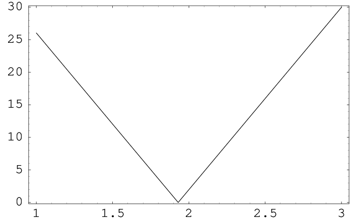
Refer to caption

bTb_{\rm T}

Figure E.1: Percentage difference between the numerical coefficients of ϵ1​ϵ2\epsilon_{1}\,\epsilon_{2} in PhP_{h} from WKB∗{\rm WKB*} and GFM{\rm GFM} as a function of bTb_{\rm T}. The difference vanishes for bT≃1.93b_{\rm T}\simeq 1.93 (≃2\simeq 2, the value used in the main text).
ϵ12\epsilon_{1}^{2}; PζP_{\zeta}, PhP_{h} ϵ22\epsilon_{2}^{2}; PζP_{\zeta} ϵ1​ϵ2\epsilon_{1}\,\epsilon_{2}; Pζ​(bS=2)P_{\zeta}(b_{\rm S}=2) ϵ1​ϵ2\epsilon_{1}\,\epsilon_{2}; Ph​(bT=2)P_{h}(b_{\rm T}=2)
WKB{\rm WKB} 2.3%2.3\% 3.0%3.0\% 353.3%353.3\% 37.2%37.2\%
WKB∗{\rm WKB*} 0.03%0.03\% 0.06%0.06\% 29.1%29.1\% 2.0%2.0\%
Table E.1: Percentage differences between the numerical coefficients of some second order terms in the power spectra given by WKB{\rm WKB} and WKB∗{\rm WKB*} with respect to those obtained by the GFM.
ϵ2​ϵ3\epsilon_{2}\,\epsilon_{3}; (dS=2)(d_{\rm S}=2) ϵ1​ϵ2\epsilon_{1}\,\epsilon_{2}; (bS−bT=0)(b_{\rm S}-b_{\rm T}=0) ϵ22\epsilon_{2}^{2}
WKB{\rm WKB} 56.7%56.7\% 1.5%1.5\% 117.3%117.3\%
WKB∗{\rm WKB*} 1.3%1.3\% 0.03%0.03\% 1.5%1.5\%
Table E.2: Percentage differences between the numerical coefficients of some second order terms in the scalar-to-tensor ratio given by WKB{\rm WKB} and WKB∗{\rm WKB*} with respect to those obtained from GFM. Note that the numerical coefficient of ϵ2​ϵ3\epsilon_{2}\,\epsilon_{3} in RR is the same as that in PζP_{\zeta}. Further, the coefficient of ϵ1​ϵ2\epsilon_{1}\,\epsilon_{2} does not depend on any undetermined parameters if bS=bTb_{\rm S}=b_{\rm T}.

Appendix F Perturbative approximations

In this Appendix we present a possible method of obtaining the complete result to second order in the HFF. We start by noting that any given function f=f⁡(x)=f⁡(ϵ,x)f=f(x)=f(\epsilon,x) can be written as the power series

f(ϵ,x)=∑n=0∞xnn!(−∑iϵ^i​ϵ^i+11−ϵ^1∂∂ϵ^i)nf(ϵ^i,x)≡∑n=0∞xnn!fn(x),\displaystyle f(\epsilon,x)=\sum_{n=0}^{\infty}\,\frac{x^{n}}{n!}\,\left(-\sum_{i}\,\frac{\hat{\epsilon}_{i}\,\hat{\epsilon}_{i+1}}{1-\hat{\epsilon}_{1}}\,\frac{\partial}{\partial\hat{\epsilon}_{i}}\right)^{n}f(\hat{\epsilon}_{i},x)\equiv\sum_{n=0}^{\infty}\,\frac{x^{n}}{n!}\,f_{n}(x)\ , (F.1)

where ϵ^i=ϵi​(x∗)\hat{\epsilon}_{i}=\epsilon_{i}(x_{*}) are the HFF evaluated at the horizon crossing (i.e. at x=x∗x=x_{*}) and f⁡(ϵ^i,x)=f⁡(ϵi=ϵ^i,x)f(\hat{\epsilon}_{i},x)=f(\epsilon_{i}=\hat{\epsilon}_{i},x). On using Eqs. (F.1) to express both ω2\omega^{2} and χ\chi in Eq. (4.6), we obtain

χ0​(x)​∑n=1∞xnn!​ωn2​(x)+[d2d​x2+∑m=0∞xmm!​ωm2​(x)]​∑n=1∞xnn!​χn​(x)=0,\displaystyle\chi_{0}(x)\,\sum_{n=1}^{\infty}\,\frac{x^{n}}{n!}\,\omega^{2}_{n}(x)+\left[\frac{{\mbox{${\rm d}$}}^{2}}{{\mbox{${\rm d}$}}x^{2}}+\sum_{m=0}^{\infty}\,\frac{x^{m}}{m!}\,\omega^{2}_{m}(x)\right]\,\sum_{n=1}^{\infty}\,\frac{x^{n}}{n!}\,\chi_{n}(x)=0\ , (F.2)

where we have used

[d2d​x2+ω02​(x)]​χ0​(x)=0,\displaystyle\left[\frac{{\mbox{${\rm d}$}}^{2}}{{\mbox{${\rm d}$}}x^{2}}+\omega^{2}_{0}(x)\right]\,\chi_{0}(x)=0\ , (F.3)

with ω02​(x)=ω2​(ϵi=ϵ^i,x)\omega^{2}_{0}(x)=\omega^{2}(\epsilon_{i}=\hat{\epsilon}_{i};x) and χ0​(x)\chi_{0}(x) is a linear combination (i.e. the MCE leading order solution) of Eq. (5.53) for Θ2​(x)=ω02​(x)\Theta^{2}(x)=\omega^{2}_{0}(x) and σ→x\sigma\to x in the argument of the Bessel functions. One may solve Eq. (F.2) for higher orders by introducing

xnn!​χn​(x)≡gn​(x)​χ0​(x),\displaystyle\frac{x^{n}}{n!}\,\chi_{n}(x)\equiv g_{n}(x)\,\chi_{0}(x)\ , (F.4)

and using the standard formulae for second order differential equations with a source term, so that

gn(x)=−∫∞xd​yχ02​(y)∫∞ydzχ02(z)[znn!ωn2(z)+∑m=1n−1gm(z)zn−mn−mωn−m2(z)].\displaystyle g_{n}(x)=-\int_{\infty}^{x}\,\frac{\mbox{${\rm d}$}y}{\chi^{2}_{0}(y)}\,\int_{\infty}^{y}\,\mbox{${\rm d}$}z\,\chi^{2}_{0}(z)\left[\frac{z^{n}}{n!}\,\omega^{2}_{n}(z)+\sum_{m=1}^{n-1}\,g_{m}(z)\,\frac{z^{n-m}}{n-m}\,\omega^{2}_{n-m}(z)\right]\ . (F.5)

The problem has therefore been reduced to computing 2​n2\,n integrals.

The above formalism can be modified in order to provide an alternative way for calculating the power spectra, spectral indices and runnings to second order in the HFF. We start from Eq. (5.1) using the exact relations

zT′′zT\displaystyle\frac{z^{\prime\prime}_{\rm T}}{z_{\rm T}} =\displaystyle= a2​H2​(2−ϵ1)\displaystyle a^{2}\,H^{2}\,\left(2-\epsilon_{1}\right)
zS′′zS\displaystyle\frac{z^{\prime\prime}_{\rm S}}{z_{\rm S}} =\displaystyle= a2​H2​(2−ϵ1+32​ϵ2−12​ϵ1​ϵ2+14​ϵ22+12​ϵ2​ϵ3).\displaystyle a^{2}\,H^{2}\,\left(2-\epsilon_{1}+\frac{3}{2}\,\epsilon_{2}-\frac{1}{2}\,\epsilon_{1}\,\epsilon_{2}+\frac{1}{4}\,\epsilon_{2}^{2}+\frac{1}{2}\,\epsilon_{2}\,\epsilon_{3}\right)\ .

With a redefinitions of the wave-function and variable

ψ=e−x/2μ,x~=ln(−kη)\displaystyle\psi={\rm e}^{-x/2}\,\mu\ ,\quad\quad\tilde{x}=\ln\left(-k\,\eta\right) (F.7)

we obtain

[d2d​x~2+ω~2​(x~)]​ψ​(x~)=0,\displaystyle\left[\frac{{\mbox{${\rm d}$}}^{2}}{{\mbox{${\rm d}$}}\tilde{x}^{2}}+\tilde{\omega}^{2}(\tilde{x})\right]\,\psi(\tilde{x})=0\ , (F.8)

where

ω~T2\displaystyle\tilde{\omega}^{2}_{\rm T} =\displaystyle= e2​x~−14−η2​a2​H2​(2−ϵ1)\displaystyle{\rm e}^{2\,\tilde{x}}-\frac{1}{4}-\eta^{2}a^{2}H^{2}\left(2-\epsilon_{1}\right)
ω~S2\displaystyle\tilde{\omega}^{2}_{\rm S} =\displaystyle= e2​x~−14−η2​a2​H2​(2−ϵ1+32​ϵ2−12​ϵ1​ϵ2+14​ϵ22+12​ϵ2​ϵ3).\displaystyle{\rm e}^{2\,\tilde{x}}-\frac{1}{4}-\eta^{2}a^{2}H^{2}\left(2-\epsilon_{1}+\frac{3}{2}\,\epsilon_{2}-\frac{1}{2}\,\epsilon_{1}\,\epsilon_{2}+\frac{1}{4}\,\epsilon_{2}^{2}+\frac{1}{2}\,\epsilon_{2}\,\epsilon_{3}\right)\ .

On now using the approximate relation

η≃−1a​H​(1+ϵ1+ϵ12+ϵ1​ϵ2),\displaystyle\eta\simeq-\frac{1}{a\,H}\,\left(1+\epsilon_{1}+\epsilon_{1}^{2}+\epsilon_{1}\,\epsilon_{2}\right)\ , (F.10)

the frequencies become

ω~T2\displaystyle\tilde{\omega}^{2}_{\rm T} ≃\displaystyle\simeq e2​x~−(94+3​ϵ1+4​ϵ12+4​ϵ1​ϵ2)\displaystyle{\rm e}^{2\,\tilde{x}}-\left(\frac{9}{4}+3\,\epsilon_{1}+4\,\epsilon_{1}^{2}+4\,\epsilon_{1}\epsilon_{2}\right)
ω~S2\displaystyle\tilde{\omega}^{2}_{\rm S} ≃\displaystyle\simeq e2​x~−(94+3​ϵ1+32​ϵ2+4​ϵ12+132​ϵ1​ϵ2+14​ϵ22+12​ϵ2​ϵ3),\displaystyle{\rm e}^{2\,\tilde{x}}-\left(\frac{9}{4}+3\,\epsilon_{1}+\frac{3}{2}\,\epsilon_{2}+4\,\epsilon_{1}^{2}+\frac{13}{2}\,\epsilon_{1}\epsilon_{2}+\frac{1}{4}\,\epsilon_{2}^{2}+\frac{1}{2}\,\epsilon_{2}\epsilon_{3}\right)\ ,

where we only keep the second order terms in the (still x~\tilde{x}-dependent) HFF. We can now expand linearly each HFF around the horizon crossing to obtain

d2​ψTd​x~2+[e2​x~−(94+3​ϵ^1+4​ϵ^12+4​ϵ^1​ϵ^2)]​ψT=−3​ϵ^1​ϵ^2​x~​ψT\displaystyle\frac{{\mbox{${\rm d}$}}^{2}\,\psi_{\rm T}}{{\mbox{${\rm d}$}}\,\tilde{x}^{2}}\!+\!\left[{\rm e}^{2\,\tilde{x}}\!-\!\left(\frac{9}{4}+3\,\hat{\epsilon}_{1}+4\,\hat{\epsilon}_{1}^{2}+4\,\hat{\epsilon}_{1}\hat{\epsilon}_{2}\right)\right]\!\psi_{\rm T}=-3\,\hat{\epsilon}_{1}\,\hat{\epsilon}_{2}\,\tilde{x}\,\psi_{\rm T}
(F.12)
d2​ψSd​x~2+[e2​x~−(94+3​ϵ^1+32​ϵ^2+4​ϵ^12+132​ϵ^1​ϵ^2+14​ϵ^22+12​ϵ^2​ϵ^3)]​ψS\displaystyle\frac{{\mbox{${\rm d}$}}^{2}\,\psi_{\rm S}}{{\mbox{${\rm d}$}}\,\tilde{x}^{2}}\!+\!\left[{\rm e}^{2\,\tilde{x}}\!-\!\left(\frac{9}{4}+3\,\hat{\epsilon}_{1}+\frac{3}{2}\,\hat{\epsilon}_{2}+4\,\hat{\epsilon}_{1}^{2}+\frac{13}{2}\,\hat{\epsilon}_{1}\hat{\epsilon}_{2}+\frac{1}{4}\,\hat{\epsilon}_{2}^{2}+\frac{1}{2}\,\hat{\epsilon}_{2}\hat{\epsilon}_{3}\right)\right]\!\psi_{\rm S}
=−3​(ϵ^1​ϵ^2+12​ϵ^2​ϵ^3)​x~​ψS,\displaystyle\quad\quad\quad\quad=-3\left(\hat{\epsilon}_{1}\,\hat{\epsilon}_{2}+\frac{1}{2}\,\hat{\epsilon}_{2}\,\hat{\epsilon}_{3}\right)\tilde{x}\,\psi_{\rm S}\ ,

which, beside the use of x~\tilde{x} instead of xx and the appearance of ω~\tilde{\omega} instead of ω\omega, is equivalent to the expansion in Eq. (F.1) for f=ω~2f=\tilde{\omega}^{2} and can be solved by means of a standard perturbative approach (such as in Ref. [75]). The method is close to GFM and gives the same results of Eq. (41) in Ref. [75] and Eq. (29) in Ref. [68] for the scalar and tensor power spectra, respectively.

Let us finally note that, for the GFM, the scalar spectral index and its running are calculated by taking the derivative of Eq. (41) in Ref. [75], i.e. the power spectra evaluated at k=a​Hk=a\,H, in terms of ln⁡k\ln k, while in our MCE (but also in the WKB approximation [70, 71]) the dependences in ln⁡(k/k∗)\ln\left(k/k_{*}\right) are obtained explicitly (see, for example, Eqs. (6.37a) and (6.37b)).

Appendix G MCE and Black Holes

In this Appendix we employ the Method of Comparison Equations to study the propagation of a massless minimally coupled scalar field on the Schwarzschild background as an example of a potential with two turning point in the wave equation. In particular, we show that this method allows us to obtain explicit approximate expressions for the radial modes with energy below the peak of the effective potential which are fairly accurate over the whole region outside the horizon. This case can be of particular interesting, for example, for the problem of black hole evaporation.

Wave equations on black hole backgrounds cannot be solved exactly in terms of known simple functions (for a review, see, e.g., Ref. [83]). Although it is usually fairly easy to find asymptotic expressions near the (outer) horizon or at spatial infinity, numerical analysis is what one eventually employs to obtain a detailed profile of the wave-functions. However, our understanding of the field dynamics on curved backgrounds would still benefit of analytical approximations to the exact modes, for example in the study of the (renormalized) energy-momentum tensor of quantum fields [33] and, in particular, of the Hawking radiation [84, 85], or of quasi-normal modes [86].

By making use of the black hole symmetry, one can usually separate the wave-functions and reduce the problem to the one task of solving a second order differential equation for the radial part. The latter takes the form of the one-dimensional Schrödinger equation for the transmission through a potential barrier [83]

[d2d​x2+Qs​(x)]​ψ=0,\displaystyle\left[\frac{\mbox{${\rm d}$}^{2}}{\mbox{${\rm d}$}x^{2}}+Q_{s}(x)\right]\psi=0\ , (G.1)

and, for the general case of a Kerr-Newman black hole, is known as the Teukolsky master equation for waves of spin-weight s=0s=0, 11 and 22 [87, 83].

In the next Section, we shall briefly review the equation of motion for massless scalar fields on a spherically symmetric black hole background. This includes the simplest case of linear perturbations of a Schwarzschild black hole which will be used to show the application of our method in all details (including the use of a convenient radial coordinate and rescaling of the wave-function). In Section G.2, we shall then apply the MCE and obtain approximate expressions for scalar wave-modes with energy below the peak of the potential. This case is of particular interest, for example, for evaluating the grey-body factors involved in the Hawking effect [84, 85]. It also presents a major complication with respect to the typical case of Cosmological Pertubations, namely the presence of two zeros of the potential (“turning points”). We shall use units with c=G=1c=G=1. The last three Sections will give some tecnical results which complete this Appendix.

G.1 Scalar field on Schwarzschild background

Let us begin by recalling that the metric in a static and spherically symmetric vacuum space-time can be written in general as

d​s2=h⁡(r)​d​t2−d​r2h⁡(r)−r2​d​Ω2,\displaystyle\mbox{${\rm d}$}s^{2}=h(r)\,\mbox{${\rm d}$}t^{2}-\frac{\mbox{${\rm d}$}r^{2}}{h(r)}-r^{2}\,\mbox{${\rm d}$}\Omega^{2}\ , (G.2)

where d​Ω\mbox{${\rm d}$}\Omega is the area element on the unit two-sphere. The propagation of massless, minimally coupled scalar particles in this background is governed by the Klein-Gordon equation Φ;μ;μ=0\Phi^{;\mu}_{\ \ ;\mu}=0. Due to the symmetry of the background, the field Φ\Phi can be decomposed into eigenmodes of normal frequency ω¯\bar{\omega} and angular momentum numbers ℓ\ell, mm as [83]

Φ⁡(t,r,Ω)=e−i​ω¯​t​Yℓm​(Ω)​R​(r),\displaystyle\Phi(t,r,\Omega)={\rm e}^{-i\,\bar{\omega}\,t}\,Y^{m}_{\ell}(\Omega)\,R(r)\ , (G.3)

where YℓmY_{\ell}^{m} are spherical harmonics. The Klein-Gordon equation then separates and the dynamics is described by the function RR which satisfies the radial equation

dd​r​[r2​h​(r)​d​R​(r)d​r]+[ω¯2​r2h⁡(r)−ℓ⁡(ℓ+1)]​R​(r)=0,\displaystyle\frac{\mbox{${\rm d}$}}{\mbox{${\rm d}$}r}\left[r^{2}\,h(r)\,\frac{\mbox{${\rm d}$}R(r)}{\mbox{${\rm d}$}r}\right]+\left[\frac{\bar{\omega}^{2}\,r^{2}}{h(r)}-\ell\,(\ell+1)\right]R(r)=0\ , (G.4)

where ℓ⁡(ℓ+1)\ell\,(\ell+1) is the separation constant. No exact solution of the above equation is known even for as simple a background as the four-dimensional Schwarzschild space-time with

h⁡(r)=1−r~−1,\displaystyle h(r)=1-\tilde{r}^{-1}\ , (G.5)

where we have introduced the dimensionless radial coordinate r~=r/rH\tilde{r}=r/r_{\rm H} and rHr_{\rm H} is the Schwarzschild radius.

It is now convenient to introduce the ‘‘tortoise-like’’ coordinate 11 1 A similar coordinate was already used in Ref. [88].

d​x=d​r~r~​h​(r~),\displaystyle\mbox{${\rm d}$}\,x=\frac{\mbox{${\rm d}$}\,\tilde{r}}{\tilde{r}\,h(\tilde{r})}\ , (G.6a)
and the new radial function
R[r~(x)]=exp[−12∫xh(x′)dx′]χ[r~(x)],\displaystyle R\left[\tilde{r}(x)\right]={\rm exp}\left[-\frac{1}{2}\,\int^{x}\,h(x^{\prime})\,\mbox{${\rm d}$}\,x^{\prime}\right]\chi\left[\tilde{r}(x)\right]\ , (G.6b)

so that the radial equation takes the Schrödinger form

d2​χ​(x)d​x2+{ω~2​r~2​(x)−ℓ⁡(ℓ+1)​h​[r~​(x)]−14​h2​[r~​(x)]−12​d​h​[r~​(x)]d​x}​χ​(x)=0.\displaystyle\frac{\mbox{${\rm d}$}^{2}\,\chi(x)}{\mbox{${\rm d}$}x^{2}}+\left\{\tilde{\omega}^{2}\,\tilde{r}^{2}(x)-\ell\,(\ell+1)\,h[\tilde{r}(x)]-\frac{1}{4}\,h^{2}[\tilde{r}(x)]-\frac{1}{2}\,\frac{\mbox{${\rm d}$}h[\tilde{r}(x)]}{\mbox{${\rm d}$}x}\right\}\chi(x)=0\ . (G.7)

where we also defined the dimensionless energy ω~≡ω¯​rH\tilde{\omega}\equiv\bar{\omega}\,r_{\rm H}. For the four-dimensional Schwarzschild case we have

x⁡(r~)=ln⁡(r~−1),\displaystyle x(\tilde{r})=\ln(\tilde{r}-1)\ , (G.8)

so that the new variable xx ranges from x⁡(r~H=1)=−∞x(\tilde{r}_{\rm H}=1)=-\infty to x⁡(r~=+∞)=+∞x(\tilde{r}=+\infty)=+\infty and xx and χ⁡(x)\chi(x) are of Langer’s form [37]. The Klein-Gordon equation finally becomes

[d2d​x2+ω2​(x)]​χ​(x)=0,\displaystyle\left[\frac{{\mbox{${\rm d}$}}^{2}}{{\mbox{${\rm d}$}}x^{2}}+\omega^{2}(x)\right]\,\chi(x)=0\ , (G.9)

where the “frequency”

ω2​(x)=ω~2​(1+ex)2−ℓ⁡(ℓ+1)​ex1+ex−ex​(2+ex)4​(1+ex)2,\displaystyle\omega^{2}(x)=\tilde{\omega}^{2}\left(1+{\rm e}^{x}\right)^{2}-\frac{\ell\,(\ell+1)\,{\rm e}^{x}}{1+{\rm e}^{x}}-\frac{{\rm e}^{x}\left(2+{\rm e}^{x}\right)}{4\,\left(1+{\rm e}^{x}\right)^{2}}\ , (G.10)

is not necessarily a positive quantity. In fact, the above expression shows two qualitatively different behaviors depending on the values of ω~\tilde{\omega} and ℓ\ell. In particular, for a given angular momentum ℓ\ell, there exists a critical value

ω~c=ω~c​(ℓ),\displaystyle\tilde{\omega}_{\rm c}=\tilde{\omega}_{\rm c}(\ell)\ , (G.11)

such that if the energy ω~>ω~c\tilde{\omega}>\tilde{\omega}_{\rm c} there are no turning points, otherwise there are two, say ω⁡(x1)=ω⁡(x2)=0\omega(x_{1})=\omega(x_{2})=0 with x1<x2x_{1}<x_{2}. The latter case is the one we want to analyze in detail (see Sec. G.2.1 for more details and the solid line in Fig. G.1 for an example).

G.2 MCE solutions

Referring to Section 4.4 for the basic formulae characterising the MCE, we can find the approximate solution of Eq. (G.9),

χMCE(x)=(d​σd​x)−1/2U(σ),\displaystyle\chi_{\rm MCE}(x)=\left(\frac{{\mbox{${\rm d}$}}\sigma}{{\mbox{${\rm d}$}}x}\right)^{-1/2}U(\sigma)\ , (G.12)

which is valid in the whole range of xx and including the turning points.

We are now dealing with a problem of the form (G.9) with two turning points, x1<x2x_{1}<x_{2}. In order to implement the MCE, we need a “comparison frequency” with the same behavior. We shall use the Morse potential [89]

Θ2​(σ)=A​e2​σ−B​eσ+D.\displaystyle\Theta^{2}(\sigma)=A\,{\rm e}^{2\,\sigma}-B\,{\rm e}^{\sigma}+D\ . (G.13)

The coefficients AA and BB are then fixed by imposing that the turning points of the comparison function are the same as those of the exact frequency, that is

Θ⁡(σ1=x1)=Θ⁡(σ2=x2)=0,\displaystyle\Theta(\sigma_{1}=x_{1})=\Theta(\sigma_{2}=x_{2})=0\ , (G.14a)
and the coefficient DD will then follow form the relation
ξ≡∫x1x2−ω2​(y)​𝑑y=∫x1x2−Θ2​(ρ)​𝑑ρ.\displaystyle\xi\equiv\int_{x_{1}}^{x_{2}}\sqrt{-\,\omega^{2}(y)}\,{\mbox{${\rm d}$}}\,y=\int_{x_{1}}^{x_{2}}\sqrt{-\,\Theta^{2}(\rho)}\,{\mbox{${\rm d}$}}\,\rho\ . (G.14b)

The system of non-linear equations (G.14a) and (G.14b) thus yields

A\displaystyle A =\displaystyle\!=\! 4​ξ2π2​(w1+w2−2​w1​w2)2\displaystyle\frac{4\,\xi^{2}}{\pi^{2}\left({w_{1}+w_{2}}-2\,\sqrt{w_{1}\,w_{2}}\right)^{2}} (G.15a)
B\displaystyle B =\displaystyle\!=\! (w1+w2)​A\displaystyle\left(w_{1}+w_{2}\right)A (G.15b)
D\displaystyle D =\displaystyle\!=\! w1​w2​A,\displaystyle w_{1}\,w_{2}\,A\ , (G.15c)

where the exact expression for ξ\xi is given in Sec. G.2.2. A sample plot of both the exact frequency and the comparison function thus obtained is given in Fig. G.1.

Refer to caption

xx

Figure G.1: Comparison between the exact potential −ω2​(x)-\omega^{2}(x) (solid line) and the approximate Morse potential −Θ2​[σ​(x)]-\Theta^{2}[\sigma(x)] obtained after solving Eqs. (G.14a) and (G.14b) (dotted line) for ω~=1/2\tilde{\omega}=1/2 and ℓ=2\ell=2. The two turning points are x1≈−3.13x_{1}\approx-3.13 and x2≈1.23x_{2}\approx 1.23.

The “comparison solution” is a linear combination of confluent hypergeometric functions [39] of the type F11{}_{1}{\rm F}_{1} (for more details, see Ref. [89]),

U⁡(σ)\displaystyle U(\sigma) =\displaystyle\!=\! C+​ei⁡(A​eσ+D​σ)​F11​(12+i​D+i​B2​A,1+2​i​D,−2​i​A​eσ)\displaystyle C_{+}\,{\rm e}^{i\,\left(\sqrt{A}\,{\rm e}^{\sigma}+\sqrt{D}\,\sigma\right)}\,{}_{1}{\rm F}_{1}\left(\frac{1}{2}+i\,\sqrt{D}+i\,\frac{B}{2\,\sqrt{A}},1+2\,i\,\sqrt{D},-2\,i\,\sqrt{A}\,{\rm e}^{\sigma}\right) (G.16)
+C−​ei⁡(A​eσ−D​σ)​F11​(12−i​D+i​B2​A,1−2​i​D,−2​i​A​eσ),\displaystyle\!\!\!\!\!\!\!\!\!\!\!\!\!\!\!\!\!\!\!\!+C_{-}\,{\rm e}^{i\,\left(\sqrt{A}\,{\rm e}^{\sigma}-\sqrt{D}\,\sigma\right)}\,{}_{1}{\rm F}_{1}\left(\frac{1}{2}-i\,\sqrt{D}+i\,\frac{B}{2\,\sqrt{A}},1-2\,i\,\sqrt{D},-2\,i\,\sqrt{A}\,{\rm e}^{\sigma}\right)\ ,

and σ⁡(x)\sigma(x) is given implicitly by Eq. (4.31) with

∫x1σΘ2​(ρ)​𝑑ρ=Θ2​(σ)\displaystyle\int_{x_{1}}^{\sigma}\sqrt{\Theta^{2}(\rho)}\,{\mbox{${\rm d}$}}\,\rho=\sqrt{\Theta^{2}(\sigma)} (G.17)
−ln⁡[(2​A​eσ−B+2​A​Θ2​(σ))B2​A​(2​D​e−σ−B+2​e−σ​D​Θ2​(σ))D].\displaystyle-\ln\left[\left(2\,A\,{\rm e}^{\sigma}-B+2\,\sqrt{A\,\Theta^{2}(\sigma)}\right)^{\frac{B}{2\,\sqrt{A}}}\left(2\,D\,{\rm e}^{-\sigma}-B+2\,{\rm e}^{-\sigma}\,\sqrt{\,D\,\Theta^{2}(\sigma)}\right)^{\sqrt{D}}\right]\ .

The above expression is rather complex. Hence, we just consider the asymptotic relation between σ\sigma and xx to the left of the smaller turning point (that is, for x≪x1x\ll x_{1})

σ⁡(x)≃ω~D​x\displaystyle\sigma(x)\simeq\frac{\tilde{\omega}}{\sqrt{D}}\,x (G.18a)
and to the right of the larger one (x≫x2x\gg x_{2})
A​eσ⁡(x)−B2​A​σ​(x)≃ω~​(ex+x).\displaystyle\sqrt{A}\,{\rm e}^{\sigma(x)}-\frac{B}{2\,\sqrt{A}}\,\sigma(x)\simeq\tilde{\omega}\left({\rm e}^{x}+x\right)\ . (G.18b)

As an approximate expression for σ⁡(x)\sigma(x) for x<κ1​x1x<\kappa_{1}\,x_{1} (with κ1≳1\kappa_{1}\gtrsim 1) we shall then use Eq. (G.18a) and the condition that σ⁡(x1)=x1\sigma(x_{1})=x_{1}. Analogously, for x>κ2​x2x>\kappa_{2}\,x_{2} (with κ2≳1\kappa_{2}\gtrsim 1) we shall use the approximate solution of Eq. (G.18b) to next-to-leading order for large xx. Moreover, in the region between κ1​x1\kappa_{1}\,x_{1} and κ2​x2\kappa_{2}\,x_{2} we shall use an interpolating cubic function. The reason for introducing two new parameters κ1\kappa_{1} and κ2≳1\kappa_{2}\gtrsim 1 is that the asymptotic forms in Eqs. (G.18a) and (G.18b) may differ significantly from the correct σ⁡(x)\sigma(x) around the turning points x1x_{1} and x2x_{2} and suitable values of κ1\kappa_{1} and κ2\kappa_{2} usually improve the final result. To summarize, we have

σ={ω~D​x+x1​(1−ω~D),x0<x<κ1​x1C0+C1​x+C2​x2+C3​x3,κ1​x1<x<κ2​x2x+ln⁡(ω~A),x>κ2​x2,\displaystyle\sigma\!=\!\left\{\begin{array}[]{ll}\displaystyle\frac{\tilde{\omega}}{\sqrt{D}}\,x+x_{1}\left(1-\frac{\tilde{\omega}}{\sqrt{D}}\right)\ ,&x_{0}<x<\kappa_{1}x_{1}\\ \\ C_{0}+C_{1}\,x+C_{2}\,x^{2}+C_{3}\,x^{3},&\kappa_{1}x_{1}<x<\kappa_{2}x_{2}\\ \\ x+\ln\left(\displaystyle\frac{\tilde{\omega}}{\sqrt{A}}\right)\ ,&x>\kappa_{2}x_{2}\ ,\end{array}\right.

with κ1\kappa_{1} and κ2≳1\kappa_{2}\gtrsim 1 and x0<κ1​x1x_{0}<\kappa_{1}\,x_{1} is the value of xx at which we wish to impose the initial conditions for χ⁡(x)\chi(x) and its derivative 22 2 Of course, if we are interested in setting the initial conditions at x0≫x2x_{0}\gg x_{2} the expressions must be adjusted correspondingly.. The explicit expressions for the coefficients C0C_{0}, C1C_{1}, C2C_{2} and C3C_{3} are rather cumbersome and will be given in Sec. G.2.3.

σ\sigma Refer to caption χ\chi Refer to caption xx                           xx

Refer to caption
Refer to caption
Refer to caption

        (a)               (b)               (c)

Figure G.2: Upper left graph: The function σ=σ⁡(x)\sigma=\sigma(x) obtained by integrating Eq. (4.31) numerically (solid line) and its approximate expression (G.2) with κ1=1\kappa_{1}=1 and κ2=3\kappa_{2}=3 (dashed line). Upper right graph: Comparison between the exact solution (solid line) and the approximate MCE solution (G.12) with σ⁡(x)\sigma(x) evaluated numerically (dashed line) for C+≈0.517−0.228​iC_{+}\approx 0.517-0.228\,i and C−≈0.517+0.228​iC_{-}\approx 0.517+0.228\,i. Panel (a) shows the percentage error for the same approximate function σ\sigma given in the upper left graph. Panel (b) shows the percentage error for the approximate χ\chi in the upper right graph for x<x1x<x_{1} and panel (c) for x2<xx_{2}<x. All plots are for ω~=1/2\tilde{\omega}=1/2, ℓ=2\ell=2 as in Fig. G.1.

In the upper left panel of Fig. G.2, we plot σ⁡(x)\sigma(x) for the same values of ω~\tilde{\omega} and ℓ\ell used in Fig. G.1. The solid line represents the numerical solution of Eq. (4.31) and the dashed line the approximate expression (G.2) with κ1=1\kappa_{1}=1 and κ2=3\kappa_{2}=3. It is clear that these values of κ1\kappa_{1} and κ2\kappa_{2} already lead to a very good approximation for σ\sigma around the turning points x1x_{1} and x2x_{2} and that larger values of κ1\kappa_{1} or κ2\kappa_{2} would not improve significantly the final result. In the upper right panel of Fig. G.2, we compare an MCE approximate wave-function with the exact solution (solid line) obtained numerically for the same case. The MCE solution shown by a dashed line is given by the expression (G.12) with U⁡(σ)U(\sigma) as in Eq. (G.16) and σ⁡(x)\sigma(x) determined by solving Eq. (4.31) numerically. The coefficients C±C_{\pm} are fixed by imposing that the MCE mode and its derivative equal the corresponding values of the chosen numerical solution at x=−20x=-20. Since the two curves coincide almost everywhere, it is clear that solving the approximate equation (4.31) for σ⁡(x)\sigma(x) is, to all practical extents, equivalent to solving the original equation (G.9).

In order to further clarify this point, in panel (a) of Fig. G.2, we plot the relative difference (in percent) between the approximate expression (G.2) and the exact numerical solution of Eq. (4.31). We can see that the error is less than 10%10\% almost everywhere, except near the zero of σ⁡(x)\sigma(x). In the same figure, we also show the percentage error for the approximate solution shown in Fig. G.2 on the left of x1x_{1} and on the right of x2x_{2}. The latter error remains small, too, except around the zeros of χ\chi due to the slight difference in phases.

Refer to caption
Refer to caption
Refer to caption

        (a)              (b)               (c)

Figure G.3: Comparison between the exact solution (solid line) and the approximate MCE solution (G.12) with σ⁡(x)\sigma(x) given in Eq. (G.2) with κ1=1\kappa_{1}=1 and κ2=3\kappa_{2}=3 (dashed line) for ω~=1/2\tilde{\omega}=1/2 and ℓ=2\ell=2 (same as in Figs. G.1 and G.2). Panel (a) shows the result for x<κ1​x1x<\kappa_{1}\,x_{1}, panel (b) for κ1​x1<x<κ2​x2\kappa_{1}\,x_{1}<x<\kappa_{2}\,x_{2} and panel (c) for x>κ2​x2x>\kappa_{2}\,x_{2}.

Finally, in Fig. G.3, the dashed lines represent the same MCE solution with σ⁡(x)\sigma(x) given by its analytical approximation in Eq. (G.2) with κ1=1\kappa_{1}=1 and κ2=3\kappa_{2}=3. This is the fully analytical expression obtained from the application of the MCE and is still remarkably good, with a more significant error around the larger turning point (x2≈1.23x_{2}\approx 1.23). From the three graphs in Fig. G.3 and the upper left panel in Fig. G.2, it clearly appears that such an error develops in the region between the two turning points, where the discrepancy between the exact σ⁡(x)\sigma(x) and the approximate expression (G.2) is indeed larger. In this respect, let us note that, had we imposed initial conditions at x≫x2x\gg x_{2}, the larger error would have occurred around the smaller turning point (x1≈−3.13x_{1}\approx-3.13). Moreover, when we used a linear (or quadratic) interpolating function for κ1​x1<x<κ2​x2\kappa_{1}\,x_{1}<x<\kappa_{2}\,x_{2}, the accuracy was (expectedly) worse. Should one need better accuracy, a higher order polynomial interpolation between κ1​x1\kappa_{1}\,x_{1} and κ2​x2\kappa_{2}\,x_{2} could therefore be used instead.

Let us now make a few remarks. Firstly, the application of the MCE is not as straightforward as the standard WKB approximation. In fact, the MCE usually requires solving some technical tasks specific to the problem at hand in order to obtain the argument σ=σ⁡(x)\sigma=\sigma(x) of the known function U=U⁡(σ)U=U(\sigma). In the present case, with two turning points, all expressions become more involved. The best approximation for σ⁡(x)\sigma(x) we found convenient to display in Eq. (G.2) makes use of a cubic interpolation over the region containing the two turning points and is given in terms of two arbitrary parameters κ1\kappa_{1} and κ2\kappa_{2} which can be fixed in order to minimize the error. Of course, one could employ higher order interpolating functions and further improve the result at the price of complexity if better accuracy is needed. Our aim for the work presented in this Appendix was mainly to test the effectiveness of the MCE to produce approximate wave modes on black hole backgrounds.

In the next three technical Sections we give explicit expressions for the turning points, the calculation of the quantity ξ\xi and some details of the cubic interpolation used to obtain σ⁡(x)\sigma(x).

G.2.1 Turning Points

If we define w=exw={\rm e}^{x}, we see that ω2​(x)=0\omega^{2}(x)=0 for the exact frequency in Eq. (G.10) becomes the quartic polynomial equation

w4+4​w3+b​w2+c​w+1=0,\displaystyle w^{4}+4\,w^{3}+b\,w^{2}+c\,w+1=0\ , (G.25a)
with
b\displaystyle b =\displaystyle\!=\! 6−14​ω~2−ℓ⁡(ℓ+1)ω~2\displaystyle 6-\frac{1}{4\,{\tilde{\omega}}^{2}}-\frac{\ell\left(\ell+1\right)}{{\tilde{\omega}}^{2}} (G.25b)
c\displaystyle c =\displaystyle\!=\! 4−12​ω~2−ℓ⁡(ℓ+1)ω~2.\displaystyle 4-\frac{1}{2\,{\tilde{\omega}}^{2}}-\frac{\ell\left(\ell+1\right)}{{\tilde{\omega}}^{2}}\ . (G.25c)

Its four roots can be written as

wi=−1+ϵi2​4−23​b+γ3−θi2​8−43​b+ϵi​4​b−16−2​c4−23​b+γ3−γ3,\displaystyle w_{i}=-1+\frac{\epsilon_{i}}{2}\sqrt{4-\frac{2}{3}\,b+\frac{\gamma}{3}}-\frac{\theta_{i}}{2}\sqrt{8-\frac{4}{3}\,b+\epsilon_{i}\frac{4\,b-16-2\,c}{{\sqrt{4-\frac{2}{3}\,b+\frac{\gamma}{3}}}}-\frac{\gamma}{3}}\ , (G.26a)
where i=1,…,4i=1,\ldots,4 and
α\displaystyle\!\!\!\!\!\!\!\!\!\!\!\!\!\!\!\!\alpha =\displaystyle\!=\! 12+b2−12​c\displaystyle 12+b^{2}-12\,c (G.26b)
β\displaystyle\!\!\!\!\!\!\!\!\!\!\!\!\!\!\!\!\beta =\displaystyle\!=\! 2​b3−36​b​c+27​c2+432−72​b\displaystyle 2\,b^{3}-36\,b\,c+27\,c^{2}+432-72\,b (G.26c)
γ\displaystyle\!\!\!\!\!\!\!\!\!\!\!\!\!\!\!\!\gamma =\displaystyle\!=\! 213​α(β+β2−4​α3)13+(β+β2−4​α3)13213.\displaystyle\frac{2^{\frac{1}{3}}\,\alpha}{\left(\beta+\sqrt{\beta^{2}-4\,\alpha^{3}}\right)^{\frac{1}{3}}}+\frac{\left(\beta+\sqrt{\beta^{2}-4\,\alpha^{3}}\right)^{\frac{1}{3}}}{2^{\frac{1}{3}}}\ . (G.26d)

The coefficients ϵ1=ϵ2=−ϵ3=−ϵ4=θ1=−θ2=θ3=−θ4=1\epsilon_{1}=\epsilon_{2}=-\epsilon_{3}=-\epsilon_{4}=\theta_{1}=-\theta_{2}=\theta_{3}=-\theta_{4}=1, and the values of ω~\tilde{\omega} and ℓ\ell determine the signs of the roots. There can be at most two positive roots, in which case, say, w3≤w4≤0≤w1=ex1≤w2=ex2w_{3}\leq w_{4}\leq 0\leq w_{1}={\rm e}^{x_{1}}\leq w_{2}={\rm e}^{x_{2}}, and only x1x_{1} and x2x_{2} can be valid turning points. The critical value of ω~\tilde{\omega} in Eq. (G.11) is then determined by the condition 0≤w1=w20\leq w_{1}=w_{2}.

G.2.2 Evaluation of ξ\xi

In order to evaluate the integral in Eq. (G.14b), we start from the general relation (again with w=exw={\rm e}^{x})

1ω~​∫x1ln⁡(w)−ω2​(y)​𝑑y=(w−w3)​(w−w1)​(w−w2)w−w4+1(w1−w3)​(w4−w2)\displaystyle\frac{1}{\tilde{\omega}}\int_{x_{1}}^{\ln(w)}\sqrt{-\,\omega^{2}(y)}\,{\mbox{${\rm d}$}}\,y=\sqrt{\frac{(w-w_{3})(w-w_{1})(w-w_{2})}{w-w_{4}}}+\frac{1}{\sqrt{(w_{1}-w_{3})(w_{4}-w_{2})}}
×{(w3−w1)(w4−w2)E(z;W)−(w4−w1)(w4−w2)F(z;W)\displaystyle\quad\quad\times\left\{(w_{3}-w_{1})(w_{4}-w_{2})\,{\rm E}(z;W)-(w_{4}-w_{1})(w_{4}-w_{2})\,{\rm F}(z;W)\phantom{\frac{A}{B}}\right.
+(w4−w1)​(w3+w4+w1+w2+2)​Π​[w1−w2w4−w2;z;W]\displaystyle\quad\quad\phantom{\times\ \ }\left.+(w_{4}-w_{1})(w_{3}+w_{4}+w_{1}+w_{2}+2)\,{\rm\Pi}\!\left[\frac{w_{1}-w_{2}}{w_{4}-w_{2}};z;W\right]\right.
−2​(w4−w1)​(w3+1)​(w2+1)​Π​[(w4+1)​(w1−w2)(w1+1)​(w4−w2);z;W]\displaystyle\quad\quad\phantom{\times\ \ }\left.-2\,(w_{4}-w_{1})(w_{3}+1)(w_{2}+1)\,{\rm\Pi}\!\left[\frac{(w_{4}+1)(w_{1}-w_{2})}{(w_{1}+1)(w_{4}-w_{2})};z;W\right]\right.
+2(w4−w1)w3w2Π[w4​(w1−w2)w1​(w4−w2);z;W]},\displaystyle\quad\quad\phantom{\times\ \ }\left.+2\,(w_{4}-w_{1})w_{3}\,w_{2}\,{\rm\Pi}\!\left[\frac{w_{4}\,(w_{1}-w_{2})}{w_{1}\,(w_{4}-w_{2})};z;W\right]\right\}\ , (G.27)

where E, F and Π{\rm\Pi} are elliptic functions [39],

z=ArcSin⁡[(w−w1)​(w4−w2)(w−w4)​(w1−w2)],\displaystyle z={\rm ArcSin}\!\left[\sqrt{\frac{(w-w_{1})(w_{4}-w_{2})}{(w-w_{4})(w_{1}-w_{2})}}\right]\ , (G.28)
W=(w3−w4)​(w1−w2)(w3−w1)​(w4−w2),\displaystyle W=\frac{(w_{3}-w_{4})(w_{1}-w_{2})}{(w_{3}-w_{1})(w_{4}-w_{2})}\ , (G.29)

and wi=exiw_{i}={\rm e}^{x_{i}} are the roots of ω2​(x)\omega^{2}(x) as given in the previous Section. The above expression evaluated at w=w2w=w_{2} yields

ξ=ω~(w1−w3)​(w4−w2){(w3−w1)(w4−w3)E(W)+(w4−w1)(w2−w4)K(W)\displaystyle\xi=\frac{\tilde{\omega}}{\sqrt{(w_{1}-w_{3})(w_{4}-w_{2})}}\left\{(w_{3}-w_{1})(w_{4}-w_{3})\,{\rm E}(W)+(w_{4}-w_{1})\,(w_{2}-w_{4})\,{\rm K}(W)\right.
+(w4−w1)​(w3+w4+w1+w2+2)​Π​[w1−w2w4−w2;W]\displaystyle\left.+(w_{4}-w_{1})\,(w_{3}+w_{4}+w_{1}+w_{2}+2)\,{\rm\Pi}\!\left[\frac{w_{1}-w_{2}}{w_{4}-w_{2}};W\right]\right.
−2​(w3+1)​(w2+1)​(w4−w1)​Π​[(w4+1)​(w1−w2)(w1+1)​(w4−w2);W]\displaystyle\left.-2(w_{3}+1)(w_{2}+1)(w_{4}-w_{1})\,{\rm\Pi}\!\left[\frac{(w_{4}+1)(w_{1}-w_{2})}{(w_{1}+1)(w_{4}-w_{2})};\!W\!\right]\right.
+2w3w2(w4−w1)Π[w4​(w1−w2)w1​(w4−w2);W]},\displaystyle\phantom{\times\ \ }\left.+2\,w_{3}\,w_{2}\,(w_{4}-w_{1})\,{\rm\Pi}\!\left[\frac{w_{4}\,(w_{1}-w_{2})}{w_{1}\,(w_{4}-w_{2})};W\right]\right\}\ , (G.30)

in which we used E(π/2,q)=(\pi/2;q)=E(q)(q), F(π/2,q)=(\pi/2;q)=K(q)(q) and Π⁡(p,π/2,q)=Π⁡(p,q)\Pi(p;\pi/2;q)=\Pi(p,q) [39].

G.2.3 Cubic interpolation

In Section G.2, we use the analytic approximation for σ⁡(x)\sigma(x) in Eq. (G.2) which involves the cubic interpolation

σ=C0+C1​x+C2​x2+C3​x3,\displaystyle\sigma=C_{0}+C_{1}\,x+C_{2}\,x^{2}+C_{3}\,x^{3}\ , (G.31)

for κ1​x1<x<κ2​x2\kappa_{1}\,x_{1}<x<\kappa_{2}\,x_{2}. The above coefficients CiC_{i}, with i=0,…,3i=0,\ldots,3, can be easily expressed in terms of the parameters AA, BB and DD for the Morse potential (G.13) as

C0=κ1​x1​(2​D−1)​κ22​x22​(κ2​x2−κ1​x1)−2​D​ln⁡(2​A)​κ1​x1​(3​κ2​x2−κ1​x1)2​D​(κ2​x2−κ1​x1)3\displaystyle C_{0}={\kappa_{1}}\,{x_{1}}\,\frac{\left(2\,{\sqrt{D}-1}\right)\,{{\kappa_{2}}}^{2}\,{{x_{2}}}^{2}\,\left({\kappa_{2}}\,{x_{2}}-{\kappa_{1}}\,{x_{1}}\right)-2\,{\sqrt{D}}\,\ln\left(2\,{\sqrt{A}}\right){\kappa_{1}}\,{x_{1}}\left(3\,{\kappa_{2}}\,{x_{2}}-{\kappa_{1}}\,{x_{1}}\right)}{2\,{\sqrt{D}}\,{\left({\kappa_{2}}\,{x_{2}}-{\kappa_{1}}\,{x_{1}}\right)}^{3}}
C1=(κ2​x2−κ1​x1)​[κ2​x2​(2​κ1​x1+κ2​x2)−2​D​κ1​x1​(4​κ2​x2−κ1​x1)]2​D​(κ2​x2−κ1​x1)3\displaystyle C_{1}=\frac{\left({\kappa_{2}}\,{x_{2}}-{\kappa_{1}}\,{x_{1}}\right)\left[{\kappa_{2}}\,{x_{2}}\,\left(2\,{\kappa_{1}}\,{x_{1}}+{\kappa_{2}}\,{x_{2}}\right)-2\,{\sqrt{D}}\,{\kappa_{1}}\,{x_{1}}\,\left(4\,{\kappa_{2}}\,{x_{2}}-{\kappa_{1}}\,{x_{1}}\right)\right]}{2\,{\sqrt{D}}\,{\left({\kappa_{2}}\,{x_{2}}-{\kappa_{1}}\,{x_{1}}\right)}^{3}}
+12​D​ln⁡(2​A)​κ1​κ2​x1​x22​D​(κ2​x2−κ1​x1)3\displaystyle\quad\quad\quad+\frac{12\,{\sqrt{D}}\,\ln\left(2\,{\sqrt{A}}\right)\,{\kappa_{1}}\,{\kappa_{2}}\,{x_{1}}\,{x_{2}}}{2\,{\sqrt{D}}\,{\left({\kappa_{2}}\,{x_{2}}-{\kappa_{1}}\,{x_{1}}\right)}^{3}} (G.32)
C2=6​D​ln⁡(2​A)​(κ1​x1+κ2​x2)+(2​D−1)​(κ12​x12+κ1​κ2​x1​x2−2​κ22​x22)2​D​(κ1​x1−κ2​x2)3\displaystyle C_{2}=\frac{6\,{\sqrt{D}}\,\ln\left(2\,{\sqrt{A}}\right)\left({\kappa_{1}}\,{x_{1}}+{\kappa_{2}}\,{x_{2}}\right)+\left(2\,{\sqrt{D}}-1\right)\left({{\kappa_{1}}}^{2}\,{{x_{1}}}^{2}+{\kappa_{1}}\,{\kappa_{2}}\,{x_{1}}\,{x_{2}}-2\,{{\kappa_{2}}}^{2}\,{{x_{2}}}^{2}\right)}{2\,{\sqrt{D}}{\left({\kappa_{1}}\,{x_{1}}-{\kappa_{2}}\,{x_{2}}\right)}^{3}}
C3=4​D​ln⁡(2​A)−(2​D−1)​(κ2​x2−κ1​x1)2​D​(κ2​x2−κ1​x1)3.\displaystyle C_{3}=\frac{4\,{\sqrt{D}}\,\ln\left(2\,{\sqrt{A}}\right)-\left(2\,{\sqrt{D}}-1\right)\,\left({\kappa_{2}}\,{x_{2}}-{\kappa_{1}}\,{x_{1}}\right)}{2\,{\sqrt{D}}\,{\left({\kappa_{2}}\,{x_{2}}-{\kappa_{1}}\,{x_{1}}\right)}^{3}}\ .

Finally, one can express everything in terms of the original parameters ω~\tilde{\omega} and ℓ\ell by making use of Eqs. (G.15a)-(G.15c).

Bibliography

  • [1] A. H. Guth. Phys. Rev. D, 23:347, 1981.
  • [2] S. Weinberg. Gravitation and Cosmology. John Wiley & Sons, New York, US, 1972.
  • [3] E. W. Kolb and M. S. Turner. The Early Universe. Addison-Wesley, US, 1990.
  • [4] H. Kodama and M. Sasaki. Prog. Theor. Phys. Suppl., 78:1, 1984.
  • [5] V. F. Mukhanov, H. A. Feldman and R. H. Brandenberger. Phys. Rep., 215:203, 1992.
  • [6] R. K. Sachs and A. M. Wolfe. Astrophys. J., 147:73, 1967.
  • [7] J. Silk. Nature, 215:1155, 1967.
  • [8] J. Silk. Astrophys. J., 151:459, 1968.
  • [9] P. J. E. Peebles and J. T. Yu. Astrophys. J., 162:815, 1970.
  • [10] A. G. Doroshkevich, Ya. B. Zeldovich, and R. A. Sunyaev. Sov. Astron., 22:523, 1978.
  • [11] M. L. Wilson and J. Silk. Astrophys. J., 243:14, 1981.
  • [12] A. D. Sakharov. Sov. Phys. JETP, 22:241, 1965.
  • [13] C. L. Bennet et al. Astrophys. J. Lett., 464:L1, 1996.
  • [14] M. Tegmark. Astrophys. J. Lett., 464:L35, 1996.
  • [15] P. de Bernardis et al. Astrophys. J., 564:559, 2002.
  • [16] C. B. Netterfield et al. Astrophys. J., 571:604, 2002.
  • [17] A. T. Lee et al. Astrophys. J., 561:L1, 2001.
  • [18] N. W. Halverson et al. Astrophys. J., 568:38, 2002.
  • [19] A. Benoît et al. Astron. Astrophys., 399:L19, 2003.
  • [20] C. Dickinson et al. Mon. Not. Roy. Astron. Soc., 353:732, 2004.
  • [21] B. S. Mason et al. Astrophys. J., 591:540, 2003.
  • [22] T. J. Pearson et al. Astrophys. J., 591:556, 2003.
  • [23] C. L. Kuo et al. Astrophys. J., 600:32, 2004.
  • [24] L. Page et al. Astrophys. J. Suppl., 148:223, 2003.
  • [25] C. L. Bennett et al. Astrophys. J. Suppl., 148:1, 2003.
  • [26] M. Tegmark et al. Astrophys. J., 606:702, 2004.
  • [27] N. Bachall et al. Astrophys. J., 585:182, 2003.
  • [28] B. Fields and S. Sarkar. Phys. Lett. B, 592:202, 2004.
  • [29] J. M. Bardeen. Phys. Rev. D, 22:1882, 1980.
  • [30] V. F. Mukhanov. Sov. Phys. JETP Lett., 41:493, 1985.
  • [31] V. F. Mukhanov. Sov. Phys. JETP Lett., 67:1297, 1988.
  • [32] C. M. Bender and S. A. Orszag. Advanced mathematical methods for scientists and engineers. McGraw-Hill Book Company, 1978.
  • [33] N. D. Birrel and P. C. W. Davies. Quantum Fields in Curved Space. Cambridge University Press, Cambridge, England, 1982.
  • [34] H. Jeffreys. Proc. Lon. Math. Soc. (2), 23:428, 1923.
  • [35] R. E. Langer. Bull. Am. Math. Soc., 40:545, 1934.
  • [36] P. Hunt and S. Sarkar. Phys. Rev. D, 70:103518, 2004.
  • [37] R. E. Langer. Phys. Rev., 51:669, 1937.
  • [38] L. I. Schiff. Quantum Mechanics. McGraw-Hill Book Company, 1952.
  • [39] M. Abramowitz and I. Stegun. Handbook of mathematical functions with formulas, graphs, and mathematical table. Dover Publishing, 1965.
  • [40] R. E. Langer. Trans. Am. Math. Soc., 67:461, 1949.
  • [41] S. C. Miller and R. H. Good. Phys. Rev., 91:174, 1953.
  • [42] R. B. Dingle. Appl. Sci. Res. B, 5:345, 1956.
  • [43] M. V. Berry and K. E. Mount. Rep. Prog. Phys., 35:315, 1972.
  • [44] C. E. Hecht and J. E. Mayer. Phys. Rev., 106:1156, 1957.
  • [45] H. Moriguchi. J. Phys. Soc. Japan, 14:1771, 1959.
  • [46] P. Pechukas. J. Chem. Phys., 54:3864, 1971.
  • [47] A. Kamenshchik, M. Luzzi and G. Venturi. Remarks on the method of comparison equations (generalized wkb method) and the generalized ermakov-pinney equation. arXiv:math-ph/0506017, 2005.
  • [48] V. P. Ermakov. Univ. Izv. Kiev, series III, 9:1, 1880.
  • [49] E. Pinney. Proc. Amer. Math. Soc., 1:681, 1950.
  • [50] I. S. Gradstein and I. M. Ryzhik. Tables of integrals, series and products. Academic Press, New York, 1980.
  • [51] H. R. Lewis. J. Math. Phys., 9:1976, 1968.
  • [52] W. E. Milne. Phys. Rev., 35:863, 1930.
  • [53] P. Espinosa. Ermakov-Lewis dynamic invariants with some applications. MS Thesis, Instituto de Física - Universidad de Guanajuato, Leòn, 2000.
  • [54] U. Fano and A. R. P. Rau. Atomic Collisions and Spectra. Academic Press, Orlando, 1986.
  • [55] C. J. Eliezer and A. Gray. SIAM J. Appl. Math., 30:46, 1976.
  • [56] M. V. Ioffe and H. J. Korsch. Phys. Lett. A, 311:200, 2003.
  • [57] J. R. Ray and J. L. Reid. Phys. Lett. A, 71:317, 1979.
  • [58] J. Martin and D. J. Schwarz. Phys. Rev. D, 67:083512, 2003.
  • [59] R. Casadio, F. Finelli, M. Luzzi and G. Venturi. Phys. Rev. D, 71:043517, 2005.
  • [60] R. Casadio, F. Finelli, A. Kamenshchik, M. Luzzi and G. Venturi. JCAP, 04:011, 2006.
  • [61] L. Wang, V. F. Mukhanov and P. J. Steinhardt. Phys. Lett. B, 414:18, 1997.
  • [62] S. Habib, A. Heinen, K. Heitmann, G. Jungman and C. Molina-París. Phys. Rev. D, 70:083507, 2004.
  • [63] F. W. J. Olver. Asymptotics and special functions. AKP Classics, Wellesley, MA, 1997.
  • [64] D. H. Lyth and E. D. Stewart. Phys. Lett. B, 274:168, 1992.
  • [65] L. F. Abbott and M. B. Wise. Nucl. Phys. B, 244:541, 1984.
  • [66] J. Martin and D. J. Schwarz. Phys. Rev. D, 57:3302, 1998.
  • [67] E. D. Stewart and D. H. Lyth. Phys. Lett. B, 302:171, 1993.
  • [68] S. M. Leach, A. R. Liddle, J. Martin and D. J. Schwarz. Phys. Rev. D, 66:023515, 2002.
  • [69] J. Martin and D. J. Schwarz. Phys. Rev. D, 62:103520, 2000.
  • [70] R. Casadio, F. Finelli, M. Luzzi and G. Venturi. Phys. Lett. B, 625:1, 2005.
  • [71] R. Casadio, F. Finelli, M. Luzzi and G. Venturi. Phys. Rev. D, 72:103516, 2005.
  • [72] L. Lewin. Dilogarithms and associated functions. Macdonald, 1958.
  • [73] S. Habib, K. Heitmann, G. Jungman and C. Molina-París. Phys. Rev. Lett., 89:281301, 2002.
  • [74] S. Habib, A. Heinen, K. Heitmann and G. Jungman. Phys. Rev. D, 71:043518, 2005.
  • [75] E. D. Stewart and J. O. Gong. Phys. Lett. B, 510:1, 2001.
  • [76] A. Kosowsky and M. S. Turner. Phys. Rev. D, 52:1739, 1995.
  • [77] A. D. Linde. Phys. Lett. B, 129:177, 1983.
  • [78] C. Bertoni, F. Finelli and G. Venturi. Phys. Lett. A, 237:331, 1998.
  • [79] F. Finelli, G. Marozzi, G. P. Vacca, and G.Venturi. Phys. Rev. D, 65:103521, 2002.
  • [80] D. Polarski and A. A. Starobinsky. Class. Quant. Grav., 13:377, 1996.
  • [81] A. R. Liddle, P. Parsons and J. D. Barrow. Phys. Rev. D, 50:7222, 1994.
  • [82] J. E. Lidsey, A. R. Liddle, E. W. Kolb, E. J. Copeland, T. Barreiro and M. Abney. Rev. Mod. Phys., 69:373, 1997.
  • [83] S. Chandrasekhar. The mathematical theory of black holes. Oxford University Press, Oxford, 1992.
  • [84] S. W. Hawking. Nature, 248:30, 1974.
  • [85] S. W. Hawking. Comm. Math. Phys., 43:199, 1975.
  • [86] H. P. Nollert. Class. Quantum Grav., 16:R159, 1999.
  • [87] S. A. Teukolsky. Astrophys. J., 185:635, 1973.
  • [88] P. Kanti and J. March-Russell. Phys. Rev. D, 66:024023, 2002.
  • [89] G. Rawitscher, C. Merow, M. Nguyen and I. Simbotin. Am. J. Phys., 70:935, 2002.