On the expressive power of planar perfect matching
and permanents of bounded treewidth matrices
UMR 5668 ENS Lyon,
CNRS, UCBL, INRIA. Research Report RR2007-20
Abstract
Valiant introduced some 25 years ago an algebraic model of computation along with the complexity classes and , which can be viewed as analogues of the classical classes and . They are defined using non-uniform sequences of arithmetic circuits and provides a framework to study the complexity for sequences of polynomials. Prominent examples of difficult (that is, -complete) problems in this model includes the permanent and hamiltonian polynomials.
While the permanent and hamiltonian polynomials in general are difficult to evaluate, there have been research on which special cases of these polynomials admits efficient evaluation. For instance, Barvinok has shown that if the underlying matrix has bounded rank, both the permanent and the hamiltonian polynomials can be evaluated in polynomial time, and thus are in . Courcelle, Makowsky and Rotics have shown that for matrices of bounded treewidth several difficult problems (including evaluating the permanent and hamiltonian polynomials) can be solved efficiently. An earlier result of this flavour is Kasteleyn’s theorem which states that the sum of weights of perfect matchings of a planar graph can be computed in polynomial time, and thus is in also. For general graphs this problem is -complete.
In this paper we investigate the expressive power of the above results. We show that the permanent and hamiltonian polynomials for matrices of bounded treewidth both are equivalent to arithmetic formulas. Also, arithmetic weakly skew circuits are shown to be equivalent to the sum of weights of perfect matchings of planar graphs.
1 Introduction
Our focus in this paper is on easy special cases of otherwise difficult to evaluate polynomials, and their connection to various classes of arithmetic circuits. In particular we consider the permanent and hamiltonian polynomials for matrices of bounded treewidth, and sum of weights of perfect matchings for planar graphs. It is a widely believed conjecture that the permanent is hard to evaluate. Indeed, in Valiant’s framework [16, 17] the permanent is complete for the class VNP. This is an algebraic analogue of his -completeness result for the permanent [15]. For a book-length treatment of Valiant’s algebraic complexity theory one may consult [4]. The same results (-completeness in the boolean framework, and VNP-completeness in the algebraic framework) also apply to the hamiltonian polynomial. The sum of weights of perfect matchings in an (undirected) graph is yet another example of a presumably hard to compute polynomial since it reduces to the permanent when is bipartite. However, all three polynomials are known to be easy to evaluate in special cases. In particular, the permanent and hamiltonian polynomials can be evaluated in a polynomial number of arithmetic operations for matrices of bounded treewidth [6]. An earlier result of this flavour is Kasteleyn’s theorem [8] which states that the sum of weights of perfect matchings of a planar graph can be computed in a polynomial number of arithmetic operations. One can try to turn these three efficient algorithms into general-purpose evaluation algorithms by means of reductions (this is the approach followed by Valiant in [18], where he exhibits polynomial time algorithms for several problems which previously only had exponential time algorithms, by means of holographic reductions to perfect matchings of planar graphs). For instance, in order to evaluate a polynomial one can try to construct a matrix of bounded treewidth such that:
- (i)
The entries of are variables of , or constants.
- (ii)
The permanent of is equal to .
The same approach can be tried for the hamiltonian and the sum of weights of perfect matchings in a planar graph. The goal of this paper is to assess the power of these polynomial evaluation methods. It turns out that the three methods are all universal - that is, every polynomial can be expressed as the sum of weights of perfect matchings in a planar graph, and as a permanent and hamiltonian of matrices of bounded treewidth. ¿From a complexity-theoretic point of view, these methods are no longer equivalent. Our main findings are that:
- •
The permanents and hamiltonians of matrices of polynomial size and bounded treewidth have the same expressive power, namely, the power of polynomial size arithmetic formulas. This is established in Theorem 3.1.
- •
The sum of weights of perfect matchings in polynomial size planar graphs has at least the same power as the above two representations, and in fact it is more powerful under a widely believed conjecture. Indeed, this representation has the same power as polynomial size (weakly) skew arithmetic circuits. This is established in Theorem 4.1. We recall that (weakly) skew arithmetic circuits capture the complexity of computing the determinant [14]. It is widely believed that the determinant cannot be expressed by polynomial size arithmetic formulas.
Our three methods therefore capture (presumably proper) subsets of the class VP of easy to compute polynomial families. By contrast, if we drop the bounded treewidth or planarity assumptions, the class VNP is captured in all three cases.
Various notions of graph “width” have been defined in the litterature besides treewidth (there is for instance pathwidth, cliquewidth, rankwidth…). They should be worth studying from the point of view of their expressive power. Also, Barvinok [1] has shown that if the underlying matrix has bounded rank, both the permanent and the hamiltonian polynomials can be evaluated in a polynomial number of arithmetic operations. A proper study of the expressive power of permanents and hamiltonians of bounded rank along the same line as in this paper remains to be done.
2 Definitions
2.1 Arithmetic circuits
Definition 1
An arithmetic circuit is a finite, acyclic, directed graph. Vertices have indegree 0 or 2, where those with indegree 0 are referred to as inputs. A single vertex must have outdegree 0, and is referred to as output. Each vertex of indegree 2 must be labeled by either or , thus representing computation. Vertices are commonly referred to as gates and edges as arrows.
By interpreting the input gates either as constants or variables it is easy to prove by induction that each arithmetic circuit naturally represents a polynomial.
In this paper various subclasses of arithmetic circuits will be considered: For weakly skew circuits we have the restriction that for every multiplication gate, at least one of the incoming arrows is from a subcircuit whose only connection to the rest of the circuit is through this incoming arrow. For skew circuits we have the restriction that for every multiplication gate, at least one of incoming arrows is from an input gate. For formulas all gates (except output) have outdegree 1. Thus, reuse of partial results is not allowed.
For a detailed description of various subclasses of arithmetic circuits, along with examples, we refer to [13].
Definition 2
The size of a circuit is the total number of gates in the circuit. The depth of a circuit is the length of the longest path from an input gate to the output gate.
A family belongs to the complexity class VP if can be computed by a circuit of size polynomial in , and if moreover the degree of is bounded by a polynomial function of .
2.2 Treewidth
Treewidth for undirected graphs is most commonly defined as follows:
Definition 3
Let be a graph. A -tree-decomposition of is:
- (i)
A tree .
- (ii)
For each a subset of size at most .
- (iii)
For each edge there is a such that .
- (iv)
For each vertex the set forms a (connected) subtree of .
The treewidth of is then the smallest such that there exists a -tree-decomposition for .
There is an equivalent definition of treewidth in terms of certain graph grammars called HR algebras [5]:
Definition 4
A graph has a -tree-decomposition iff there exist a set of source labels of cardinality such that can be constructed using a finite number of the following operations:
- (i)
, , (basic constructs: create a single vertex with label , a single vertex with label and a looping edge, two vertices labeled and connected by an edge)
- (ii)
(rename all labels as labels and rename all labels as labels )
- (iii)
(forget all labels )
- (iv)
(composition of graphs: any two vertices with the same label are identified as a single vertex)
Example 1
Cycles are known to have treewidth 2. Here we show that they have treewidth at most 2 by constructing , a cycle of length , using as the set of source labels. First we construct by the operation . For we construct by operations . Finally is then constructed by the operation .
The treewidth of a directed graph is defined as the treewidth of the underlying undirected graph. The treewidth of an matrix is defined as the treewidth of the directed graph where , iff , and . Notice that can have loops. Loops do not affect the treewidth of but are important for the characterization of the permanent and hamiltonian polynomials.
2.3 Permanent and hamiltonian polynomials
In this paper we take a graph theoretic approach to deal with permanent and hamiltonian polynomials. The reason for this being that a natural way to define the treewidth of a matrix, is by the treewidth of the underlying graph, see also e.g. [11].
Definition 5
A cycle cover of a directed graph is a subset of the edges, such that these edges form disjoint, directed cycles (loops are allowed). Furthermore, each vertex in the graph must be in one (and only one) of these cycles. The weight of a cycle cover is the product of weights of all participating edges.
Definition 6
The permanent of an matrix is the sum of weights of all cycle covers of .
The permanent of can also be defined by the formula
The equivalence with Definition 6 is clear since any permutation can be written down as a product of disjoint cycles, and this decomposition is unique.
There is a natural way of representing polynomials by permanents. Indeed, if the entries of are variables or constants from some field , is a polynomial with coefficients in (in Valiant’s terminology, is a projection of the permanent polynomial). In the next section we study the power of this representation in the case where has bounded treewidth.
The hamiltonian polynomial is defined similarly, except that we only sum over cycle covers consisting of a single cycle (hence the name).
3 Matrices of bounded treewidth
In this section we work with directed graphs. All paths and cycles are assumed to be directed, even if this word is omitted.
In [6] it is shown that the permanent and hamiltonian polynomials are in for matrices of bounded treewidth. Here we show that both the permanent and hamiltonian polynomials for matrices of bounded treewidth are equivalent to arithmetic formulas. This is an improvement on the result of [6] since the set of polynomial families representable by polynomial size arithmetic formulas is a (probably strict) subset of .
Theorem 3.1
Let be a family of polynomials with coefficients in a field . The three following properties are equivalent:
- •
can be represented by a family of polynomial size arithmetic formulas.
- •
There exists a family of polynomial size, bounded treewidth matrices such that the entries of are constants from or variables of , and .
- •
There exists a family of polynomial size, bounded treewidth matrices such that the entries of are constants from or variables of , and .
Remark 1
By the -completeness of the hamiltonian, if we drop the bounded treewidth assumption on we capture exactly the families instead of the families represented by polynomial size arithmetic formulas. The same property holds true for the permanent if the characteristic of is different from 2.
Theorem 3.2
Every arithmetic formula can be expressed as the permanent of a matrix of treewidth at most 2 and size at most where is the size of the formula. All entries in the matrix are either 0, 1, or variables of the formula.
Proof
The first step is to construct a directed graph that is a special case of a series-parallel (SP) graph, in which there is a connection between weights of directed paths and the value computed by the formula. The overall idea behind the construction is quite standard, see e.g. [13]. SP graphs in general can between any two adjacent vertices have multiple directed edges. But we construct an SP graph in which there is at most one directed edge from any vertex to any vertex . This property will be needed in the second step, in which a connection between cycle covers and the permanent of a given matrix will be established.
SP graphs have distinguished source and sink vertices, denoted by and . By we denote the sum of weights of all directed paths from to , where the weight of a path is the product of weights of participating edges.
Let be a formula of size . For the first step of the proof we will by induction over construct a weighted, directed SP graph such that . For the base case we construct vertices and and connect them by a directed edge from to with weight .
Assume and let be the graph associated with by the induction hypothesis. Introduce one new vertex and let be the union of the three graphs , and in which we identify with and denote it , add an edge of weight 1 from to , and add an edge of weight 1 from to . By induction hypothesis the resulting graph satisfies . Between any two vertices and there is at most one directed edge from to . We introduced one new vertex, but since was identified with the number of vertices used equals .
Assume . We construct by making the disjoint union of and in which we identify with , identify as in and identify as in . For every directed path from to in and for every directed path from to in we can find a directed path from to in of weight equal to the product of the weights of the paths in and , and since all paths in are of this type we get . The number of vertices used equals .
For the second step of the proof we need to construct a graph such that there is a relation between cycle covers in and directed paths from to in . We construct by adding an edge of weight 1 from back to , and loops of weight at all vertices different from and . Now, for every path in we can find a cycle in visiting the corresponding nodes. For nodes in not in this cycle, we include them in a cycle cover by the loops of weight 1. Because there is at most one directed edge from any vertex to any vertex in we can find a matrix of size at most such that and .
The graph can be constructed using an HR algebra with only 3 source labels, and thus have treewidth at most 2. For the base case the operation is sufficient. For the simulation of addition of formulas the following grammar operations provide the desired construction: . For simulating multiplication of formulas we use the following grammar operations: . Finally, the last step in obtaining is to make a composition with the graph . ∎
Theorem 3.3
Every arithmetic formula of size can be expressed as the hamiltonian of a matrix of treewidth at most 6 and size at most . All entries in the matrix are either 0, 1, or variables of the formula.
Proof
The first step is to produce the graph as shown in Theorem 3.2. The next step is to show that the proof of universality for the hamiltonian polynomial in [12] can be done with treewidth at most 6. Their construction for universality of the hamiltonian polynomial introduces new vertices to in order to produce , along with appropriate directed edges (all of weight 1). The proof is sketched in Figure 1.

The additional vertices and edges permit to visit any subset of vertices of with a directed path of weight 1 from to using all ’s. Hence, any path from to in can be followed by a path from to to obtain a hamiltonian cycle of same weight.
If one just need to show universality, then it is not important exactly which one of the vertices that has an edge to a given vertex among . But in order to show bounded treewidth one carefully need to take into account which one of the vertices of that has an edge to a particular vertex. We show such a construction with bounded treewidth, by giving an HR algebra which can express a graph similar to the one in Figure 1 using 7 source labels.

Series composition is done using the following operations (also see Figure 2):
The above construction does not take into account, that and/or are graphs generated from the base case. For base cases vertices and are replaced by a single vertex. However, it is clear that the above construction can be modified to work for these simpler cases as well.
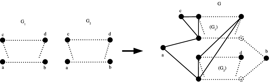
For parallel composition an additional vertex was introduced. It can be done using the following operations (also see Figure 3):
The final step in the construction, after all series and parallel composition have been done, is to connect vertices and and connect vertices and . ∎
The decision version of the hamiltonian cycle problem for graphs of bounded cliquewidth is shown to be polynomial time solvable in [7]. Though bounded treewidth implies bounded cliquewidth we are mainly interested in studying the evaluation version. Evaluation of the hamiltonian and permanent polynomials was shown in [6] to be in for matrices of bounded treewidth. They give efficients algorithms for a much broader class of problems, but the proof we give here is more direct and gives a more precise characterization.
By Definition 6, computing the permanent of a matrix amounts to computing the sum of the weights of all cycle covers of . In our algorithm we need to consider partial covers, which are generalizations of cycle covers.
Definition 7
A partial cover of a directed graph is a union of paths and cycles such that every vertex of the graph belongs to at most one path (and to none of the cycles), or to at most one cycle (and to none of the paths).
The weight of a partial cover is the product of the weights of all participating edges. More generally, for any set of edges the weight of is defined as the product of the weights of the elements of .
In contrast to cycle covers, for a partial cover there is no requirement that all vertices be covered.
The following theorem from [2] is a standard tool in the design of parallel algorithms for graphs of bounded treewidth (see also [3] and [9]).
Theorem 3.4
Let be a graph of treewidth k with n vertices. Then there exists a tree-decomposition of G of width such that is a binary tree of depth at most .
We also need the following standard lemma:
Lemma 1
Let be a circuit of depth . Then there exists a formula of depth and size representing the same polynomial.
Proof
We construct the formula from the circuit by duplicating entire subcircuits whenever we reuse a gate. The formula constructed in this way also has height . In the produced formula the number of gates having distance to the root is at most twice the number of gates having distance to the root, so the formula has at most gates. ∎
Theorem 3.5
The permanent of a matrix of bounded treewidth can be expressed as a formula of size .
Proof
We show how to construct a circuit of depth , which can then be expressed as a formula of size using Lemma 1. Consider the graph and apply Theorem 3.4 to obtain a balanced, binary tree-decomposition of bounded width . For each node of , we denote by the subtree of rooted at , and we denote by the set of vertices of which belong to for at least one of the nodes of . We denote by the subgraph of induced by the subset of vertices .
Consider a partial cover of . Any given edge is either used or unused by . Likewise, any given vertex of has indegree 0 or 1 in , and outdegree 0 or 1. We denote by the list of all these data for every edge and every element of . By abuse of language, we will say that an edge in is used by if it is used by one partial cover satisfying (or equivalently, by all partial cover satisfying ).
We will compute for each possible list a weight , defined as the sum of the weights of all partial covers of satisfying the following three properties:
- (i)
the two endpoints of all paths of belong to ;
- (ii)
all uncovered vertices belong to ;
- (iii)
.
Note that the number of weights to be computed at each node of is bounded by a constant (which depends on ). When is the root of we can easily compute the permanent of from the weights : it is equal to the sums of the over all which assign indegree 1 and outdegree 1 to all vertices of . Also, when is a leaf of we can compute the weights in a constant number of arithmetic operations since has at most vertices in this case. It therefore remains to explain how to compute the weights when is not a leaf.
Our algorithm for this proceeds in a bottom-up manner: we will compute the weights for from the weights already computed for its left child (denoted ) and its right child (denoted ). The idea is that we can obtain a partial cover of by taking the union of a partial cover of and of a partial cover of , and adding some additional edges. Conversely, a partial cover of induces a partial cover of and a partial cover of . In order to avoid counting many times the same partial cover, we must define the considered partial covers of and to ensure that the partial cover of induces a unique partial cover of and a unique partial cover of . We will say that is compatible with if and only if the following holds:
- -
no edge in is used in or ;
- -
for every vertex at most one of assigns indegree 1 to ;
- -
for every vertex at most one of assigns outdegree 1 to ;
- -
every vertex has indegree 1 and outdegree 1 in ;
- -
every vertex has indegree 1 and outdegree 1 in .
We now have to prove two things. If there is a partial cover of which satisfies the properties (i) and (ii) such that then it induces a partial cover of and a partial cover of such that and satisfy (i) and (ii), , , and is compatible with . Conversely, if is compatible with , and and are partial covers of and satisfying (i), (ii), , and , then there exists a unique partial cover of containing and such that .
Consider a partial cover of which satisfies the properties (i) and (ii) defined above. We can assign to a unique triple defined as follows. First, we define as the set of edges of . Then we define as the set of edges of which have their two endpoints in , and at least one of them outside of . Finally, we define as the set of edges of which have their two endpoints in , and at least one of them outside of . Note that since forms a partition of the edges of . Moreover, is a partial cover of and properties (i) and (ii) are satisfied: the endpoints of the paths of and the uncovered vertices of all belong to . Likewise, is a partial cover of and properties (i) and (ii) are satisfied. If and , it is clear that is compatible with . Any other partition of in three parts with one partial cover of , one partial cover of , and a subset of edges in would have an edge of used by or . Hence would not be compatible with .
Suppose now is compatible with , and and are partial covers of and satisfying (i), (ii), , and . We define as the set of edges of which are used by . It is clear that , and are disjoint. Consider . Since is compatible with , is a partial cover satisfying (i) and (ii). It is also clear that is the only partial cover containing and such that .
These considerations lead to the formula
The sum runs over all pairs that are compatible with . The weight can therefore be computed in a constant number of arithmetic operations.
Since the height of is the above algorithm can be executed on a circuit of height as well. ∎
Theorem 3.6
The hamiltonian of a matrix of bounded treewidth can be expressed as a formula of size .
Proof
The proof is very similar to that of Theorem 3.5. The only difference is that we only consider partial cycle covers consisting exclusively of paths, and at the root of the partial cycle covers of the two children must be combined into a hamiltonian cycle. ∎
4 Perfect matchings of planar graphs
In this section we work with undirected graphs.
Definition 8
A perfect matching of a graph is a subset of such that every vertex in is incident to exactly one edge in . The weight of a perfect matching is the product of weights of all edges in . By we denote the sum of weights of all perfect matchings of .
In 1967 Kasteleyn showed in [8] that can be computed efficiently if is planar. His observations was that for planar graphs could be expressed as a special kind of Pfaffian. For general non-planar graphs computing is -complete (or -complete in the boolean model of computation). This follows from the fact that for a bipartite graph , is equal to the permanent of its “bipartite adjacency matrix” (if , is a matrix and is equal to the weight of the edge between and ).
Theorem 4.1
Let be a family of polynomials with coefficients in a field . The three following properties are equivalent:
- •
can be computed by a family of polynomial size weakly skew circuits.
- •
can be computed by a family of polynomial size skew circuits.
- •
There exists a family of polynomial size planar graphs with edges weighted by constants from or variables of such that .
The equivalence of (i) and (ii) is etablished in [13] and [14]. In [13] the complexity class is defined as the class of polynomial families computed by polynomial size (weakly) skew circuits, and it is shown that the determinant is -complete. We have therefore shown that computing for a planar graph is equivalent to computing the determinant. Previously it was known that could be reduced to computing Pfaffians [8]. The equivalence of (iii) with (i) and (ii) follows immediately from Theorem 4.2 and Theorem 4.3.

Theorem 4.2
The output of every skew circuit of size can be expressed as where is a weighted, planar, bipartite graph with vertices. The weight of each edge of is equal to 1, to -1, or to an input variable of the circuit.
Proof
Let be a skew circuit; that is, for each multiplication gate at least one of the inputs is an input gate of (w.l.o.g. we assume it is exactly one). Furthermore, by making at most a linear amount of duplication we can assume all input gates have outdegree 1. Thus, every input gate of is either input to exactly one addition gate or input to exactly one multiplication gate (ignoring the trivial special case where only consist of a single gate), and throughout the proof we will distinguish between these two types of input gates.
Consider a drawing of in which all input gates which are input to an addition gate, are placed on a straight line, and all other gates are drawn on the same side of that line. Assume all arrows in the circuit are drawn as straight lines. This implies at most a quadratic number of places where two arrows cross each other in the plane. By using the planar crossover widget from Figure 4 we replace these crossings by planar subgraphs, introducing at most a quadratic amount of extra gates.
For each multiplication gate we have that exactly one of the input gates is an input gate of , so these input gates can be placed arbitrarily close the the multiplication gate in which they are used. Thus we obtain a planar skew circuit computing the same value as .

Consider a topological ordering of the gates in in which input gates that are input to multiplication gates have numbers less than 1, and input gates that are input to addition gates have the numbers 1 through (where is the number of input gates that are input to addition gates). Let be the number of the output gate in this topological ordering of . Steps 1 through in the construction of are shown in Figure 5. Edge weight denote the input at the gate with topological number in .

For each step an addition or multiplication gate are handled as shown in Figure 6. White vertices indicate vertices that are already present in the graph, whereas black vertices indicate new vertices that are introduced during that step. For multiplications the edge weight denote the value of the input gate of , which is input to that multiplication gate. Finally, the output gate of is handled in a special way.
Correctness can be shown by induction using the following observation. For each step in the construction of the following properties will hold for the graph generated so far: The labels have been assigned to distinct vertices. For all if the vertex with label is removed (along with all adjacent edges), then of the remaining graph equals the value computed at gate with topological number in . It is clear that the graph produced during the initialization (Figure 5) has this property. For the remaining vertices in the topological ordering we either have to simulate an addition gate () or a multiplication gate (). For each new labeled vertex added in this way we can see that it simulates the corresponding gate correctly, without affecting the simulation done by other labeled vertices in the graph.
Bipartiteness of can be shown by putting the vertex labeled as well as vertices labeled , , on one side of the partition, and all other vertices on the other side of the partition. ∎
Remark 2
The theorem can be proven for weakly skew circuits as well without the result from [14] stating that weakly skew circuits are equivalent to skew circuits. Consider the graph . One can show that this graph has a single perfect matching of weight . For simulation of a multiplication gate, instead of adding a single edge of weight , one can add an entire subcircuit constructed in the above manner.
Theorem 4.3
For any weighted, planar graph with vertices, can be expressed as the output of a skew circuit of size . Inputs to the skew circuit are either constants or weights of the edges of .
Proof
The result will be established by computation of Pfaffians and is shown by combining results from [8] and [10].
Let be a weighted graph and an oriented version of . Then the Pfaffian is defined as:
where ranges over all perfect matchings of . The Pfaffian depends on how the edges of are oriented, since the sign of a perfect matching depends on this orientation (details on how the sign depends on the orientation are not needed for this proof).
It is known from Kasteleyn’s work [8] that all planar graphs have a Pfaffian orientation of the edges (and that such an orientation can be found in polynomial time). A Pfaffian orientation is an orientation of the edges such that each term in the above sum has positive sign . So for planar graphs computing reduces to computing Pfaffians (which can be done in polynomial time).
A Pfaffian orientation of does not depend on the weights of the edges, it only depends on the planar layout of . In our reduction to a skew circuit we can therefore assume that a Pfaffian orientation is given along with , thus the problem of computing by a skew circuit is reduced to computing by a skew circuit.
¿From Theorem 12 in [10] we have that can be expressed as where is a weighted, acyclic, directed graph with distinguished source and sink vertices denoted and (recall from Theorem 3.2). The size of is polynomial in the size of .
The last step is to reduce to a polynomial size skew circuit representing the same polynomial. Consider a topological ordering of the vertices of . The vertex is replaced by an input gate with value 1. For a vertex of indegree 1, assume is the vertex such that there is a directed edge from to in , and assume the weight of this edge is . We then replace by a multiplication gate, where one arrow leading to this gate comes from the subcircuit representing , and the other arrow leading to this gate comes from a new input gate with value . Vertices of indegree are replaced by a series of addition gates, adding weights of all paths leading here, similar to what is done for vertices of indegree 1.
The circuit produced in this way clearly represent the same polynomial, and it is a skew circuit because for every multiplication gate at least one of the arrows leading to that gate comes from an input gate. ∎
5 Acknowledgements
This work was done while U. Flarup was visiting the ENS Lyon during the spring semester of 2007. This visit was partially made possible by funding from Ambassade de France in Denmark, Service de Coopération et d’Action Culturelle, Ref.:39/2007-CSU 8.2.1.
References
- [1] A. Barvinok. Two algorithmic results for the traveling salesman problem. Mathematics of Operations Research, 21:65-84 (1996).
- [2] H. L. Bodlaender. NC-algorithms for graphs with small treewidth. In Proc. 14th Workshop Graph-Theoretic Concepts in Computer Science WG’88, p. 1-10. Springer Verlag, Lecture Notes in Computer Science 344 (1989).
- [3] H. L. Bodlaender and T. Hagerup. Parallel Algorithms with Optimal Speedup for Bounded Treewidth. In Z. Fulop and F. Gecseg, editors, Proceedings 22nd International Colloquium on Automata, Languages and Programming, pages 268-279, Berlin. Springer-Verlag, Lecture Notes in Computer Science 944 (1995).
- [4] P. Bürgisser. Completeness and Reduction in Algebraic Complexity Theory. Number 7 in Algorithms and Computation in Mathematics. Springer, 2000.
- [5] B. Courcelle. Graph Grammars, Monadic Second-Order Logic And The Theory Of Graph Minors. Contemporary Mathematics, Volume 147, p. 565-590 (1993).
- [6] B. Courcelle, J. A. Makowsky and U. Rotics. On the fixed parameter complexity of graph enumeration problems definable in monadic second-order logic. Discrete Applied Mathematics, 108:23-52 (2001).
- [7] W. Espelage, F. Gurski and E. Wanke. How to solve NP-hard graph problems on clique-width bounded graphs in polynomial time. Lecture Notes in Computer Science, 2204 (2001).
- [8] P. W. Kasteleyn. Graph theory and crystal physics. In F. Harary, editor, Graph Theory and Theoretical Physics, p. 43-110. Academic Press (1967).
- [9] A. K. Mackworth and Y. Zhang. Parallel and Distributed Finite Constraint Satisfaction. Technical Report 92-30, Department of Computer Science, University of British Columbia, Vancouver, B. C. Canada (1992).
- [10] M. Mahajan, P. R. Subramanya and V. Vinay. The combinatorial approach yields an NC algorithm for computing Pfaffians. Discrete Applied Mathematics 143, p.1-16 (2004).
- [11] J. A. Makowsky and K. Meer. Polynomials of bounded treewidth. Foundations of Computational Mathematics, Proceedings of the Smalefest 2000, Felipe Cucker and J. Maurice Rojas, edts., World Scientific 2002, p. 211-250 (2002).
- [12] G. Malod. Polynômes et coefficients. Ph.D. thesis (2003).
- [13] G. Malod and N. Portier. Characterizing Valiant’s Algebraic Complexity Classes. In MFCS 2006, Proceedings of the 31st International Symposium on Mathematical Foundations of Computer Science, volume 4162 of Lecture Notes in Computer Science, p. 704-716 Springer Verlag (2006).
- [14] S. Toda. Classes of arithmetic circuits capturing the complexity of computing the determinant. IEICE Transactions on Information and Systems, E75-D, p. 116-124 (1992).
- [15] L. G. Valiant. The complexity of computing the permanent. Theoretical Computer Science 8, p.181-201 (1979).
- [16] L. G. Valiant. Completeness classes in algebra. In Proc. 11th ACM Symposium on Theory of Computing, pages 249–261, 1979.
- [17] L. G. Valiant. Reducibility by algebraic projections. In Logic and Algorithmic (an International Symposium held in honour of Ernst Specker), pages 365–380. Monographie 30 de L’Enseignement Mathématique, 1982.
- [18] L. G. Valiant. Holographic algorithms. In Proc. 45th Annual IEEE Symposium on Foundations of Computer Science, IEEE Press, p. 306-315 (2004).