Implications of - Mixing for New PhysicsPreprint: SLAC-PUB-12496 WSU–HEP–0701 UH-511-1104-07
Abstract
We provide a comprehensive, up-to-date analysis of possible New Physics contributions to the mass difference in - mixing. We consider the most general low energy effective Hamiltonian and include leading order QCD running of effective operators. We then explore an extensive list of possible New Physics models that can generate these operators, which we organize as including Extra Fermions, Extra Gauge Bosons, Extra Scalars, Extra Space Dimensions and Extra Symmetries. For each model we place restrictions on the allowed parameter space using the recent evidence for observation of meson mixing. In many scenarios, we find strong constraints that surpass those from other search techniques and provide an important test of flavor changing neutral currents in the up-quark sector. We also review the recent BaBar and Belle findings, and describe the current status of the Standard Model predictions of - mixing.
I Introduction
Meson-antimeson mixing has traditionally been of importance because it is sensitive to heavy degrees of freedom that propagate in the underlying mixing amplitudes. Estimates of the charm quark and top quark mass scales were inferred from the observation of mixing in the and systems, respectively, before these particles were discovered directly.
This success has motivated attempts to indirectly detect New Physics (NP) signals by comparing the observed meson mixing with predictions of the Standard Model (SM). Mixing in the Kaon sector has historically placed stringent constraints on the parameter space of theories beyond the SM and provides an essential hurdle that must be passed in the construction of models with NP. However, anticipated breakthroughs from the B-factories and the Tevatron collider have not been borne out – the large mixing signal in the and systems is successfully described in terms of the SM alone (although the parameter spaces of various NP models have become increasingly constrained). Short of awaiting LHCB and the construction of a super-B facility, there is one remaining example for possibly observing indirect signs of NP in meson mixing, the flavor oscillations. In this case, the SM mixing rate is sufficiently small that the NP component might be able to compete datta. There has been a flurry of recent experimental activity regarding the detection of - mixing babar; belle; staric; babar:2007aa, which marks the first time Flavor Changing Neutral Currents (FCNC) have been observed in the charged quark sector. With the potential window to discern large NP effects in the charm sector bghp; Burdman:2001tf and the anticipated improved accuracy for future mixing measurements, the motivation for a comprehensive up-to-date theoretical analysis of New Physics contributions to meson mixing is compelling.
I.1 Observation of Charm Mixing
The heightened interest in - mixing started with the almost simultaneous observations by the BaBar babar and Belle belle collaborations of nonzero mixing signals at about the per cent level,11 1 Our definitions of the mixing parameters , , and are standard and are given in Eqs. (11),(12).
| (1) | |||
| (2) |
This was soon followed by the announcement by the Belle collaboration of mixing measurements from the Dalitz plot analyses of staric,
| (3) |
A preliminary fit to the current database22 2 An updated fitasner gives the values , . These are essentially unchanged from the HFAG preliminary results given above and used in our analysis; the difference will not affect our numerical results. by the Heavy Flavor Averaging Group (HFAG) gives asner
| (4) |
Since this paper addresses the issue of the mass splitting induced by mixing, our primary concern is with the signal for , seen here to be a 2.4 sigma effect. This is below the generally accepted threshold for “evidence” and is more in the nature of a “hint”. However, we note that a 2.4 sigma effect will automatically have a non-zero lower bound at confidence-level. For the sake of reference, we cite the one-sigma window for the HFAG value of ,
| (5) |
or equivalently for itself,
| (6) |
Let us briefly describe our strategy for dealing with the above HFAG values in light of both SM and NP contributions. We shall argue in Sect. III that the SM predictions, although indeed compatible with the observed range of values for the mixing parameters, contain significant hadronic uncertainties. Moreover, we do not know the relative phase between the SM contribution and that from any NP model, so that will lie between the extreme limiting cases of constructive and destructive interference. In addition, since the observation of mixing is new, the measurements will fluctuate with future refinements in the analyses and as more data is collected. To best deal with these realities, we will present our results by displaying a given NP prediction as a pure NP signal (i.e. as if there were no SM component) and for comparison, display curves of constant for the five values
| (7) |
This (approximately HFAG 2) range reveals the sensitivity of to variations in the underlying NP parameter space. We will then show the present constraints placed on the NP model parameter space, by assuming that the NP contribution cannot exceed the upper bound on . This procedure mirrors that which is traditionally employed in obtaining bounds on NP from - mixing.
I.2 New Physics Possibilities
- mixing at the observed level is much larger than the quark-level (‘short-distance’) SM prediction Golowich:2005pt but is in qualitative accord with hadron-level (‘long-distance’) SM expectations. However, because the latter are beset with hadronic uncertainties, it cannot be rigorously concluded that only SM physics is being detected. In this paper, we will consider a broad menu of NP possibilities. As the operation of the LHC looms near, the number of potentially viable NP models has never been greater. Our organizational approach to analyzing these is to address NP models with:
- 1.
Extra Fermions (Sect. IV)
A: Fourth Generation
B: Heavy Vector-like Quarks
(1): Singlet Quarks
(2): Singlet Quarks
C: Little Higgs Models
- 2.
Extra Gauge Bosons (Sect. V)
A: Generic Z’ Models
B: Family Symmetries
C: Left-Right Symmetric Model
D: Alternate Left-Right Models from E6 Theories
E: Vector Leptoquark Bosons
- 3.
Extra Scalars (Sect. VI)
A: Flavor Conserving Two-Higgs-Doublet Models
B: Flavor Changing Neutral Higgs Models
C: Scalar Leptoquark Bosons
D: Higgsless Models
- 4.
Extra Space Dimensions (Sect. VII)
A: Universal Extra Dimensions
B: Split Fermion Models
C: Warped Geometries
- 5.
Extra Symmetries (Sect. VIII)
A: Minimal Supersymmetric Standard Model
B: Quark-Squark Alignment Models
C: Supersymmetry with R-Parity Violation
D: Split Supersymmetry
In the above, we have chosen to consider only supersymmetry in Sect. VIII due to its extensive literature and to cover other extended symmetries elsewhere in the paper.
Any NP degree of freedom will generally be associated with a generic heavy mass scale , at which the NP interaction will be most naturally described. At the scale of the charm mass, this description will have been modified by the effects of QCD. These should not be neglected, so we perform our NP analyses at one-loop level for the strong interactions. The theoretical background for this is presented in Sect. II.
Finally, in order to place the NP discussion within its proper context, it makes sense to first review SM charm mixing. This is done in Sect. III. The remainder of the paper then amounts to considering charm mixing with lots of ‘extras’. The paper concludes in Sect. IX with a summary of our findings.
I.3 Basic Formalism
Let us first review some formal aspects of charm mixing. The mixing arises from interactions that generate off-diagonal terms in the mass matrix for and mesons. The expansion of the off-diagonal terms in the neutral mass matrix to second order in the weak interaction is
| (8) |
where and are the effective and hamiltonians.
The off-diagonal mass-matrix terms induce mass eigenstates and that are superpositions of the flavor eigenstates and ,
| (9) |
where . The key quantities in mixing are the mass and width differences,
| (10) |
or equivalently their dimensionless equivalents,
| (11) |
where is the average width of the two neutral meson mass eigenstates. Two quantities, and , which are actually measured in most experimental determinations of , are defined as
| (12) |
where the transition rates pertain to decay into final states of definite CP, is the so-called production asymmetry of and (giving the relative weight of and in the sample) and is the strong phase difference between the Cabibbo favored and double Cabibbo suppressed amplitudes Falk:1999ts. The quantities and account for the presence of CP violation in - mixing, with being related to the parameters of Eq. (9) as and a CP-violating phase of (if one neglects direct CP-violation) Bergmann:2000id. In practice, is measured by comparing decays of into a state of definite CP, such as , to decays of into a final state which is not a CP-eigenstate (such as ) whereas is extracted from a time-dependent analysis of the transition Bergmann:2000id.
The states allow for effects of CP violation. However, CP violation in mixing is negligible in the Standard Model and there is no evidence for it experimentally babar; Nir:2007ac; PDG. Many New Physics scenarios contain new phases which can induce sizable CP violation in the meson sector. Nonetheless, a thorough investigation of such effects is beyond the scope of the present paper. Therefore, we shall work in the limit of CP invariance (so that ) for the remainder of this paper. Throughout, our phase convention will be
| (13) |
Then become the CP eigenstates with .
Keeping in mind the neglect of CP-violation and also the phase convention of Eq. (13), we relate the mixing quantities and to the mixing matrix as
| (14) |
where is the weak hamiltonian density for transitions and denotes the time-ordered product. There is no contribution to from the local term, as it has no absorptive part. New Physics contributions to have already been addressed in Ref. Golowich:2006gq, so the primary thrust of this paper will be to focus on .
The next step, in Sect. II, is to expand the time-ordered product of Eq. (I.3) in local operators of increasing dimension (higher dimension operators being suppressed by powers of ).
II Generic Operator Analysis of - Mixing
Though the particles present in models with New Physics may not be produced in charm quark decays, their effects can nonetheless be seen in the form of effective operators generated by the exchanges of these new particles. Even without specifying the form of these new interactions, we know that their effect is to introduce several effective operators built out of the SM degrees of freedom.
II.1 Operator Product Expansion and Renormalization Group
By integrating out new degrees of freedom associated with new interactions at a scale , we are left with an effective hamiltonian written in the form of a series of operators of increasing dimension. Operator power counting then tells us the most important contributions are given by the operators of the lowest possible dimension, in this case. This means that they must contain only quark degrees of freedom. Realizing this, we can write the complete basis of these effective operators, which can be done most conveniently in terms of chiral quark fields,
| (15) |
where the prefactor has the dimension of inverse-squared mass, the are dimensionless Wilson coefficients,33 3 Throughout this paper, we shall denote Wilson coefficients for operators as and those for operators as . and the are the effective operators:
In total, there are eight possible operator structures that exhaust the list of possible independent contributions to transitions. Since these operators are generated at the scale where the New Physics is integrated out, a non-trivial operator mixing can occur when we take into account renormalization group running of these operators between the scales and , with being the scale where the hadronic matrix elements are computed. We shall work at the renormalization scale GeV. This evolution is determined by solving the RG equations obeyed by the Wilson coefficients,
| (25) |
where represents the matrix of anomalous dimensions of the operators in Eq. (II.1) (note the transposition). Eq. (25) can be solved by transforming to the basis where the transpose of the anomalous dimension matrix is diagonal, integrating, and then transferring back to the original basis . At leading order, we have
| (26) |
where is the evolution matrix, obtained from Eq. (25) by
| (27) |
In the above, is the vector containing the diagonal elements of the diagonalized transposed matrix of the anomalous dimensions , is the matrix that diagonalizes and
| (28) |
For completeness, we display the matrix of anomalous dimensions at leading-order (LO) in QCD Ciuchini:1997bw,
We note that Ref. Ciuchini:1997bw also includes the next-to-leading order (NLO) expressions for the elements in the anomalous dimensions matrix. However, we perform our calculations at LO here since the NLO corrections to the matching conditions in the various models of New Physics have generally not been computed.
Due to the relatively simple structure of , one can easily write the evolution of each Wilson coefficient in Eq. (15) from the New Physics scale down to the hadronic scale , taking into account quark thresholds. Corresponding to each of the eight operators () is an RG factor . The first of these, , is given explicitly by
| (38) |
and the rest can be expressed in terms of as
The RG factors are generally only weakly dependent on the NP scale since it is taken to be larger than the top quark mass, , and the evolution of is slow at these high mass scales. In Table 1, we display numerical values for the with TeV and GeV. Here, we compute using the one-loop evolution and matching expressions for perturbative consistency with the RG evolution of the effective hamiltonian.
II.2 Operator Matrix Elements
We will need to evaluate the -to- matrix elements of the eight dimension-six basis operators. In general, this implies eight non-perturbative parameters that would have to be evaluated by means of QCD sum rules or on the lattice. We choose those parameters (denoted by ) as follows,
where , and represents the meson decay constant. By and large, the compensatory -factors are unknown, except in vacuum saturation and in the heavy quark limit; there, one has .
Since most of the matrix elements in Eq. (II.2) are not known, we will need something more manageable in order to obtain numerical results. The usual approach to computing matrix elements is to employ the vacuum saturation approximation. However, because some of the -parameters are known, we would like to introduce a ‘modified vacuum saturation’ (MVS), where all matrix elements in Eq. (II.2) are written in terms of (known) matrix elements of and matrix elements and ,
where we denote as the number of colors and, as in Ref. Golowich:2005pt, define
| (66) |
as well as
| (67) |
In our numerical work, we take , which is the most recent result from the quenched lattice calculation Gupta:1996yt, and use the CLEO-c determination cleoc. We urge the lattice community to perform an evaluation of the parameters defined in Eq. (II.2) for the full operator set relevant to meson mixing.
III Standard Model Analysis
Theoretical predictions of and within the Standard Model span several orders of magnitude. Roughly, there are two approaches, neither of which give very reliable results because is in some sense intermediate between the heavy-quark and light-quark limits. Consider, for example, as given in Eq. (I.3)
To utilize this relation, one inserts intermediate states between the weak hamiltonian densities . This can be done using either quark or hadron degrees of freedom. Let us consider each of these possibilities in turn.
III.1 Quark-level Analysis
The “inclusive” (or quark-level) approach is based on the operator product expansion (OPE). In the limit, where is a scale characteristic of the strong interactions, and can be expanded in terms of matrix elements of local operators datta; inclusive of increasing dimensions suppressed by powers of inverse charm quark mass.

An instructive example concerns a recent analysis of the leading dimension case Golowich:2005pt in which the width difference is calculated in terms of quarks (cf Fig. 1) and the mass difference is then found from dispersion relations. The calculation is carried out as an expansion in QCD, including leading-order and next-to-leading order contributions with
| (68) |
Here, LO and NLO denote only the corrections at that order and not the full quantity computed to that order. Because , experiences no -quark contribution.44 4 We ignore here the -quark contribution to ; its numerical contribution is subleading ( whereas ). This leaves only , and intermediate states contributing to the mixing diagram of Fig. 1. Taking , the mixing loop-functions will depend on . Table 2 examines in detail the loop-functions for and shows the results of carrying out an expansion in powers of . We see that the contributions of the individual intermediate states in the mixing diagram are not intrinsically small – in fact, they begin to contribute at . However, flavor cancellations remove all contributions through for , so the net result is . Charm mixing clearly experiences a remarkable GIM suppression! The corresponding result for turns out to be . Summarizing, the leading dependences in for the dimension six contributions are
| (69) |
| Int. State | |||
|---|---|---|---|
| Total |
The source of this -dependence is understood as follows. The mixing amplitude is known to vanish in the limit, so the breaking of chiral symmetry and of SU(3) flavor symmetry play crucial roles. Thus, a factor of comes from an violating mass insertion on each internal quark line and another from an additional mass insertion on each line to compensate the chirality flip from the first insertion. This mechanism of chiral suppression accounts for the dependence of , and . The case of requires yet another factor of to lift the helicity suppression for the decay of a pseudoscalar meson into a massless fermion pair.
Let us next display the LO expressions for and (to leading order also in ) Golowich:2005pt,
| (70) |
where and are the relevant Wilson coefficients. For our numerical computations, we adopt the values used in Ref. Golowich:2005pt,
| (71) |
Numerical results for the LO and NLO contributions, where a discussion of the NLO effects can be found in Ref. Golowich:2005pt, (cf Table 3) reveal that is given by to a reasonable approximation (due to the dependence discussed above) whereas is greatly affected by destructive interference between and . The net effect is to render and of similar small magnitudes, at least through this order of analysis.
| LO | NLO | LO + NLO (Central Values) | |
|---|---|---|---|
The quark-level prediction of and just described is a result of expanding in terms of three ‘small’ quantities, , , and . As a consequence, the use of an OPE to describe charm mixing is not entirely straightforward because terms suppressed by higher powers of could nevertheless be important if they contained relatively fewer powers of . However, at the next orders in the OPE one encounters corrections multiplied by about a dozen matrix elements of dimension-nine operators and corrections with more than twenty matrix elements of dimension-twelve operators. This introduces a multitude of unknown parameters for matrix elements that cannot be computed at this time. Simple dimensional analysis Bigi:2000wn suggests the magnitudes , although order-of-magnitude cancellations or enhancements are possible.55 5 Any effect of higher orders in or which could produce a contribution in the lowest possible power could yield a dominant contribution to the prediction of and Falk:2001hx; ggp. Although the BaBar and Belle observations of could be ascribed to a breakdown of the OPE or of duality, it is clear that such a large value of is by no means a generic prediction of OPE analyses.
III.2 Hadron-level Analysis
The meson mass is not very large, so one might question whether the OPE approach discussed in the previous subsection can successfully describe - mixing. This is especially so since the leading contribution in the -breaking parameter enters only as a suppressed contribution in the expansion, which implies that one has to deal with a large number of unknown operator matrix elements.
As an alternative, one might consider saturating the correlation functions of Eq. (I.3) with exclusive hadronic states, switching to a purely hadronic description. This approach should be valid as the mass of the meson lies in the middle of a region populated by excited light-quark states. In principle, this “exclusive” (or hadronic) approach should sum over all possible intermediate hadronic multiplets. Since one has to deal with off-shell hadronic states in the calculation of , some modeling is necessarily involved. By contrast, a calculation of in this approach is less model-dependent. The usual approach to computing is to first calculate and then use a dispersion relation to obtain . This is appropriate, as the contribution due to -flavored intermediate states (which appears in but not ) is negligibly small.
One possible approach would be to select a set of, say, two-body intermediate states 66 6 The simplest intermediate state is a single-particle resonance contribution. Preliminary estimates of resonance contributions to - mixing appear to be small Golowich:1998pz, although much remains to be learned about the resonance spectrum in the vicinity of the mass., and write their contribution to mixing in terms of charged pseudoscalar () branching fractions Donoghue:1985hh; lw,
| (72) |
where is as in Eq. (12). One can use available experimental data on two-body branching ratios to estimate their contribution to . A dispersion relation then relates to . However, the example above explicitly shows the cancellations between states that are present within a given multiplet. Such cancellations make this procedure very sensitive to experimental uncertainties. One would need to know the contribution of each decay mode with extremely high precision, and that is simply not feasible at this time. Another possibility is to model decays theoretically Buccella:1994nf. In this reference, was determined in this manner and the result was found. This result is, however, smaller than the recent BaBar and Belle observations.
Clearly, is not sufficiently light for its decays to be dominated by just two-body final states. Multiparticle intermediate states must also be taken into account in - mixing calculations. In doing so, it is convenient to calculate the contribution of each multiplet separately, as symmetry produces substantial cancellations among members of the same multiplet as we saw above. This can be thought of as a long-distance version of the GIM mechanism. The surviving contribution is expected to be of second order in the -breaking parameter Falk:2001hx. Denoting by a value that would take if elements of the final state belonging to representation , or , were the only channels open for D-decay, one can write as a sum over all possible ’s weighted by the -decay rate to each representation,
| (73) |
It is possible to show that can be computed as Falk:2001hx
| (74) |
It should be noted that in the limit of -conservation and retaining phase space differences as the only source of breaking (i.e. neglecting breaking in the matrix elements), can be computed without any hadronic parameters. This is an appropriate approximation, as the main contribution comes from the multiparticle (four-particle) intermediate state multiplets. For those states, there are multi-kaon modes which are kinematically forbidden. In such cases, phase space effects alone can provide enough violation to induce Falk:2001hx. In other words, such large effects in appear for decays near the threshold, where an analytic expansion in violation is no longer possible. It is interesting that such effects from multiparticle states are not reproduced in the OPE calculation, as the resulting contribution does not come from short-distances.
The use of a dispersion relation for then suggests it would receive contributions of a similar order of magnitude as those for Falk:2004wg. An important difference between the resulting values of and is that even retaining phase space differences as the sole contributor to breaking does not insure cancellation of the hadronic matrix elements. However, with some reasonable model-dependent assumptions, one arrives at the conclusion that Falk:2004wg. It is thus reasonable to believe that the observed - mixing is reflecting Standard Model contributions.
III.3 Comments
The above discussions show that, contrary to the system, Standard Model estimates of and for the charm system contain significant intrinsic uncertainties. On the other hand, SM values near those found by BaBar and Belle cannot be ruled out. Therefore, it will be difficult to attribute a clear indication of New Physics to - mixing measurements alone. This means that the only robust signal of New Physics in the charm system would be the observation of large CP violation, which we will not consider here. Nonetheless, a thorough analysis of indirect New Physics contributions is of value, and we find that large regions of parameter space can be excluded in many models, placing additional restrictions on model building. This will be useful in conjunction with corresponding direct searches for New Physics at the LHC.
In what follows, we will take the approach that the New Physics contributions cannot exceed the 1 experimental upper bound for . Keeping in mind that this upper limit is likely to change as data samples increase and analyses mature, we also display the effects of on the parameter space of New Physics scenarios. These values are to be used as a guide for how our resulting constraints may change in the future. In addition, we will neglect the errors on the determinations of the meson decay constant and B-factors; this will have a small effect on our results given the present large uncertainty in the experimental determination of - mixing. In all cases, we will neglect the possibility of interference between the SM and New Physics contributions. We now turn to the examination of various scenarios for physics beyond the SM.
IV Extra Fermions
The quark sector of the Standard Model can be modified in several ways, and new fermions are predicted to exist in many extensions of the SM. They can be classified according to their electroweak quantum number assignments; here we consider the possibilities of a sequential fourth generation quark doublet (Sect. IV.1), heavy quark iso-singlets (Sect. IV.2) and non-SM quarks associated with Little Higgs models (Sect. IV.3). The contributions of such heavy quarks can remove the efficient GIM cancellation inherent in the short distance SM computation and can give rise to - mixing at the level of the current experimental limit.
IV.1 Fourth Generation Quark Doublet
A simple extension to the Standard Model is the addition of a fourth family of fermions. Precision electroweak data severely constrains this possibility. The Particle Data Group PDG quotes a restriction on the number of families to be from the oblique parameter Peskin:1991sw alone. We note, however, that the LEP Electroweak Working Group LEPEWWG allows for a more generous range of the parameter from their electroweak fit. In either case, this restriction can be relaxed by allowing the parameter to vary as well, or by adding other sources of new physics which would participate in the electroweak fit such as an extended Higgs sector He:2001tp. The requirement of anomaly cancellation implies the existence of a fourth lepton family as well (almost degenerate to satisfy the constraint with ) or an extra right-handed quark doublet. Direct collider searches by the CDF and D0 Collaborations at the Tevatron currently place a bound PDG on the mass of a charged fourth generation quark of GeV if the -quark decays respectively via charged current interactions into leptons + jets, via FCNC with , or is quasi-stable. We recall that perturbative unitarity considerations Chanowitz:1978uj in scattering restricts the mass of sequential heavy flavors to be GeV.
Here, we review the contribution of a fourth generation of quarks to mixing, keeping in mind that some other New Physics may also be present in order to evade the precision electroweak constraints and that it also may or may not contribute to the mixing. The primary motivation for this discussion is to set up the formalism that will be used in the following Sections.
The fourth generation quark contributes to mixing via a box diagram which also contains the SM bosons. Note that since the -quark is not kinematically accessible in charm-quark decay, it will not contribute to the dispersive amplitude for in Eq. (I.3). The hamiltonian at the mass scale in the fourth generation model is q4
| (75) |
where are the well-known Inami-Lim functions Inami:1980fz (given in the Appendix), , , and the sum runs over the internal quark flavors. As discussed in the previous Section, there is a strong GIM cancellation in meson mixing, which leaves a sizable contribution only from the heavy quark and sets in the above sum. Performing the RG evolution, we obtain at the scale
| (76) |
which in turn gives
| (77) |
It should be noted that for , only contributions below are required.
The value of as a function of the CKM mixing elements is displayed in Fig. 2 for various values of the -quark mass. We see that the experimental limit of places sizable constraints in the -quark mixing-mass parameter space. We also show the exclusion contours for possible future experimental bounds of (corresponding to the blue dashed, red dashed, cyan dotted, and green dot-dashed curves, respectively) as discussed in the Introduction. We note that the present constraints on the CKM mixing parameters are an order of magnitude stronger than those obtained from unitarity considerations PDG of the CKM matrix.


Right: The present excluded region in the mass-mixing parameter plane, as well as possible future contours taking , corresponding to the blue dashed, red dashed, cyan dotted, and green dot-dashed curves, respectively.
IV.2 Heavy Vector-like Quarks
The next possibility of interest is the presence of heavy quarks which are singlets (so-called vector-like quarks) branco. We will consider both charge assignments and for the heavy quarks. Both choices are well motivated, as such fermions appear explicitly in several models of physics beyond the Standard Model. For example, weak isosinglets with appear in GUTs q2; jlhtgr, with one for each of the three generations (, , and ). Weak isosinglets with occur in Little Higgs theories q3a; q3b in which the Standard Model Higgs boson is a pseudo-Goldstone boson, and the heavy iso-singlet quark cancels the quadratic divergences generated by the top quark in the mass of the Higgs boson.
IV.2.1 Singlet Quarks
We first consider the class of models with down-type singlet quarks. For this case, the down quark mass matrix is a array if there is just one heavy singlet (or for three heavy singlets as in models). As a consequence, the standard CKM matrix is no longer unitary. Moreover, the weak charged current will now contain terms that couple up-quarks to the heavy singlet quarks. For three heavy singlets, we have
| (78) |
where and refer to the standard up quark and heavy isosinglet down quark sectors. The are elements of a matrix, which is the product of the and unitary matrices that diagonalize the and quark sectors, respectively. The resulting box diagram contribution to from these new quarks is displayed in Fig. 3.

Assuming that the contribution of one of the heavy quarks (say the quark) dominates, one can write an expression (similar to that in Eq. (77)) for q4,
| (79) |
where and for large . The light-heavy mixing angles should go as for large to keep the contribution under control. The current bound on from unitarity of the CKM matrix is not very stringent, PDG. An -quark mass in the range 0.2 to 1 TeV gives rise to a mixing contribution that can exceed the current experimental limit in Eq. (4). Hence a singlet heavy quark of charge can give rise to near the current experimental limit.
In the -based model proposed by Bjorken et al q7, the mass matrix has an especially simple form. The resulting mass matrix has a pseudo-orthogonality property which implies that the CKM matrix, although not unitary, satisfies
| (80) |
The analog of this condition in the up quark sector does not hold, and as a result, there are no new FCNC effects in the down quark sector. For - mixing, the prediction is now that (recall capital lettering is used to denote the heavy quark)
| (81) |
where and is the (small) mixing parameter describing the mixing between the light quark and the heavy quark. Using the experimental values in Eq. (4), we can place bounds on for a given mass , e.g. for TeV. We present the constraints on vs. in Fig. 4.


Right: The present excluded region (short-dashed curve) in the mass and mixing angle parameter plane for the singlet quark in the model of Bjorken et al. q7 described in the text. Possible future contours are also shown, taking from top to bottom, corresponding to the solid, medium dashed, long dashed, and longer dashed curves, respectively.
IV.2.2 Singlet Quarks
Next, consider the possibility of weak isosinglet quarks having charge . These are present in some theories beyond the SM, including for example, Little Higgs models which will be discussed in more detail in the following section. Here, we present the general formalism for this scenario.
The presence of such quarks violate the Glashow-Weinberg-Paschos naturalness conditions for neutral currents gw77. Since their electroweak quantum number assignments are different than those for the SM fermions, flavor changing neutral current interactions are generated in the left-handed up-quark sector. Thus, in addition to the charged current interaction
| (82) |
there are also FCNC couplings with the boson branco,
| (83) |
Here, is a mixing matrix with running over , , and with the CKM matrix comprising the first block.

In this case, a tree-level contribution to is generated from -exchange as shown in Fig. 5. This is represented by an effective hamiltonian of the form
| (84) |
where unitarity demands
| (85) |
Taking the 1 ranges for the experimentally determined values of the CKM elements PDG yields the constraint . This hamiltonian is just a particular case of a more general relation appearing in the following section.77 7 The specific correspondence is , and . The QCD running from to for this effective hamiltonian is trivial, leading to
| (86) |
where it should be noted that for , only contributions below are required. This hamiltonian leads to
| (87) |
We present this contribution to from models with a singlet quark in Fig. 6. Note that the bound on the mixing from - mixing is roughly two orders of magnitude better than that from unitarity constraints of the CKM matrix.

IV.3 Little Higgs Models
Little Higgs models q3a; q3b; morelh feature the Higgs as a pseudo Nambu-Goldstone boson of an approximate global symmetry that is broken by a vacuum expectation value (vev hereafter) at a scale of a few TeV. This approximate symmetry protects the Higgs vev through one-loop order relative to the ultra-violet (UV) cut-off of the theory which appears at a higher scale. The breaking of this symmetry is realized in such a way that the Higgs mass only receives quantum corrections at two-loops. In these models the one-loop quadratic divergent contributions to the Higgs mass in the SM are canceled by a new particle of the same spin. These models thus predict the existence of new charged vector-like quarks, gauge bosons, and scalars at the TeV scale.
The most economical model of this type, in that it introduces the minimal number of new fields, is known as the Littlest Higgs q3a; q3b. It is based on a nonlinear sigma model with global symmetry that is broken to the subgroup by a vev . is generated by strongly coupled physics at the UV scale TeV. The fourteen Goldstone bosons remaining after this symmetry breaking yield a physical doublet and complex triplet under , which remain massless at this stage. The contains a gauged subgroup which is also broken by to the SM electroweak gauge group. The remaining four Goldstone bosons are then eaten by a Higgs-like mechanism and give mass, of order TeV, to the gauge fields of the broken subgroups. Masses for the complex triplet are generated at the TeV scale by one-loop gauge interactions. The neutral component of the complex doublet plays the role of the SM Higgs, which receives its mass at two-loops from a Coleman-Weinberg potential, giving . Thus the natural scale for is around a TeV; if is much higher, the Higgs mass must again be finely tuned and this model no longer addresses the hierarchy problem.
The minimum physical spectrum of this model below a TeV is thus that of the SM with a single light Higgs. At the TeV scale, there are four new gauge bosons (an electroweak triplet and singlet), the scalar triplet, and a single vector-like quark . Other variants of Little Higgs models may expand this particle content at the TeV scale.
In general, the new vector-like quark can contribute to - mixing. Since it has different electroweak quantum numbers from the quarks in the SM, FCNC interactions will be induced in the left-handed up quark sector. This generates a tree-level boson exchange contribution to mixing as depicted in Fig. 5. This was considered in Ref. Lee:2004me, where a specific ansatz for the up quark mass matrix was employed, leading to a quite small contribution to . In general, however, one expects the quark mixing to be of order and the contribution of the flavor-changing interaction induced by the existence of the quark can be sizable, as discussed in the previous section. Current data can be used to constrain the mass and mixing of the quark, and the results in Fig. 6 are applicable in this case. Tree-level contributions to mixing with the exchange of the new heavy neutral gauge bosons will likewise be generated, as the fermionic coupling for these fields is also proportional to the fermion’s third component of weak isospin. The operator structure is exactly the same as that given in the previous section, but the magnitude of these contributions will be suppressed relative to the SM boson exchange by the heavy mass of the new neutral gauge bosons. In addition, there could also be new contributions to rare meson decays, as discussed recently in the work of Chen et al. Chen:2007yn.
It has been shown lhewp that a global fit to the precision electroweak data set places a significant limit, which is roughly parameter independent, on the vev in the Littlest Higgs model of TeV. Variants of this model, employing different global symmetries, can reduce this constraint somewhat lhewp2. In addition, a discrete symmetry, called T-parity, can be introduced tparity to alleviate the electroweak bounds. This symmetry is analogous to R-parity in supersymmetry and has the consequence that T-parity is conserved in interactions and that the lightest T-odd particle is stable. This provides a natural Dark Matter candidate in these models. Recent work by Hill and Hill hillhill has shown that anomalies in topological interactions can break this discrete symmetry and thus T parity is no longer an exact symmetry; the resulting phenomenology has yet to be worked out. However, the Ultra-Violet (UV) completion of the theory may or may not allow for the terms which break T-parity, and thus a general statement on the presence of this discrete symmetry in the low-energy theory cannot be made.
In addition to the tree-level contribution discussed above, Little Higgs models with T parity can give rise to a loop contribution to - mixing involving the exchange of the heavy gauge bosons and new mirror fermions, which are present in this form of the model. In fact, three vector-like doublets of mirror fermions are introduced in Little Higgs models with T parity in order to evade compositeness constraints tparity. The effective hamiltonian relevant to - mixing for this contribution is Hubisz:2005bd
| (88) |
Here, corresponds to the relevant elements of the weak mixing matrix in the mirror fermion sector which parameterizes the flavor interactions between the SM and mirror fermions. The quantity (given in the Appendix) is the loop function computed in Ref. Hubisz:2005bd; it depends on , where is the mass of the mirror quark doublet and represents the heavy charged gauge boson mass. The operator appears since the heavy gauge bosons have purely left-handed interactions. The RG running of this hamiltonian is trivial and leads to a factor of . The resulting contribution to the mass difference is
| (89) |
This has recently been computed in Ref. Blanke:2007ee in light of the recent experimental measurement of - mixing, where it is found that this contribution can saturate the experimental bounds.
In Little Higgs models with T parity, there is an additional tree-level contribution arising from the interaction vertex where represents either of the heavy neutral gauge fields and is the odd T-parity quark. couples to the weak eigenstate of the T-parity even quark , which receives its mass from the same Yukawa term that is responsible for the up quark masses. This induces mixing between the quarks in the up quark sector, resulting in FCNC interactions of the SM quarks with the exchange of the new heavy neutral gauge fields. The generic formalism for this contribution will be discussed in the next section, however this particular contribution is thought to be small Hubisz:2005bd.
V Extra Gauge Bosons
Many theories with physics beyond the SM have extended electroweak gauge symmetries, whose hallmark are the existence of new heavy neutral and charged gauge bosons. We note that scenarios with extended gauge symmetries also generally contain new fermions which are required for anomaly cancellation, as well as an extended Higgs sector to facilitate the extended symmetry breaking. The additional heavy gauge bosons are produced directly at hadron colliders via the Drell-Yan mechanism, and the search limit on the masses of new gauge bosons with SM couplings is approaching 1 TeV from Run II data at the Tevatron. The lower bound on the mass of a SM-coupled is 923(965) GeV from CDF(D0) tevzp. The LHC will be able to search for these particles with masses up to TeV tgrtasi. There are many such models that yield large FCNC effects in the up-quark sector.
V.1 Generic Models
It is possible that a new heavy boson has flavor changing couplings in the up quark sector. Here, we examine a generic tree-level FCNC interaction that mediates mixing via -exchange, analogous to the transition depicted in Fig. 5. While the discussion presented here is quite general, many string-inspired models have extra gauge symmetries that lead to extra -bosons with possible flavor-changing couplings jlhtgr; Langacker:2000ju; Arhrib:2006sg.
The effective four-fermion hamiltonian just below the scale is
| (90) |
where the dimensionless flavor changing couplings are the model dependent inputs to the calculation. This is the most general effective hamiltonian and assumes flavor-changing interactions occur in both the left- and right-handed sectors. We first perform a general analysis and will then consider some particular occurrences of a in the Sections below.
We introduce the Wilson coefficients by matching at the mass scale,
| (91) |
with all other Wilson coefficients being zero at this scale. Assuming that and performing the RG running of Eq. (90), we obtain the effective hamiltonian at the scale ,
| (92) |
with
| (93) |
The presence of in Eq. (92) is due to operator mixing in the RG running. Finally, as a check note that for the case of no evolution () we obtain the expected behavior .
Upon evaluating the -to- matrix elements, we obtain the tree contribution to ,
| (94) | |||||
Eq. (94) can be used to relate the input parameters of models ( and ) to some value of . Taking , particularly simple expressions are obtained for the limiting cases:
- 1.
(the case with replaced by yields identical limits):
(95) - 2.
:
(96) where .
In the above, we have fixed the slowly varying and at the middle of their ranges. The results in Eqs. (94)-(96) which constrain combinations of the flavor-changing couplings and the mass (see Fig. 7), can be applied to fit the needs of the NP model builder. For example, in Eq. (95) the choice , implies TeV or alternatively taking TeV yields88 8 After the work described in this section was completed, we received Ref. hv in which similar results were discussed. the bound .

V.2 Family Symmetries
One class of new physics possibilities to be explored in the TeV range is family (horizontal) symmetries. The gauge sector of the Standard Model lagrangian,
| (97) |
actually exhibits a very large global symmetry viz. . The hope is then that some subgroup of this large symmetry is shared by the Higgs sector and the gauge symmetry of the full lagrangian becomes . The group acts on the families horizontally Wilczek:1978xi, and , of course, eventually has to be broken, preferably spontaneously.
The symmetry can be implemented locally, so there will be flavor-changing interactions mediated by new gauge bosons. The symmetry is broken spontaneously, making the gauge boson massive with new scalar fields being introduced in addition to the standard Higgs field.
As a prototype, let us consider a very simple model Monich:1980rr. We consider the group acting only on the first two left-handed families (it may be regarded as a subgroup of an , which is broken). Spontaneous breaking of makes the gauge bosons massive. The LH doublets
| (98) |
transform as under , as do the lepton doublets
| (99) |
and the right-handed fermions are singlets under . The superscript refers to the fact that these are weak eigenstates and not mass eigenstates. The couplings of fermions to the family gauge bosons is given by
| (100) |
where denotes the coupling strength and are the generators of . We define the mass basis by
| (101) |
In the limit of CP-conservation each of the three matrices , , and is characterized by one angle: , , and (where the Cabibbo angle is ). One then finds for the couplings in the fermion mass basis:
| (102) | |||||
For simplicity we assume that after symmetry breaking the gauge boson mass matrix is diagonal to a good approximation in which case are physical eigenstates and any mixing between them is neglected. This lagrangian clearly introduces tree-level FCNC interactions and gives a contribution to - mixing of
| (103) |
A simple symmetry breaking pattern (see, e.g., Monich:1980rr) leads to . Since the effective hamiltonian only involves the operator , the RG-running is simple and leads to the following structure at the scale,
| (104) |
where is the smaller of the new gauge boson masses and . This leads to a value for of
| (105) |
Using the available experimental data on - mixing parameters, yields constraints on the masses of the family symmetry-mediating gauge bosons. They are presented in Fig. 8 for .

V.3 Left-Right Symmetric Model
A puzzling feature of the SM is the left-handed nature of the electroweak interactions. A long-standing possible remedy, known as the Left-Right Symmetric Model (LRM) mohap, seeks to restore parity at high energies by enlarging the gauge symmetry to . This model can be embedded into an (or ) GUT structure which then provides a natural mechanism (seesaw) for generating light neutrino masses. A supersymmetric version of a left-right symmetric GUT model yields the correct prediction tgrdesh for and , while allowing for the masses of the new gauge bosons ( and ) associated with the symmetry to be of order a few TeV or less. Light masses for the new gauge bosons can also be obtained in models with a horizontal symmetry Kiers:2005gh. Manifest left-right symmetry dictates that the right-handed gauge coupling take on the same value as the left-handed SM coupling and that the elements of the right-handed CKM matrix be equal to their left-handed counterparts. In this case, the direct search for new gauge bosons at the Tevatron places the bound tevzp of GeV on the mass of the charged right-handed gauge boson.
The has flavor conserving couplings in this model, and thus does not mediate - mixing. The charged right-handed gauge field, however, can participate in virtual exchange in a box diagram, in association with the SM quarks, and gives a contribution to meson mixing. In fact, the strongest bound on the mass of the , which is TeV in the limit of manifest left-right symmetry, is derived from its contribution to - mixing irvine.
However, there is no compelling theoretical reason to adopt manifest left-right symmetry and in more general models the elements of the right-handed analog of the CKM matrix can take on any values, while still respecting unitarity. In addition the ratio of gauge couplings can vary cmp between . In this case where manifest left-right symmetry is dropped, the bounds from Kaon mixing are softened to GeV langsar and the direct collider searches are significantly weakened tgrwr.
The hamiltonian at the right-handed mass scale is given by
| (106) |
with , , denote the left- and right-handed CKM matrix, and the quantities (an Inami-Lim function) and are given in the Appendix. The first term in this hamiltonian corresponds to the exchange of one and one Standard Model boson in the box diagram, while the second term represents the contribution where only the participates. Here, we ignore mixing between the left- and right-handed gauge bosons. The identification of the matching conditions at the high scale, , are obvious. The RG evolution to the charm scale yields the effective hamiltonian at
| (107) |
where operator mixing has induced the dependence on similar to the generic case discussed above, with
| (108) | |||||
Evaluating the hadronic matrix elements yields
| (109) |
upon employing the vacuum saturation approximation and taking in Eq. (67).
It is clear that in the case of manifest left-right symmetry, the combination of the small CKM elements and the suppression will result in a very small value for . However, it is possible that for non-manifest left-right symmetry, where the right-handed CKM elements may take on larger values, that a significant effect may be generated. We examine this scenario, taking to lie in the range , where is the maximum value that this quantity can attain while respecting unitarity of the right-handed CKM matrix. Our results are shown in Fig. 9 for various values of , taking . We see, that even for the most extreme values of the parameters, the LRM contribution to - mixing never reaches the experimentally determined value. Since both of the loop functions and go as , the suppression from the small internal quark masses dominates this result. The dip in the curves results from interference due to operator mixing.
This exercise shows that a generic scenario with a new heavy charged gauge boson that participates in the box diagram for mixing will not induce sizable contributions to the neutral meson mass difference, unless it is accompanied by new heavy quarks. The recently proposed Twin-Higgs models roni, which are based on a gauge symmetry, contain an extended top quark sector with heavy quarks and would give significant contributions to mixing, but not to .

V.4 Alternate Left-Right Model from Theories
An alternative to the conventional Left-Right Symmetric Model discussed above is possible in supersymmetric Grand Unified Theories jlhtgr. This model is also based on the low-energy gauge group , but makes use of ambiguous fermion assignments within the fundamental representation of Babu:1987kp. The additional right-handed charged and neutral gauge fields in this model have different properties than in the traditional scenario. A single generation in theories contains 27, 2-component fermions (in contrast to the 16 fermions per generation in SO(10)), and quantum number ambiguities arise that allow the assignments to differ from their customary values for the , and fields. In the quark sector, the right-handed up-quarks then form doublets with the exotic vector singlet quark, , that is present in the representation of , while the doublet remains unchanged. and are then singlet fields under all gauge symmetries. This allows, for example, the right-handed boson to couple the right-handed up-quark sector to the singlet quark . Examination of the superpotential for this model shows that the takes on the quantum number assignment of a leptoquark, while the carries negative R-parity and non-zero lepton number, and thus cannot mix with the of the SM or couple to the down-quark sector. The usual constraints on right-handed gauge bosons from the mass difference and polarized decay are thus evaded in this scenario.
These exotic particles can induce significant contributions to - mixing Ma:1987ji via and exchange in a standard box diagram. Note that since the heavy quarks are not kinematically accessible in charm-quark decay, there is no dispersive amplitude in this case. The interactions of the right-handed boson take the form
| (110) |
where are generational indices and is the right-handed analog of the CKM quark mixing matrix governing the right-handed charged currents. The effective hamiltonian at the scale of the right-handed interactions is
| (111) |
where the sum over extends over the three generations of quarks, are the standard Inami-Lim functions Inami:1980fz (given in the Appendix) and with being the mass of the new right-handed gauge boson. Note that this expression mirrors that in Eq. (75) except for the presence of the right-handed operator . Matching at the scale yields
| (112) |
Performing the RG evolution we obtain at the charm quark scale
| (113) |
with . This yields the contribution to the meson mass difference
| (114) |
The magnitude of these contributions is determined by the form of the right-handed quark mixing matrix, the degeneracy of the 3 generations of quarks, as well as the right-handed mass scale. If the quarks are fully degenerate, then a right-handed GIM mechanism is operative due to the unitarity of and this contribution to mixing vanishes. If there are mass splittings between the three generations of , then the observed value of mixing can place bounds on the size of these splittings. Here, we will examine the case where takes on the form of the left-handed quark mixing matrix, i.e., it displays the hierarchal structure of the CKM matrix, and derive constraints on this mass splitting as a function of the right-handed mass scale. Our results are presented in Fig. 10. The value of as a function of , the mass of the right-handed charged gauge boson is displayed for various mass splittings, , where is taken to be constant between the first and second as well as second and third generations. We also display the constraints the present experimental bound of , as well as contours for future possible values of , places on the - mass splitting parameter plane. The results are shown for two representative values of the first generation -quark mass, and 2000 TeV. We see that the mass of the is restricted to be for large values of the quark mass splittings.


Right: The present excluded region in the - mass splitting parameter plane, as well as possible future contours taking , corresponding to the blue dashed, red dashed, cyan dotted, and green dot-dashed curves, respectively. The mass of the first generation singlet quark is taken to be 500 and 2000 GeV as labeled.
V.5 Vector Leptoquark Bosons
In most recent papers on the subject, scalar leptoquarks (particles with both quark and lepton quantum numbers) have usually been associated with -parity-violating SUSY scalars (to be considered in Sect. VIII.3). However, vector leptoquarks (VLQs) are also a possibility brwlq. For example, they naturally arise in Grand Unified Theories, where quarks and leptons belong to the same multiplet Ross:1985ai. Many New Physics models where leptoquarks are introduced as fundamental vector particles imply that they serve as gauge particles mediating quark and lepton-number-changing interactions resulting from GUT-model symmetry groups. Those symmetries are usually broken at a rather high scale, of order GeV, which implies that, barring fine-tuning, vector leptoquarks receive masses near the GUT symmetry-breaking scale. Yet, some models exist where leptoquarks receive masses at a lower scale. In addition, more exotic constructions, such as preon (composite) models, could also contain vector leptoquarks. In those models, however, leptoquarks are composite particles with masses that are of the order of compositeness scale. Thus, observations of effects of VLQs could potentially probe physics at a very high mass scale. It is for these reasons vector leptoquarks are searched for experimentally. Collider searches at the Tevatron for the direct production of vector leptoquark pairs yield the constraint GeV d0lq from Run I data for second generation leptoquarks which decay into muons.
While there are a number of phenomenological studies of vector leptoquarks Davidson:1993qk; Leurer:1993qx, a general problem exists with placing constraints on VLQs from indirect measurements, and in particular from - mixing. This is because their couplings are model-dependent. In particular, loop calculations with massive composites, i.e. non-gauge leptoquarks, receive contributions that are divergent and must be regulated by the compositeness scale. For the case of gauge leptoquarks, and in the absence of a GIM-like mechanism in the leptoquark box diagram, one can choose a gauge (such as the Feynman gauge) to unambiguously compute the effects of leptoquark interactions. In that gauge, however, one also must add contributions from unphysical states responsible for the generation of the VLQ masses. In a specific model, the interactions of the unphysical states are fixed and their contributions are readily computable. However, this then becomes a rather model-dependent procedure because VLQ masses can be generated by various means, including some version of the Higgs mechanism, or a Frogatt-Nielsen mechanism, etc. Rather than rely on a specific model, in what follows, for generality, we shall follow the approach of Ref. Davidson:1993qk and obtain bounds on the couplings of gauge VLQs by dropping the contributions from the unphysical states.
In general, a VLQ could couple to both left-handed and right-handed fermions, so we shall assume the general form of the coupling. We note, however, that there are stringent bounds muchado from low-energy data if leptoquarks couple to both left- and right-handed states, and it is generally assumed that their couplings are chiral. For a quark of flavor and a lepton , we adopt the interaction vertex , which leads to the contribution to meson mixing,
| (115) | |||||
where , and we neglect corrections in the last line. The resulting bounds on VLQ interactions are displayed in Fig. 11.


Right: The present excluded region in the vector leptoquark mass - coupling parameter plane, as well as possible future contours taking , corresponding to the blue dashed, red dashed, cyan dotted, and green dot-dashed curves, respectively.
VI Extra Scalars
No known physical principle restricts the number of Higgs multiplets that can participate in electroweak symmetry breaking. In fact, several theories beyond the SM, such as Supersymmetry and those with extended gauge sectors, require an enlarged Higgs sector in order to break the additional symmetries. Here we examine the effect in - mixing of models with multiple Higgs doublets, with and without flavor conservation, Higgsless models and models with scalar leptoquarks.
VI.1 Flavor Conserving Two-Higgs-Doublet Models
A simple extension of the SM is to enlarge the Higgs sector by one additional doublet. We first examine two-Higgs-doublet models that naturally avoid tree-level FCNC be requiring that all fermions of a given charge receive their masses from only one Higgs doublet gw77. In one such model, known in the literature as Model II, one doublet () gives mass to the up-type quarks, while the down-type quarks and charged leptons receive their mass from the other doublet . This is the scenario that is present in supersymmetric theories and is in fact required by supersymmetry in order to generate masses for all the fermions. Another model, known as Model I, imposes a discrete symmetry such that one doublet () generates masses for all fermions and the second () decouples from the fermion sector In both cases, each doublet receives a vacuum expectation value , subject to the constraint that . There are five physical scalars in these models, , and . The charged Higgs boson can participate in the box diagram for in exchange with the SM quarks as shown in Fig. 12. The interactions with the quark sector are governed by the lagrangian
| (116) |
with in both models and in Model I(II), where . The can have a large contribution bsg to the rare decay , and in Model II the branching fraction for this process sets the bound bsg2 GeV at 95% C.L.. This constraint is relaxed when other sources of New Physics also contribute to , such as in supersymmetry. In this case, the lower limit on the charged Higgs mass is 78.6 GeV from LEP II data PDG.

It is clear that the contributions to from the first term in this lagrangian (which are proportional to ) will only be sizable for extremely small values of ; this region is, however, already excluded bhp from, e.g., and - mixing. In addition, since the contributions in Model I go as multiplied by small mass factors, the effects in this case are also restricted to be small. However, the term proportional to in Model II has the potential to generate a significant contribution to mixing in the large limit. We will thus work in this limit here. Restrictions on the size of can be obtained by requiring that the coupling remain perturbative. If we demand that this coupling not exceed the value of the strong coupling constant, , we find that .
The effective hamiltonian governing meson mixing in the large limit takes the form
| (117) |
where as usual, , the sum extends over , the loop functions can be found in Ref. bhp and are given in the Appendix. The operator structure is the same as in Eq. (75); here, the operator appears due to the presence of the fermion propagator. Note that this structure is quite different than for the case of mixing gino in the large limit. This is simply due to the helicity structure of the couplings when the charged quarks are internal. The QCD evolution to the charm quark scale is simple and results in the factor of . The resulting contribution to the mass difference is
| (118) | |||||
Our results for are displayed in Fig. 13 as a function of for various values of the charged Higgs mass. We see that the effect is quite small and even at large values of the contributions from this model are at least an order of magnitude below the experimental observation.

In the down quark sector, sizable effects in and meson mixing are obtained in the large limit from a double penguin contribution with neutral Higgs exchange gino as depicted in Fig. 14. In this limit, an effective Yukawa interaction is induced for the down type quarks which includes a contribution from the large Yukawa coupling of the top quark. This generates sizable one-loop FCNC couplings for the neutral Higgs in the down quark sector. While the same effects occurs in the up quark sector, the term that becomes significant at large is now proportional to the down quark Yukawa coupling and hence does not generate a sizable effect in - mixing

VI.2 Flavor Changing Neutral Higgs Models
It is well known that the existence of multiple Higgs doublets can lead in general to tree level FCNC transitions gw77. In the down quark sector, there are severe constraints on such couplings from Kaon decays, but these do not necessarily lead to equally strong restrictions in the up-quark sector.
The phenomenological requirement that FCNC effects in the down-strange sector must be very small can be met in a variety of ways. For example, the imposition of global symmetries can make FCNC vanish without affecting the sector fcnch. Another example is the Cheng-Sher ansatz Cheng:1987rs, where the flavor changing couplings of the neutral Higgs bosons are given by , with the being the relevant fermion masses and representing a combination of mixing angles.
To keep our initial discussion general, we allow for Higgs scalars, which have the interactions in the up quark sector
| (119) |
where represents the left-handed quark doublet and is the singlet state. If is the mass of the lightest physical Higgs with flavor-changing couplings, the most general effective four-fermion hamiltonian just below the scale is
| (120) |
where the couplings are model-dependent parameters. As shown in Ref. hw,
| (121) | |||||
at the scale. Here, refers to the mixing matrix which rotates the Higgs doublets to their neutral physical eigenstates. Matching at the Higgs mass scale relates the Wilson coefficients to the three couplings via
| (122) |
with all other Wilson coefficients being zero. Assuming that for all and computing the evolution of Eq. (120) to we obtain
| (123) |
with
| (124) | |||||
The Higgs tree-level contribution to is found by evaluating the -to- matrix element, which gives
| (125) |
where, again, we have used Eqs. (II.2),(67). Together with Eqs. (122),(124), the above can be used to constrain the lightest Higgs mass and associated couplings. As an example, let us assume that at the Higgs mass scale in Eq. (120) and is the effective mass of the N Higgs scalars. In that case, the restriction on possible values of the effective Higgs mass are presented in Fig 15.

We now return to the specific case of the Cheng-Sher ansatz. Here, the neutral Higgs bosons can contribute to through tree-level exchange as well as mediating meson mixing by and t-quark virtual exchange in a box diagram. The restrictions placed on the parameter space of this model from the tree-level contribution are computed as described above, and are presented for an effective Higgs mass as a function of the coupling parameter in Fig. 16. We see that the form of the couplings, being proportional to the light quark masses, result in reduced limits compared to those in Fig. 15 for the general case. The box contribution with , t-quark exchange is described by the effective hamiltonian just below the scale of
| (126) |
where , is given in the Appendix, and the vector operators are generated from the fermion propagators. The RG evolution and evaluation of the matrix elements yields
| (127) |
The resulting constraints from this contribution are displayed in Fig. 16 in the effective Higgs mass - coupling parameter plane. We see that this box contribution only competes with those from the tree-level process for large values of .


VI.3 Scalar Leptoquark Bosons
Leptoquarks are color triplet particles which couple to a lepton-quark pair and are naturally present in many theories beyond the SM which relate leptons and quarks at a more fundamental level. Their a priori unknown couplings can be parameterized as . Searches for the pair production of scalar leptoquarks at the Tevatron Run II yield the bounds cdflq GeV, which are independent of the coupling strength
Scalar leptoquarks participate in meson mixing via virtual exchange inside a box diagram Davidson:1993qk, together with a charged lepton or neutrino. Their interactions are analogous to those of R-parity violating supersymmetric models with the terms in the superpotential proportional to . We thus refer to Section VIII.3 for the details of the analysis for these contributions. The resulting constraints on scalar leptoquark are governed by the translation
| (128) |
VI.4 Higgsless Models
A class of composite Higgs models which has been developed recently to generate a naturally light Higgs, employs chiral symmetries of ’theory space’ Chivukula:2002ww (see also Refs. morelh; Arkani-Hamed:2002pa). Such models involve the ‘deconstruction’ of higher-dimensional field theories such that the low-energy effective field theory resembles the Standard Model but has nice features such as the absence of quadratic divergences of the Higgs mass. Here, the Higgs can be interpreted as a Goldstone boson of some interaction occuring at higher energies. This approach allows for the construction of realistic theories of electroweak symmetry breaking in four spacetime dimensions without any higher dimensional interpretation.
This picture emerges from the AdS/CFT correspondence of the 5-dimensional Higgsless model of Csaki et al. csaki. In the 5-d framework, there is no physical Higgs boson and electroweak symmetry breaking is generated via the boundary conditions for the dimension. The gauge symmetry in the higher dimensional space is and the right-handed gauge fields receive Planck scale masses. The Kaluza-Klein towers of the and bosons unitarize the high energy scattering amplitude hitoshi, although there is some tension with precision electroweak data as to the precise energy scale that the Kaluza-Klein states populate ewhiggsless. The Standard Model fermion fields are localized within the dimension and also receive their masses from the boundary conditions, with the exact value being dependent on their position in the extra dimension csakiferm. The effects on mixing from this 5-dimensional picture are presented below in Section VII.3. Here, we present our results for the AdS/CFT related framework with a composite Higgs.
The key idea in the composite Higgs picture is that the flavor physics responsible for generation of the Yukawa couplings can induce flavor-changing neutral currents Chivukula:2002ww. Applied to charm physics they generically lead to the following effective hamiltonian,
| (129) | |||||
where are respectively the gauge coupling and gauge boson mass of new flavor gauge interactions, and the mixing angles generate different strengths for the gauge coupling. In the sum over the color label , the case corresponds to color-singlet interactions, whereas refers to color-octet interactions for which are the generators of . In addition, the angles that relate the gauge and mass eigenstates Chivukula:2002ww appear in factors of , , where we take , with being the Cabibbo angle.
The hamiltonian of Eq. (129) can be easily transformed to contain the operators from the general basis of Eq. (II.1),
| (130) |
where , , , , and . Performing the RG running, we obtain the effective hamiltonian at the scale with the Wilson coefficients
| (131) |
This, in turn, implies for the mixing amplitude,
| (132) |
where is as in Eq. (67). The available experimental data can be used to constrain the mass of the gauge boson for different values of the coupling constant , as shown in Fig. 17. It is clear that unless is very small, it is unlikely that any of the gauge bosons of the new flavor interactions of Higgsless models will be directly seen at the LHC.

VII Extra Space Dimensions
Recent speculation that the geometry of spacetime could resolve the hierarchy problem have led to theories with extra spatial dimensions that have verifiable consequences at the TeV scale. There are several such models jlhmaria and the size and geometry of the additional spatial dimensions, as well as the field content that is allowed to propagate within them, varies between the different scenarios. When the extra dimensions are compactified, the fields that reside in the higher dimensional space (known as the bulk) expand into Kaluza-Klein (KK) towers of states. The masses of these KK states correspond to the extra dimensional components of the bulk field momentum and are related to the bulk geometry. The observation, either directly or by indirect effects, of these KK states signals the existence of extra dimensions. The properties of the KK states reveal the underlying geometry of the higher dimensional spacetime.
The extra dimensional theories which yield contributions to processes are those in which the SM fermion fields reside in the bulk. Here, we consider three such scenarios: (i) universal extra dimensions, (ii) localized fermions in a flat extra dimension, and (iii) warped extra dimensions.
VII.1 Universal Extra Dimensions
The possibility of TeV-1-sized extra dimensions naturally arises in braneworld theories ant. By themselves, they do not allow for a reformulation of the hierarchy problem, but they may be incorporated into a larger structure in which this problem is solved. The scenario which places all Standard Model fields in the bulk is known as Universal Extra Dimensions ued. The simplest model of this type contains a single extra dimension compactified on an orbifold. Since branes are not present in this case, translational invariance in the higher dimensional space would be preserved without the presence of the orbifolding. This leads to the tree-level conservation of the extra dimensional momentum of the bulk fields, which in turn implies that KK number is conserved at tree-level while KK parity, where denotes the KK level, is conserved to all orders in interactions involving the KK states. Two immediate consequences of KK number and parity conservation are that the KK states must be produced in pairs, and the lightest KK particle is stable and is a dark matter candidate timt. The former results in a substantial reduction of the sensitivity to such states in precision electroweak and collider data. The present bound from Run I at the Tevatron on the mass of the first KK excitation is of order 250 GeV cdfued.
Since all SM fields reside in the bulk in this model, every SM field expands into a KK tower of states. The KK reduction of the 5-dimensional fermion fields leaves a chiral zero-mode and a vector-like tower of KK states for each flavor. There is one KK tower for each SM gauge boson, as well as the Higgs, and additional towers of KK scalars, and , which correspond to the physical eigenstates of the mixing between the KK towers associated with the SM Goldstone fields and the remnants from the electroweak gauge KK reduction. This mixing also generates scalar KK towers which behave as Goldstone fields, which are eaten by the gauge boson KK towers and provide masses for the gauge KK states. The additional physical scalar KK towers do not have zero-modes. The masses of the KK states are roughly degenerate and are given at tree-level by
| (133) |
where represents the compactification radius of the extra dimension and is the zero-mode mass. The KK states clearly become more degenerate with increasing KK-level (increasing ). These masses are modified Cheng:2002iz by loop-induced localized kinetic terms and non-local radiative corrections. Given that the effect of these mass corrections occurs at two-loop order in meson mixing, one would expect them to have a small effect. We thus neglect them in our initial analysis, but will return to this issue at the end of this Section.
The contributions to D mixing in this model are box diagrams with the boson KK tower, its associated KK Goldstone modes , and the , all in exchange with the KK towers associated with the -, -, and -quarks; the zero-mode analogues of these diagrams are shown in Fig. 12. Note that the conservation of KK parity restricts the KK levels of the KK quark and boson being exchanged. In addition, only the quark KK towers that are even under the symmetry (and thus have a zero-mode) couple to the external zero-mode quarks in the box diagram. The relevant hamiltonian at the compactification scale is then
| (134) |
which has the same structure as that occurring in Eq. (75). Here, run over . Note that at all KK levels, the CKM structure is the same as that in the SM. Using unitarity of the CKM matrix, the function becomes
| (135) |
with where now , and the sum extends over the bosons . The functions are given in the Appendix of Ref. Buras:2002ej, with the appropriate substitutions of quark flavors relevant for mixing. After the RG evolution of the hamiltonian to the charm-quark scale, this leads to
| (136) |
Looking at the expression in Eq. (133) for the KK masses, we see that the - and -quark KK towers are degenerate and the mass splittings between the and -quark towers are non-zero, yet small, for the first couple of KK levels and then effectively vanish for higher KK excitations. The GIM cancellation is thus exact in the case of the -quark KK tower contributions, level by level in the KK tower, and leaves a tiny contribution from the first few -quark KK states. However, factoring in that , we see that the contributions to mixing from the -quark KK states are numerically negligible. Hence, this model is not probed by - mixing.
We now return to the case where mass splittings are generated for the KK states via localized boundary terms or loop-induced gauge interactions. Since the above one-loop contributions to mixing essentially vanish due to the degeneracy of the KK towers, perhaps a non-negligible effect is obtained once the KK degeneracy is lifted. Examining the latter effect first, we see from Ref. Cheng:2002iz that the non-local radiative corrections yield two classes of mass splittings for the fermion fields: () a term which is dependent on the gauge couplings and is flavor independent, and () a term which depends on the fermion’s Yukawa couplings. The latter term takes the form
| (137) |
where for fermion (singlets, doublets), respectively, is the fermion Yukawa coupling, represents a cut-off scale which absorbs the logarithmic divergences and is the renormalization scale. If is of order a few hundred GeV, the third generation quark doublet and top quark singlet thus receives a correction from the Yukawa term of order - GeV for the first KK state, while the -quark singlet KK excitation remains essentially unaffected. Given the small CKM factor for the -quark KK contributions to meson mixing, and the effectiveness of the GIM mechanism, we find that this mass splitting is not enough to generate a sizable contribution to . The second possibility of including the localized boundary terms holds the promise of inducing large mass splittings between the KK states associated with the various quark flavors. However, these boundary terms may take on essentially any value with no predictivity, leaving a virtual continuum of possible contributions to - mixing.
VII.2 Split Fermion Models

In this scenario, the Standard Model fermions are localized at specific points, , where , in extra TeV-1-sized flat dimensions. The fermions have narrow Gaussian-like wavefunctions in the extra dimensions with the width of their wavefunction being much smaller than the compactification radius of the additional dimensions. The placement of the different fermions at distinct locations in the additional dimensions, along with the narrowness of their wavefunctions, can then naturally suppress nimamartin operators mediating dangerous processes such as proton decay and also provide a mechanism for generating the fermion mass hierarchy splitf.
This split fermion scenario is capable of generating large flavor changing neutral currents splitfcnc; ben. In contrast to the fermion sector, the gauge bosons are free to propagate throughout the extra dimensions. The gauge KK states have cosine profiles which have different heights at the various distinct fermion locations, generating non-universal couplings to different fermion species. This leads to tree-level FCNC as depicted in Fig. 18, with the gluon KK states clearly giving the largest contributions.
With one extra dimension, the coupling of the KK gluon to a quark localized at the scaled position is determined by the overlap of wavefunctions in the additional dimension
| (138) |
where represents the width of the quark’s localized wavefunction with , and has been normalized to so that it lies in the range . The interaction lagrangian in the quark mass eigenstate basis is then
| (139) |
where the product is the usual CKM matrix, the diagonal matrices are the wavefunction overlaps given above in Eq. (138), and the factor of arises from the renormalization of the KK gauge kinetic terms to the canonical value. refers to the set .
The effective hamiltonian mediating D meson mixing is given by (taking the contributions from the first two generations to be dominant)
| (140) |
where with and is the mass of the gluon KK state with . For the case of one additional dimension, the sum over the gluon KK tower converges, and for the scenario with numbers of extra dimensions , the sum is naturally cut-off from the finite width of the fermion wavefunction. Performing this sum ben and making use of the unitarity properties of the , we can write the effective hamiltonian at the compactification scale as
| (141) | |||||
with being the positions of the up- and charm-quark fields, and
| (142) |
Although some cancellations could occur between the and terms by finely-tuning the quark positions, and thus decreasing the KK gluon contribution to D meson mixing, operator mixing from QCD renormalization would spoil this possibility. The RG running of the above effective hamiltonian is the same as that performed for the case of flavor changing bosons in Section V.1, with the appropriate replacement of the Wilson coefficients, since the same operator basis of is present.
In order to explore the magnitude of the KK gluon FCNC effects we examine a single term in the above hamiltonian. This will reduce the number of parameters in the computation without significantly changing the results. Choosing the term proportional to yields an effective hamiltonian at the charm scale of
| (143) |
Here, is the separation between the localized and quarks, scaled to the compactification radius. This leads to a contribution to of
| (144) |
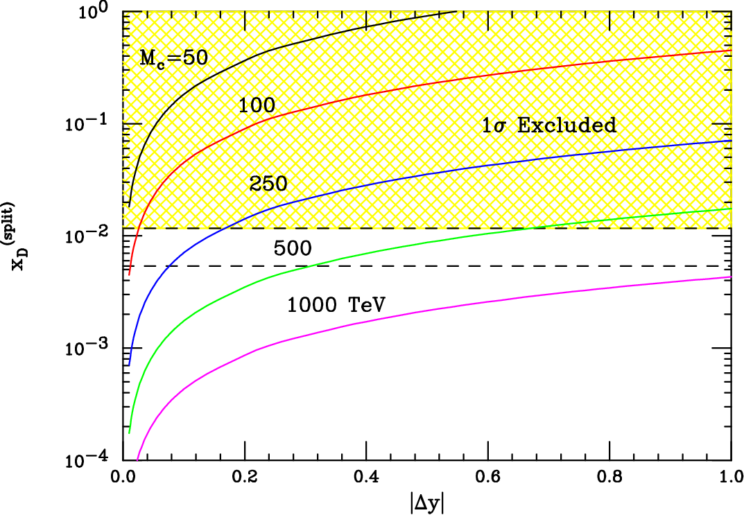
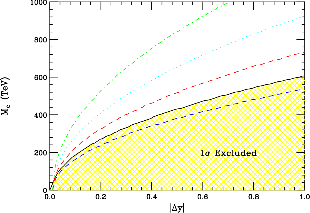
Right: excluded region in the separation and compactification scale parameter plane, as well as possible future contours taking , corresponding to the blue dashed, red dashed, cyan dotted, and green dot-dashed curves, respectively.
Figure 19 shows the range of values for as a function of the separation between the and states for various values of the compactification scale, where . In our numerical work we have used the natural assumption that . We see that vanishes as the separation of the 2 fermions tends to zero as expected. However, for most of the range of , we find that compactification scales of order TeV are excluded by the observation of - mixing and hence mixing provides severe constraints on the localization of the up-type fermions within this model. Note that these constraints are dependent on the choice of values for the elements of the quark diagonalization matrices , which are a priori unknown, and could be reduced if quark mixing is tiny in the up-quark sector. The worst case scenario would be if the are diagonal and all quark mixing occurs in the down-quark sector.99 9 This is frequently the case in models of quark mass matrices where the up-quark mass matrix is taken to be diagonal and all mixing is assigned to the down-quark sector. A rationale for this is given, for example, in Ref. q7. In this case, strong bounds on the compactification scale, similar to those presented here, would be obtained from meson mixing splitfcnc; ben.
VII.3 Warped Geometries
In the simplest scenario with warped extra dimensions rs, known as the Randall-Sundrum (RS) model, the hierarchy between the electroweak and Planck scales is generated geometrically via a large curvature of a single extra dimension. The geometry is that of a 5-dimensional Anti-de-Sitter space (AdS5), where the extent of the dimension is ( is the compactification radius), and every slice of the additional dimension corresponds to a 4-d Minkowski metric. Two 3-branes reside at the boundaries of the AdS5 slice, with the 3-brane located at the fixed point being known as the TeV brane, while the opposite brane at the other boundary is referred to as the Planck brane. Within this framework, gravity is localized about the Planck brane, and electroweak symmetry breaking can take place either with the Higgs field being localized on or near the TeV brane, or via boundary conditions imposed at the fixed points as in the Higgsless models discussed above. The FCNC effects considered here are independent of this choice.
FCNC effects are induced warpfc; soni2 when the SM fermions and gauge bosons are localized in the warped dimension rsgauge; rsfermion; rswall. As in the case of flat TeV-1-sized extra dimensions with split fermions discussed above, the observed fermion masses and mixings are automatically explained by the geometry, with the 5-dimensional Yukawa couplings all being of order unity. Localizing the light fermions near the Planck brane results in small 4-dimensional Yukawa couplings for these fields, whereas if the top-quark field is localized near the TeV brane a large 4-d top Yukawa coupling is induced. This localization scheme also naturally suppresses higher dimensional flavor changing operators that are problematic when the SM is confined to the TeV brane. This flavor breaking fermion localization leads to FCNC interactions via non-universal couplings of the zero-mode fermions to the gauge boson KK states. Since the SM gauge bosons are localized near the TeV brane (in order to acquire their masses) and have exponentially decaying wavefunctions towards the Planck brane, we expect FCNC in the light quark sector to be suppressed.
The action for fermion fields in the RS bulk is given by rsfermion
| (145) |
where represents the determinant of the 5-dimensional metric, is the covariant derivative in curved space, and with being the inverse vierbein. The parameter of importance to us here is which is the 5-dimensional bulk mass for the fermion . It given by , where is the parameter describing the curvature of the AdS5 space and is of order of the 5-d Planck scale. The constants indicate the position of the fermion’s localized wavefunction in the bulk, with corresponding to the fermion being localized near the Planck (TeV) brane. These constants determine the flavor structure of the theory.
The KK decomposition of the bulk fermion fields yields the normalized zero-mode wavefunction (a discrete symmetry ensures that the zero-mode fields are chiral),
| (146) |
| Range of | |
|---|---|
The asymptotic behavior of the on the localization parameters are listed in Table 4. We see that these factors become exponentially small when the fermions are localized near the Planck brane. In the basis where the 5-d bulk masses, , are diagonal the fermion Higgs interactions yield the 4-dimensional Yukawa couplings,
| (147) |
for the zero-mode fermions in terms of the 5-d Yukawa couplings . We take the elements of to be complex and of order unity. Note that in order to resolve the gauge hierarchy problem. The elements of the matrices that diagonalize the up and down quark fields to their 4-d mass eigenstates have magnitude
| (148) |
with for the matrices that diagonalize the right-handed fields. For the elements with one should interchange .
The wavefunctions for the gauge KK states are given by the first order Bessel functions , and the mass of the gauge KK mode is where is related to the roots of Bessel functions rsgauge. The first few values of are 2.45, 5.57, 8.70, and 11.84. Precision electroweak data places severe bounds on the masses of the gauge KK states rsgauge; rsew. However these bounds can be reduced to TeV if the gauge symmetry in the bulk is expanded to , which restores custodial symmetry rscust. The couplings of these states to the zero-mode fermions, , are determined by the overlap of their wavefunctions in the additional dimension. They are given (as a ratio to the SM coupling) by
| (149) |
where is an integral over Bessel functions, and are given explicitly in Ref. rswall and in the Appendix. As displayed in Fig. 20, this coupling weakens substantially as the gauge KK level, , increases for , while for the couplings tend to a small fixed value for all KK levels. The interaction lagrangian for the gluon KK states in the quark mass eigenstate basis is as given in Eq. (139) with the substitution of the prefactor , which arises from the renormalization of the KK gauge kinetic terms to the canonical value.

- mixing is then mediated via tree-level flavor changing interactions of the KK gauge boson states as depicted in Fig. 18. In analogy to the previous section, the effective hamiltonian for this process is given by (for the exchange of gluon KK states which yield the largest contribution)
| (150) |
where . Writing this explicitly for yields,
| (151) |
since the are diagonal, and where the index sums over the generations. Looking at the asymptotic values of in Table 4, we see that is only sizable when the fermion is localized towards the TeV brane. Unitarity of the results in
| (152) |
where is the mass of the first gluon KK excitation, and with the Wilson coefficients being given by
| (153) | |||||
with where are the Bessel function roots described above.
The RG evolution proceeds as in Section II.1 and results in the effective hamiltonian at the charm quark scale
| (154) |
where additional operators have been generated due to mixing in the RG evolution. The evolved Wilson coefficients at the charm scale are as given in Eq. (93) with the appropriate substitution of . Upon evaluating the matrix elements we obtain the contribution to from warped extra dimensions
| (155) |
in the modified vacuum saturation approximation. Here, we have taken the factor of Eq. (67) to be unity.
To obtain numerical results, we need to specify the fermion locations in the warped dimension. We examine three popular scenarios in the literature that correctly generate the 4-d Yukawa hierarchy for the SM fermions. As mentioned above, localizing the fields near the UV (ultraviolet or Planck) brane generates an exponentially small 4-d Yukawa coupling. In all three models, all of the light quarks are localized such that their bulk mass parameters take on values with . Special attention must be paid to the localization of the third generation quarks; in order to generate a large top-quark mass, the corresponding SU(2) singlet field is usually taken to reside close to the TeV brane. The third generation SU(2) doublet fields and -quark SU(2) singlet field are located as close to the IR (infrared, or TeV) brane while maintaining consistency with the experimentally determined coupling. The three scenarios that we follow are fairly uniform in their treatment of the third generation, differing only slightly in the location of the SU(2) top-quark singlet. The scenarios are: (I) A study of flavor physics in the Randall-Sundrum model frankp, (II) A scenario that has been constructed in order to generate fermion masses within the 5-d picture of Higgsless models csakiferm, (III) The up-quark singlet field is taken to lie even closer to the UV brane hooman in order to solve the strong CP problem with warped geometries. The numerical values of the bulk mass parameters are summarized in Table 5 for the three cases.
| Model I | Model II | Model III | |
|---|---|---|---|
| 0.6 | 0.5 | ||
| 0.6 | 1.4 | ||
| 0.52 | 0.5 | ||
| 0.52 | 0.53 | ||
| 0.45 | 0.4 | 0.46 | |
| 0 | 0.3 | on the IR brane |
Our results for for these three models are presented in Fig. 21, where as above, we assume the quark diagonalization matrices take on CKM-like values. In the figure, the dot-dashed green, dashed red, and solid black curves correspond to the bulk mass parameters of Model I, II, and III, respectively. We see from Fig. 20 that fermions localized towards the Planck brane have very small couplings to the KK gluon states and thus do not substantially contribute to . This simplifies the expressions in Eq. (153) in this case, as only the terms have sizable contributions. Looking at the figure we see the mass of the first gluon KK excitation is constrained to lie TeV, which is essentially the same value as the bound obtained from the precision electroweak data in warped models with bulk custodial symmetry rscust. Lastly, we recall from discussion in the previous section, that these constraints can be evaded if the matrix which diagonalizes the up-quark sector is essentially diagonal.

VIII Extra Symmetries
In this section, we focus on supersymmetry. Weak scale supersymmetry is a possible solution to the gauge hierarchy problem, leads to the unification of the gauge couplings at high energies, and provides a natural Dark Matter candidate. It is thus a very well motivated theory of physics beyond the SM. Supersymmetry is an extension of the Poincare symmetry, relating fermions and bosons at a fundamental level. All SM particles have supersymmetric partners (‘sparticles’) with the same mass and gauge interactions, but with spin differing by one-half unit. Since the supersymmetric particles have yet to be discovered, we know that supersymmetry is broken; in this section, we will be agnostic as to which supersymmetry breaking mechanism Nature may have chosen. We note that in non-broken supersymmetry the rates for all loop-induced processes would vanish due to an exact cancellation between the SM and supersymmetric contributions. It is thus due to the breaking of supersymmetry that contributions to FCNC are generated in these theories.
Here, we examine the contributions to - mixing in four supersymmetric scenarios: the Minimal Supersymmetric Standard Model (MSSM), models with alignment in the quark-squark mass matrices, models with R-parity violating couplings, and Split Supersymmetry. Other scenarios with extended non-supersymmetric symmetries have been considered elsewhere in this paper.
VIII.1 Minimal Supersymmetric Standard Model
As the name implies, the MSSM is the simplest version of supersymmetry as it contains the minimal number of new particles. The SM fermions are placed in chiral supermultiplets, the SM gauge bosons lie in vector supermultiplets, and the Higgs sector takes the form of the flavor conserving two-Higgs-doublet Model II discussed above. A discrete symmetry, R-parity, is imposed to forbid unwanted terms in the superpotential that would mediate proton decay at a dangerous level. Conservation of R-parity implies that only pairs of sparticles can be produced or exchanged in loops. Collider searches for direct squark and gluino pair production place the bound GeV PDG in the MSSM with gravity mediated Supersymmetry breaking.
As mentioned above, we will not assume any particular supersymmetry breaking mechanism in our discussion, and so we employ a model independent parameterization of all possible soft supersymmetry breaking terms. This soft supersymmetry breaking sector generally includes three gaugino masses, trilinear scalar interactions, as well as Higgs and sfermion masses, and thus contains many potential sources of flavor violation. Here, we are interested in the flavor violating sources that arise in the up-squark sector. In what is known as the super-CKM basis, the squark fields are rotated by the same matrices that diagonalize the quark masses, giving rise to non-diagonal squark mass matrices. The squark propagators are then expanded such that the non-diagonal mass terms result in mass insertions that change the squark flavor Ellis:1981ts; Nilles:1983ge; Georgi:1986ku; Hall:1985dx. This source of flavor violation differs from that of the SM and many NP models discussed earlier. Here, the quark-squark-gaugino neutral couplings are flavor conserving, while flavor violation arises from the non-diagonality of the squark mass propagators. The mass matrix for the squarks can be divided into sub-matrices,
| (156) |
and the mass insertions can be parameterized in a model independent fashion as
| (157) |
Here, are flavor indices, refers to the helicity choices , , , and represents the average squark mass. Although this source of flavor violation is present in general, and in particular in models with gravity mediated supersymmetry breaking, it can be avoided if supersymmetry is broken by gauge or anomaly mediation. These mass insertions are thought to be small in the MSSM, but can be large in non-minimal supersymmetric models.

In this scenario, the virtual exchange of squarks and gluinos in the box diagrams depicted in Fig. 22 can have a strong contribution to - mixing. Note that the second diagram in the figure is due to the Majorana nature of the gluino. The effective hamiltonian at the supersymmetric scale is given by
| (158) |
where all eight operators in the independent basis contribute. The matching conditions at the supersymmetric mass scale are bigsusyfcnc
| (159) | |||||
where , with being the mass of the gluino. The functions and are given in the Appendix. Note that these conditions are symmetric under the interchange . We also note that the NLO expressions for these matching conditions have been computed in Ref. Ciuchini:2006dw.
The RG evolution to the charm-quark scale results in
| (160) | |||||
which agrees in form with that in Ref. Bagger:1997gg. Here, we have assumed that the squarks and gluinos are integrated out at roughly the same scale. Upon evaluating the matrix elements in the modified vacuum saturation approximation we obtain the MSSM contribution to ,
| (161) | |||||
Here, we have taken the factor of Eq. (67) to be unity.
Our results for are presented in Figs. 23, 24, 25. In these figures, we show contours for the absolute value of the up-charm squark mass insertions for various helicities as a function of the ratio for different average squark masses. These contours correspond to in the three figures. In figure 23, the region above the contours represents the current excluded region. In these figures we take one or two of the mass insertions to be non-vanishing, as indicated. Due to the symmetry of the matching conditions, the constraints on and , as well as and are identical. We see that meson mixing restricts the up and charm squark masses to be degenerate at the level for most of the parameter space. We note that our results numerically agree with those recently computed by Ciuchini et al. Ciuchini:2007cw.


There are several other contributions to meson mixing within the MSSM. These are all mediated via box diagrams with internal sparticle exchange and we now discuss each one in turn. (i) The exchange of any of the 4 neutralinos () with the up and charm squarks. This contribution proceeds via mass insertions in the squark propagators with flavor diagonal quark-squark-neutralino couplings as in the case of internal squark-gluino exchange discussed above. Since the couplings are of weak interaction strength in this case, the magnitude of this contribution is suppressed by the ratio compared to the squark-gluino results and is thus numerically insignificant. (ii) The exchange of one of the neutralinos and one gluino with the up and charm squarks. This again proceeds via the non-diagonal squark mass insertions at a rate of compared to the pure gluino-squark contribution. Although larger than the pure neutralino-squark contribution, it is still a sub-leading effect. (iii) The exchange of charginos () and all three down-type squarks inside the box diagram. Here, the squark propagators are diagonal (mass insertions do not contribute in this case since the internal squarks are ) and the flavor violation is given by the CKM structure of the quark-squark-chargino vertices. However, the squarks are constrained to be highly degenerate from their contributions (with gluino exchange) to meson mixing. Thus a supersymmetric-GIM mechanism is in effect, yielding nearly exact cancellations, and rendering this contribution negligible. This is in contrast to the chargino-squark contributions to meson mixing, where the potentially non-degenerate stop squark participates and can induce large contributions. (iv) The charged Higgs contribution of the two-Higgs-Doublet model of type II discussed in Section VI.1. As shown in that section, these contributions are numerically small, even in the case of large . In summary, we see that all other supersymmetric contributions to - mixing are numerically insignificant compared to the squark-gluino exchange. It is interesting to note that stop-squarks do not contribute to meson mixing.
VIII.2 Quark-Squark Alignment Models
As we saw in the previous Section, in the MSSM there is a new “flavor problem,” namely, how to keep the contributions from the supersymmetric particles to FCNC as small as the observations. The conventional solution is to impose constraints, such as those derived above, of (i) degeneracy in the squark sector (except for the special case of stop squarks), i.e. the diagonal sub-matrices and in Eq. (157) should be proportional to the unit matrix, and (ii) the non-diagonal sub-matrices should be proportional to the corresponding quark matrix.
Nir and Seiberg Nir:1993mx have proposed an alternative to this picture where the quark and squark mass matrices are approximately aligned with each other. Their proposal is as follows: if for some symmetry reason the matrices corresponding to the squark mass insertions, , are themselves diagonal, then the squark contributions to FCNC vanish, regardless of the mass spectrum of the squarks. Corrections to this approximation are expected to remain tolerably small and it should be possible to simultaneously diagonalize the quark mass matrices and the squark mass-squared matrices while essentially preserving flavor diagonal gluino interactions.
Within this framework, it is somewhat problematic to satisfy the constraints from - mixing. Specific implementations of this proposal, based on Abelian horizontal symmetries, restrict the supersymmetric contributions to Kaon mixing via a unique structure for the down quark mass matrix using holomorphic zeros Nir:2002ah. This implies that Cabibbo mixing between the first and second generation quarks must be induced by mixing in the up-quark sector, which in turn leads to sizable supersymmetric contributions to - mixing. In this case, mixing in the up-charm squark sector gives
| (162) |
where is the Cabibbo angle, while the mass insertions can naturally remain small. Mirroring the above discussion for MSSM, this leads to the effective Hamiltonian that mediates mixing
| (163) |
with
| (164) |
where with are again given in the Appendix. The RG evolution is simple and yields
| (165) |
The bounds on from the current measurement of meson mixing are given in the upper left-hand panel of Fig. 23. Using Eq. (162) above, this results in the constraint on squark and gluino masses of (assuming for simplicity) TeV, which agrees with the results in Refs. Nir:2007ac; Ciuchini:2007cw. This would exclude early discovery of Supersymmetry at the LHC, but leaves a discovery window with higher luminosities as the LHC detectors are expected to have a search reach of up to TeV with 300 fb-1 of integrated luminosity.
VIII.3 Supersymmetry with R-Parity Violation
The conventional gauge symmetries of supersymmetry allow for the existence of additional terms in the superpotential that violate baryon and lepton number. The assumption of R-parity conservation in the MSSM prohibits these terms, ensuring that baryon and lepton number are conserved, and forbids related dangerous operators, e.g., those that mediate proton decay. However, it is possible to construct alternative discrete symmetries Ibanez:1991pr, such as baryon-parity or lepton-parity, that allow terms which violate either baryon or lepton number, but not both. These symmetries also forbid unwanted operators, and there is no strong theoretical motivation to prefer R-parity over these alternative scenarios. The R-parity violating terms in the superpotential can be written as
| (166) |
are generation indices and symmetry demands () in the terms proportional to (). The quantities in Eq. (166) are the chiral superfields in the MSSM, and the , indices have been suppressed. A bilinear term may also be present, but it can be rotated away and will not be considered here. The lepton number violating terms, and , cannot exist simultaneously with the term containing . The terms have the same structure as the couplings for scalar leptoquarks, as discussed in Section VI.3. This model still contains the minimal superfield content, but leads to a markedly different supersymmetric phenomenology as sparticles can now be produced singly and can mediate FCNC at tree-level.
The superfields are in the weak basis and should be rotated to their mass eigenstates. The term becomes Agashe:1995qm
| (167) |
with the definition
| (168) |
Here, and are the matrices which rotate the left-handed up- and right-handed down-quark fields to their mass basis. Written in terms of component fields, the second term in this superpotential contains the interactions
| (169) | |||||
where the second line involving the up-quark sector is relevant for - mixing.
Constraints on the size of these R-parity violating couplings have been obtained in the literature. These limits are derived from considerations of various processes Allanach:1999ic such as charged current universality, semi-leptonic meson decays, rare meson decays, atomic parity violation, double nucleon decay, neutron oscillations, and boson decays. A compilation of the bounds on the couplings relevant for - mixing are given in Table 6. In addition, the recently improved upper bound on the branching fraction for the process of from CLEO-c He:2005iz yields the stringent restriction Burdman:2001tf on the product of couplings .
It is possible for the quark flavor rotations to generate flavor violation in the down- or up-quark sectors, but not both. In the case where the flavor rotations occur in the up-quark sector only, large flavor changing effects are expected in the meson system and the limits on the R-parity violating couplings shown in Table 6 become modified Allanach:1999ic. However, this scenario is rather model dependent, we will adopt a more conservative, model-independent formalism in the following.
| 0.043 | 0.11 | 0.52 | |||
| 1.23 | 1.23 | 1.23 |
For the lepton number violating coupling , the first and third terms in the second line of Eq. (128) mediate - mixing via box diagrams where either the pair or are exchanged internally with the assignment of the generational index Agashe:1995qm. The corresponding Feyman diagrams are depicted in Fig. 26. Note that there are no tree-level contributions as in the case of meson mixing in the down-quark sector. This is described at the high mass scale by the effective hamiltonian
| (170) |
where the dependence on the operator is induced due to the fermion propagator. This interaction will yield constraints on the product of couplings . Here, we have assumed that only one set of the R-parity violating couplings (i.e., only one value of and ) is large and dominant. This is equivalent to saying that, e.g., both sleptons and both down-type quarks being exchanged in the first box diagram shown in Fig. 26 are from the same generation. In general, this need not be the case and, for example, the coupling factor would then be the product , with, e.g., the set of being exchanged.

Matching at the SUSY scale yields the Wilson coefficient
| (171) |
Computing the evolution to the charm-quark scale yields
| (172) |
with
| (173) |
Evaluating the appropriate matrix element gives the mixing contribution for the R-parity violating terms,
| (174) |
Taking for simplicity, we obtain the constraint
| (175) |
which yields numerically
| (176) |
We find that relaxing our assumption on the slepton mass and taking strengthens this bound at most by a factor of 3.7 when GeV. In computing the RGE evolution we used the value GeV and find little sensitivity in the evolution on the squark mass once it is above the current experimental limit from HERA of GeV PDG. It is trivial to scale our result in Eq. (176) to compare to the limits in Table 6 which are based on setting GeV. Taking, GeV, we see that the bounds on from - mixing are a factor of 50 (250) times stronger than those in the Table for ().
The full numerical results for and the constraints obtained in the R-parity violating coupling, squark mass parameter plane are presented in Fig. 27 in the limit . We see that meson mixing provides stringent constraints on R-parity violating couplings. These bounds can be directly translated to constraints on the couplings of scalar leptoquarks as discussed in a previous Section.


The baryon number violating couplings can also contribute to - mixing. We remind the reader that they cannot exist simultaneously with the lepton number violating terms in the superpotential. They participate in mixing via -quark and exchange in the box diagram. The formalism is analogous to the case above. The effective hamiltonian at the SUSY mass scale is
| (177) |
Recall that symmetry dictates . After completing the RGE evolution as described above, and assuming the charged squarks are degenerate, we have
| (178) |
This yields the constraint
| (179) |
which mirrors that for the lepton number violating scenario.
VIII.4 Split Supersymmetry
Lastly, for completeness, we briefly discuss the case of Split Supersymmetry nimagian. This scenario postulates that supersymmetry breaking occurs at a very high scale, TeV. The scalar particles all acquire masses at this high scale, except for a single neutral Higgs boson, whose mass is either finely-tuned or is preserved by some other mechanism. Split Supersymmetry proponents argue that this tuning may, indeed, be present in Nature, perhaps being related to the cosmological constant problem (which suffers an even greater degree of fine-tuning). The fermions in this theory, including the gauginos, are assumed to be protected by chiral symmetries and thus can have weak-scale masses. This feature preserves the gauge coupling unification found in supersymmetric models, and provides a natural Dark Matter candidate in the lightest neutralino. One important consequence of this scenario is that since all the scalar fields are present at only a very high scale, they decouple from physics at the TeV scale and their contributions to FCNC in the flavor sector are negligible. Since all contributions to - mixing in supersymmetry involve the internal exchange of scalar quarks, we expect these effects to essentially vanish in this scenario.
IX Conclusions
The recent BaBar and Belle findings on - mixing have brought the long standing search for this phenomenon to a successful conclusion, although much remains to be done. Compared to mixing in the other flavor sectors, the observed value for charm (cf Eq. (4)) is by far the smallest,
| (180) |
In our opinion, the measured value for is in accord with expectations of the Standard Model, with the proviso that hadronic (rather than quark-level) effects are the dominating influence (cf Sect. III). We have argued that the relatively small magnitude of charm mixing could afford New Physics an enhanced chance to compete successfully with the Standard Model. It should be kept in mind, however, that the current experimental value of is relatively imprecise and that the SM theoretical determination contains hadronic uncertainties. These facts tend to frustrate the attempt to disentangle any potentially large NP contribution from that of the SM.
By design, our study of NP contributions has addressed a rather broad spectrum of possibilities. We have avoided playing favorites among the NP models contained in this paper, letting the results speak for themselves. Since the average reader is unlikely to be conversant with the details of such a large array of NP models, our presentation has been pedagogical in nature. We have tried to precede any formula for with a summary of the relevant background.
A work such as this is meant to constrain the parameter spaces of NP models. The case of mixing is especially interesting because the intermediate states which generate the -to- transitions are distinct from those occurring in , and mixing. Typically, NP parameters will involve the masses of yet-to-be-discovered particles and their coupling strengths to ordinary matter. In some cases (Left-Right Symmetric Model, Split Supersymmetry, Universal Extra Dimensions, Flavor Conserving Two-Higgs Doublets) we have found that the NP model will not generate a - signal at the observed level for any values of its parameters. More often, however, this is not the case and for some models (Split Fermions, Flavor Changing Neutral Higgs) the constraints can be strong.
The main quantitative conclusions for this work appear in the set of figures which appear throughout the paper. For convenience, we have compiled a summary of our results in Table 7, using the value to mark the boundary between allowed and excluded regions. Such a list is by nature approximate, and we refer the reader to the body of the paper for a more precise presentation of our results.
| Model | Approximate Constraint |
|---|---|
| Fourth Generation (Fig. 2) | (GeV) |
| Singlet Quark (Fig. 4) | (GeV) |
| Singlet Quark (Fig. 6) | |
| Little Higgs | Tree: See entry for Singlet Quark |
| Box: Region of parameter space can reach observed | |
| Generic (Fig. 7) | TeV |
| Family Symmetries (Fig. 8) | TeV (with ) |
| Left-Right Symmetric (Fig. 9) | No constraint |
| Alternate Left-Right Symmetric (Fig. 10) | TeV ( TeV) |
| ( TeV-1 | |
| Vector Leptoquark Bosons (Fig. 11) | TeV |
| Flavor Conserving Two-Higgs-Doublet (Fig. 13) | No constraint |
| Flavor Changing Neutral Higgs (Fig. 15) | TeV |
| FC Neutral Higgs (Cheng-Sher ansatz) (Fig. 16) | GeV |
| Scalar Leptoquark Bosons | See entry for RPV SUSY |
| Higgsless (Fig. 17) | TeV |
| Universal Extra Dimensions | No constraint |
| Split Fermion (Fig. 19) | |
| Warped Geometries (Fig. 21) | TeV |
| Minimal Supersymmetric Standard (Fig. 23) | for TeV |
| for TeV | |
| Supersymmetric Alignment | TeV |
| Supersymmetry with RPV (Fig. 27) | GeV |
| Split Supersymmetry | No constraint |
We recommend further experimental study of this subject on two fronts. First, of course, is the need to reduce error bars in the measured values of and especially . Equally important is continuing the search for evidence of CP violation in mixing for the system. CP violation provides an interesting contrast with mixing because it provides an independent arena for competition between the SM and NP signals. There is especially room for improvement in the SM analysis of charm CP violation, and work on this is underway.
Acknowledgements.
The work of E.G. was supported in part by the U.S. National Science Foundation under Grant PHY–0555304, J.H. was supported by the U.S. Department of Energy under Contract DE-AC02-76SF00515, S.P. was supported by the U.S. Department of Energy under Contract DE-FG02-04ER41291 and A.P. was supported in part by the U.S. National Science Foundation under CAREER Award PHY–0547794, and by the U.S. Department of Energy under Contract DE-FG02-96ER41005. J.H. would like to thank the theoretical physics group at Fermilab for their hospitality and E.G., J.H., and A.P. thank the High Energy Physics Group at the University of Hawaii for their hospitality while part of this work was performed. We would like to thank C.F. Berger, S. Chivukula, B. Dobrescu, J. Donoghue, K.C. Kong, B. Lillie, E. Lunghi, E. Simmons and T. Tait for discussions related to this work and especially T. Browder, T. Rizzo, and X. Tata for a careful reading of the manuscript.Appendix A Collected Formulae
Here, we collect the formulae used throughout the manuscript to compute the contributions to - mixing in the various New Physics models.
Inami-Lim: (from Ref. Inami:1980fz)
The loop functions, first calculated by Inami Lim, apply for several NP scenarios discussed in the text. For a contribution from two internal quarks of the same flavor in the box diagram, the loop function is
| (181) |
and for two quarks of different flavors,
| (182) |
Little Higgs: (from Ref. Hubisz:2005bd)
The loop function for the case where the mirror fermions and heavy gauge bosons are exchanged in the box diagram is given by
| (183) | |||||
with
| (184) |
Left-Right Symmetric Model:
The loop function with one and one boson being exchanged in the box diagram is
| (185) |
Charged Higgs: (from Ref. bhp)
The loop functions with one and one SM boson and with two being exchanged in the box diagram are
| (186) | |||||
Cheng-Sher box:
The loop function in the Cheng-Sher ansatz with flavor changing neutral Higgs bosons for a top quark and neutral Higgs being exchanged in a box diagram is
| (187) |
Universal Extra Dimensions:
The expressions for the case of Universal Extra Dimenions are given in full in Ref. Buras:2002ej.
Warped Extra Dimensions: (from Ref. rswall)
The coupling of two zero-mode fermions to the gauge boson KK state, , relative to the SM coupling strength is
| (188) |
where the roots for the gauge boson KK spectrum are given by
| (189) |
and is defined by
| (190) |
Supersymmetry: (from Ref. bigsusyfcnc)
The loop functions from squark and gluino exchange in a box diagram with squark mass insertions are given by
| (191) |
References
- (1)
- (2) A. Datta and D. Kumbhakar, Z. Phys. C 27, 515 (1985).
- (3) The BaBaR Collaboration, B. Aubert, et al., ’Evidence for - Mixing’, arXiv:hep-ex/0703020.
- (4) Belle Collaboration: M. Staric, et al., ’Evidence for - Mixing’, arXiv:hep-ex/0703036.
- (5) Belle Collaboration: K. Abe, et al., ’Measurement of - mixing in decays’, arXiv:hep-ex/0704.1000.
- (6) The BaBar Collaboration, B. Aubert, et al., ‘Search for mixing using doubly flavor tagged semileptonic decay modes,’ arXiv:0705.0704 [hep-ex].
- (7) G. Burdman and I. Shipsey, Ann. Rev. Nucl. Part. Sci. 53, 431 (2003) [arXiv:hep-ph/0310076]; G. Burdman, E. Golowich, J.L. Hewett and S. Pakvasa, Phys. Rev. D 52, 6383 (1995) [arXiv:hep-ph/9502329]; J.L. Hewett, T. Takeuchi and S.D. Thomas, in Electroweak Symmetry Breaking and Beyond the Standard Model ed. by T. Barklow, et al., World Scientific, arXiv:hep-ph/9603391; S. Bianco, F. L. Fabbri, D. Benson and I. Bigi, Riv. Nuovo Cim. 26N7, 1 (2003) [arXiv:hep-ex/0309021]; A. A. Petrov, Int. J. Mod. Phys. A 21, 5686 (2006) [arXiv:hep-ph/0611361]; A. A. Petrov, In the Proceedings of Flavor Physics and CP Violation (FPCP 2003), Paris, France, 3-6 Jun 2003, pp MEC05 [arXiv:hep-ph/0311371]; H. N. Nelson, in Proc. of the 19th Intl. Symp. on Photon and Lepton Interactions at High Energy LP99 ed. J.A. Jaros and M.E. Peskin, arXiv:hep-ex/9908021.
- (8) G. Burdman, E. Golowich, J. Hewett and S. Pakvasa, Phys. Rev. D 66, 014009 (2002) [arXiv:hep-ph/0112235].
- (9) Heavy Flavor Averaging Group, http://www.slac.stanford.edu/xorg/hfag/charm/index.html; D. Asner, ‘Charm Physics’, talk at the Workshop on Flavor in the Era of the LHC, CERN (3/26-28/07); B. Peterson, talk given at the Charm 2007 Workshop, Cornell University, Ithaca, NY, August 2007.
- (10) E. Golowich and A.A. Petrov, Phys. Lett. B 625, 53 (2005) [arXiv:hep-ph/0506185].
- (11) A. F. Falk, Y. Nir and A. A. Petrov, JHEP 9912, 019 (1999) [arXiv:hep-ph/9911369].
- (12) S. Bergmann, Y. Grossman, Z. Ligeti, Y. Nir and A.A. Petrov, Phys. Lett. B 486, 418 (2000) [arXiv:hep-ph/0005181].
- (13) Y. Nir, ‘Lessons from BaBar and Belle measurements of mixing parameters,’ arXiv:hep-ph/0703235.
- (14) Particle Data Group (W.-M. Yao et al.), ‘Review of Particle Physics’, J.Phys.G33:1-1232,2006.
- (15) E. Golowich, S. Pakvasa and A.A. Petrov, Phys. Rev. Lett. 98, 181808-1 (2007) [arXiv:hep-ph/0610039].
- (16) M. Ciuchini, E. Franco, V. Lubicz, G. Martinelli, I. Scimemi and L. Silvestrini, Nucl. Phys. B 523, 501 (1998) [arXiv:hep-ph/9711402].
- (17) R. Gupta, T. Bhattacharya and S. R. Sharpe, Phys. Rev. D 55, 4036 (1997) [arXiv:hep-lat/9611023].
- (18) M. Artuso et al. [CLEO Collaboration], Phys. Rev. Lett. 95, 251801 (2005) [arXiv:hep-ex/0508057].
- (19) A.A. Petrov, Phys. Rev. D 56, 1685 (1997) [arXiv:hep-ph/9703335]; H. Georgi, Phys. Lett. B297, 353 (1992); T. Ohl et al., Nucl. Phys. B403, 605 (1993).
- (20) I.I.Y. Bigi and N.G. Uraltsev, Nucl. Phys. B 592, 92 (2001) [arXiv:hep-ph/0005089].
- (21) A.F. Falk, Y. Grossman, Z. Ligeti and A.A. Petrov, Phys. Rev. D 65, 054034 (2002) [arXiv:hep-ph/0110317].
- (22) E. Golowich, A.A. Petrov and G. Yeghiyan (in progress).
- (23) E. Golowich and A. A. Petrov, Phys. Lett. B 427, 172 (1998) [arXiv:hep-ph/9802291].
- (24) J.F. Donoghue, E. Golowich, B.R. Holstein and J. Trampetic, Phys. Rev. D 33, 179 (1986).
- (25) L. Wolfenstein, Phys. Lett. B164, 170 (1985).
- (26) F. Buccella, M. Lusignoli, G. Miele, A. Pugliese and P. Santorelli, Phys. Rev. D 51, 3478 (1995) [arXiv:hep-ph/9411286].
- (27) A.F. Falk, Y. Grossman, Z. Ligeti, Y. Nir and A.A. Petrov, Phys. Rev. D 69, 114021 (2004) [arXiv:hep-ph/0402204].
- (28) M.E. Peskin and T. Takeuchi, Phys. Rev. D 46, 381 (1992).
- (29) LEP Electroweak Working Group, Phys. Rept. 427, 257 (2006) [arXiv:hep-ex/0509008].
- (30) See, for example, H.J. He, N. Polonsky and S.F. Su, Phys. Rev. D 64, 053004 (2001) [arXiv:hep-ph/0102144].
- (31) M.S. Chanowitz, M.A. Furman and I. Hinchliffe, Phys. Lett. B 78, 285 (1978); Nucl. Phys. B 153, 402 (1979).
- (32) K.S. Babu, X.G. He, X. Li and S. Pakvasa, Phys. Lett. B 205, 540 (1988).
- (33) T. Inami and C.S. Lim, Prog. Theor. Phys. 65, 297 (1981) [Erratum-ibid. 65, 1772 (1981)].
- (34) G.C. Branco, P.A. Parada and M.N. Rebelo, Phys. Rev. D 52, 4217 (1995) [arXiv:hep-ph/9501347].
- (35) F. Gursey, P. Ramond and P. Sikivie, Phys. Lett. B 60, 177 (1976).
- (36) J.L. Hewett and T.G. Rizzo, Phys. Rept. 183, 193 (1989).
- (37) N. Arkani-Hamed, A.G. Cohen, E. Katz and A.E. Nelson, JHEP 0207, 034 (2002) [arXiv:hep-ph/0206021].
- (38) N. Arkani-Hamed, A.G. Cohen, E. Katz, A.E. Nelson, T. Gregoire and J.G. Wacker, JHEP 0208, 021 (2002) [arXiv:hep-ph/0206020].
- (39) J.D. Bjorken, S. Pakvasa and S.F. Tuan, Phys. Rev. D 66, 053008 (2002) [arXiv:hep-ph/0206116].
- (40) S.L. Glashow and S. Weinberg, Phys. Rev. D 15, 1958 (1977); E. Paschos, Phys. Rev. D 15, 1966 (1977).
- (41) N. Arkani-Hamed, A.G. Cohen and H. Georgi, Phys. Lett. B 513, 232 (2001) [arXiv:hep-ph/0105239]; For a review, see, M. Perelstein, Prog. Part. Nucl. Phys. 58, 247 (2007) [arXiv:hep-ph/0512128].
- (42) J. Y. Lee, JHEP 0412, 065 (2004) [arXiv:hep-ph/0408362].
- (43) C. H. Chen, C. Q. Geng and T. C. Yuan, ‘- mixing and rare D decays in the Littlest Higgs model with non-unitarity matrix,’ arXiv:0704.0601 [hep-ph].
- (44) C. Csaki, J. Hubisz, G. D. Kribs, P. Meade and J. Terning, Phys. Rev. D 67, 115002 (2003) [arXiv:hep-ph/0211124]; J. L. Hewett, F. J. Petriello and T. G. Rizzo, JHEP 0310, 062 (2003) [arXiv:hep-ph/0211218]; M. C. Chen and S. Dawson, Phys. Rev. D 70, 015003 (2004) [arXiv:hep-ph/0311032].
- (45) C. Csaki, J. Hubisz, G. D. Kribs, P. Meade and J. Terning, Phys. Rev. D 68, 035009 (2003) [arXiv:hep-ph/0303236].
- (46) H. C. Cheng and I. Low, JHEP 0309, 051 (2003) [arXiv:hep-ph/0308199]; H. C. Cheng and I. Low, JHEP 0408, 061 (2004) [arXiv:hep-ph/0405243].
- (47) C. T. Hill and R. J. Hill, arXiv:hep-ph/0701044; C. T. Hill and R. J. Hill, arXiv:0705.0697 [hep-ph].
- (48) J. Hubisz, S. J. Lee and G. Paz, JHEP 0606, 041 (2006) [arXiv:hep-ph/0512169]; M. Blanke, A. J. Buras, A. Poschenrieder, C. Tarantino, S. Uhlig and A. Weiler, JHEP 0612, 003 (2006) [arXiv:hep-ph/0605214].
- (49) M. Blanke, A. J. Buras, S. Recksiegel, C. Tarantino and S. Uhlig, ‘Littlest Higgs model with T-parity confronting the new data on mixing,’ arXiv:hep-ph/0703254.
- (50) See, for example, P. Savard, “Searches for Extra Dimensions and New Gauge Bosons at the Tevatron,” talk given at the XXXIII International Conference on High Energy Physics, 26 July-2 August 2006, Moscow, Russia; T. Adams, “Searches for New Phenomena with Lepton Final States at the Tevatron,” talk given at Rencontres de Moriond Electroweak Interactions and Unified Theories 2007, La Thuile, Italy 10-17 March 2007; A. Abulencia et al. [CDF Collaboration], ‘Search for boson decaying to electron-neutrino pairs in collisions at TeV,’ arXiv:hep-ex/0611022.
- (51) T. G. Rizzo, ’Z’ phenomenology and the LHC’, arXiv:hep-ph/0610104.
- (52) P. Langacker and M. Plumacher, Phys. Rev. D 62, 013006 (2000) [arXiv:hep-ph/0001204].
- (53) A. Arhrib, K. Cheung, C. W. Chiang and T. C. Yuan, Phys. Rev. D 73, 075015 (2006) [arXiv:hep-ph/0602175].
- (54) X-G He and G. Valencia, ‘ mixing constraints on FCNC with a non-universal ’, arXiv:hep-ph/0703270.
- (55) F. Wilczek and A. Zee, Phys. Rev. Lett. 42, 421 (1979).
- (56) V. A. Monich, B. V. Struminsky and G. G. Volkov, Phys. Lett. B 104, 382 (1981) [JETP Lett. 34, 213.1981 ZETFA,34,222 (1981 ZETFA,34,222-225.1981)].
- (57) R. N. Mohapatra and J. C. Pati, Phys. Rev. D 11, 2558 (1975). For a review and complete set of original references, see R.N. Mohapatra, Unification and Supersymemtry, (Springer, New York, 1986).
- (58) N. G. Deshpande, E. Keith and T. G. Rizzo, Phys. Rev. Lett. 70, 3189 (1993) [arXiv:hep-ph/9211310].
- (59) K. Kiers, M. Assis and A. A. Petrov, Phys. Rev. D 71, 115015 (2005) [arXiv:hep-ph/0503115].
- (60) G. Beall, M. Bander and A. Soni, Phys. Rev. Lett. 48, 848 (1982).
- (61) D. Chang, R. N. Mohapatra and M. K. Parida, Phys. Rev. D 30, 1052 (1984).
- (62) F. I. Olness and M. E. Ebel, Phys. Rev. D 30, 1034 (1984); P. Langacker and S. Uma Sankar, Phys. Rev. D 40, 1569 (1989).
- (63) T. G. Rizzo, Phys. Rev. D 50, 325 (1994) [arXiv:hep-ph/9311265].
- (64) Z. Chacko, H. S. Goh and R. Harnik, Phys. Rev. Lett. 96, 231802 (2006) [arXiv:hep-ph/0506256]; H. S. Goh and S. Su, Phys. Rev. D 75, 075010 (2007) [arXiv:hep-ph/0611015].
- (65) K. S. Babu, X. G. He and E. Ma, Phys. Rev. D 36, 878 (1987).
- (66) E. Ma, Mod. Phys. Lett. A 3, 319 (1988).
- (67) W. Buchmuller, R. Ruckl and D. Wyler, Phys. Lett. B 191, 442 (1987) [Erratum-ibid. B 448, 320 (1999)].
- (68) G. G. Ross, Grand Unified Theories, Benjamin/Cummings Pub. Co., Menlo Park, CA (1984).
- (69) B. Abbott et al. [D0 Collaboration], Phys. Rev. Lett. 83, 2896 (1999) [arXiv:hep-ex/9904023].
- (70) S. Davidson, D. C. Bailey and B. A. Campbell, Z. Phys. C 61, 613 (1994) [arXiv:hep-ph/9309310].
- (71) M. Leurer, Phys. Rev. D 50, 536 (1994) [arXiv:hep-ph/9312341].
- (72) For a summary, see, J. L. Hewett and T. G. Rizzo, Phys. Rev. D 56, 5709 (1997) [arXiv:hep-ph/9703337].
- (73) See, for example, B. Grinstein and M. B. Wise, Phys. Lett. B 201, 274 (1988); T. G. Rizzo, Phys. Rev. D 38, 820 (1988); J.L. Hewett, Phys. Rev. Lett. 70, 1045 (1993) [arXiv:hep-ph/9211256]; V.D. Barger, M. S. Berger and R. J. N. Phillips, Phys. Rev. Lett. 70, 1368 (1993) [arXiv:hep-ph/9211260].
- (74) M. Misiak et al., Phys. Rev. Lett. 98, 022002 (2007) [arXiv:hep-ph/0609232].
- (75) V.D. Barger, J.L. Hewett and R.J.N. Phillips, Phys. Rev. D 41, 3421 (1990).
- (76) G. Isidori and A. Retico, JHEP 0111, 001 (2001) [arXiv:hep-ph/0110121]; A.J. Buras, P.H. Chankowski, J. Rosiek and L. Slawianowska, Nucl. Phys. B 619, 434 (2001) [arXiv:hep-ph/0107048].
- (77) S. Pakvasa and H. Sugawara, Phys. Lett. 73B, 61 (1978.)
- (78) T.P. Cheng and M. Sher, Phys. Rev. D 35, 3484 (1987).
- (79) L. J. Hall and S. Weinberg, Phys. Rev. D 48, 979 (1993) [arXiv:hep-ph/9303241].
- (80) D. Acosta et al. [CDF Collaboration], Phys. Rev. D 72, 051107 (2005) [arXiv:hep-ex/0506074]; A. Abulencia et al. [CDF Collaboration], Phys. Rev. D 73, 051102 (2006) [arXiv:hep-ex/0512055].
- (81) R. S. Chivukula, N. J. Evans and E. H. Simmons, Phys. Rev. D 66, 035008 (2002) [arXiv:hep-ph/0204193].
- (82) N. Arkani-Hamed, A. G. Cohen, T. Gregoire and J. G. Wacker, JHEP 0208, 020 (2002) [arXiv:hep-ph/0202089].
- (83) C. Csaki, C. Grojean, L. Pilo and J. Terning, Phys. Rev. Lett. 92, 101802 (2004) [arXiv:hep-ph/0308038].
- (84) C. Csaki, C. Grojean, H. Murayama, L. Pilo and J. Terning, Phys. Rev. D 69, 055006 (2004) [arXiv:hep-ph/0305237].
- (85) Y. Nomura, JHEP 0311, 050 (2003) [arXiv:hep-ph/0309189]; R. Barbieri, A. Pomarol and R. Rattazzi, Phys. Lett. B 591, 141 (2004) [arXiv:hep-ph/0310285]; H. Davoudiasl, J. L. Hewett, B. Lillie and T. G. Rizzo, Phys. Rev. D 70, 015006 (2004) [arXiv:hep-ph/0312193]; G. Burdman and Y. Nomura, Phys. Rev. D 69, 115013 (2004) [arXiv:hep-ph/0312247]; G. Cacciapaglia, C. Csaki, C. Grojean and J. Terning, Phys. Rev. D 70, 075014 (2004) [arXiv:hep-ph/0401160]; H. Davoudiasl, J. L. Hewett, B. Lillie and T. G. Rizzo, JHEP 0405, 015 (2004) [arXiv:hep-ph/0403300].
- (86) C. Csaki, C. Grojean, J. Hubisz, Y. Shirman and J. Terning, Phys. Rev. D 70, 015012 (2004) [arXiv:hep-ph/0310355].
- (87) For a review of TeV-scale extra dimensional models and their experimental consequences, see for example, J. Hewett and M. Spiropulu, Ann. Rev. Nucl. Part. Sci. 52, 397 (2002) [arXiv:hep-ph/0205106]; T. G. Rizzo, In the Proceedings of 32nd SLAC Summer Institute on Particle Physics (SSI 2004): Natures Greatest Puzzles, Menlo Park, California, 2-13 Aug 2004, pp L013 [arXiv:hep-ph/0409309].
- (88) I. Antoniadis, Phys. Lett. B 246, 377 (1990); J. D. Lykken, Phys. Rev. D 54, 3693 (1996) [arXiv:hep-th/9603133]; I. Antoniadis and M. Quiros, Phys. Lett. B 392, 61 (1997) [arXiv:hep-th/9609209].
- (89) T. Appelquist, H. C. Cheng and B. A. Dobrescu, Phys. Rev. D 64, 035002 (2001) [arXiv:hep-ph/0012100].
- (90) G. Servant and T. M. P. Tait, Nucl. Phys. B 650, 391 (2003) [arXiv:hep-ph/0206071], New J. Phys. 4, 99 (2002) [arXiv:hep-ph/0209262]; H. C. Cheng, J. L. Feng and K. T. Matchev, Phys. Rev. Lett. 89, 211301 (2002) [arXiv:hep-ph/0207125].
- (91) C. Lin, ’Search for Universal Extra Dimensions in the Multi-Lepton Channel at the Tevatron’, CDF Thesis, FERMILAB-PUB-05-572-E.
- (92) H. C. Cheng, K. T. Matchev and M. Schmaltz, Phys. Rev. D 66, 036005 (2002) [arXiv:hep-ph/0204342].
- (93) A. J. Buras, M. Spranger and A. Weiler, Nucl. Phys. B 660, 225 (2003) [arXiv:hep-ph/0212143].
- (94) N. Arkani-Hamed, Y. Grossman and M. Schmaltz, Phys. Rev. D 61, 115004 (2000) [arXiv:hep-ph/9909411].
- (95) E. A. Mirabelli and M. Schmaltz, Phys. Rev. D 61, 113011 (2000) [arXiv:hep-ph/9912265]; G. C. Branco, A. de Gouvea and M. N. Rebelo, Phys. Lett. B 506, 115 (2001) [arXiv:hep-ph/0012289]; D. E. Kaplan and T. M. P. Tait, JHEP 0111, 051 (2001) [arXiv:hep-ph/0110126]; Y. Grossman and G. Perez, Phys. Rev. D 67, 015011 (2003) [arXiv:hep-ph/0210053]; C. Biggio, F. Feruglio, I. Masina and M. Perez-Victoria, Nucl. Phys. B 677, 451 (2004) [arXiv:hep-ph/0305129]; B. Lillie, JHEP 0312, 030 (2003) [arXiv:hep-ph/0308091]; Y. Grossman, R. Harnik, G. Perez, M. D. Schwartz and Z. Surujon, Phys. Rev. D 71, 056007 (2005) [arXiv:hep-ph/0407260]; G. Perez and T. Volansky, Phys. Rev. D 72, 103522 (2005) [arXiv:hep-ph/0505222].
- (96) A. Delgado, A. Pomarol and M. Quiros, JHEP 0001, 030 (2000) [arXiv:hep-ph/9911252]; W. F. Chang and J. N. Ng, JHEP 0212, 077 (2002) [arXiv:hep-ph/0210414].
- (97) B. Lillie and J. L. Hewett, Phys. Rev. D 68, 116002 (2003) [arXiv:hep-ph/0306193].
- (98) L. Randall and R. Sundrum, Phys. Rev. Lett. 83, 3370 (1999) [arXiv:hep-ph/9905221].
- (99) S. J. Huber and Q. Shafi, Phys. Lett. B 498, 256 (2001) [arXiv:hep-ph/0010195]; S. J. Huber, Nucl. Phys. B 666, 269 (2003) [arXiv:hep-ph/0303183]; G. Burdman, Phys. Lett. B 590, 86 (2004) [arXiv:hep-ph/0310144]; K. Agashe, G. Perez and A. Soni, Phys. Rev. Lett. 93, 201804 (2004) [arXiv:hep-ph/0406101].
- (100) K. Agashe, G. Perez and A. Soni, Phys. Rev. D 71, 016002 (2005) [arXiv:hep-ph/0408134].
- (101) H. Davoudiasl, J. L. Hewett and T. G. Rizzo, Phys. Lett. B 473, 43 (2000) [arXiv:hep-ph/9911262]; A. Pomarol, Phys. Lett. B 486, 153 (2000) [arXiv:hep-ph/9911294].
- (102) Y. Grossman and M. Neubert, Phys. Lett. B 474, 361 (2000) [arXiv:hep-ph/9912408]; T. Gherghetta and A. Pomarol, Nucl. Phys. B 586, 141 (2000) [arXiv:hep-ph/0003129].
- (103) H. Davoudiasl, J. L. Hewett and T. G. Rizzo, Phys. Rev. D 63, 075004 (2001) [arXiv:hep-ph/0006041].
- (104) S. J. Huber and Q. Shafi, Phys. Rev. D 63, 045010 (2001) [arXiv:hep-ph/0005286]; S. J. Huber, C. A. Lee and Q. Shafi, Phys. Lett. B 531, 112 (2002) [arXiv:hep-ph/0111465]; C. Csaki, J. Erlich and J. Terning, Phys. Rev. D 66, 064021 (2002) [arXiv:hep-ph/0203034]; J. L. Hewett, F. J. Petriello and T. G. Rizzo, JHEP 0209, 030 (2002) [arXiv:hep-ph/0203091].
- (105) K. Agashe, A. Delgado, M. J. May and R. Sundrum, JHEP 0308, 050 (2003) [arXiv:hep-ph/0308036].
- (106) K. Agashe, R. Contino and A. Pomarol, Nucl. Phys. B 719, 165 (2005) [arXiv:hep-ph/0412089]; K. Agashe, A. E. Blechman and F. Petriello, Phys. Rev. D 74, 053011 (2006) [arXiv:hep-ph/0606021].
- (107) H. Davoudiasl and A. Soni, arXiv:0705.0151 [hep-ph].
- (108) J. R. Ellis and D. V. Nanopoulos, Phys. Lett. B 110, 44 (1982).
- (109) H. P. Nilles, Phys. Rept. 110, 1 (1984).
- (110) H. Georgi, Phys. Lett. B 169, 231 (1986).
- (111) L. J. Hall, V. A. Kostelecky and S. Raby, Nucl. Phys. B 267, 415 (1986).
- (112) For a comprehensive study of FCNC effects in Supersymmetry see, S. Bertolini, F. Borzumati, A. Masiero and G. Ridolfi, Nucl. Phys. B 353, 591 (1991); F. Gabbiani, E. Gabrielli, A. Masiero and L. Silvestrini, Nucl. Phys. B 477, 321 (1996) [arXiv:hep-ph/9604387]; I. I. Y. Bigi, F. Gabbiani and A. Masiero, Z. Phys. C 48, 633 (1990).
- (113) M. Ciuchini, E. Franco, D. Guadagnoli, V. Lubicz, V. Porretti and L. Silvestrini, JHEP 0609, 013 (2006) [arXiv:hep-ph/0606197].
- (114) J. A. Bagger, K. T. Matchev and R. J. Zhang, Phys. Lett. B 412, 77 (1997) [arXiv:hep-ph/9707225].
- (115) M. Ciuchini, E. Franco, D. Guadagnoli, V. Lubicz, M. Pierini, V. Porretti and L. Silvestrini, ’D - anti-D mixing and new physics: General considerations and constraints on the MSSM’, arXiv:hep-ph/0703204.
- (116) Y. Nir and N. Seiberg, Phys. Lett. B 309, 337 (1993) [arXiv:hep-ph/9304307].
- (117) Y. Nir and G. Raz, Phys. Rev. D 66, 035007 (2002) [arXiv:hep-ph/0206064].
- (118) See, for example, L. E. Ibanez and G. G. Ross, Nucl. Phys. B 368, 3 (1992).
- (119) K. Agashe and M. Graesser, Phys. Rev. D 54, 4445 (1996) [arXiv:hep-ph/9510439].
- (120) For a recent summary of constraints on the R-parity violating couplings, see, H. Baer and X. Tata, Weak Scale Supersymmetry: From Superfields to Scattering Events (Cambridge University Press, Cambridge, England 2006). See, also, B. C. Allanach, A. Dedes and H. K. Dreiner, Phys. Rev. D 60, 075014 (1999) [arXiv:hep-ph/9906209]; G. Bhattacharyya, ‘A brief review of R-parity-violating couplings,’ arXiv:hep-ph/9709395, and references therein.
- (121) Q. He et al. [CLEO Collaboration], Phys. Rev. Lett. 95, 221802 (2005) [arXiv:hep-ex/0508031].
- (122) N. Arkani-Hamed and S. Dimopoulos, JHEP 0506, 073 (2005) [arXiv:hep-th/0405159]; G. F. Giudice and A. Romanino, Nucl. Phys. B 699, 65 (2004) [Erratum-ibid. B 706, 65 (2005)] [arXiv:hep-ph/0406088].