Conditional squeezing of an atomic alignment

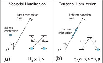
Another interesting situation is the opposite case of a purely tensorial Hamiltonian, in which $\alpha_{V}=0$. In practice, the interaction involves several hyperfine excited states $F^{\prime}$, so that it is possible to choose the detuning such that the various vectorial contributions vanish $\sum_{F^{\prime}}\sigma_{F^{\prime}}\alpha_{V}^{F^{\prime}}\frac{\Gamma}{\Delta_{F^{\prime}}}\simeq 0$, while the total tensorial contribution $\sum_{F^{\prime}}\sigma_{F^{\prime}}\alpha_{T}^{F^{\prime}}\frac{\Gamma}{\Delta_{F^{\prime}}}$ does not. It is then possible to realize a conditional measurement of the alignment in this particular situation. Let us assume that the atoms are prepared in a coherent spin state along $z$. The conjugate transverse components in this case are $\frac{\mathbf{T}^{2}_{2}+\mathbf{T}^{2}_{-2}}{\sqrt{2}}$ and $\frac{\mathbf{T}^{2}_{2}-\mathbf{T}^{2}_{-2}}{i\sqrt{2}}$, since $[\frac{\mathbf{T}^{2}_{2}+\mathbf{T}^{2}_{-2}}{\sqrt{2}},\frac{\mathbf{T}^{2}_{2}-\mathbf{T}^{2}_{-2}}{i\sqrt{2}}]=iN$. We normalize them as previously: $x=(\mathbf{T}_{2}^{2}+\mathbf{T}_{-2}^{2})/\sqrt{N}$ and $p=(\mathbf{T}_{2}^{2}-\mathbf{T}_{-2}^{2})/(i\sqrt{N})$ and assume a circularly polarized probe: $\langle\vec{\mathbf{S}}\rangle=n\vec{z}$.

The result of the integration of Eqs. (12,II) can be found in Ref. Mishina et al. 2007 and is reminded in Appendix B. It yields input-output relationships involving complex spatiotemporal modes for the fields and the atoms. For a thin medium ($\kappa_{T}\ll 1$), they lead to the following input-output relations :

with a tensorial coupling strength given by

($\sum_{F^{\prime}}\alpha_{T}^{F^{\prime}}\frac{\sigma_{F^{\prime}}\Gamma}{8A\Delta_{F^{\prime}}}\sqrt{Nn}$ if several excited states are involved).

The interaction is obviously not QND, since both components of the spin are now modified by the field, and conversely. This arises from the fact that the effective Hamiltonian in this case, $H_{\Lambda}\propto s_{x}x+s_{y}p$, is quite different of the previous vectorial situation $H_{X}\propto s_{z}x$, and now involves both quadratures (Fig. 1). As noted in Dantan and Pinard 2004, this tensorial Hamiltonian corresponds to a linear coupling between two harmonic oscillators which, when resonant, allows for efficient quantum state transfer between atomic and light variables and may be used in quantum memory protocols. As the coupling strength $\kappa_{T}$ is increased, $x^{out}$ and $s_{y}^{out}$ (and $p^{out}$ and $s_{x}^{out}$, respectively) coherently exchange their fluctuations, and it can indeed be shown that, when the collective coupling strength $\kappa_{T}$ is large, the field fluctuations are efficiently mapped onto the atoms and vice-versa Dantan et al. 2005; Mishina et al. 2007.

However, since the atomic variables evolve during a single-pass “tensorial" interaction, it is a priori not well-suited for QND measurements. Nevertheless, it is still possible to perform a conditional measurement of the alignment by using two ensembles $a$ and $b$ (or by making two successive passes in one ensemble) with opposite mean orientations, such that $H_{int}\propto(x_{a}+x_{b})s_{x}+(p_{a}+p_{b})s_{y}$ and $[x_{a}+x_{b},\;p_{a}+p_{b}]=0$. As will be detailed in the next Sections, this restores the QND character of the interaction. The physical interpretation is that both field quadratures are written onto the atoms in each ensemble, but, because of the opposite orientations, their contributions cancel out, leaving the total alignment components unchanged, while the field still carries out information about both atomic alignment components.

We first consider the double-pass geometry depicted on Fig. 2. A quarter-wave plate is inserted between the cell and the mirror, its neutral axis being aligned along $x$. We assume that the same pulse successively propagates back and forth in the atomic ensemble, with no temporal overlap. This is different from the situation of Refs. Takeuchi et al. 2005; Sherson and Mølmer 2006, where the pulse interacts with itself in the atomic medium, so that the non linear coupling allows for unconditional squeezing. We also note that similar ideas have been proposed for quantum memories and squeezing generation in Ref. Muschik et al. 2006 in the case of a purely vectorial hamiltonian. In Muschik et al. 2006, the second pass is used to couple the second quadrature of light to the atoms. Again, the tensorial situation is quite different, since the Hamiltonian directly couples the two quadratures of light to the atoms. However, due to the $s_{x}x+s_{y}p$ form of the Hamiltonian, in order to perform a QND measurement of the alignment, one has to compensate for extra precession terms, which can be successfully done with a double-pass.

The double-pass interaction subsequently leads to

The measurement of $s_{y}^{out^{\prime}}$ (resp. $s_{x}^{out^{\prime}}$) projects $x^{out^{\prime}}$ (resp. $p^{out^{\prime}}$) in a state with reduced variance $V[x^{out^{\prime}}|s_{y}^{out^{\prime}}]=V[p^{out^{\prime}}|s_{x}^{out^{\prime}}]=1-4\kappa_{T}^{2}+o(\kappa_{T}^{2})$. For a moderate value of $\kappa_{T}=0.35$, these variances are $\sim 0.5$, significantly smaller than the standard quantum limit. A rigorous derivation of the conditional variance, including the terms of order $\kappa_{T}^{2}$ in the input-output relations (29-32), can be obtained from the exact results of (-) and leads to exactly the same conditional variance. The measurement of $x$ performed this way is fully QND only for small values of $\kappa_{T}$, and will only result in a limited squeezing in principle. We now turn to a situation allowing for a QND measurement of the alignment for any value $\kappa_{T}$.

Alternatively, a single-pass interaction can be performed with two atomic cells having opposite orientations - as in Julsgaard et al. 2001 - in order to entangle the alignment components of two atomic ensembles. As shown in Fig. 3b the light pulse propagates through two ensembles (a) and (b) prepared with opposite orientation $\langle\mathbf{F}_{z}^{a}\rangle=-\langle\mathbf{F}_{z}^{b}\rangle=N$, so that the input-output relationships now read

If the probe pulse duration is much longer than the time required to propagate through the two cells, the pulse interacts simultaneously with the two ensembles. In this experimentally accessible situation, the previous relations hold to any order in $\kappa_{T}$, and the measurement is perfectly QND. Similarly to the vectorial situation, measuring $s_{y}^{out}$ squeezes the variance of $x_{a}+x_{b}$ to $2/\left(1+2\kappa_{T}^{2}\right)$. Note that one has $\left[x_{a}+x_{b},p_{a}+p_{b}\right]=i\left(F_{z\,a}+F_{z\,b}\right)2/N=0$, since the two ensembles have opposite orientations. It is therefore possible to squeeze not only the fluctuations of $x_{a}+x_{b}$, but also those of $p_{a}+p_{b}$. As can be seen from Eq. (40), sending a second pulse and detecting $s_{x}^{out}$ instead of $s_{y}^{out}$ allows for squeezing $p_{a}+p_{b}$, leaving the alignment of the two ensembles entangled. The expected value of entanglement obtained is $\Delta_{EPR}=\Delta^{2}\left(x_{a}+x_{b}\right)+\Delta^{2}\left(p_{a}+p_{b}\right)=4/\left(1+2\kappa_{T}^{2}\right)<4$. Note that the result is the same as in the vectorial situation of Julsgaard et al. 2001, but the physical situation is rather different, since the tensorial situation requires a double-pass for the alignment measurement to be completely QND.

For a single pass and in the case of a non-zero $\kappa_{V}$, the input-output relations read to first order in $\kappa_{V},\kappa_{T}$

In the double-pass geometry described in Sec. 3, the vectorial contributions cancel out and Eqs. (34-37) are left unchanged, so that the alignment can still be conditionally squeezed in this scheme. In the double-cell configuration, the vectorial contributions to the field evolution (Faraday rotation) naturally cancel out, but the vectorial contributions to the atom evolution (light-shifts) do not. However, a $z$-aligned magnetic field with Larmor frequency $\Omega_{L}=-\frac{\sigma\Gamma}{8A\Delta}\alpha_{V}S_{z}$ can compensate for these light-shifts.

Another experimentally relevant issue is the measurement of the Stokes parameters fluctuations. Technical noise is in general smaller than the quantum fluctuations of light only for higher-frequency components (typically above 0.1-1 MHz). It is therefore important to consider whether the schemes proposed in Sec. IV.2 and Sec. IV.3 can be extended to non-zero frequency noise measurements. In the double-cell configuration, it can easily be done by means of a $z$-aligned magnetic field. The Larmor precession couples $x$ and $p$, but in the frame rotating at $2\Omega$ ($\Omega$ is defined by $\hbar\Omega=\mu B_{z}$, where $\mu$ is the magnetic moment of the ground level and $B_{z}$ the magnetic field value). The input-output relations (38-41) then remain unchanged when making the substitution $x\rightarrow(x)_{2\Omega}=x\;\cos(2\Omega t)+p\;\sin(2\Omega t),$ $p\rightarrow(p)_{2\Omega}=p\;\cos(2\Omega t)-x\;\sin(2\Omega t),$ etc. It is thus possible to measure in a QND manner the atomic operators $x_{2\Omega}$ and $p_{2\Omega}$ through their imprints on the sidebands components of $S_{x}$ or $S_{y}$. Unfortunately, this technique cannot be used in the double-pass configuration, since the magnetic field would have to be reversed between the first and the second pass, which is not very realistic experimentally. However, if measurements of the Stokes operators at non-zero frequency are more easily shot-noise limited, it was shown in Geremia et al. 2004 that strong spin-squeezing could still be obtained experimentally in a zero-magnetic field/frequency situation.

We now discuss the intrinsic limitations brought by spontaneous emission noise in the tensorial Hamiltonian case. For the sake of simplicity we study the case of a $1\rightarrow 0,1$ transitions, with atoms oriented along $z$. Using the Heisenberg-Langevin evolution equations and the quantum regression theorem, we obtain for a $1\rightarrow 0$ transition (for which $\alpha_{V}=-1/2$, $\alpha_{T}=-1$ and $\kappa_{T}=\kappa_{V}\sqrt{2}\equiv\kappa_{0}$):

with $\varepsilon_{a}=-\frac{\kappa_{0}\Gamma}{\Delta}\sqrt{\frac{n}{N}}$, $\varepsilon_{p}=-\frac{\kappa_{0}\Gamma}{\Delta}\sqrt{\frac{N}{n}}$ and $f_{x,p}$, $f_{s_{x},s_{y}}$ standard vacuum noise operators with variance unity.

For the $1\rightarrow 1$ transition, one has $\alpha_{V}=-3/4$ and $\alpha_{T}=3/2$, so that $\kappa_{T}=-\kappa_{V}\sqrt{2}\equiv\kappa_{1}$ and similar equations can be derived. Choosing the detunings such that $\kappa_{0}=\kappa_{1}\equiv\kappa/2$ cancels the vectorial terms finally yields the following input-output relationships

with $\varepsilon_{a}=\frac{\kappa\Gamma}{2}\sqrt{\frac{n}{N}}\left(\frac{1}{\Delta_{1}}-\frac{1}{\Delta_{0}}\right),\hskip 2.84544pt\varepsilon_{p}=\frac{\kappa\Gamma}{2}\sqrt{\frac{N}{n}}\left(\frac{1}{\Delta_{1}}-\frac{1}{\Delta_{0}}\right)$ and $\varepsilon^{\prime}=-\kappa\frac{\Gamma}{4}\left(\frac{1}{\Delta_{1}}+\frac{1}{\Delta_{0}}\right)$. One retrieves beamsplitter-like relations for the losses, similar to those of Duan et al. 2000. $\varepsilon_{p}$ simply describes absorption of the probe caused by spontaneous emission : the probe field is damped by a factor $\sqrt{1-\varepsilon_{p}}$, and some uncorrelated vacuum noise $\sqrt{\varepsilon_{p}}f_{s_{x},s_{y}}$ is consequently added, as for the propagation through a beamsplitter with transmission $\sqrt{1-\varepsilon_{p}}$. $\varepsilon_{a}$ describes the symmetrical process for the atoms : the probe, because of spontaneous emission, induces optical pumping towards a $z$-aligned coherent spin state (which is similar to mixing the probe with some vacuum). A difference with the vectorial situation is the presence of small contamination terms $\varpropto\varepsilon^{\prime}$. They also correspond to optical pumping processes which tend to align $x$ and $p$ along $s_{x}$ and $s_{y}$. To minimize the effect of spontaneous emission noise, one has to choose $n\sim N$ in order to have $\varepsilon_{a}\sim\varepsilon_{p}$, as in Ref. Duan et al. 2000. Finally, the total spontaneous emission contribution in the double-pass or double-cell configurations is finally obtained by doubling $\varepsilon_{a}$, $\varepsilon_{p}$ and $\varepsilon^{\prime}$ in the above equations.

Based on these considerations we discuss the values of squeezing or entanglement that can be expected in experiments with ⁸⁷Rb. We assume an interaction on the $D_{2}$ line with the atoms in the $F=1$ ground state. For room temperature vapor cells, taking into account the Doppler broadening, no detuning allows for completely canceling $\kappa_{V}$. On the contrary, for cold atoms with negligible Doppler broadening, $\kappa_{V}$ can be canceled for a probe laser blue-detuned by $\Delta_{0}=\mathrm{38}$ MHz from the $F^{\prime}=0$ excited level (red-detuned by 34 MHz from $F^{\prime}=1$ and 191 MHz from $F^{\prime}=2$). For typical values for the density and volume ($10^{11}$ cm^-3 and $0.5$ mm³) of a cold atom cloud produced using a magneto-optical trap (the latter being switched off during the measurement), leading to $N=0.5\times 10^{8}$ and taking a pulse of intensity 1 $\mu$W and duration $0.5$ $\mu$s containing $n\sim 0.5\times 10^{8}$ photons (saturation parameter $\sim 10^{-3}$, considering a cross-section $A=1$ mm²), the previous calculations predict $\kappa_{T}\sim-0.42$ and $\sim-5dB$ of squeezing in the quantum fluctuations of $\mathbf{T}^{2}_{2}+\mathbf{T}^{2}_{-2}$ or $\mathbf{T}^{2}_{2}-\mathbf{T}^{2}_{-2}$. Higher values of $\kappa_{T}$ (and hence higher squeezing values) can be reached for longer probe pulses, provided that the duration of the pulses remains smaller than the relaxation time of the Zeeman coherence, or by the use of a dipole trap to increase the optical depth de Echaniz et al. 2005. For these parameters, in a double-pass or double-cell configuration, $\varepsilon_{a}=\varepsilon_{p}=0.14$ and $\varepsilon^{\prime}\lesssim 10^{-4}$ (the contribution of the $F^{\prime}=2$ level is $\sim 30$ times smaller than those of the $F^{\prime}=0,1$ levels, and is not considered). As the fluctuations are predicted here to be reduced by a factor smaller than $\sim 1/0.14$, the noise added by spontaneous emission can be neglected.

For the sake of comparison, we now discuss the relative strengths of tensorial and vectorial conditional measurements. In atomic vapors close to room temperatures, the detuning is usually chosen bigger than the doppler broadening in order to avoid absorption Julsgaard et al. 2001. It implies that the detuning has to be large as compared to the hyperfine structure, and, since one has $\sum_{F^{\prime}}\sigma_{F^{\prime}}\alpha_{T}^{F^{\prime}}=0$ for alkali atoms, it means that $\kappa_{T}\propto\sum_{F^{\prime}}\sigma_{F^{\prime}}\alpha_{T}^{F^{\prime}}/\Delta_{F}^{\prime}\sim 0$, i.e. the effective Hamiltonian is then almost purely vectorial. This situation is obviously much more favorable for orientation than for alignment squeezing.

However, for a doppler-free medium, it is possible to reduce the detuning while maintaining a small absorption. In this case, as can be seen from Fig. 4, both $\kappa_{T}$ and $\kappa_{V}$ (and hence alignment and orientation squeezing) may have similar values. To compare these values, we consider the case of a purely tensorial Hamiltonian (i.e $\kappa_{V}=0$, obtained for $\Delta_{0}=\mathrm{38}$ MHz, $\overline{\Delta_{0}}=13.2$), and the case of a purely vectorial one (i.e $\kappa_{T}=0$, obtained for $\Delta_{0}=\mathrm{222}$ MHz, $\overline{\Delta_{0}}=77$). In the first one, for the experimental parameters given above, $\kappa_{T}=-0.42$, $\kappa_{V}=\mathrm{0}$ and $\varepsilon_{p}=\varepsilon_{a}=0.14$ whereas in the second , $\kappa_{T}=\mathrm{0}$ , $\kappa_{V}=0.03$ and $\varepsilon_{p}=\varepsilon_{a}=0.01$. This shows that the common idea that the vectorial coupling strength is bigger than the tensorial one is not necessarily true for cold atom samples when the hyperfine structure is taken in account.

References

- Dantan et al. (2003) A. Dantan, M. Pinard, V. Josse, N. Nayak, and P. Berman, Phys. Rev. A 67, 045801 (2003).
- Dantan et al. (2006) A. Dantan, J. Cviklinski, E. Giacobino, and M. Pinard, Phys. Rev. Lett. 97, 023605 (2006).
- Kozhekin et al. (2000) A. Kozhekin, K. Mølmer, and E. Polzik, Phys. Rev. A 62, 033809 (2000).
- Dantan and Pinard (2004) A. Dantan and M. Pinard, Phys. Rev. A 69, 043810 (2004).
- Dantan et al. (2005) A. Dantan, A. Bramati, and M. Pinard, Phys. Rev. A 71, 043801 (2005).
- Mishina et al. (2007) O. Mishina, D. Kupriyanov, J. Muller, and E. Polzik, Phys. Rev. A 75, 042326 (2007).
- Kuzmich et al. (2000) A. Kuzmich, L. Mandel, and N. Bigelow, Phys. Rev. Lett. 85, 1504 (2000).
- Duan et al. (2000) L.-M. Duan, J. Cirac, P. Zoller, and E. Polzik, Phys. Rev. Lett. 85, 5643 (2000).
- Thomsen et al. (2002) L. Thomsen, S. Mancini, and H. Wiseman, Phys. Rev. A 65, 061801(R) (2002).
- Geremia et al. (2004) J. Geremia, J. Stokton, and H. Mabuchi, Science 304, 270 (2004).
- Julsgaard et al. (2001) B. Julsgaard, A. Kozhekin, and E. Polzik, Nature (London) 413, 400 (2001).
- Kuzmich et al. (1999) A. Kuzmich, L. Mandel, J. Janis, Y. Young, R. Ejnisman, and N. Bigelow, Phys. Rev. A 60, 2346 (1999).
- Kupriyanov et al. (2005) D. Kupriyanov, O. Mishina, I. Sokolov, B. Julsgaard, and E. Polzik, Phys. Rev. A 71, 032348 (2005).
- de Echaniz et al. (2005) S. de Echaniz, M. Mitchell, M. Kubasik, M. Koschorreck, H. Crepaz, J. Eschner, and E. Polzik, J. Opt. B 7, S548 (2005).
- Duan et al. (2001) L.-M. Duan, M. D. Lukin, J. I. Cirac, and P. Zoller, Nature 414, 413 (2001).
- Chaneliere et al. (2005) T. Chaneliere, D. N. Matsukevich, S. D. Jenkins, S.-Y. Lan, T. A. B. Kennedy, and A. Kuzmich, Nature 438, 833 (2005).
- Ourjoumtsev et al. (2006) A. Ourjoumtsev, R. Tualle-Brouri, J. Laurat, and P. Grangier, Science 312, 83 (2006).
- Neergaard-Nielsen et al. (2006) J. S. Neergaard-Nielsen, B. M. Nielsen, C. Hettich, K. Mølmer, and E. Polzik, Phys. Rev. Lett. 97, 083604 (2006).
- Budker et al. (1998) D. Budker, V. Yashchuk, and M. Zolotorev, Phys. Rev. Lett. 81, 5788 (1998).
- Auzinsh et al. (2004) M. Auzinsh, D. Budker, D. Kimball, S. Rochester, J. Stalnaker, A. Sushkov, and V. Yashchuk, Phys. Rev. Lett. 93, 173002 (2004).
- Budker et al. (2000) D. Budker, D. Kimball, S. Rochester, and V. Yashchuk, Phys. Rev. Lett. 85, 2088 (2000).
- Yashchuk et al. (2003) V. Yashchuk, D. Budker, W. Gawlik, D. Kimball, Y. Malakyan, and S. Rochester, Phys. Rev. Lett. 90, 253001 (2003).
- Happer (1972) W. Happer, Rev. Mod. Phys. 44, 169 (1972).
- Omont (1997) A. Omont, Progress in Quantum Electronics 5, 69 (1997).
- Cohen-Tannoudji and Barrat (1961a) C. Cohen-Tannoudji and J. Barrat, Journal de Physique 22, 329 (1961a).
- Cohen-Tannoudji and Barrat (1961b) C. Cohen-Tannoudji and J. Barrat, Journal de Physique 22, 443 (1961b).
- Laloe and Cohen-Tannoudji (1967a) F. Laloe and C. Cohen-Tannoudji, Journal de Physique 28, 505 (1967a).
- Laloe and Cohen-Tannoudji (1967b) F. Laloe and C. Cohen-Tannoudji, Journal de Physique 28, 722 (1967b).
- Grangier et al. (1998) P. Grangier, J. Levenson, and J.-P. Poizat, Nature (London) 396, 537 (1998).
- Poizat et al. (1994) J.-P. Poizat, J.-F. Roch, and P. Grangier, Ann. Phys. (Paris) 19, 265 (1994).
- Julsgaard (2003) B. Julsgaard, Entanglement and quantum interactions with macroscopic gaz samples, PhD thesis, University of Copenhagen (2003).
- Takeuchi et al. (2005) M. Takeuchi, S. Ichihara, T. Takano, M. Kumakura, T. Yabuzaki, and Y. Takahashi, Phys. Rev. Lett. 94, 023003 (2005).
- Sherson and Mølmer (2006) J. Sherson and K. Mølmer, Phys. Rev. Lett. 97, 143602 (2006).
- Muschik et al. (2006) C. Muschik, K. Hammerer, E. Polzik, and J. Cirac, Phys. Rev. A 73, 062329 (2006).