KYUSHU-HET-107
KUNS-2074
Holographic Construction of Technicolor Theory
Takayuki Hirayama1** * e-mail: hirayama@th.physik.uni-bonn.de and Koichi Yoshioka2†† † e-mail: yoshioka@gauge.scphys.kyoto-u.ac.jp
1
Physikalisches Institut der Universitaet Bonn,
Nussallee 12, 53115 Bonn, Germany
2
Department of Physics, Kyushu University, Fukuoka
812-8581, Japan
2
Department of Physics, Kyoto University, Kyoto 606-8502, Japan
We construct a dual description of technicolor theory based on the D4/D8 brane configuration. A strongly-coupled technicolor theory is identified as the effective theory on D-branes, and from the gauge/gravity correspondence, we explore the weakly-coupled holographic description of dynamical electroweak symmetry breaking. It is found from the D-brane probe action that the masses of and bosons are given by the decay constant of technipion, and the technimesons become hierarchically heavy. Moreover, the couplings of heavier modes to standard model fermions are rather suppressed. The oblique correction parameters are also evaluated and found to be small except for the parameter, which can be reduced by modifying the model. The fermion fields are introduced at the intersections of D-branes and their masses are generated via massive gauge bosons from open strings stretching between D-branes.
1 Introduction
Future particle experiments such as the Large Hadron Collider (LHC) will provide important data on the sector of electroweak gauge symmetry breaking. In the Standard Model (SM), the elementary scalar fields, the Higgs bosons, are responsible for the symmetry breaking, though there is a well-known problem of gauge hierarchy between the Planck and electroweak scales. One of the alternatives to elementary Higgs is the dynamical electroweak symmetry breaking induced by a strongly interacting gauge theory, the technicolor scenario [1]. It has been known, however, that technicolor models often suffer from the difficulty of passing the electroweak precision tests through the oblique corrections [2]. Since a strongly interacting dynamics is involved in the analysis, it is still an important issue whether a realistic technicolor model can be constructed.
The recent development of brane physics in string theory provides us an alternative way to analyze strong coupling region of gauge theory via weakly-coupled gravitational description. The original proposal of the gauge/gravity correspondence claims that the supergravity on AdS is dual to the four-dimensional super Yang-Mills theory with large and large ’t Hooft coupling [3, 4], and various derivatives have been discussed in the literature. In particular, there have been attempts to construct a holographic description of Quantum Chromo Dynamics (QCD), which is a strongly interacting gauge theory at low energy regime. Among them the model of Ref. [5] realizes the non-abelian chiral symmetry breaking from the D-brane geometry and predicts the vector meson mass spectrum and interactions which are comparable with the experimental data.
The dynamical electroweak symmetry breaking in the technicolor scenario is regarded as a scale-up version of chiral symmetry breaking in QCD. In this paper, we construct a dual description of technicolor by applying the holographic gauge/gravity correspondence. Since the holographic description is in the weakly coupling regime, it enables us to treat the non-perturbative dynamics of technicolor theory in a perturbative way. Furthermore, a dual technicolor theory is constructed from the D-brane configuration and the gauge/gravity correspondence makes it possible to analyze the technicolor dynamics in quantitative treatment. In order to gauge the flavor chiral symmetry in QCD, it is assumed that the six-dimensional extra space in string theory are compactified. In the original gauge/gravity correspondence, this procedure is expected to introducing a cutoff near the AdS boundary and giving appropriate boundary conditions at the cutoff. From the holographic description, we can calculate the strength of gauge couplings and the mass spectra of SM gauge bosons and composites fields which are analogous to QCD-like mesons in the technicolor theory. The gauge bosons other than the SM ones are shown to become hierarchically heavy. We also discuss how to introduce SM quarks and leptons into our scheme and compute their minimal couplings to the SM gauge bosons and heavier modes. The fermion masses are induced by a similar mechanism to the extended technicolor theory [6]. The oblique correction parameters are explicitly calculated and are found to be small except for the parameter. We comment on possibilities to suppress the parameter in our model.
This paper is organized as follows. In the next section we describe the D-brane configuration to define our technicolor theory as the effective theory on the D-branes. In Section 3, its holographic dual description is explored where the probe branes describe the action below the scale of techniquark condensation. Solving the equations of motion both approximately and numerically, we show how the SM gauge bosons and composite fields are described and evaluate their masses and interactions. Section 4 discusses an idea of introducing SM matter fields by utilizing additional D-branes. We derive the Lagrangian for SM matter fields from the holographic description and estimate their masses and gauge interaction strength. In Section 5 we examine whether the model passes the electroweak precision tests by evaluating oblique corrections to the electroweak observables. Some comparison with the so-called higgsless models [7] is mentioned in Section 6. Finally we conclude and discuss open issues in the last section.
2 D-brane Configuration: The Gauge Sector
In this section we describe the D-brane configuration in the flat space background of type IIA string theory which realizes a technicolor scenario as the effective theory on the D-branes. The configuration consists of D4, D8 and anti-D8 () branes. The coincident D4-branes realizes pure Yang-Mills theory‡‡ ‡ The overall factor decouples. in compactifying one spacial direction on a circle with the anti-periodic boundary condition of the fermionic variable on the D4-branes. The boundary condition leads to the fermion zero mode being projected out, and the scalar modes become massive due to supersymmetry-breaking quantum effects. We thus identify this as the technicolor gauge symmetry. In this work we refer to D4-branes as the technicolor branes. The techniquarks are provided by introducing sets of D8 and -branes. They are localized at different (possibly opposite) points in the direction and the open string stretching between the technicolor D4 and D8 () branes provides a four-dimensional massless chiral (anti-chiral) fermion, i.e. a pair of techniquarks, as the lowest massless mode. The cartoon of D-brane configuration is shown in Fig. 1.

The five-dimensional transversal directions to the technicolor D4-branes are assumed to be compactified in order to have a finite Newton constant in four dimensions. Then the gauge fields on the D8-branes are dynamical in four dimensions and induce gauge symmetry. Similarly we have gauge symmetry on the -branes. The left (right) handed techniquark from D4-D8 (D4-) branes is bi-fundamentally charged under [].
where the blanks denote singlet representations hereafter. The symmetry is expected to be dynamically broken by the condensation of techniquarks and thus the electroweak gauge symmetry is embed in . In addition to the gauge fields, there are scalar and spinor modes on the D8 and -branes. These fields are assumed to receive loop-induced masses since supersymmetry is broken and their mass terms are not prohibited by any symmetry. In the limit, there are no tachyonic states, but for a finite there is an instability caused by the closed-string exchange between D8 and -branes. The mode associated with this instability could are stabilized by some mechanism in string theory such as fluxes, Casimir effects or non-perturbative effects. Later, additional D4-branes which provide quarks and leptons are introduced (D4’ in Fig. 1) and the positions of D4’-branes are the moduli which should also be stabilized. It is assumed that Ramond-Ramond charges and the cosmological constant are both canceled by properly introducing D-branes, anti D-branes or orientifolds away from the technicolor branes.
Depending on how to embed the electroweak gauge symmetry in , different types of phenomenological models can be constructed. In this paper we investigate the simplest choice where the number of D8-branes is minimal, i.e. . In this case there are two ways to realize the electroweak symmetry. The first choice is identifying as the electroweak symmetry in the SM and as the hypercharge . The other is the identification that is the electroweak symmetry and is an extra which is used to realize the desired symmetry breaking pattern. While both choices of embedding are worth consideration, in this paper we investigate the first pattern of electroweak symmetry breaking.
The overall ’s in are related to the positions of D8 and -branes and supposed to be broken. To have the electroweak symmetry, is broken down to with an adjoint Higgs field at a high scale. Notice that there is an adjoint scalar field on the -branes which can play as the Higgs field inducing such breaking. Thus the viable gauge symmetry becomes under which the techniquarks have the following quantum charges:
Below the technicolor scale , at which the gauge coupling of technicolor gauge theory becomes strong, the techniquarks are expected to be condensed, i.e. (), and the dynamical electroweak symmetry breaking is realized
| (2.1) |
3 Holographic Dual Description of Technicolor
The holographic dual description of the technicolor theory given above is obtained from the gauge/gravity correspondence, that is, by replacing the technicolor D4-branes with their near horizon geometry. The near horizon geometry of D4-branes compactified on with supersymmetry-breaking boundary condition [8] is
| (3.1) | |||
and the dilaton and the Ramond-Ramond four-form field strength are given by
| (3.2) |
The D4-branes extend to the four-dimensional spacetime () and the direction which is compactified on a circle with the radius :
| (3.3) |
The coordinate is a radial direction transversal to the D4-branes, and , and are the metric, volume and line element of the unit four-dimensional sphere. The constant parameter is proportional to the number of D4-branes . The technicolor gauge coupling at the compactification scale is determined by the string coupling and the string length and is given by . The holographic dual description is valid in the region [9].
The existence of technicolor D4-branes modifies the geometry near themselves, that is, a throat is developed. Therefore we are looking at the geometry of throat. This geometry is trustful in the region () and the contribution to the four-dimensional Planck constant is negligible compared with the bulk contribution as long as the throat volume is much smaller than the bulk one without the throat. If one supposes that the size of compactification is the same order of the string length except for the direction, the volume of six-dimensional extra space is . Then as long as the maximal value of is smaller than (), the throat has a suppressed size, as desired.
Since a large value of () is taken for the validity of holographic description, the D8 and branes are treated as probes in the D4 geometry. In the flat space the D8-branes are localized at a constant and still reside in the same point on the curved geometry since the metric coefficients do not explicitly depend on . Then the coefficient of goes to zero at , and the D8-branes are smoothly connected with the -branes at this point and make up smooth D8-branes, see Fig. 2.

In the holographic dual description of technicolor theory with a large ’t Hooft coupling, the connection of D8 and -branes is interpreted as the dynamical breaking of symmetry to the diagonal one . This is because only the simultaneous rotation of D8 and -branes remains intact. In Ref. [5], the smoothly connected D8-brane describes the chiral symmetry breaking in QCD and provides the meson spectrum and interactions. In the present model (), the D8-branes action describes the dynamical electroweak symmetry breaking in technicolor theory, and provides the SM gauge bosons (the photon, and bosons) as well as technimesons below the scale of the techniquark condensation.
The probe D8-brane action is given by the Dirac-Born-Infeld action in the curved geometry. We focus on the gauge sector while scalars and spinors on the branes may become massive due to high-scale supersymmetry breaking. The relevant action up to the quadratic level is obtained from the Yang-Mills approximation of the Dirac-Born-Infeld action
| (3.4) |
where is the tension of D8-brane, () is the induced metric and is the field strength of gauge fields on the probe D8-branes. It is noted that there exists a single gauge theory on the connected D8-branes. The D8-branes are localized at and the induced metric is given by
| (3.5) | |||
| (3.6) |
where we have defined a new dimensionless coordinate which goes along the D8-brane ()§§ § and in the new coordinates system.. One may understand that the D8 () branes are described in the () region and they are smoothly connected with each other at . The four-dimensional gauge action below the compactification scale is obtained by integrating over extra five dimensions (the and directions). The metric has the invariance of and Kaluza-Klein modes in the compactification are parameterized by angular momenta along . The nonzero momentum modes are heavy and in the following discussion only the zero momentum modes may be relevant. We therefore focus on -invariant modes and evaluate the integration to obtain the five-dimensional effective action
| (3.7) | |||
| (3.8) |
where the Lorentz indices , are contracted by the four-dimensional Minkowski metric hereafter. Here we have dropped gauge fields along the directions which are expected to obtain masses from supersymmetry breaking and compactification. The gauge boson has been rescaled such that the coefficient of kinetic term is properly except for the factor. As mentioned in the introduction, the boundaries of extra dimension have been introduced at and , and the bulk geometry outside the throat is integrated out. The parameters and reflect the volume of D8 and -branes in the extra dimension, and the four-dimensional gauge couplings of are inversely proportional to , as seen below. We have also introduced a parameter in the definition of gauge coupling which represents how the D8-branes extend in the bulk.
In order to have the four-dimensional effective action integrating over the direction, one needs to specify the boundary conditions of gauge fields at and . Since the () region is understood as the D8 () branes on which the () gauge symmetry is realized, it is found that the following conditions are appropriate for the present situation (/ denotes the Neumann/Dirichlet boundary condition):
| (3.9) | ||||||
where and are the and gauge fields, respectively. We take the gauge hereafter. In this gauge, the scalar zero modes in are taken into account. While has such a scalar mode which is interpreted as the Nambu-Goldstone boson associated with the global axial symmetry, there is nonzero mixed gauge anomaly of and the scalar zero mode becomes massive due to the Green-Schwarz mechanism. A Dirichlet boundary condition may be interpreted as taking a scalar expectation value which causes symmetry breaking infinite.
Expanding the gauge fields with orthonormal wavefunctions as , we obtain the equations of motion for the eigenmodes from the above action
| (3.10) |
with the normalization condition
| (3.11) |
The mass of the eigenmode is given by . The zero-mode wavefunctions are easily found and are proportional to
| (3.12) |
The existence of two massless modes inherits the fact that there are originally two gauge sectors . The wavefunctions and are localized in the positive and negative region respectively and then correspond to the wavefunctions of and gauge fields in the technicolor side. Furthermore, () becomes normalizable as long as () is finite. This is consistent with the facts that () reflects the volume of D8 () branes and the gauge fields on the D8 () branes become dynamical in four dimensions if the volume of D8 () is finite along the extra dimensions.
Solving the equations of motion (3.10), we find that the Kaluza-Klein decompositions of gauge fields take the following forms:
| (3.13) | ||||
| (3.14) | ||||
| (3.15) |
For the boundaries far away from the origin (), the lower mode wavefunctions are approximately given by
| (3.16) | ||||
| (3.17) | ||||
| (3.18) |
and the mass eigenvalues are
| (3.19) |
where , roughly independent of . It is interesting to notice that the masses of other Kaluza-Klein excited gauge bosons become and hierarchically larger than the SM gauge boson eigenvalues (3.19). These formulas are found to well fit the numerical results within a few percent errors in calculating the gauge coupling constants in later sections.
We have found that there are four light gauge bosons , and in addition to an infinite number of heavy Kaluza-Klein modes (). For a schematic pattern of mass spectrum, see Fig. 4.


The wavefunction of the massless mode is constant ( independent), which is exactly given by , and is understood as the unbroken gauge boson, the photon. With the formulas of wavefunctions, we can rewrite the third-component gauge boson as
| (3.20) |
where we have introduced
| (3.21) |
As explained before, the wavefunctions and respectively correspond to and in which the electroweak gauge symmetry is contained as and . Therefore the expression (3.20) indicates that is interpreted as the boson in the SM with the identification that is the Weinberg angle. It is noted here that the photon and the boson are unified into a single gauge field on the connected D8 branes in the present model. Interestingly enough, the identification of the Weinberg angle (3.21) is consistent with the prediction of mass spectrum (3.19), i.e. the relation is indeed satisfied. This fact confirms that correspond to the bosons in the SM.
Substituting the Kaluza-Klein decomposition in the five-dimensional action, we obtain the four-dimensional effective theory of the gauge sector
| (3.22) |
where () and . We have not written down the four-point gauge interaction operators explicitly. The strengths of self gauge interactions among the electroweak gauge bosons are determined by the wavefunction profiles
| (3.23) | ||||
| (3.24) | ||||
| (3.25) | ||||
| (3.26) |
Since the wavefunctions are almost constant except for the small region and quickly goes to zero for negative , the following approximations hold: and . Thus the electroweak gauge couplings for () and () are found
| (3.27) |
Therefore it is again consistently understood that and represent the volumes of D8 and branes, respectively. We will demonstrate in later section the numerical results of mass spectrum and how etc. are close to the weak gauge coupling which is determined from the fermion vertices.
Let us turn to discuss the heavier gauge bosons. The lightest modes among () comes from the 2nd excited modes in and are referred to as the bosons. A slightly heavier mode comes from the 2nd excited mode in ; we call it the boson. The numerical analysis shows that the masses of higher Kaluza-Klein modes including the and bosons are around the compactification scale and hierarchically larger than the SM gauge boson masses (Fig. 4). For example, we have for . The overall gauge field is irrelevant to the electroweak gauge symmetry and we will not consider Kaluza-Klein modes from in the following discussion. The wavefunctions of heavy gauge bosons are found to be localized at which indicates, from the gauge/gravity correspondence, that these fields are interpreted as composites (technimesons) in the technicolor theory. The couplings of bosons to the SM sector are generally suppressed since their wavefunctions are localized around and have small overlap with those of the electroweak gauge bosons. For example the triple gauge boson coupling between and is evaluated as
| (3.28) |
for (in fact, somehow independently of ). In this way, the above discussion shows that in the dual description the dynamical electroweak symmetry breaking through the techniquark condensation is holographically realized. The observed value of the Weinberg angle can be obtained by taking and the weak gauge coupling by choosing .
The decay constant , which is an analogue of the pion decay constant of QCD in the technicolor theory, can be calculated in a similar way to Ref. [5]. The Nambu-Goldstone bosons, which are eaten by the and bosons, are originated from and have the wavefunction proportional to []. Since this wavefunction is localized at , the value of decay constant does not depend on and is same as that in Ref. [5]:
| (3.29) |
where the last equation is obtained from (3.8). Using this decay constant we can express the mass spectrum as
| (3.30) |
with . The last equation suggests the dynamical scale of technicolor theory is around . On the other hand, the masses of , bosons and composites fields (denoted by ) are estimated from the technicolor theory that
| (3.31) | |||
| (3.32) |
From the consistency of these two expressions of spectrum, we find that the holographic gravity dual provides a calculable and compatible framework to technicolor theory.
The decay constant is given in terms of and . It is noticed that the holographic description is valid when the ’t Hooft coupling is large, which might give a constraint on through eq. (3.29). For example, a large ’t Hooft coupling leads to . When and as an example, one obtains . If another condition () is taken into account, we would have a slightly severe constraint on the decay constant.
Finally, several comments are in order. One may wonder about the unitarity. The general argument in [7] can be applied to our model as well and then the unitarity of massive gauge theory is formally recovered by Kaluza-Klein gauge bosons . To avoid the breakdown of perturbative unitarity, the compactification scale would be set below a few TeV and . In addition to technimesons, there are also technibaryons. Refs. [10] study baryons from holographic descriptions of QCD and the first reference in Refs. [10] shows that baryons are heavier than the meson after taking into account the Chern-Simons term, as expected. If we apply their analyses to our case, we would find technibaryons are heavier than the boson.
4 The Matter Sector
4.1 D-brane configuration
To complete the realization of the SM (without the Higgs), we next consider the introduction of SM matter fields. Let us add some number of D4-branes into the previous brane configuration for the gauge sector (see Fig. 1) in the flat space. The added branes are parallel to but separated from the technicolor D4-branes. In this work these additional D4-branes are referred to as the flavor branes. Then at the intersection of a flavor D4-brane with D8 or , we have a massless chiral or anti-chiral fermion which transforms as the fundamental representation under or . With appropriate numbers of flavor branes being introduced, such chiral fermions are identified with the SM matter fields. There are also open strings which connect the flavor and technicolor branes. The fermion mass terms are generated by massive gauge fields from these open strings, which is a similar mechanism in the extended technicolor theory.
We introduce one flavor D4-brane at one point (for a lepton) and three coincident D4-branes at another place (for a quark). These D4-branes and the technicolor D4-branes are separated to each other in the extra dimensions, particularly in the direction. At the four intersection points among D4’lepton, D4’quark, D8 and , we have four types of chiral fermions, , , and :
where and are the gauge symmetries on the D4’lepton and D4’quark branes, respectively. Similar to the technicolor branes, the effective theories on the flavor D4-branes are pure Yang-Mills theories, since scalar and spinor fields on the flavor branes become massive due to the anti-periodic boundary conditions for spinors imposed along the direction (). Naively the leptons and quarks do not have the correct hypercharges, but we can mix with and also with the overall in , which are identified to the lepton and baryon number gauge symmetries. The quark fields are assigned to have the charge . The mixing depends on how the symmetries are broken down. In this work we assume, for simplicity, that there are two scalar fields at the intersections of flavor branes and the -branes, whose quantum numbers are respectively given by under and under , and their vacuum expectation values are taken infinity. In this case the gauge fields of and of at the intersections become
| (4.1) |
where is the gauge fields of on the branes, and the normalization of and are taken such that the gauge couplings appear in front of the kinetic terms. We then find that the leptons and quarks have the correct hypercharges with taking a simple choice . For example the right-handed quarks have the minimal interaction with the following combination of gauge fields
| (4.2) |
To summarize, the leptons and quarks have charges under the unbroken gauge symmetry as
This is just the SM matter content in one generation. To realize the complete set of three generations, one may further introduce two more sets of flavor D4-branes and repeat the same mixing. It is assumed that ’s are broken down to the diagonal which is identified to the color gauge symmetry in the SM. The original gauge coupling is shifted by the mixing and is finally matched to the experimentally observed value.
4.2 Holographic dual description
We have explained how the SM matter fields are introduced in the technicolor theory from a viewpoint of brane configuration. Its holographic description completes a dual picture of electroweak theory with symmetry breaking caused by strongly-coupled gauge dynamics.
A flavor D4-brane in the near horizon geometry is located at a constant distance away from the origin and extends along the direction as well as the non-compact four-dimensional space. The -th flavor D4-brane intersects with the probe D8-brane at two points (). A left (right) handed chiral fermion is located at (). Their quantum charges have been fixed in Section 4.1.
We have presented the scheme in the technicolor side that on the brane is mixed with ’s on flavor branes to have the right hypercharge assignment. The holographic description of the mixing (4.1) is simply given by replacing and with and , i.e.
| (4.3) |
where is the gauge field on flavor D4-branes. We have taken the normalization for such that the gauge coupling appears in front of the kinetic term. Since the direction is compactified on and gauge fields have periodic boundary conditions, have a constant profile along the flavor D4-branes. The photon and boson (and the excited modes ) are united in and thus propagate on the flavor D4-branes. These corrections have the same implication in the technicolor side where the gauge coupling of is shifted. From (3.20), we obtain
| (4.4) |
where the ellipses denote the terms with bosons. As long as is large enough, is almost equal to one (), which implies from (4.4) that is essentially the gauge boson. In this case the flavor D4-brane action induces an additional kinetic term just for gauge boson and changes the gauge coupling in canonically normalizing the gauge field. The parameter is properly adjusted so that the final gauge coupling constant matches with the observed value [see eq. (3.27)]¶¶ ¶ This contribution is not included in the following analysis. A rough estimation shows that the order of magnitude of is shifted by about one if the gauge coupling on flavor D4-branes is of the same order of . The contribution to oblique correction parameters will be discussed in the next section..
Now we are ready to write down the four-dimensional action for the SM matter fields in the holographic description. We only discuss the left-handed leptons which emerge from the intersection between the connected D8-branes and flavor D4-branes. It is a straightforward extension to include all the matter fields in a completely parallel way. The action of left-handed leptons becomes
| (4.5) |
where , and for left-handed fermions. The parameter ( and ) is used for denoting the effective angle to distinguish it from our parametrization introduced in (3.21). The definition is exactly same as (3.23) from the gauge boson self coupling. The other fermion current couplings are defined from the gauge boson wavefunctions
| (4.6) | ||||
| (4.7) | ||||
| (4.8) |
The weak gauge couplings seem to depend on the position of flavor D4-branes. However the gauge boson wavefunctions are nearly constant in the large region and the flavor universality of electroweak gauge coupling is satisfied with good accuracy unless the flavor branes reside close to the origin . The constant profiles of gauge boson wavefunctions also imply that the electroweak couplings are approximately given by , , and , which is consistent with the SM expressions. We thus find that all the SM matter fields couple to the photon, and bosons with the (almost) correct strength. On the other hand, the couplings to higher Kaluza-Klein gauge bosons are suppressed because their wavefunctions are localized at unlike the SM gauge fields. We will show the numerical results for these behaviors in Section 5.
4.3 Fermion masses
Finally we have a brief comment on a possibility how the masses of matter fermions are generated in the present model. In the extended technicolor theory, the massive gauge bosons associated with the breaking of extended technicolor gauge symmetry mediate the condensation of techniquarks to the SM fermions, leading to their masses where and are the gauge coupling constant and the mass of gauge bosons in the extended technicolor theory.
In our D-brane configuration, we have such massive gauge bosons which originate from open strings stretching between the technicolor D4 and flavor branes. That is seen from the fact that the gauge symmetry is enhanced when the flavor branes attach with the technicolor branes. The gauge boson mass , which is given by the length of an open string, and the induced fermion mass are evaluated as
| (4.9) | |||
| (4.10) |
where is the induced metric on the open string which is localized at a constant . For example, if TeV and are assumed, the flavor branes are located at for the top, charm, and up quarks, respectively. The positions of flavor branes are within the cutoff in the direction. For a small value of , the flavor gauge boson deviates from and the oblique correction parameters may be induced. If one may try to cure this problem, an idea is to realize that the top flavor D4-brane is not parallel to and has some angle against the technicolor D4-brane. In this case, a left-handed fermion can be localized closer to the technicolor brane compared with a right-handed fermion, and one may obtain a heavy fermion mass without leading to large oblique correction parameters. However too close to the origin , the wavefunctions for and bosons are deviated from the constant profiles, and a closer top brane implies that the model would receive a constraint from the measurement of coupling [12]. In addition if one considers the generation mixing, the rare observation of flavor-changing neutral current would provide severer constraints.
5 Electroweak Precision Tests
We have constructed a model of electroweak symmetry breaking, holographically dual to a technicolor theory. It is well known that a technicolor theory usually suffers from the difficulty of passing the electroweak precision tests. Any departure from the SM predictions is severely constrained from the existing experimental data. In particular, for the electroweak gauge symmetry breaking, that is known to be summarized as the oblique correction parameters; , , [2] which are defined by the two-point correlation functions of electroweak gauge bosons, and the vertex correction parameters [11]. In this section, we discuss the tree-level (pseudo) oblique corrections in our holographic technicolor model.
There are four fundamental parameters in the technicolor theory; the electroweak gauge couplings and , the technicolor scale , and the decay constant , which correspond to , , , in the holographic dual description. The fine structure constant and the boson mass are well measured quantities and their values at pole are used to fix and . Therefore we compare our action with the SM action (minus Higgs fields) at pole and parametrize the deviations in the couplings as oblique parameters. We obtain four predictions , , , and as the functions of , and . In the technicolor theory, the predictions are the functions of and one combination of gauge couplings [see eqs. (3.29) and (3.30)]. The charged and neutral current interactions and the boson mass contain four oblique correction parameters , , , and defined in [11]. Since in the holographic description the gauge fields have been set to orthonormal, the oblique parameters are expressed in terms of gauge vertices of SM fermions. From the matter action (4.5), we find the following forms of oblique corrections:
| (5.1) | |||||
| (5.2) | |||||
| (5.3) | |||||
| (5.4) |
with the deviations from the SM form
| (5.5) |
and and at the pole [12]. The effective angle has been replaced with which is defined from the Fermi constant. The observed values of these two angles are almost equal and the difference does not affect the following analysis. Substituting the approximate solutions obtained in Section 3, one has if is satisfied.
Let us first study the case that all the SM matter fields are localized at the same point (and can be separated along direction) and discuss the effects of changing the position of flavor branes later. The numerical results are summarized in Table 1 and Fig. 5.
Table 1 shows the , , parameters with which is fixed by choosing an appropriate value of .


In Fig. 5 the oblique parameters are displayed as the functions of . We have set from the hierarchy between the electroweak and Kaluza-Klein excited gauge bosons. From these results, we find that the oblique parameters except for are roughly constant and small compared with the SM fit: , and [12] (while one could subtract the contribution of Higgs fields). The smallness of parameter is ensured because of the custodial symmetry. The parameter is generally large and positive, but decreases as to the experimentally allowed region for . For , with assuming , and so the validity of holography may not be clear. Table 1 also shows that the self couplings of gauge bosons are consistent with the observed data. Such a result has been mentioned in the previous section with the approximate solutions. The holographic dual description thus recovers the qualitative behavior of technicolor theory against the electroweak precision test. However the holographic theory has some advantages that the oblique correction parameters are easily handled by deforming the model and/or taking other sources to the corrections into account.
In the evaluation of oblique correction parameters, there are other sources, than shown above, which lead to the modification of oblique parameters, in particular, the reduction of parameter. The first is the position of SM fermions in the extra dimensions, i.e. the intersecting point of D8 and flavor D4 branes. The position of flavor branes little affects the tree-level oblique parameters in a large region because the wavefunctions of electroweak massive gauge bosons have almost flat profiles along the extra dimension. If one places the flavor branes at some point closer to the technicolor branes, the parameter is reduced and can be negative, since the fermion couplings to the boson is a bit suppressed. For example, , , and for and . The second possible source is the contribution from the flavor branes. If the gauge field on the flavor D4-brane is just proportional to , an additional kinetic term is absorbed by changing the gauge coupling , i.e. by adjusting . The non-vanishing oblique corrections are induced when the gauge group on the flavor branes differs from , that is, if is different from . From the numerical analysis, we find () for () and . That induces an extra kinetic term for the boson and the parameter is pushed toward negative with an amount of whose size depends on the gauge coupling constant on the flavor D4-branes.
We have also not included the corrections from technimesons. Table 2 shows the numerical evaluation for the masses and coupling constants of Kaluza-Klein excited gauge bosons.
The higher-mode gauge couplings are expressed by the ratios to the corresponding SM couplings. It is found from the table that the tree-level correction to the Fermi constant is roughly and the parameter is shifted toward negative with amount of . Moreover the higher Kaluza-Klein mode couplings to fermions are more suppressed. In a recent paper [13], a possibility is pointed out that may be modified depending on the distance between D8 and -branes. Among various contributions, which effect is dominant depends on the model parameters and the details of calculation is left for future study. A small (and even negative) parameter is expected to be viable if taken into account these modifications of the model.
6 Comparison to Higgsless Models
In this section, we comment on some connections to the so-called higgsless models which are defined in five dimensions [7]. The viable types of higgsless models utilize the AdS5 warped geometry and the electroweak symmetry breaking is caused by appropriate boundary conditions at the infrared (IR) brane.
An analogy to higgsless models in the warped geometry becomes that we have two throats which merge at the IR brane. The two boundaries in our model correspond to two different ultraviolet (UV) branes (the UV and UV’ branes in Fig. 6).
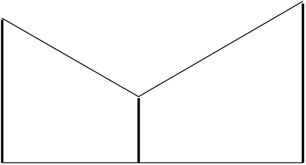
In fact the boundary conditions in our model determine the gauge symmetry above the technicolor scale. In the language of higgsless models, this corresponds to that there exist two different gauge symmetries in the two throat regions, and the boundary conditions at the two UV branes determine what of symmetries are gauged at UV scales.
In the higgsless models, the electroweak gauge symmetry is broken by the boundary conditions imposed at the IR brane. It may be suggested from the gauge/gravity correspondence in string theory that a higgsless model in the AdS5 geometry with boundaries has a dual description in terms of strongly coupled gauge theory. However it is generally difficult to determine the dynamics of technicolor theory. On the contrary to that, in our model, we can identify the technicolor theory and the condensation of techniquarks. That implies in the higgsless models that a specific boundary condition at the IR brane is chosen to connect the gauge fields in the bulks I and II.
The limit of taking , i.e. taking the UV’ brane in Fig. 6 close to the IR brane, might be thought as the reduction to a higgsless model. This is however unlikely since the limit corresponds to a strong coupling limit of the gauge symmetry on the branes.
In the higgsless scenarios, the oblique correction parameters have been explored in the literature. In particular it was pointed out that the parameter is made small if bulk SM matter fields are introduced in a specific way [14]. The situation is similar to our model in which the parameter becomes smaller if we place the flavor D4-branes closer to the technicolor D4-branes. There have been various proposals in the higgsless models to reduce oblique corrections and to avoid a large deviation in the coupling while realizing the heavy top quark. These proposals may offer the suggestions for modifying our model.
7 Conclusions and Discussions
In this paper we have explored a holographic dual description of technicolor theory from the D-brane configuration. The electroweak gauge symmetry is dynamically broken in the D4 background geometry. The holographic description makes it possible to analyze the non-perturbative dynamics of technicolor theory in a perturbative and quantitative way. We have calculated the spectrum of SM gauge bosons and technimesons which are expressed by the technicolor scale and the decay constant. The heavier mode gauge bosons obtain hierarchically larger masses than the SM ones and have suppressed couplings to the SM matter fields. The quarks and leptons have been introduced with the correct hypercharges from the flavor D4-branes and their masses are generated by massive gauge bosons in a similar way to the extended technicolor theory.
The oblique parameters have been numerically computed and found to be small, except for the parameter which significantly deviates from zero and takes a positive value. We have discussed several sources to reduce the parameter (even toward a negative value): the positions of flavor branes, and the contribution to hypercharge kinetic terms from the flavor branes. Another interesting possibility would be to realize bulk SM fermions. For example, with an additional D8-brane introduced, an open string between this new D8 and the electroweak D8 branes induces a pair of vector-like quarks. The bulk fermion mass parameters are tuned by the distance between two D8-branes. The introduction of bulk fermions would also be useful for reducing oblique corrections, realizing the correct couplings of the third generation fermions, suppressing flavor-changing rare processes, and so on.
It is an independent question if a phenomenologically viable model can be constructed by D-brane configurations. The fluxes which stabilize moduli often generate throats and a more realistic model may appear in other throat geometries. As well as other ways of embedding the electroweak symmetry and introducing the SM matter, the applications to higher-scale theory such as grand unified theory would be worthwhile.
Acknowledgements
The authors would like to thank Kang-Sin Choi for collaboration during the early stages of this work. T.H. would like to thank Koji Hashimoto and Akitsugu Miwa for useful discussions. This work is supported by the European Union 6th framework program MRTN-CT-2004-503069 “Quest for unification”, MRTN-CT-2004-005104 “ForcesUniverse”, MRTN-CT-2006-035863 “UniverseNet”, SFB-Transregio 33 “The Dark Universe” by Deutsche Forschungsgemeinschaft (DFG), the grant-in-aid for scientific research on the priority area (#441) “Progress in elementary particle physics of the 21st century through discoveries of Higgs boson and supersymmetry” (No. 16081209) and by scientific grant from Monbusho (No. 17740150).
References
- [1] S. Weinberg, Phys. Rev. D13 (1976) 974; Phys. Rev. D19 (1979) 1277. L. Susskind, Phys. Rev. D20 (1979) 2619. C.T. Hill and E.H. Simmons, Phys. Rept. 381 (2003) 235 [Erratum-ibid. 390 (2004) 553].
- [2] B. Holdom and J. Terning, Phys. Lett. B247 (1990) 88. M.E. Peskin and T. Takeuchi, Phys. Rev. Lett. 65 (1990) 964; Phys. Rev. D46 (1992) 381. M. Golden and L. Randall, Nucl. Phys. B361 (1991) 3. G. Altarelli and R. Barbieri, Phys. Lett. B253 (1991) 161.
- [3] J.M. Maldacena, Adv. Theor. Math. Phys. 2 (1998) 231 [Int. J. Theor. Phys. 38 (1999) 1113] [arXiv:hep-th/9711200].
- [4] S.S. Gubser, I.R. Klebanov and A.M. Polyakov, Phys. Lett. B428 (1998) 105 [arXiv:hep-th/9802109]. E. Witten, Adv. Theor. Math. Phys. 2 (1998) 253 [arXiv:hep-th/9802150]. O. Aharony, S.S. Gubser, J.M. Maldacena, H. Ooguri and Y. Oz, Phys. Rept. 323 (2000) 183 [arXiv:hep-th/9905111].
- [5] T. Sakai and S. Sugimoto, Prog. Theor. Phys. 113 (2005) 843 [arXiv:hep-th/0412141]; ibid. 114 (2006) 1083 [arXiv:hep-th/0507073].
- [6] S. Dimopoulos and L. Susskind, Nucl. Phys. B155 (1979) 237. E. Eichten and K.D. Lane, Phys. Lett. B90 (1980) 125.
- [7] C. Csaki, C. Grojean, H. Murayama, L. Pilo and J. Terning, Phys. Rev. D69 (2004) 055006 [arXiv:hep-ph/0305237]. C. Csaki, C. Grojean, L. Pilo and J. Terning, Phys. Rev. Lett. 92 (2004) 101802 [arXiv:hep-ph/0308038].
- [8] E. Witten, Adv. Theor. Math. Phys. 2 (1998) 505 [arXiv:hep-th/9803131].
- [9] M. Kruczenski, D. Mateos, R.C. Myers and D.J. Winters, ibid. 0405 (2004) 041 [arXiv:hep-th/0311270].
- [10] H. Hata, T. Sakai, S. Sugimoto and S. Yamato, arXiv:hep-th/0701280. D.K. Hong, M. Rho, H.U. Yee and P. Yi, arXiv:hep-th/0701276. K. Nawa, H. Suganuma and T. Kojo, Phys. Rev. D 75 (2007) 086003 [arXiv:hep-th/0612187]. D. K. Hong, M. Rho, H. U. Yee and P. Yi, arXiv:0705.2632 [hep-th].
- [11] C.P. Burgess, S. Godfrey, H. Konig, D. London and I. Maksymyk, Phys. Rev. D49 (1994) 6115 [arXiv:hep-ph/9312291].
- [12] W.M. Yao et al. [Particle Data Group], J. Phys. G33 (2006) 1.
- [13] C.D. Carone, J. Erlich and M. Sher, arXiv:0704.3084 [hep-th].
- [14] G. Cacciapaglia, C. Csaki, C. Grojean and J. Terning, Phys. Rev. D71 (2005) 035015 [arXiv:hep-ph/0409126]. R. Foadi, S. Gopalakrishna and C. Schmidt, Phys. Lett. B606 (2005) 157 [arXiv:hep-ph/0409266].