Kinematics of hypervelocity stars in the triaxial halo of the Milky Way
Abstract
Hypervelocity stars (HVSs) ejected by the massive black hole at the Galactic center have unique kinematic properties compared to other halo stars. Their trajectories will deviate from being exactly radial because of the asymmetry of the Milky Way potential produced by the flattened disk and the triaxial dark matter halo, causing a change of angular momentum that can be much larger than the initial small value at injection. We study the kinematics of HVSs and propose an estimator of dark halo triaxiality that is determined only by instantaneous position and velocity vectors of HVSs at large Galactocentric distances (). We show that, in the case of a substantially triaxial halo, the distribution of deflection angles (the angle between the stellar position and velocity vector) for HVSs on bound orbits is spread uniformly over the range 10∘–180∘. Future astrometric and deep wide-field surveys should measure the positions and velocities of a significant number of HVSs, and provide useful constraints on the shape of the Galactic dark matter halo.
Keywords:
black hole physics – Galaxy: center – Galaxy: halo – stellar dynamics1 Introduction
Recent observations have revealed the existence of a population of hypervelocity stars (HVSs) traveling in the halo of the Milky Way (MW) with Galactic rest-frame velocities in the range between and (Brown et al. 2005; Edelmann et al. 2005; Hirsch et al. 2005; Brown et al. 2006a; Brown et al. 2006b). HVSs are probably B-type main sequence stars with lifetimes , Galactocentric distances kpc, and move with speeds large enough to escape from the Galaxy. The significant excess of B-type stars with velocities and distances kpc observed by Brown et al. 2007 may also be an indication that many HVSs are ejected into the halo on bound orbits.
HVSs were first recognized by Hills 1988 as an unavoidable byproduct of the presence a massive black hole (BH) in the Galactic center. Only a close encounter with a relativistic potential well can accelerate a 3-4 star to such extreme velocities, and at least three different ejection mechanisms have been proposed: the interaction between background stars and an intermediate-mass black hole (IMBH) inspiralling towards Sgr A∗ (Yu & Tremaine 2003; Levin 2006; Baumgardt et al. 2006; Sesana et al. 2006), the disruption of stellar binaries in the tidal field of Sgr A∗ (Hills 1988; Yu & Tremaine 2003; Ginsburg & Loeb 2006; Bromley et al. 2006), and the scattering of stars off a cluster of stellar-mass BHs orbiting Sgr A∗ (O’Leary & Loeb 2006) In all these models, HVSs have unique kinematics compared to other halo stars: 1) they have almost zero initial specific angular momentum at ejection, , where the mass of Sgr and the pericenter distance of the star; 2) their high speeds diminish the impact of two-body relaxation or dynamical friction effects on their motion; and 3) their trajectories will deviate from being exactly radial because of the asymmetry of the Milky Way potential produced by the flattened disk and the triaxial dark matter (DM) halo, causing a change of angular momentum that can be much larger than the initial small value. (For reference, a deviation of the velocity from the radial direction at represents a change of in specific angular momentum.) Proper-motion measurements of HVSs may therefore become a key diagnostic tool for constraining the shape of the Galactic potential (Gnedin et al. 2005).
Triaxial halos are a generic prediction of the hierarchical, cold dark matter (CDM) models of structure formation. Dissipationless cosmological simulations typically predict minor-to-major density axis ratios in the range 0.4-0.8 (e.g. Jing & Suto 2002), with the asphericity of the potential increasing rapidly towards the center of the halo (Hayashi et al. 2006). Gas cooling tends to circularize the potential (e.g. Dubinski 1994; Kazantzidis et al. 2004), while subsequent mergers produce highly elongated remnants (e.g. Moore et al. 2004). Studies of weak gravitational lensing and X-ray observations of elliptical galaxies show that halos are significantly flattened, in fair agreement with results from numerical simulations (Hoekstra et al. 2004; Buote et al. 2002). Yet the coherence of tidal debris from the Sagittarius dwarf galaxy appears to indicate that the inner halo of the MW is nearly spherical and therefore in conflict with CDM predictions (Ibata et al. 2001; but see Helmi 2004).
In this paper, we study the kinematics of HVSs in the MW as a probe of the triaxiality of the Galactic halo. The outline is as follows. In § 2, we analyze the motion of HVSs in a flattened or triaxial gravitational potential. We provide a concise statistical estimator for the triaxiality of the Galactic halo potential through the measured angular momenta of HVSs. In § 3, we review the Galactic potential model to be used in our calculations. In § 4 we perform numerical simulations of the motion of HVSs to study their kinematics. Finally, in § 5, we summarize our conclusions.
2 Motion of hypervelocity stars
Consider a star with position vector moving with velocity in a gravitational potential , where and are the spherically-symmetric and aspherical component of the the potential, are Cartesian coordinates, and . The rate of change of the specific angular momentum of the star, , is equal to the torque,
| (1) |
and has components
| (2) |
It is convenient to change from Cartesian to spherical coordinates, , and combine the above equations to yield
| (3) |
From the definition of angular momentum it is also easy to derive
| (4) |
where
| (5) |
are determined directly from the position and velocity of the star. Note that equations (3) and (4) are rotationally invariant, that is, they do not change when arbitrary rotations are applied to their arguments. Below we apply the above analysis to the motion of stars in two simple cases of non-spherical potentials.
- •
If the non-spherical component of the gravitational potential is axisymmetric about the plane ,
(6) then , and is conserved. Stars ejected from the Galactic center on radial orbits move in a plane with
(7) - •
If the non-spherical component of the potential is triaxial,
(8) then a triaxiality parameter can be defined as
(9) If , the potential reduces to the spherical case. If and (), and , or (), the potential is axisymmetric. If , the triaxiality parameter is . In a triaxial potential, equation (2) can be written as
(10) For HVSs moving away from the Galactic center on radial orbits, the deviation of their trajectory from the initial ejection direction, (), is small. Replacing the angles in equation (10) with and integrating yields
(11) where the and arguments have been kept constant in the integration. The term in parenthesis specifies the maximum systematic error on the triaxiality estimator , and numerical calculations (see § 4 below) of the motion of HVSs in a triaxial potential show that the typical error on is actually smaller. For a sample of HVSs we can use equation (11) to construct a statistical estimator of triaxiality as
(12) with standard deviation
(13) Here
(14) and is its error. Note that the parameters are fully determined by the instantaneous positions and velocity vectors of the HVSs in the sample, and that, while the ratio can also be used to estimate the triaxiality , this does not provide any independent information since it can be trivially derived from using equation (4).
In the following we set the -axis of the triaxial potential to be normal to the Galactic disk plane, and denote with the angle measured counter-clockwise from a reference direction (e.g. the line from the Galactic center to the Sun) to the -axis of the potential. The ratio in a frame forming an angle with the reference direction can be written as
(15) where
(16) If , the values may spread out over a large range due to the different angles in the sample. The angle can be estimated by minimizing the weighted variance of :
(17) where is the error of and the values of and are obtained from equations (12) and (13).
3 Galactic gravitational potential
We use here a four-component model for the gravitational potential of the Milky Way, , where (cf. Gnedin et al. 2005):
- •
is the contribution of Sgr A∗,
(18) with mass (Ghez et al. 2005; Eisenhauer et al. 2005). The radius of influence of Sgr A∗ is , where is the one-dimensional stellar velocity dispersion in the Galactic center.
- •
is the contribution of the spherical bulge (Hernquist 1990),
(19) with mass and core radius . As both the bulge mass and size are small compared to those of the Galactic disk and halo, a slight deviation of the bulge from sphericity will not have a significant effect on the change of angular momentum of HVSs in the halo.
- •
is the contribution of the axisymmetric disk (Miyamoto & Nagai 1975),
(20) with mass , scale length , and scale height .
- •
is the contribution of the triaxial dark matter halo,
(21) (22) (23) Here is the halo concentration parameter, the radius within which the enclosed average density is 200 times the mean matter density, the scale radius, and . This generalization of an NFW (Navarro et al. 1996) model ensures that the spherically-averaged potential of the triaxial halo is similar to that of a spherical halo with the same mass and scale radius (Hayashi et al. 2006). We choose the following parameters for the Milky Way halo: , , (e.g. Diemand et al. 2007), and assume that the -axis of the halo and disk potentials coincide. We also assume, for simplicity, that the asphericity of the potential is constant with radius , and set and in the calculations below.
CDM halos are not smooth but have a wealth of substructure on all resolved mass scales (e.g. Moore et al. 1999; Klypin et al. 1999). The assumption made above of a smooth gravitational potential neglects the deflection of HVS trajectories by halo substructure. A star with velocity passing within a distance from a subhalo of mass will change its velocity by an amount . The mass function of substructure in a Milky Way-sized halo can be described as in the subhalo mass range (Diemand et al. 2007), with . The probability that a HVS ejected from the Galactic center is subject to a velocity deflection can then be estimated as
| (24) | |||||
where is the halo circular velocity. This probability is quite low so that a smooth potential is a good assumption in this work.
4 Numerical calculations
In this section we perform numerical calculations of the motion of HVSs in the MW gravitational potential.

4.1 Initial conditions
According to the study of Yu & Tremaine 2003, three-body interactions between ambient stars and a BH pair (where the secondary BH may be an IMBH inspiralling towards Sgr A∗; e.g., Baumgardt et al. 2006) expel HVSs () at a rate that can be as large as (for a binary with semimajor axis and mass ratio of 0.01). Tidal break-up of binary stars (“Hills’ mechanism”) ejects HVSs at a rate , where is the fraction of stars in binaries with semimajor axis . Close encounters of two single stars in the vicinity of Sgr A∗ may also produce HVSs but at the negligible rate of . Different ejection mechanisms give origin to different spatial and velocity distributions of HVSs. While Hills’ mechanism predict HVSs to be expelled isotropically at an approximately constant rate, in models involving a BH pair HVSs are ejected preferentially within the orbital plane of the binary in a short burst lasting a few Myr (Zier & Biermann 2001; Levin 2006; Sesana et al. 2006; Sesana et al. 2007). In the latter case the degree of anisotropy depends on binary separation, the mass ratio, and the orbital eccentricity of the BH binary.
For illustrative purposes, we assume in this paper that HVSs are ejected from the Galactic center by the BH binary mechanism. We use the stellar spatial and velocity distributions derived from the scattering experiments of Sesana et al. 2006 for a binary with mass ratio , semimajor axis , and eccentricity . The binary orbit is in the Galactic disk plane, and the velocity of the lighter hole at pericenter is directed along . The “hardening” radius is defined as (Quinlan 1996)
| (25) | |||||
When , the binary separation decreases both by dynamical friction and three-body interactions with low-angular momentum stars passing in its immediate vicinity. After the binary becomes “hard” (), the bound pair loses orbital energy mainly through three-body interactions until gravitational radiation takes over (Begelman, Blandford & Rees 1980; Yu 2002). The ejection speed of the stars at infinity spans a range with r.m.s. (see eq. 33 in Yu & Tremaine 2003). In the calculations below, we assume HVSs are ejected from the Galactic center at a constant rate over the last years, and ignore for simplicity the orbital evolution of the binary during such timescale. Different stars move independently in the Galactic potential. A fourth-order Runge-Kutta method with adaptive stepsize control is used to solve the differential equations of the motion of the stars. Note that the adopted mass ratio and semimajor axis are within the allowed parameter space for a BH pair at the Galactic center (see Fig. 2 in Yu & Tremaine 2003).
4.2 Results


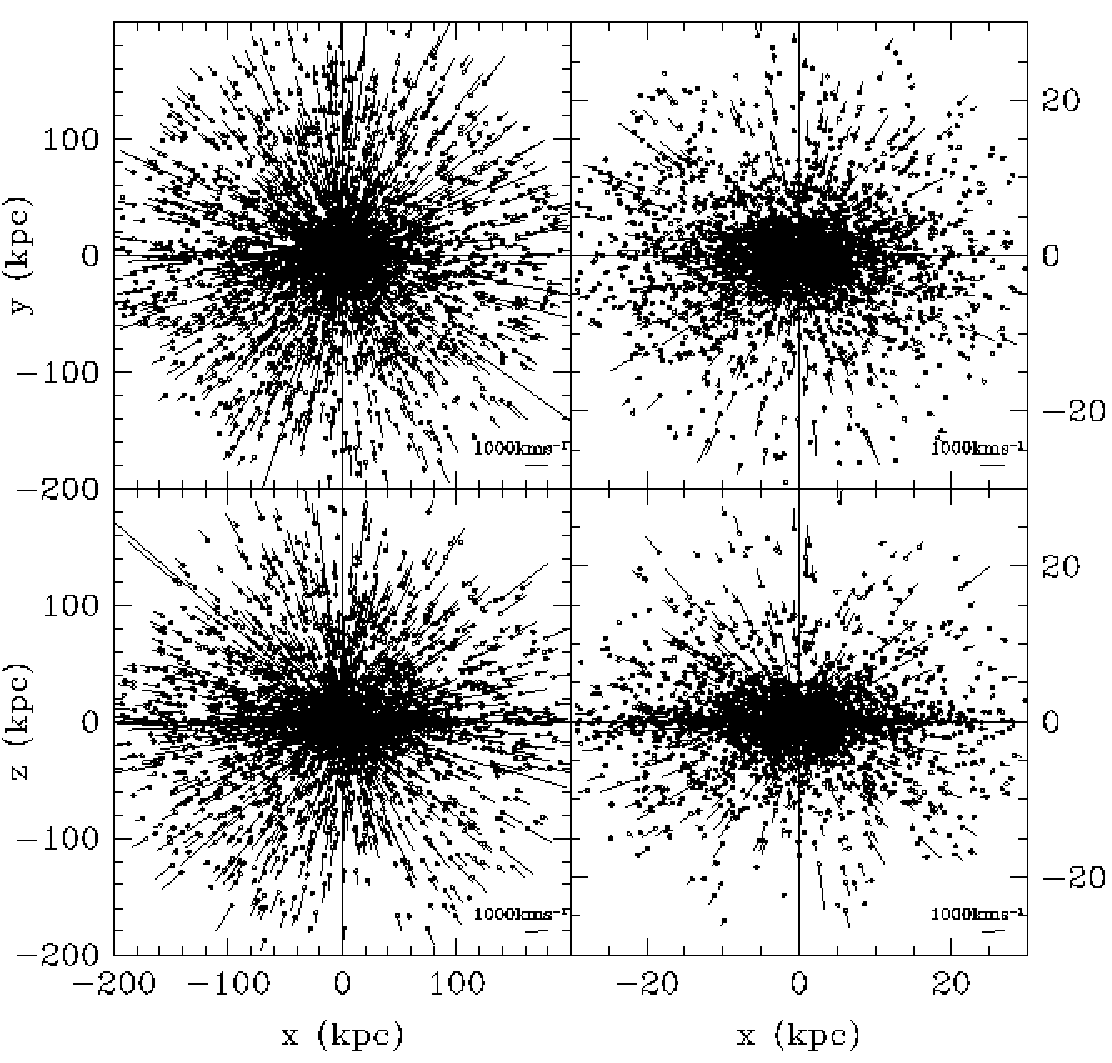
We use the initial conditions described above and numerically integrate the orbits of HVSs in the Galactic potential. Figures 1 and 2 show maps of stellar position and velocity vectors at the present time and their deflection angles . For HVSs with , deviations are quite small, , at all distances within . Lower velocity stars at small distances can instead be bound, and their deflection angles extend to . Many of the stars with and in Figure 2(a) follow bound trajectories, while no stars in this velocity range have substantial deviation angles at large Galactocentric distances. One example of a bound orbit is shown in Figure 3, where the trajectory has been significantly bent by the triaxial halo and the flattened disk potentials, and the star does not return to the Galactic center. Note that bound stars with and large ’s are typically observed at smaller distances () than bound stars of lower velocities. This is because a larger ejection speed from the Galactic center is needed to maintain a high velocity at large distances, and such stars may then have either escaped from the halo or not have had sufficient time to come back and show a significant bend in their orbits. (For reference, the local escape speed is about , Smith et al. 2006.) We find that 60% of the stars with at have velocities , and 20% of the stars with at have velocities .

Figure 5 shows that bound stars with large deflection angles ( have generally traveled a long time after ejection (50 Myr for ), and many of them have experienced at least one orbital period (Fig. 3). HVSs with small deflections () have instead a short travel time and are generally on the initial phases of their first orbital periods (see the concentration of the stars at the left bottom of the panels in Figure 5). The transverse velocities (in the Galactocentric frame) of stars with are typically higher than , and can be up to (hundreds of ) for unbound (bound) HVSs. Note that corresponds at a distance of 100 kpc to a proper motion of as in three years, which can be resolved by the next generation of astrometric surveys like GAIA. According to our calculations most HVSs would have transverse velocities even in the case of a weakly triaxial halo with : these transverse velocities are larger than those associated with the bending of stellar trajectories caused by the axisymmetric disk (see Fig. 2h).
A comparison between Figures 2(e)–(g) and 2(a)–(c) shows that the distribution of deflection angles versus distance is different for trajectories in a spherical rather than triaxial halo. In Figure 2(e) and (f), the angles of bound stars are clustered around and because their orbits are highly eccentric with little bending (see also Fig. 4). By contrast, in Figure 2(a) and (b) the deflection angles of bound stars lies at intermediate values. This difference can be used as an indicator of the triaxiality of the MW dark matter halo.

Figure 6(a)–(c) depicts the values of and versus distance of all the HVSs plotted in Figure 1 having and far from the plane of the disk, i.e. with . Figure 6(d) shows all stars with in the range –. As seen in Figure 6(a), the ratio at large distances () is close to the triaxiality of the halo potential (, solid line) assumed in our calculations, with only a small scatter. The scatter is larger in the quantity plotted in Figure 6(b). The slight offset () of the stellar dots from the solid line is partly due to the disk potential that causes an additional bending of stellar trajectories towards the disk plane, increasing without changing (see the Appendix for details about the correction of such offset owing to the Galactic disk). As shown in Figure 6(e), HVSs become better tracers of triaxiality after removing the disk potential from our calculations. The higher the velocities, the smaller the offset. The curvature of the ratio towards smaller values at small distances is also an effect of the disk. The ratio for stars close to disk plane is not a good approximation of halo triaxiality even at large distances (see Fig. 6d). We plot the values of versus in Figure 7, where Panel (a) shows stars with , and Panel (b) stars with in the full range –. The effect of the disk potential can be seen in the spreading of the stellar dots from the solid line to the dashed line . Note that the scatter in the ratio increases significantly if the reference frame is different from the frame of the triaxial halo potential (Fig. 6f).
5 Summary
We have studied the unique kinematics of HVSs ejected from the Galactic center with almost zero initial specific angular momentum. HVSs can travel in the Galactic halo on either bound or unbound orbits, and their spatial and velocity distribution at large Galactocentric distances () contain information on the asphericity of the halo gravitational potential. We have proposed an estimator of the triaxiality of the Galactic dark matter halo that is determined solely by instantaneous position and velocity vectors of HVSs, is independent of the details of the ejection mechanism, and does not require an accurate knowledge of halo mass. Future astrometric and deep wide-field surveys of HVSs should detect significant numbers of HVSs, which could be used to determine the triaxiality of the MW halo by applying the method proposed in this paper.
The new class of possibly bound HVSs with velocities recently observed by Brown et al. 2007 has Galactocentric distances in the range 30-60 or 10-20 depending on whether they are main-sequence or blue horizontal branch stars. In the first case (main-sequence stars at large distances), they have a lifetime of and are, according to Figure 5, on the initial phases of their first orbital periods. Their deflection angles are expected to be rather small, supporting the fact that a significant excess of B-type stars is observed only at large positive velocities (Brown et al. 2007). If bound HVSs are blue horizontal branch stars instead at smaller distances, the travel time of the stars can be much longer than as at the ejection moment the stars may not necessarily be blue horizontal branch stars but at some pre-blue-horizontal-branch stage. Such stars may have experienced at least one orbital period, and many of them should be returning to the Galactic center or their orbits should have been significantly bent by the asymmetric Galactic potential (Fig. 5). This scenario appear unlikely since it does not agree with the observed positive radial velocities.
It is interesting at this stage to provide an example of a statistical estimate of halo triaxiality from a mock sample. Let us assign a measurement error of () to the one-dimensional velocities of all stars in Figure 6(a) having , , and (our error analysis assumes that the distances to HVSs are known to within ten percent). We have simulated the observed velocities of such a sample, and plot in the top panel of Figure 8 the values of and derived for each HVS. Using equations (12) and (13), we obtain and . For , we obtain and . These errors are comparable with the systematic error caused by the flattened disk (see the slight offset of dots from the solid line in Fig. 6a). We have tried different values of the gravitational potential parameters in the calculations, and found that the estimated value of is always consistent with the assumed halo triaxiality (see middle and bottom panels in Fig. 8).


If the -axis of the halo potential form an angle (measured counter-clockwise) with the reference axis of the observations, then (as seen from Fig. 9) the minimum variance of in a set of simulated samples each in a frame at angle from the observational reference axis (see eq. 17) occurs for . Our calculations show that an error of in the estimate of may cause an error of 2% in the estimate of .
Note that the axis ratios of the halo potential are degenerate in the defined triaxiality parameter (eq. 9). After determining , the values of could be also obtained by using any value of (e.g., see Fig. 6b), but the modeling would be sensitive to halo mass and the shape of halo potential used (see also the determination of axis ratios in Gnedin et al. 2005 by tracing back HVS orbits).
Finally, it is possible that a few HVSs in the halo may be produced by the interactions of stars with an IMBH in satellite galaxies like the Large Magellanic Cloud (Edelmann et al. 2005; Gualandris & Portegies Zwart 2007), and that these would contaminate the sample ejected from the Galactic center. The ejection rates from the satellite dwarfs of the MW are expected to be much smaller than the rate from Sgr A∗, however. Such “satellite” HVSs will also have much larger angular momenta in the Galactocentric rest-frame, and should be easily distinguishable from the Galactic center sample.
We have benefited from discussions with Francesco Haardt, Youjun Lu, and Scott Tremaine. We thank Alberto Sesana for providing the initial velocity and spatial distributions of HVSs ejected from a black hole binary. P.M. acknowledges financial support from NASA through grants NAG5-11513 and NNG04GK85G, and from the Alexander von Humboldt Foundation. Q.Y. acknowledges initial support from NASA through Hubble Fellowship grant HST-HF-01169.01-A awarded by the Space Telescope Science Institute, which is operated by the Association of Universities for Research in Astronomy, Inc., for NASA, under contract NAS 5-26555.
Appendix A Correction of the effect of disk potential on the inferred halo triaxiality
As shown in Figure 6(a), the triaxiality obtained through has a small offset from the true halo triaxiality. Part of this offset comes from the effects of the flattened disk potential, and part from the fixing of in the integration of equation (10). The offset due to the constant assumption is smaller for stars of higher velocities, as seen in Figure 6(e) that shows the results after the disk potential was removed. Below we provide a method to correct the offset due to the Galactic disk. As in the determination of halo triaxiality proposed in this work, even for this correction it is not necessary to trace back the orbits of HVSs.
The contribution to the change in specific angular momentum due to the disk potential can be expressed as:
| (26) |
where
| (27) |
| (28) |
is the initial distance of the HVS from the Galactic center at ejection, and are the current position and velocity of the HVS, , and is its radial velocity at . We can remove the effect of the disk potential from the variable by computing , where
| (29) | |||||
and where equation (20) describing the disk potential has been used. The angles are fixed in the integration to be present-day values. In addition to the disk potential, we also need to assume a halo potential to determine , for which we may use the spherical part of the halo potential by setting . We have tested this correction and found that half of the offset to the true halo triaxiality can be corrected.
References
- Baumgardt et al. (2006) Baumgardt, H., Gualandris, A., & Portegies Zwart, S. 2006, MNRAS, 372, 174
- Begelman, Blandford & Rees (1980) Begelman, M. C., Blandford, R. D., & Rees, M. J. 1980, Nature, 287, 307
- Bromley et al. (2006) Bromley, B. C., Kenyon, S. J., Geller, M. J., Barcikowski, E. B., Warren, R., & Kurtz, M. J. 2006, ApJ, 653, 1194
- Brown et al. (2005) Brown, W. R., Geller, M. J., Kenyon, S. J., & Kurtz, M. J. 2005, ApJ, 622, L33
- Brown et al. (2006a) Brown, W. R., Geller, M. J., Kenyon, S. J., & Kurtz, M. J. 2006a, ApJ, 640, L35
- Brown et al. (2006b) Brown, W. R., Geller, M. J., Kenyon, S. J., & Kurtz, M. J. 2006b, ApJ, 647, 303
- Brown et al. (2007) Brown, W. R., Geller, M. J., Kenyon, S. J., Kurtz, M. J., & Bromley, B. C. 2007, ApJ, in press (astro-ph/0701600)
- Buote et al. (2002) Buote, D. A., Jeltema, T. E., Canizares, C. R., & Garmire, G. P. 2002, ApJ, 577, 183
- Diemand et al. (2007) Diemand, J., Kuhlen, M., & Madau, P. 2007, ApJ, 657, 262
- Dubinski (1994) Dubinski, J. 1994, ApJ, 431, 617
- Edelmann et al. (2005) Edelmann, H., Napiwotzki, R., Heber, U., Christlieb, N., & Reimers, D. 2005, ApJ, 634, L181
- Eisenhauer et al. (2005) Eisenhauer, F., et al. 2005, ApJ, 628, 246
- Ghez et al. (2005) Ghez, A. M., et al. 2005, ApJ, 620, 744
- Ginsburg & Loeb (2006) Ginsburg, I., & Loeb, A. 2006, MNRAS, 368,221
- Gnedin et al. (2005) Gnedin, O. Y., Gould, A., Miralda-Escudé, J., & Zentner, A. R. 2005, ApJ, 634, 344
- Gualandris & Portegies Zwart (2007) Gualandris, A., & Portegies Zwart, S. 2007, MNRAS, in press (astro-ph/0612673)
- Hayashi et al. (2006) Hayashi, E., Navarro, J. F., & Springel, V. 2006, MNRAS, in press (astro-ph/0612327)
- Helmi (2004) Helmi, A. 2004, MNRAS, 351, 643
- Hernquist (1990) Hernquist, L. 1990, ApJ, 356, 359
- Hills (1988) Hills, J. G. 1988, Nature, 331, 687
- Hirsch et al. (2005) Hirsch, H. A., Heber, U., O’Toole, S. J., & Bresolin, F. 2005, A&A, 444, L61
- Hoekstra et al. (2004) Hoekstra, H., Yee, H. K. C., & Gladders, M. D. 2004, ApJ, 606, 67
- Ibata et al. (2001) Ibata, R., Lewis, G. F., Irwin, M., Totten, E., & Quinn, T. 2001, ApJ, 551, 294
- Jing & Suto (2002) Jing, Y. P., & Suto, Y. 2002, ApJ, 574, 538
- Kazantzidis et al. (2004) Kazantzidis, S., Kravtsov, A. V., Zentner, A. R., Allgood, B., Nagai, D., & Moore, B. 2004, ApJ, 611, L73
- Klypin et al. (1999) Klypin, A. A., Kravtsov, A. V., Valenzuela, O., & Prada, F. 1999, ApJ, 630, L141
- Levin (2006) Levin, Y. 2006, ApJ, 653, 1203
- Miyamoto & Nagai (1975) Miyamoto, M., & Nagai, R. 1975, PASJ, 27, 533
- Moore et al. (1999) Moore, B., Ghigna, S., Governato, F., Lake, G., Quinn, T., Stadel, J., & Tozzi, P. 1999, ApJ, 524, L19
- Moore et al. (2004) Moore, B., Kazantzidis, S., Diemand, J., & Stadel, J. 2004, MNRAS, 354, 522
- Navarro et al. (1996) Navarro, J. F., Frenk, C. S., & White, S. D. M., 1996, ApJ, 462, 563
- O’Leary & Loeb (2006) O’Leary, R. M., & Loeb, A. 2006, MNRAS, submitted (astro-ph/0609046)
- Quinlan (1996) Quinlan, G. D. 1996, New Astron., 1, 35
- Sesana et al. (2006) Sesana, A., Haardt, F., & Madau, P. 2006, ApJ, 651, 392
- Sesana et al. (2007) Sesana, A., Haardt, F., & Madau, P. 2007, ApJ, in press (astro-ph/0612265)
- Smith et al. (2006) Smith, M. C., et al. 2006, MNRAS, submitted (astro-ph/0611671)
- Yu (2002) Yu, Q. 2002, MNRAS, 331, 935
- Yu & Tremaine (2003) Yu, Q., & Tremaine, S. 2003, ApJ, 599, 1129
- Zier & Biermann (2001) Zier, C., & Biermann, P. L. 2001, A&A, 377, 23