Ascending number of knots and links
Abstract.
We introduce a new numerical invariant of knots and links from the descending diagrams. It is considered to live between the unknotting number and the bridge number.
Key words and phrases:
knot, link, unknotting number, bridge number, ascending number1991 Mathematics Subject Classification
Primary 57M25; Secondary 57Q351. Introduction
Throughout this paper we work in the piecewise linear category. We shall study knots and links in the three-dimensional Euclidean space . For the standard definitions and results of knots and links, we refer to [1], [2], [3], [6], [10], [11], [12] and [16].
For the purpose of defining a numerical invariant of knots and links, we need to prepare following terms. A link diagram is ordered if an order is given to its components. A link diagram is based if a basepoint (different from the crossing points) is specified on each component. A link diagram is oriented if an orientation is specified on each component.
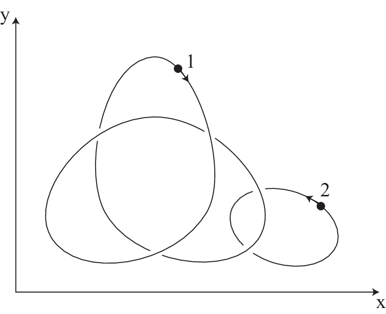
Let be a link, and let be a based ordered oriented link diagram of . The descending diagram of is obtained as follows, and will be denoted by . Beginning at the basepoint of the first component of and proceeding in the direction specified by the orientation, change the crossings as necessary so that each crossing is first encountered as an over-crossing. Continue this procedure with the remaining components in the sequence determined by the ordering, proceeding from the basepoint in the direction determined by the orientation, changing crossings so that ultimately every crossing is first encountered as an over-crossing. The result is the descending diagram obtained from . An example is shown in Figure 1. Note that is a diagram of a trivial link.
 |
 |
Prof. Shin’ichi Suzuki mentioned in [18, 2.16 (ii)] that the smallest number of crossing changes to obtain the trivial link may not always be provided with the number of difference crossing between a link diagram and the descending diagram. That was why we defined the next numerical invariant in [14].
Definition 1.1.
Let be a link and let be a based ordered oriented link diagram of . The ascending number of is defined as the number of different crossings between and , and denoted by . The ascending number of is defined as the minimum number of over all based ordered oriented link diagram of , and denoted by .
The definition and the above note imply that , where denotes the unknotting number of . Accordingly is a trivial link if and only if . A difference of and can become no matter how big. Actually, the mention of S. Suzuki will be demonstrated in Corollary 2.3.
Now this paper is organized as follows. In section 2 we state all results. In section 3 we give all proofs of the results. In section 4 we show a table of the ascending number, the unknotting number, and the bridge number of prime knots with eight crossings or less.
2. Results
Proposition 2.1.
For a nontrivial knot , we have
For a link , we have
where denotes the minimum crossing number of , and denotes the greatest integer which does not exceed .
The following theorem is the fundamental inequality between the ascending number and the bridge number.
Theorem 2.2.
For an -component link , we have
where is the bridge number of .
The following corollary asserts the difference between and .
Corollary 2.3.
For any nonnegative integer , there is a knot such that .
For the connected sum, we have the following proposition.
Proposition 2.4.
For a knot, the ascending number is subadditive with respect to connected sum #, i.e.
It is natural to ask whether the ascending number is additive with respect to the connected sum.
Conjecture 2.5.
For any knots ,
The following corollary solves the above question partially.
Corollary 2.6.
Let be a knot. If satisfies , then
In consequence of this, we have the following corollary.
Corollary 2.7.
For any nonnegative integer , there is a knot such that .
The following theorem characterizes the ascending number one link. We note that Tat Sang Fung ([5]) also obtained the same result for knot case. In fact, he showed that almost descending knots, i.e. knots with diagrams descending except at one crossing, are twist knots.
Theorem 2.8.
Let be an -component link. Then the ascending number of is one if and only if is
| or | ||||
where denotes the split union, and denotes an -component trivial link.
In paticular, the ascending number of a knot is one if and only if is a twist knot.
The following theorem determines the ascending number for torus knots.
Theorem 2.9.
Let and be coprime positive integers, and let be a -torus knot. Then we have
3. Proofs
Proof.
(of Proposition 2.1) At the beginning, we prove the proposition for a link. Let be a link, and let be a based ordered oriented link diagram of with minimum crossings. Consider a based ordered oriented link diagram which is obtained by reversing the order and the orientation of , and let it be denoted by . Then it holds that . Indeed is obtained by reflecting in the plane. Hence
Next we prove the proposition for a knot. Let be a knot, and let be a knot diagram of with minimum crossings. Choose a crossing of and specify a basepoint and an orientation on in the following fashion. Whenever we begin the basepoint of and proceed in the direction specified by the orientation, we first encounter the crossing as an over-crossing.
On the other hand let be a based oriented knot diagram which is obtained by reversing the orientation of and sliding the base point of , as follows. Whenever we begin the basepoint of and proceed in the direction specified by the orientation, we first encounter the crossing as an over-crossing. See Figure 2.
 |
 |
Then it holds that . Indeed a knot consists of a single circle. Hence
This completes the proof. ∎
Proof.
(of Theorem 2.2) Let be a based ordered oriented link diagram of satisfying .
First, we make an -bridge presentation of a trivial link from the descending diagram by isotoping on -coordinate so that satisfy the next conditions. We note that a similar presentation can be seen in [1, Section 3.1].
- (1)
For each , is parametrized by an embedding so that the orientation and basepoint of are in consistency with that of , where denotes the projection .
- (2)
For any such that , , where denotes the hight function .
- (3)
For each , .
- (4)
For each , and are connected by a vertical arc contained in base point of . Thus,
Next, we deform to obtain an -bridge presentation of as follows. Let be the set of crossings of which are different from that of . For each crossing , we isotope the corresponding under-crossing of to exceed the corresponding over-crossing. Here, we may assume that such an operation accrues exactly one maximal point. As a result, we obtain a presentation of whose bridge number is equal to . Figure 3 shows a realization of and in Figure 1.
 |
 |
Hence we have
This arrives at the inequality of Theorem 2.2. ∎
Proof.
(of Corollary 2.3) We will show that a composite knot which is a connected sum of ’s satisfies the inequality of Corollary 2.3. It is known that and . By Schubert’s formula ([17]),
Since an inequality generally holds,
Proof.
(of Proposition 2.4) Let and be based oriented diagram of knots and such that for . By considering diagrams on the 2-sphere, we may assume that basepoints of and are in regions containing a point at infinity. Then we perform a connected sum and to obtain a based oriented diagram as Figure 4.

Therefore
∎
Proof.
Proof.
Proof.
(of Theorem 2.8) The ascending number of the Hopf link is obviously equal to 1. The ascending number of a twist knot is also equal to 1 by the transformation in Figure 5.

Conversely, suppose that and let be a based ordered oriented diagram of with . Then there is just one crossing of that is a difference between and . We make an -bridge presentation of a trivial link from the descending diagram and deform to obtain an -bridge presentation of in the same way as the proof of Theorem 2.2.
There are two cases.
- (1)
The crossing consists of an over-crossing and an under-crossing of .
- (2)
The crossing consists of an over-crossing of and an under-crossing of .
In Case 1, is completely splittable and by a deformation in Figure 6, is a twist knot. Here, we may assume that a basepoint of is in the left most by considering a diagram on the 2-sphere.

In Case 2, is a split union of a Hopf link and -component trivial link by a deformation in Figure 7.

This completes the proof of Theorem 2.8. ∎
Proof.
(of Theorem 2.9) Let be coprime positive integers , a -torus knot and a standard diagram with -crossings.
We assign a basepoint and an orientation to so that whenever we begin the basepoint and proceed by the orientation, we first encounter -crossings as over-crossings. We denote a resultant based oriented diagram by (Figure 8).
On the other hand, let be a based oriented diagram which is obtained by reversing the orientation of and sliding the base point of so that whenever we begin the basepoint of and proceed by the orientation, we first encounter the same -crossings as over-crossings (Figure 8).

Then, it holds that . Hence
4. Table of the ascending number of knots
Here we present a table of the ascending number, unknotting number and bridge number of knots with -crossings or less. The unknotting numbers are cited from [18] except for from [15, Corollary 1.2] and from an unpublished result by J. R. Rickard ([9], [7]). The bridge numbers are cited from [12]. For the ascending numbers, was determined by Miki Okuda ([13]), was determined by Sachie Fujimura ([4]) and she also pointed out , where they belong to Laboratory of Prof. Takao Matumoto, Department of Mathematics, School of Science, Hiroshima University. Miki Okuda also determined , , , , and .
| 1 | 1 | 2 | |
| 1 | 1 | 2 | |
| 2 | 2 | 2 | |
| 1 | 1 | 2 | |
| 1 | 1 | 2 | |
| 2 | 1 | 2 | |
| 2 | 1 | 2 |
| 3 | 3 | 2 | |
| 1 | 1 | 2 | |
| 2 | 2 | 2 | |
| 2 | 2 | 2 | |
| 2 | 2 | 2 | |
| 2 | 1 | 2 | |
| 2 | 1 | 2 |
| 1 | 1 | 2 | |
| 2 or 3 | 2 | 2 | |
| 2 | 2 | 2 | |
| 2 | 2 | 2 | |
| 2 or 3 | 2 | 3 | |
| 2 | 2 | 2 | |
| 2 or 3 | 1 | 2 | |
| 2 | 2 | 2 | |
| 2 or 3 | 1 | 2 | |
| 2 or 3 | 2 | 3 |
| 2 | 1 | 2 | |
| 2 | 2 | 2 | |
| 2 | 1 | 2 | |
| 2 | 1 | 2 | |
| 2 | 2 | 3 | |
| 2 or 3 | 2 | 3 | |
| 2 or 3 | 1 | 3 | |
| 2 | 2 | 2 | |
| 3 | 3 | 3 | |
| 2 | 1 | 3 | |
| 2 | 1 | 3 |
We present a based oriented knot diagram which gives the minimal ascending number. We omit knot diagrams which are same as minimal crossing diagram. As S. Suzuki remarked in [18, 2.16 (i)], the minimal ascending diagram is not unique.
![[Uncaptioned image]](0705.3337v1/5_2.png) |
![[Uncaptioned image]](0705.3337v1/6_1.png) |
![[Uncaptioned image]](0705.3337v1/7_2.png) |
![[Uncaptioned image]](0705.3337v1/7_3.png) |
![[Uncaptioned image]](0705.3337v1/7_4.png) |
![[Uncaptioned image]](0705.3337v1/7_5.png) |
![[Uncaptioned image]](0705.3337v1/7_6.png) |
![[Uncaptioned image]](0705.3337v1/8_1.png) |
![[Uncaptioned image]](0705.3337v1/8_3.png) |
![[Uncaptioned image]](0705.3337v1/8_4.png) |
![[Uncaptioned image]](0705.3337v1/8_6.png) |
![[Uncaptioned image]](0705.3337v1/8_8.png) |
![[Uncaptioned image]](0705.3337v1/8_11.png) |
![[Uncaptioned image]](0705.3337v1/8_12.png) |
![[Uncaptioned image]](0705.3337v1/8_13.png) |
![[Uncaptioned image]](0705.3337v1/8_14.png) |
![[Uncaptioned image]](0705.3337v1/8_15.png) |
|
Acknowledgement. I would like to thank Ryo Nikkuni for informimg me a result of Tat Sang Fung about Theorem 2.8.
References
- [1] C. Adams, The Knot Book, American Mathematical Society, 2004.
- [2] G. Burde and H. Zieschang, Knots, Walter de Gruyter, 2002.
- [3] P. Cromwell, Knots and Links, Cambridge University Press, 2004.
- [4] S. Fujimura, On the ascending number of knots, a thesis, Hiroshima University, 1998.
- [5] T. S. Fung, Immersions in knot theory, a dissertation, Columbia University, 1996.
- [6] A. Kawauchi, Survey on Knot Theory, Birkhäuser Verlag, 1996.
- [7] R. Kirby, Problems in low-dimensional topology, Geometric Topology 2, Amer. Math. Soc., (1997) 35-473.
- [8] P. B. Kronheimer and T. S. Mrowka, Gauge theory for embedded surfaces, Topology 32 (1993) 773-826.
- [9] W. B. R. Lickorish, The unknotting number of a classical knot, Contemp. Math. 44 (1985) 117-121.
- [10] W. B. R. Lickorish, An Introduction to Knot Theory, Springer, 1997.
- [11] C. Livingston, Knot Theory, The Mathematical Association of America, 1996.
- [12] K. Murasugi, Knot Theory and Its Applications, translated by B. Kurpita, Birkhäuser Boston, 1996.
- [13] M. Okuda, A determination of the ascending number of some knots, a thesis, Hiroshima University, 1998.
- [14] M. Ozawa, Ascending number of knots and links, a talk in a conference “Knot Theory” at Waseda University, 1995.
- [15] P. Ozsvath and Z. Szabo, Knots with unknotting number one and Heegaard Floer homology, Topology 44 (2005) 705-745.
- [16] D. Rolfsen, Knots and Links, AMS Chelsea Publishing, 2003.
- [17] H. Schubert, Über eine numerische Knoteninvariante, Math. Z. 61 (1954) 245-288.
- [18] S. Suzuki, An introduction to knot theory, Saiensu-sha Co., Ltd. Publishers, 1991.