跳到论文正文
W Papers独立论文阅读器 arXiv:0705.3271 论文正文 计算阅读时间 · 0%
引用这篇论文根据当前论文元数据生成,正式投稿前建议核对。


License: Assumed arXiv.org perpetual non-exclusive license
arXiv:0705.3271v1 [math.GT] 23 May 2007

Billiards in L-shaped tables with barriers

Matt Bainbridge
Abstract

We compute the volumes of the eigenform loci in the moduli space of genus two Abelian differentials. From this, we obtain asymptotic formulas for counting closed billiards paths in certain L-shaped polygons with barriers.

1 Introduction

Let P=P⁡(a,b,t)P=P(a,b,t) be the L-shaped polygon with barrier shown in Figure 1. A billiards path on PP is a path which is geodesic on int⁡(P)\interior(P) and which bounces off of the sides of PP so that the angle of incidence equals the angle of reflection. We allow billiards paths to pass through one of the six corners of PP but not through the endpoint pp of the barrier. A saddle connection is a billiards path which joins pp to itself. Each periodic billiards path is contained in a family of parallel periodic billiards paths called a cylinder, and each cylinder is bounded by a union of saddle connections. A saddle connection is proper if it does not bound a cylinder. We say that a saddle connection is multiplicity one if it passes through a corner and multiplicity two otherwise.

We define the following counting functions:

Nc​(P,L)=\displaystyle N_{\rm c}(P,L)= #​{maximal cylinders of length at most L},\displaystyle\#\{\text{maximal cylinders of length at most $L$}\},
Ns1​(P,L)=\displaystyle N_{\rm s}^{1}(P,L)= #​{proper multiplicity one saddle connections of length at most L},\displaystyle\#\{\text{proper multiplicity one saddle connections of length at most $L$}\},
Ns2​(P,L)=\displaystyle N_{\rm s}^{2}(P,L)= #​{proper multiplicity two saddle connections of length at most L}.\displaystyle\#\{\text{proper multiplicity two saddle connections of length at most $L$}\}.

Note that we are counting unoriented saddle connections and cylinders, and we do not count periodic paths which repeat more than once.

In this paper, we will show:

Theorem 1.1.

Consider the polygon P=P⁡(x+z​d,y+z​d,t)P=P(x+z\sqrt{d},y+z\sqrt{d},t), with t>0t>0, x,y,z∈ℚx,y,z\in{\mathbb{Q}}, x+y=1x+y=1, d∈ℕd\in{\mathbb{N}} nonsquare, and

P≠P⁡(1+52,1+52,5−510).P\neq P\left(\frac{1+\sqrt{5}}{2},\frac{1+\sqrt{5}}{2},\frac{5-\sqrt{5}}{10}\right). (1.1)

We have the following asymptotics:

Nc​(P,L)\displaystyle N_{\rm c}(P,L) ∼152​π​Area⁡(P)​L2,\displaystyle\sim\frac{15}{2\pi\Area(P)}L^{2},
Ns1​(P,L)\displaystyle N_{\rm s}^{1}(P,L) ∼2716​Area⁡(P)​π​L2,and\displaystyle\sim\frac{27}{16\Area(P)}\pi L^{2},\quad\text{and}
Ns2​(P,L)\displaystyle N_{\rm s}^{2}(P,L) ∼516​Area⁡(P)​π​L2.\displaystyle\sim\frac{5}{16\Area(P)}\pi L^{2}.
Remark.

The notation a⁡(L)∼b⁡(L)a(L)\sim b(L) means a⁡(L)/b⁡(L)→1a(L)/b(L)\to 1 as L→∞L\to\infty.

Figure 1: P⁡(a,b,t)P(a,b,t)

Using [Vee89], one can show for the surface PP of (1.1),

Nc​(P,L)\displaystyle N_{\rm c}(P,L) ∼7516​π​Area⁡(P)​L2,\displaystyle\sim\frac{75}{16\pi\Area(P)}L^{2},
Ns1​(P,L)\displaystyle N_{\rm s}^{1}(P,L) ∼1125+425​5128​π​Area⁡(P)​L2,and\displaystyle\sim\frac{1125+425\sqrt{5}}{128\pi\Area(P)}L^{2},\quad\text{and}
Ns2​(P,L)\displaystyle N_{\rm s}^{2}(P,L) ∼125−25​532​π​Area⁡(P)​L2.\displaystyle\sim\frac{125-25\sqrt{5}}{32\pi\Area(P)}L^{2}.

Spaces of Abelian differentials.

There is an unfolding construction which associates to a rational angled polygon PP a Riemann surface XX equipped with an Abelian differential (holomorphic 1-form) ω\omega. The unfolding (X,ω)(X,\omega) consists of several reflected copies of PP glued along their boundaries. One step in the proof of Theorem 1.1 is the computation of the volumes of certain spaces of Abelian differentials in which the unfoldings of the polygons P⁡(a,b,t)P(a,b,t) lie. These volume computations are the focus of this paper.

More precisely, let Ω1​ℳ2\Omega_{1}{\mathcal{M}}_{2} be the moduli space of genus two Abelian differentials (X,ω)(X,\omega) such that ∫X|ω|2=1\int_{X}|\omega|^{2}=1, and let Ω1​ℳ2​(1,1)\Omega_{1}{\mathcal{M}}_{2}(1,1) be the locus of differentials with two simple zeros. Given a square-free D∈ℕD\in{\mathbb{N}} with D≡0D\equiv 0 or 1(mod4)1\pmod{4}, let

Ω1​ED⊂Ω1​ℳ2\Omega_{1}E_{D}\subset\Omega_{1}{\mathcal{M}}_{2}

be the locus of eigenforms for real multiplication of discriminant DD (we discuss real multiplication in §4), and let Ω1​ED​(1,1)=Ω1​ED∩Ω1​ℳ2​(1,1)\Omega_{1}E_{D}(1,1)=\Omega_{1}E_{D}\cap\Omega_{1}{\mathcal{M}}_{2}(1,1). The locus Ω1​ED\Omega_{1}E_{D} is a circle bundle over a Zariski-open subset of the Hilbert modular surface of discriminant DD,

XD=(ℍ×(−ℍ))/SL2​𝒪D,X_{D}=({\mathbb{H}}\times(-{\mathbb{H}}))/{\mathrm{SL}}_{2}\mathcal{O}_{D}, (1.2)

where 𝒪D⊂ℚ⁡(D)\mathcal{O}_{D}\subset{\mathbb{Q}}(\sqrt{D}) is the unique real quadratic order of discriminant DD. The unfolding of the polygon P⁡(a,b,t)P(a,b,t) is genus two. It has two simple zeros if and only if t>0t>0, and it is an eigenform if and only if aa and bb are as in Theorem 1.1.

There is a natural action of SL2​ℝ{\mathrm{SL}}_{2}{\mathbb{R}} on Ω1​ℳ2\Omega_{1}{\mathcal{M}}_{2} which preserves the spaces Ω1​ℳ2​(1,1)\Omega_{1}{\mathcal{M}}_{2}(1,1) and Ω1​ED\Omega_{1}E_{D}. There is a natural absolutely continuous, finite, ergodic SL2​ℝ{\mathrm{SL}}_{2}{\mathbb{R}}-invariant measure μD1\mu_{D}^{1} on Ω1​ED\Omega_{1}E_{D} which is constructed in [McM07a]. The main result of this paper is that the volume of Ω1​ED\Omega_{1}E_{D} with respect to this measure is proportional to the orbifold Euler characteristic of XDX_{D}:

Theorem 1.2.

The μD1\mu_{D}^{1}-volume of Ω1​ED\Omega_{1}E_{D} is 4​π​χ​(XD)4\pi\chi(X_{D}).

Remark.

This theorem was conjectured by Maryam Mirzakhani.

From a formula of Siegel for χ⁡(XD)\chi(X_{D}), we obtain the explicit formula:

vol⁡Ω1​Ef2​D=8​π​f3​ζℚ⁡(D)​(−1)​∑r|f(Dr)​μ⁡(r)r2,\Vol\Omega_{1}E_{f^{2}D}=8\pi f^{3}\zeta_{{\mathbb{Q}}(\sqrt{D})}(-1)\sum_{r|f}\left(\frac{D}{r}\right)\frac{\mu(r)}{r^{2}},

for DD a fundamental discriminant.

Counting functions.

In order to prove Theorem 1.1, we need also to evaluate integrals over Ω1​ED​(1,1)\Omega_{1}E_{D}(1,1) of certain counting functions. A Riemann surface with Abelian differential (X,ω)(X,\omega) carries a flat metric |ω||\omega| on the complement of the zeros of ω\omega. A saddle connection is a geodesic segment joining two zeros of ω\omega whose interior is disjoint from the zeros. If XX is genus two, it has a hyperelliptic involution JJ. We say that a saddle connection II joining distinct zeros has multiplicity one if J⁡(I)=IJ(I)=I, and otherwise it has multiplicity two. As for billiards paths, closed geodesics occur in parallel families forming metric cylinders bounded by saddle connections. We define for T∈Ω1​ℳ2​(1,1)T\in\Omega_{1}{\mathcal{M}}_{2}(1,1):

Nc​(T,L)=\displaystyle N_{\rm c}(T,L)= #​{maximal cylinders on T of circumference at most L},\displaystyle\#\{\text{maximal cylinders on $T$ of circumference at most $L$}\},
Ns1​(T,L)=\displaystyle N_{\rm s}^{1}(T,L)= #{multiplicity one saddle connections on T of length at most L\displaystyle\#\{\text{multiplicity one saddle connections on $T$ of length at most $L$}
joining distinct zeros of T},and\displaystyle\text{joining distinct zeros of $T$}\},\quad\text{and}
Ns2​(T,L)=\displaystyle N_{\rm s}^{2}(T,L)= #{pairs of multiplicity two saddle connections on T of length at\displaystyle\#\{\text{pairs of multiplicity two saddle connections on $T$ of length at}
most L joining distinct zeros of T}.\displaystyle\text{most $L$ joining distinct zeros of $T$}\}.

We will show in §11:

Theorem 1.3.

For any L>0L>0,

∫Ω1​ED​(1,1)Nc​(T,L)​d​μD1​(T)\displaystyle\int\limits_{\Omega_{1}E_{D}(1,1)}N_{\rm c}(T,L)\,d\mu_{D}^{1}(T) =60​L2​χ​(XD),\displaystyle=60L^{2}\chi(X_{D}), (1.3)
∫Ω1​ED​(1,1)Ns1​(T,L)​d​μD1​(T)\displaystyle\int\limits_{\Omega_{1}E_{D}(1,1)}N_{\rm s}^{1}(T,L)\,d\mu_{D}^{1}(T) =272​π2​L2​χ​(XD),and\displaystyle=\frac{27}{2}\pi^{2}L^{2}\chi(X_{D}),\quad\text{and} (1.4)
∫Ω1​ED​(1,1)Ns2​(T,L)​d​μD1​(T)\displaystyle\int\limits_{\Omega_{1}E_{D}(1,1)}N_{\rm s}^{2}(T,L)\,d\mu_{D}^{1}(T) =52​π2​L2​χ​(XD).\displaystyle=\frac{5}{2}\pi^{2}L^{2}\chi(X_{D}). (1.5)

Uniform distribution of circles.

Given T∈Ω1​EDT\in\Omega_{1}E_{D}, let mTm_{T} be the measure on Ω1​ED\Omega_{1}E_{D} obtained by transporting the Haar measure on SO2​ℝ{\rm SO}_{2}{\mathbb{R}} to the orbit SO2​ℝ⋅T{\rm SO}_{2}{\mathbb{R}}\cdot T. Let

at=(et00e−t).a_{t}=\begin{pmatrix}e^{t}&0\\ 0&e^{-t}\end{pmatrix}.

The measure (at)∗​mT(a_{t})_{*}m_{T} is the uniform measure on a circle centered at pp in the SL2​ℝ{\mathrm{SL}}_{2}{\mathbb{R}} orbit through pp.

There is a Teichmüller curve Ω1​D10⊂Ω1​E5​(1,1)\Omega_{1}D_{10}\subset\Omega_{1}E_{5}(1,1) which is the SL2​ℝ{\mathrm{SL}}_{2}{\mathbb{R}}-orbit of the Abelian differential obtained by identifying opposite sides of a regular decagon. In §12, we prove

Theorem 1.4.

For any point T∈Ω1​ED​(1,1)T\in\Omega_{1}E_{D}(1,1) which does not lie on the curve Ω1​D10\Omega_{1}D_{10}, we have

limt→∞(at)∗​mT=μD1vol⁡μD1.\lim_{t\to\infty}(a_{t})_{*}m_{T}=\frac{\mu_{D}^{1}}{\Vol\mu_{D}^{1}}. (1.6)

The proof of Theorem 1.4 is a straightforward adaption of an argument in [EMM06] together with a partial classification of ergodic horocycle-invariant measures on Ω1​ED\Omega_{1}E_{D} obtained in [CW].

It follows from [EM01] that if (1.6) holds for T∈Ω1​ED​(1,1)T\in\Omega_{1}E_{D}(1,1), then

N⁡(T,L)∼c​L2,N(T,L)\sim cL^{2},

where

c=1L2​vol⁡(μD1)​∫Ω1​ED​(1,1)Nc​(T,L)​d​μD1​(T),c=\frac{1}{L^{2}\Vol(\mu_{D}^{1})}\int\limits_{\Omega_{1}E_{D}(1,1)}N_{\rm c}(T,L)\,d\mu_{D}^{1}(T),

and similarly for the counting functions from saddle connections.

We then obtain from Theorems 1.2 and 1.3:

Theorem 1.5.

For every T∈Ω1​ED​(1,1)T\in\Omega_{1}E_{D}(1,1) which does not lie on Ω1​D10\Omega_{1}D_{10},

Nc​(T,L)\displaystyle N_{\rm c}(T,L) ∼15π​L2,\displaystyle\sim\frac{15}{\pi}L^{2},
Ns1​(T,L)\displaystyle N_{\rm s}^{1}(T,L) ∼278​π​L2,and\displaystyle\sim\frac{27}{8}\pi L^{2},\quad\text{and}
Ns2​(T,L)\displaystyle N_{\rm s}^{2}(T,L) ∼58​π​L2.\displaystyle\sim\frac{5}{8}\pi L^{2}.

Theorem 1.1 follows directly from this by applying the unfolding construction.

Outline of proof of Theorem 1.2.

The proof of Theorem 1.2 proceeds in the following steps:

  1. 1.

    Let μD\mu_{D} be the projection of μD1\mu_{D}^{1} to XDX_{D}. It is enough to calculate vol⁡(μD)\Vol(\mu_{D}). There is a foliation ℱD\mathcal{F}_{D} of XDX_{D} by hyperbolic Riemann surfaces covered by SL2​ℝ{\mathrm{SL}}_{2}{\mathbb{R}}-orbits on Ω1​ED\Omega_{1}E_{D}. The foliation ℱD\mathcal{F}_{D} has a natural transverse measure which we discuss in §4, and the product of this measure with the leafwise hyperbolic measure is μD\mu_{D}.

  2. 2.

    There is a compactification YDY_{D} of XDX_{D} which we studied in [Bai]. The space YDY_{D} is a complex orbifold, and the boundary ∂XD=YD∖XD\partial X_{D}=Y_{D}\setminus X_{D} is a union of rational curves. These curves are parameterized by numerical invariants called prototypes which we discuss in §5. There is one rational curve CP⊂∂XDC_{P}\subset\partial X_{D} for each prototype PP. We summarize the relevant properties of YDY_{D} in §7.

  3. 3.

    The foliation ℱD\mathcal{F}_{D} doesn’t extend to a foliation of YDY_{D}; however, in §8, we show that integration over the measured foliation ℱD\mathcal{F}_{D} defines a closed current on YDY_{D}. The form,

    ω~1=12​π​d​x1∧d​y1y12,\widetilde{\omega}_{1}=\frac{1}{2\pi}\frac{dx_{1}\wedge dy_{1}}{y_{1}^{2}},

    on ℍ×ℍ{\mathbb{H}}\times{\mathbb{H}} descends to a closed 2-form ω1\omega_{1} on XDX_{D} which also defines a closed current on YDY_{D}. In §8, we also show that

    vol⁡(μD)=[ℱ¯D]⋅[ω1],\Vol(\mu_{D})=[\overline{\mathcal{F}}_{D}]\cdot[\omega_{1}], (1.7)

    where [ℱ¯D][\overline{\mathcal{F}}_{D}] and [ω1][\omega_{1}] are the classes in H2​(YD,ℝ)H^{2}(Y_{D};{\mathbb{R}}) defined by these currents, and the product is the intersection product on cohomology.

  4. 4.

    There are closed leaves WDW_{D} and PDP_{D} of ℱD\mathcal{F}_{D} whose closures are smooth curves in YDY_{D}. From [Bai], we have

    [ω1]=−13​[W¯D]+35​[P¯D]−415​BD,[\omega_{1}]=-\frac{1}{3}[\overline{W}_{D}]+\frac{3}{5}[\overline{P}_{D}]-\frac{4}{15}B_{D},

    where BDB_{D} is a certain linear combination of fundamental classes of the curves CP⊂∂XDC_{P}\subset\partial X_{D}. Thus by (1.7), we need only to compute the intersection numbers of these curves with [ℱ¯D][\overline{\mathcal{F}}_{D}].

  5. 5.

    In §9, we show that

    [W¯D]⋅[ℱ¯D]=[P¯D]⋅[ℱ¯D]=0.[\overline{W}_{D}]\cdot[\overline{\mathcal{F}}_{D}]=[\overline{P}_{D}]\cdot[\overline{\mathcal{F}}_{D}]=0. (1.8)

    Heuristically, these intersection numbers are zero because these curves are leaves of ℱ¯D\overline{\mathcal{F}}_{D}, and a closed, nonatomic leaf of a measured foliation has zero intersection number with that foliation. Since ℱ¯D\overline{\mathcal{F}}_{D} is singular at the cusps of W¯D\overline{W}_{D} and P¯D\overline{P}_{D}, this intersection number is a priori not necessarily zero. However, leaves close to W¯D\overline{W}_{D} or P¯D\overline{P}_{D} tend to diverge from these curves near the cusps, so these cusps should not contribute to the intersection number.

    Here is the idea of the rigorous proof of (1.8): In §2, we construct for any Riemann surface XX a canonical measured foliation 𝒞X\mathcal{C}_{X} of T​XTX by Riemann surfaces and show essentially that the intersection number of the zero section of T​XTX with 𝒞X\mathcal{C}_{X} is zero. In §9, we show that there is a tubular neighborhood of W¯D\overline{W}_{D} or P¯D\overline{P}_{D} which is isomorphic to a neighborhood of the zero section of (a twist of) T​W¯DT\overline{W}_{D} or T​P¯DT\overline{P}_{D}. Furthermore, this isomorphism takes the foliation ℱD\mathcal{F}_{D} to the canonical foliation defined in §2. From this, we obtain (1.8).

  6. 6.

    In §10, we calculate the intersection numbers [ℱ¯D]⋅CP[\overline{\mathcal{F}}_{D}]\cdot C_{P} and obtain Theorem 1.2.

Notation.

Here we fix some notation that we will use throughout this paper. Given a manifold MM equipped with a foliation ℱ\mathcal{F} by hyperbolic Riemann surfaces and a nn-form ω\omega, we will denote by ‖ω‖ℱ\|\omega\|_{\mathcal{F}} the function on MM defined at xx by:

‖ωx‖ℱ=supv1,…,vn∈Tx​ℱ|ω⁡(v1,…,vn)|‖v1​‖⋯‖​vn‖,\|\omega_{x}\|_{\mathcal{F}}=\sup_{v_{1},\dots,v_{n}\in T_{x}\mathcal{F}}\frac{|\omega(v_{1},\dots,v_{n})|}{\|v_{1}\|\cdots\|v_{n}\|}, (1.9)

where the norms of vectors is with respect the hyperbolic metric. Similarly, if hh is a Riemannian metric, then ‖ω‖h\|\omega\|_{h} will denote the analogous norm with the supremum over all vectors tangent MM.

We use the notation x≺yx\prec y to mean that |x|<C​|y||x|<C|y| for an arbitrary positive constant CC. We use x≍yx\asymp y to mean that c<|x/y|<Cc<|x/y|<C for arbitrary positive constants cc and CC, and we say that xx is comparable to yy. We write C⁡(x)C(x) for an arbitrary positive constant depending only on the data xx.

We use the following notation for subsets of ℂ{\mathbb{C}}: ℍ{\mathbb{H}} will denote the upper-half plane, Δr\Delta_{r} the disk of radius rr, and Δr∗=Δr∖{0}\Delta^{*}_{r}=\Delta_{r}\setminus\{0\} the punctured disk.

GL2+​ℝ{\rm GL}_{2}^{+}{\mathbb{R}} denotes the identity component of GL2​ℝ{\rm GL}_{2}{\mathbb{R}}. We write BB for the subgroup of upper-triangular matrices, and HH for the subgroup of BB with ones on the diagonal. We write:

at=(et00e−t),ht=(1t01),andrθ=(cos⁡θ−sin⁡θsin⁡θcos⁡θ).a_{t}=\begin{pmatrix}e^{t}&0\\ 0&e^{-t}\end{pmatrix},\quad h_{t}=\begin{pmatrix}1&t\\ 0&1\end{pmatrix},\quad\text{and}\quad r_{\theta}=\begin{pmatrix}\cos\theta&-\sin\theta\\ \sin\theta&\cos\theta\end{pmatrix}.

Notes and references.

McMullen classified the orbit closures for the action of SL2​ℝ{\mathrm{SL}}_{2}{\mathbb{R}} on Ω1​ℳ2\Omega_{1}{\mathcal{M}}_{2} in the series of papers, [McM06, McM05b, McM05a, McM03b, McM07a, McM03a]. See also [Cal04] and [HL06]. The orbit closures in this classification are the entire space, the stratum Ω1​ℳ2​(2)\Omega_{1}{\mathcal{M}}_{2}(2), the eigenform loci Ω1​ED\Omega_{1}E_{D}, the curves Ω1​WD\Omega_{1}W_{D}, the decagon curve Ω1​D10\Omega_{1}D_{10}, and infinitely many Teichmüller curves generated by square-tiled surfaces. This paper, together with [Bai] almost finishes computing the volumes of all of these orbit closures (see also [LR06]). It only remains to understand the Teichmüller curves generated by square-tiled surfaces with two simple zeros.

There has been much recent work on computing asymptotics for closed geodesics and configurations of saddle connections on rational billiards tables and flat surfaces. It is conjectured for any surface (X,ω)(X,\omega) of any genus,

Nc​((X,ω),L)∼C​L2N_{\rm c}((X,\omega),L)\sim CL^{2}

for some constant CC which depends on (X,ω)(X,\omega). This constant CC is called a Siegel-Veech constant Veech [Vee89] showed quadratic asymptotics for any lattice surface (X,ω)(X,\omega) (this means that the affine automorphism group of (X,ω)(X,\omega) determines a lattice in SL2​ℝ{\mathrm{SL}}_{2}{\mathbb{R}}). He also computed the Siegel-Veech constants for an infinite series of examples obtained by gluing regular nn-gons. Eskin and Masur [EM01], building on work of Veech [Vee98], obtained quadratic asymptotics for almost every Abelian differential (X,ω)(X,\omega) with a given genus and orders of zeros, and [EMZ03] computed the Siegel-Veech constants. Eskin, Masur, and Schmoll [EMS03] evaluated the Siegel-Veech constants for the polygons P⁡(a,b,t)P(a,b,t) of Theorem 1.1 with a,b∈ℚa,b\in{\mathbb{Q}} and t∈ℝ∖ℚt\in{\mathbb{R}}\setminus{\mathbb{Q}} (this case can also be handled with the methods of this paper). See also [GJ00], [Sch05], [EMM06], and [Lel06] for more about Siegel-Veech constants.

I would like to thank Curt McMullen, Maryam Mirzakhani, Alex Eskin, Howard Masur, and Florian Herzig for useful conversations over the course of this work. I am also grateful to IHES for their hospitality during the preparation of this paper.

2 Canonical foliations

In this section, we discuss a canonical measured foliation 𝒞X\mathcal{C}_{X} of the tangent bundle T​XTX of any Riemann surface XX. In the case where XX has finite volume, we study smooth 22-forms on a certain extension LL of the bundle T​XTX over the compactification X¯\overline{X}. We will show that for some compactly supported 2-form Ψ\Psi on LL which represents the Thom class, ∫𝒞XΨ=0\int_{\mathcal{C}_{X}}\Psi=0. These foliated bundles will serve as models for tubular neighborhoods of closed leaves of ℱD\mathcal{F}_{D} and will be used in the proof of (1.8) in §9.

Action of PSL2​ℝ{\rm PSL}_{2}{\mathbb{R}} on ℂ{\mathbb{C}}.

Let QQ be the complex plane ℂ{\mathbb{C}} equipped with the quadratic differential

q=12​z​d​z2.q=\frac{1}{2z}dz^{2}.

Define an action of PSL2​ℝ{\rm PSL}_{2}{\mathbb{R}} on QQ by qq-affine automorphisms as follows. Let SL2​ℝ{\mathrm{SL}}_{2}{\mathbb{R}} act on ℂ{\mathbb{C}} by

(abcd)⋅(x+i​y)=(a​x−b​y)+i⁡(−c​x+d​y).\begin{pmatrix}a&b\\ c&d\end{pmatrix}\cdot(x+iy)=(ax-by)+i(-cx+dy).

Given z∈Qz\in Q, define A∘zA\circ z so that the following diagram commutes,

ℂ\textstyle{{\mathbb{C}}\ignorespaces\ignorespaces\ignorespaces\ignorespaces\ignorespaces\ignorespaces\ignorespaces\ignorespaces}A⋅\scriptstyle{A\cdot}f\scriptstyle{f}ℂ\textstyle{{\mathbb{C}}\ignorespaces\ignorespaces\ignorespaces\ignorespaces}f\scriptstyle{f}Q\textstyle{Q\ignorespaces\ignorespaces\ignorespaces\ignorespaces}A∘\scriptstyle{A\circ}Q\textstyle{Q}

where f⁡(z)=z2f(z)=z^{2}.

Canonical foliations.

Let PSL2​ℝ{\rm PSL}_{2}{\mathbb{R}} act on ℍ{\mathbb{H}} on the left by Möbius transformations in the usual way:

(abcd)⋅z=a​z+bc​z+d,\begin{pmatrix}a&b\\ c&d\end{pmatrix}\cdot z=\frac{az+b}{cz+d},

and give ℍ×Q{\mathbb{H}}\times Q the product action of PSL2​ℝ{\rm PSL}_{2}{\mathbb{R}}. Define Φ:ℍ×Q→T​ℍ\Phi\colon{\mathbb{H}}\times Q\to T{\mathbb{H}} by

Φ⁡(z,(u+i​v)2)=(z,(u+z​v)2​∂∂z).\Phi(z,(u+iv)^{2})=\left(z,(u+zv)^{2}\frac{\partial}{\partial z}\right).

The following lemma is a straightforward calculation:

Lemma 2.1.

Φ\Phi commutes with the PSL2​ℝ{\rm PSL}_{2}{\mathbb{R}} actions on ℍ×Q{\mathbb{H}}\times Q and T​ℍT{\mathbb{H}}.

The map Φ\Phi sends the horizontal foliation of ℍ×Q{\mathbb{H}}\times Q with the transverse measure induced by the quadratic differential qq to a measured foliation of T​ℍT{\mathbb{H}}. Call this measured foliation 𝒞ℍ\mathcal{C}_{\mathbb{H}}.

Let X=Γ\ℍX=\Gamma\backslash{\mathbb{H}} be a hyperbolic Riemann surface, or more generally a hyperbolic Riemann surface orbifold. By Lemma 2.1, the foliation 𝒞ℍ\mathcal{C}_{\mathbb{H}} of T​ℍT{\mathbb{H}} descends to a measured foliation of T​XTX. Call this measured foliation 𝒞X\mathcal{C}_{X}.

Global angular forms.

Let XX be a compact 22-dimensional real orbifold equipped with a line bundle π:L→X\pi\colon L\to X with a Hermitian metric. Given an open set U⊂XU\subset X with a trivialization π−1​(U)→U×ℂ\pi^{-1}(U)\to U\times{\mathbb{C}}, let d​θUd\theta_{U} be the 11-form induced by the standard angular form on ℂ{\mathbb{C}},

d​θ=12​π​x​d​y−y​d​xx2+y2.d\theta=\frac{1}{2\pi}\frac{x\,dy-y\,dx}{x^{2}+y^{2}}.

Choose a compactly supported smooth bump function ρ:[0,∞)→ℝ\rho\colon[0,\infty)\to{\mathbb{R}} with ρ⁡(r)≡1\rho(r)\equiv 1 near 00. Using the Hermitian metric, we regard ρ⁡(r)\rho(r) as a smooth function on LL.

The following theorem follows from the discussion on pp.70-74 of [BT82]:

Theorem 2.2.

There is a smooth 11-form ψ\psi on the complement of the zero section of LL with the following properties:

  • •

    For any contractable domain U⊂XU\subset X, we have on π−1​(U)\pi^{-1}(U),

    ψ=d​θU+π∗​η,\psi=d\theta_{U}+\pi^{*}\eta,

    for some smooth 11-form η\eta on UU.

  • •

    d​ψ=−π∗​e,d\psi=-\pi^{*}e, with ee a smooth 22-form representing the Euler class of LL.

  • •

    Ψ=d⁡(ρ⁡(r)​ψ)\Psi=d(\rho(r)\psi) is a compactly supported smooth 22-form representing the Thom class of LL.

Such a form ψ\psi is called a global angular form for LL.

Intersection of zero section with 𝒞X\mathcal{C}_{X}.

Now, consider the following situation. Let X=Γ\ℍX=\Gamma\backslash{\mathbb{H}} be a finite volume hyperbolic orbifold and X¯\overline{X} its compactification. Let

L=TX¯(−∑ci),L=T\overline{X}\left(-\sum c_{i}\right),

where the cic_{i} are the cusps of XX. That is, LL is the line bundle whose nonzero holomorphic sections are holomorphic sections of T​X¯T\overline{X} which have simple zeros at the cusps cic_{i}. Equip LL with a Hermitian metric hh. Let ψ\psi be a global angular form on LL and let Ψ=d⁡(ρ⁡(r)​ψ)\Psi=d(\rho(r)\psi).

Theorem 2.3.

With XX and Ψ\Psi as above,

∫𝒞XΨ=0.\int_{\mathcal{C}_{X}}\Psi=0.

The proof will follow a series of lemmas.

Lemma 2.4.

For any smooth, compactly supported form η\eta on LL, ‖η‖𝒞X≺1\|\eta\|_{\mathcal{C}_{X}}\prec 1.

Proof.

Since η\eta is a smooth form on LL, it suffices to bound ‖η‖𝒞X\|\eta\|_{\mathcal{C}_{X}} over a neighborhood of each cusp. Suppose cc is a cusp of X=Γ\ℍX=\Gamma\backslash{\mathbb{H}}, and conjugate Γ\Gamma so that c=i​∞c=i\infty and Stab∞⁡Γ\Stab_{\infty}\Gamma is generated by z↦z+2​πz\mapsto z+2\pi.

Identify T​ℍT{\mathbb{H}} and ℍ×ℂ{\mathbb{H}}\times{\mathbb{C}} by

(z,t)↦(z,t​∂∂z).(z,t)\mapsto\left(z,t\frac{\partial}{\partial z}\right).

Identify a neighborhood of the cusp cc in X¯\overline{X} and Δϵ⊂ℂ\Delta_{\epsilon}\subset{\mathbb{C}} with coordinate ww by w=ei​zw=e^{iz}. Identify T​Δϵ​(−0)T\Delta_{\epsilon}(-0) with Δϵ×ℂ\Delta_{\epsilon}\times{\mathbb{C}} by

(w,s)↦(w,s​w​∂∂w).(w,s)\mapsto\left(w,sw\frac{\partial}{\partial w}\right).

The (z,t)(z,t) and (w,s)(w,s)-coordinates are related by s=−i​ts=-it. We give T​Δϵ​(−0)T\Delta_{\epsilon}(-0) the Euclidean metric ee inherited from ℂ2{\mathbb{C}}^{2}.

At (z,t​∂∂z)∈T​ℍ(z,t\frac{\partial}{\partial z})\in T{\mathbb{H}}, suppose (u+z​v)2=t(u+zv)^{2}=t with u,v∈ℝu,v\in{\mathbb{R}}, which implies

v=Im⁡tIm⁡z.v=\frac{\IM\sqrt{t}}{\IM z}.

The vector,

V\displaystyle V =Im⁡z⁡(∂∂z+2​v​(u+z​v)​∂∂t)\displaystyle=\IM z\left(\frac{\partial}{\partial z}+2v(u+zv)\frac{\partial}{\partial t}\right)
=Im⁡z​∂∂z+i⁡(|t|−t)​∂∂t,\displaystyle=\IM z\frac{\partial}{\partial z}+i(|t|-t)\frac{\partial}{\partial t}, (2.1)

is a unit tangent vector to 𝒞X\mathcal{C}_{X} at (z,t​∂∂z)(z,t\frac{\partial}{\partial z}). In (w,s)(w,s)-coordinates on T​Δϵ​(−0)T\Delta_{\epsilon}(-0),

V=−i​w​log⁡|w|​∂∂w+(|s|−i​s)​∂∂sV=-iw\log|w|\frac{\partial}{\partial w}+(|s|-is)\frac{\partial}{\partial s}

is a unit tangent vector to 𝒞X\mathcal{C}_{X} at (w,s)(w,s). We have ‖V‖e≺s\|V\|_{e}\prec s, so for any smooth pp-form η\eta on LL, ‖η‖𝒞X≺sp\|\eta\|_{\mathcal{C}_{X}}\prec s^{p} near cc. Thus ‖η‖𝒞X≺1\|\eta\|_{\mathcal{C}_{X}}\prec 1 when η\eta is compactly supported. ∎

Lemma 2.5.

‖ψ‖𝒞X\|\psi\|_{\mathcal{C}_{X}} is bounded on compact subsets of LL.

Proof.

Let α~\widetilde{\alpha} be the 11-form on T​ℍT{\mathbb{H}} defined by

α~=d​xy+d​θ.\widetilde{\alpha}=\frac{dx}{y}+d\theta.

The form α~\widetilde{\alpha} is PSL2​ℝ{\rm PSL}_{2}{\mathbb{R}}-invariant, so it descends to a form α\alpha on T​XTX. This invariance can be seen from a direct computation or more conceptually as follows. Let T1​ℍT^{1}{\mathbb{H}} be the unit tangent bundle, and let T0​ℍT^{0}{\mathbb{H}} be the complement in T​XTX of the zero section with projection p:T0​ℍ→T1​ℍp\colon T^{0}{\mathbb{H}}\to T^{1}{\mathbb{H}}. The connection form ω\omega (in the sense of [KN63]) of the Levi-Civita connection is an isometry-invariant form on T1​ℍT^{1}{\mathbb{H}}, and α~=p∗​ω\widetilde{\alpha}=p^{*}\omega, so α~\widetilde{\alpha} is also invariant.

In the (z,t)(z,t) coordinates on T​ℍT{\mathbb{H}} from the proof of Lemma 2.4, for r≥0r\geq 0, let vrv_{r} be the vector ∂∂z\frac{\partial}{\partial z} at (i,r)(i,r). For θ∈ℝ\theta\in{\mathbb{R}}, the vector ei​θ​vre^{i\theta}v_{r} is tangent at (i,r)(i,r) to 𝒞ℍ\mathcal{C}_{\mathbb{H}}, with α~​(ei​θ​vr)≤1\widetilde{\alpha}(e^{i\theta}v_{r})\leq 1 and equality if θ≡0(mod2​π)\theta\equiv 0\pmod{2\pi}. Furthermore, every unit norm tangent vector to 𝒞ℍ\mathcal{C}_{\mathbb{H}} is PSL2​ℝ{\rm PSL}_{2}{\mathbb{R}}-equivalent to some ei​θ​vre^{i\theta}v_{r}. Thus we have,

‖α‖𝒞X=1.\|\alpha\|_{\mathcal{C}_{X}}=1. (2.2)

The form ψ−α\psi-\alpha is smooth on T​XTX by Theorem 2.2, so ‖ψ−α‖𝒞X\|\psi-\alpha\|_{\mathcal{C}_{X}} is bounded on compact sets disjoint from the fibers over the cusps, and thus ‖ψ‖𝒞X\|\psi\|_{\mathcal{C}_{X}} is bounded on such sets by (2.2).

We must now bound the norm of ψ\psi around the cusps. As in the proof of Lemma 2.4, suppose the cusp is at i​∞i\infty with Stabi​∞⁡Γ\Stab_{i\infty}\Gamma generated by z↦z+2​πz\mapsto z+2\pi, and identify the bundle LL restricted to a neighborhood of the cusp with T​Δϵ​(−0)T\Delta_{\epsilon}(-0). The form d​θd\theta on T​ℍT{\mathbb{H}} is invariant under z↦z+2​πz\mapsto z+2\pi, so it descends to a form β\beta on T​Δϵ​(−0)T\Delta_{\epsilon}(-0). From the coordinates on T​Δϵ​(−0)T\Delta_{\epsilon}(-0) in the proof of Lemma 2.4, and the first part of Theorem 2.2, we see that ψ−β\psi-\beta is smooth, so has bounded norm on compact sets by Lemma 2.4. By pairing the tangent vectors vv to 𝒞ℍ\mathcal{C}_{\mathbb{H}} in (2.1) with β\beta, we see that ‖β‖𝒞X≤2\|\beta\|_{\mathcal{C}_{X}}\leq 2, thus the norm of ψ\psi is bounded on compact subsets of T​Δϵ​(−0)T\Delta_{\epsilon}(-0). ∎

Lemma 2.6.

For any horocycle HH around a cusp cc of XX, the inverse image π−1​(H)⊂L\pi^{-1}(H)\subset L is transverse to 𝒞X\mathcal{C}_{X}, and

∫ℋ|ρ⁡(r)​ψ|≺length⁡(H),\int_{\mathcal{H}}|\rho(r)\psi|\prec\length(H), (2.3)

where the integral is over the measured foliation ℋ\mathcal{H} of π−1​(H)\pi^{-1}(H) induced by the intersection with 𝒞X\mathcal{C}_{X}.

Proof.

The transversality statement follows from the fact that every leaf of 𝒞ℍ\mathcal{C}_{\mathbb{H}} is the graph of a holomorphic section ℍ→T​ℍ{\mathbb{H}}\to T{\mathbb{H}}.

From Lemma 2.5, we have

∫ℋ|ρ⁡(r)​ψ|<C⁡(ρ,ψ)​volπ−1​(H)⁡(support⁡ρ⁡(r)),\int_{\mathcal{H}}|\rho(r)\psi|<C(\rho,\psi)\vol_{\pi^{-1}(H)}(\supp\rho(r)),

where the volume form on π−1​(H)\pi^{-1}(H) is obtained by taking the product of the transverse measure to the foliation with the hyperbolic arclength measure on the leaves. We claim that

volπ−1​(H)⁡support⁡ρ⁡(r)<C⁡(ρ)​length⁡(H),\vol_{\pi^{-1}(H)}\supp\rho(r)<C(\rho)\length(H), (2.4)

which would imply (2.3).

Let gg be the hyperbolic metric on T​XTX. The hyperbolic norm of a nonzero holomorphic section over a neighborhood of a cusp is comparable to the hyperbolic norm of the vector field z​∂∂zz\frac{\partial}{\partial z} on Δ∗\Delta^{*},

‖z​∂∂z‖=(log⁡1|z|)−1,\left\|z\frac{\partial}{\partial z}\right\|=\left(\log\frac{1}{|z|}\right)^{-1},

which is bounded. Thus g/hg/h is bounded on XX, where hh is the Hermitian metric on LL.

For each x∈Xx\in X, the fiber π−1​(x)=Tx​X\pi^{-1}(x)=T_{x}X has the structure of the quadratic differential, (ℂ,d​z2/2​z)({\mathbb{C}},dz^{2}/2z), with the unit hyperbolic norm vectors the unit circle in ℂ{\mathbb{C}}. The intersection π−1​(x)∩support⁡ρ⁡(r)\pi^{-1}(x)\cap\supp\rho(r) is a disk in of radius R⁡(x)R(x) in ℂ{\mathbb{C}} with R⁡(x)=K​g/hR(x)=Kg/h, where

K=sup{r:ρ⁡(r)≠0}.K=\sup\{r:\rho(r)\neq 0\}.

Since g/hg/h is bounded, so is RR. The volume of each disk π−1​(x)∩support⁡ρ⁡(r)\pi^{-1}(x)\cap\supp\rho(r) is less than π​R/2\pi R/2, which is then bounded, and (2.4) follows. ∎

Let Ts​XT^{s}X be the set of vectors of hyperbolic length ss.

Lemma 2.7.

The intersection of Ts​XT^{s}X with 𝒞X\mathcal{C}_{X} is transverse, and we have

∫𝒯⁡(s)|ρ⁡(r)​ψ|≺s,\int_{\mathcal{T}(s)}|\rho(r)\psi|\prec s,

where 𝒯⁡(s)\mathcal{T}(s) is the induced measured foliation of Ts​XT^{s}X.

Proof.

At vs=(i,s​∂∂z)∈Ts​ℍv_{s}=(i,s\frac{\partial}{\partial z})\in T^{s}{\mathbb{H}} for s>0s>0, the leaf of 𝒞ℍ\mathcal{C}_{\mathbb{H}} which is the graph of z↦(z,s​∂∂z)z\mapsto(z,s\frac{\partial}{\partial z}) is transverse to Ts​ℍT^{s}{\mathbb{H}}. Then Ts​ℍT^{s}{\mathbb{H}} is transverse to 𝒞ℍ\mathcal{C}_{\mathbb{H}} because SL2​ℝ{\mathrm{SL}}_{2}{\mathbb{R}} acts transitively on Ts​ℍT^{s}{\mathbb{H}}.

Since ‖ρ⁡(r)​ψ‖𝒞X\|\rho(r)\psi\|_{\mathcal{C}_{X}} is bounded by Lemma 2.5, it is enough to show

vol⁡Ts​X≺s,\Vol T^{s}X\prec s, (2.5)

where the volume is with respect to the product of the transverse measure to 𝒯⁡(s)\mathcal{T}(s) with the hyperbolic length measure on the leaves. Let hh be a segment of a leaf of 𝒯⁡(s)\mathcal{T}(s). If we identify the leaf LL of 𝒞X\mathcal{C}_{X} containing hh with ℍ{\mathbb{H}}, then hh is a segment of a horocycle in LL. Let Dh⊂LD_{h}\subset L be the domain bounded by hh and the two asymptotic geodesic rays perpendicular to hh at its endpoints. A simple calculation shows area⁡(Dh)=length⁡(h)\area(D_{h})=\length(h), so

vol⁡Ts​X=vol⁡Bs=π​s2​vol⁡X,\Vol T^{s}X=\Vol B_{s}=\frac{\pi s}{2}\Vol X,

where Bs⊂T​XB_{s}\subset TX is the set of vectors of length at most ss. This proves (2.5). ∎

Proof of Theorem 2.3.

Let H⊂XH\subset X be a union of embedded horocycles bounding a neighborhood CC of the cusps of XX.

By Stokes’ Theorem,

∫𝒞XΨ=∫π−1​C∪BsΨ+∫∂(π−1​C∪Bs)ρ⁡(r)​ψ.\int_{\mathcal{C}_{X}}\Psi=\int\limits_{\pi^{-1}C\cup B_{s}}\Psi+\int\limits_{\partial(\pi^{-1}C\cup B_{s})}\rho(r)\psi.

We have

|∫π−1​C∪BsΨ|\displaystyle\bigg|\int\limits_{\pi^{-1}C\cup B_{s}}\Psi\bigg| <‖Ψ‖𝒞X∞​vol⁡((π−1​C∩support⁡ρ⁡(r))∪Bs)\displaystyle<\|\Psi\|_{\mathcal{C}_{X}}^{\infty}\vol((\pi^{-1}C\cap\supp\rho(r))\cup B_{s})
<C⁡(ρ,ψ)​(vol⁡C+vol⁡Bs)\displaystyle<C(\rho,\psi)(\vol C+\vol B_{s})

by Lemma 2.4. This can be made arbitrarily small by choosing CC and ss small.

We also have

|∫∂(π−1​C∪Bs)ρ⁡(r)​ψ|\displaystyle\bigg|\int\limits_{\partial(\pi^{-1}C\cup B_{s})}\rho(r)\psi\bigg| ≤∫π−1​H|ρ⁡(r)​ψ|+∫Ts​X|ρ⁡(r)​ψ|\displaystyle\leq\int_{\pi^{-1}H}|\rho(r)\psi|+\int_{T^{s}X}|\rho(r)\psi|
≤C⁡(ρ,ψ)​(length⁡(H)+s),\displaystyle\leq C(\rho,\psi)(\length(H)+s),

by Lemmas 2.6 and 2.7. This can also be made arbitrarily small. Thus ∫𝒞XΨ=0\int_{\mathcal{C}_{X}}\Psi=0 as claimed. ∎

3 Abelian differentials

We record in this section some standard background material on Riemann surface equipped with Abelian differentials and their moduli spaces. We discuss the flat geometry defined by an Abelian differential and some surgery operations on Abelian differentials. We then discuss the action of GL2+​ℝ{\rm GL}_{2}^{+}{\mathbb{R}} on the moduli space Ω​ℳg\Omega{\mathcal{M}}_{g} of genus gg Abelian differentials.

Stable Riemann surfaces.

A stable Riemann surface is a compact, complex, one-dimensional complex analytic space with only nodes as singularities such that each connected component of the complement of the nodes has negative Euler characteristic. One can also regard a stable Riemann surface as a finite union of finite volume Riemann surfaces together with an identification of the cusps into pairs. The (arithmetic) genus of a stable Riemann surface XX is the genus of the nonsingular surface obtained by thickening each node to an annulus.

Stable Abelian differentials.

Let XX be a stable Riemann surface and X0X_{0} the complement of the nodes. A stable Abelian differential on XX is a holomorphic 1-form ω\omega on X0X_{0} such that:

  • •

    The restriction of ω\omega to each component of X0X_{0} has at worst simple poles at the cusps.

  • •

    At two cusps pp and qq which have been identified to form a node,

    Resp⁡ω=−Resq⁡ω.\Res_{p}\omega=-\Res_{q}\omega. (3.1)

It follows from the Riemann-Roch Theorem that the space Ω⁡(X)\Omega(X) of stable Abelian differentials on XX is a gg-dimensional vector space, where gg is the genus.

Translation structure.

Given a Riemann surface XX, a nonzero Abelian differential ω\omega on XX determines a metric |ω||\omega| on X∖Z⁡(ω)X\setminus Z(\omega), where Z⁡(ω)Z(\omega) is the set of zeros of ω\omega. If p∈U⊂Xp\in U\subset X with UU a simply connected domain, we have a chart ϕp,U:U→ℂ\phi_{p,U}\colon U\to{\mathbb{C}} defined by

ϕp,U​(z)=∫pzω\phi_{p,U}(z)=\int_{p}^{z}\omega

satisfying ϕ∗​d​z=ω\phi^{*}dz=\omega. These charts differ by translations, so the metric |ω||\omega| has trivial holonomy. In this metric, a zero of ω\omega of order pp is a cone point with cone angle 2​π​(p+1)2\pi(p+1).

A direction on an Abelian differential (X,ω)(X,\omega) is a parallel line field on X∖Z⁡(ω)X\setminus Z(\omega). An Abelian differential (X,ω)(X,\omega) has a canonical horizontal direction, the kernel of Im⁡ω\IM\omega.

A surface with a flat cone metric with trivial holonomy and a choice of horizontal direction is often called a translation surface. We have seen that an Abelian differential (X,ω)(X,\omega) naturally has the structure of a translation surface.

Projective Abelian differentials.

A projective Abelian differential on a Riemann surface XX is an element of the projectivization ℙ​Ω​(X){\mathbb{P}}\Omega(X). We will denote the projective class of a form ω\omega by [ω][\omega]. One should think of a projective Abelian differential as a translation surface without a choice of horizontal direction or scale for the metric.

Homological directions.

A direction vv on (X,[ω])(X,[\omega]) is a homological direction if when we choose a representative ω\omega of [ω][\omega] so that vv is horizontal, there is a homology class γ∈H1​(X,ℤ)\gamma\in H_{1}(X;{\mathbb{Z}}) so that ω⁡(γ)∈ℝ∖{0}\omega(\gamma)\in{\mathbb{R}}\setminus\{0\}.

Directed Abelian differentials.

A directed Abelian differential is a triple (X,[ω],v)(X,[\omega],v), where (X,[ω])(X,[\omega]) is a projective Abelian differential, and vv is a direction on (X,[ω])(X,[\omega]). Two such objects (Xi,[ωi],vi)(X_{i},[\omega_{i}],v_{i}) are equivalent if there is an isomorphism f:X1→X2f\colon X_{1}\to X_{2} such that f∗​[ω2]=[ω1]f^{*}[\omega_{2}]=[\omega_{1}] and f∗​v2=v1f^{*}v_{2}=v_{1}. We can regard an Abelian differential (X,ω)(X,\omega) as directed by taking the horizontal direction.

Cylinders.

Every closed geodesic on an Abelian differential (X,ω)(X,\omega) is contained in a family of parallel closed geodesics isometric to a flat metric cylinder S1×(a,b)S^{1}\times(a,b). The maximal such cylinder is bounded by a union of saddle connections.

A (directed) Abelian differential (X,ω)(X,\omega) is periodic if every leaf of the horizontal foliation which does not meet a zero of ω\omega is closed. In this case, every leaf which meets a zero is a saddle connection. The union of all such leaves is called the spine of (X,ω)(X,\omega). The complement of the spine is a union of maximal cylinders. We call (X,ω)(X,\omega) a nn-cylinder surface if the complement of the spine has nn cylinders.

If (X,ω)(X,\omega) is a stable Abelian differential, and the residue of ω\omega at a node nn is real and nonzero, then (X,ω)(X,\omega) has two horizontal, half-infinite cylinders facing the node nn. When we speak of an nn-cylinder surface, we count both of these half-infinite cylinders as one cylinder.

Connected sum.

Consider two Abelian differentials (Xi,ωi)(X_{i},\omega_{i}). Let I⊂ℂI\subset{\mathbb{C}} be a geodesic segment with two embeddings ιi:I→Xi∖Z⁡(ωi)\iota_{i}\colon I\to X_{i}\setminus Z(\omega_{i}) which are local translations. The connected sum of (X1,ω1)(X_{1},\omega_{1}) and (X2,ω2)(X_{2},\omega_{2}) along II is the Abelian differential obtained by cutting each (Xi,ωi)(X_{i},\omega_{i}) along ιi\iota_{i} and regluing the two slits by local translations to obtain a connected Abelian differential.

Now suppose (X,ω)(X,\omega) is a genus two stable Abelian differential with one separating node. The differential (X,ω)(X,\omega) is the union of two genus one differentials (E1,ω1)(E_{1},\omega_{1}) and (E2,ω2)(E_{2},\omega_{2}) joined at a single point. Let I⊂ℂI\subset{\mathbb{C}} be a segment which embeds in each (Ei,ωi)(E_{i},\omega_{i}) by local translations. We write

Sum⁡((X,ω),I),\connsum((X,\omega),I),

for the connected sum of the (Ei,ωi)(E_{i},\omega_{i}) along II. Note that the choice of embedding ιi:I→Ei\iota_{i}\colon I\to E_{i} is irrelevant because the automorphism group of (Ei,ωi)(E_{i},\omega_{i}) is transitive. This connected sum is a genus two Abelian differential with two simple zeros.

Splitting a double zero.

Consider an Abelian differential (X,ω)(X,\omega) with a double zero pp. There is a surgery operation which we call splitting which replaces (X,ω)(X,\omega) with a new differential where pp becomes two simple zeros. Consider a geodesic segment I=0​w¯⊂ℂI=\overline{0w}\subset{\mathbb{C}}. An embedded “X” is a collection of four embeddings ι1,…,ι4\iota_{1},\ldots,\iota_{4} of II on (X,ω)(X,\omega) with the following properties:

  • •

    Each ιi\iota_{i} is a local translations.

  • •

    Each ιi\iota_{i} sends 00 and no other point of II to pp.

  • •

    The segments ιi​(I)\iota_{i}(I) are disjoint except at pp.

  • •

    The segments Ii=ιi​(I)I_{i}=\iota_{i}(I) meet at pp with angles

    ∠I1I2=π,∠I2I3=2π,and∠I3I4=π.\angle I_{1}I_{2}=\pi,\quad\angle I_{2}I_{3}=2\pi,\quad\text{and}\quad\angle I_{3}I_{4}=\pi.

Given EE an embedded “X”, we define the splitting

Split⁡((X,ω),E)\zerosplit((X,\omega),E)

to be the form obtained by cutting along EE and regluing as indicated in Figure 2.

Refer to caption
Figure 2: Splitting a double zero

Collapsing a saddle connection.

The operations of forming a connected sum and splitting a double zero have inverses which we call collapsing a saddle connection. Let (X,ω)(X,\omega) be a genus two differential with two simple zeros and with J:X→XJ\colon X\to X its hyperelliptic involution. Given a saddle connection II joining distinct zeros such that J⁡(I)≠IJ(I)\neq I, the union J⁡(I)∪IJ(I)\cup I is homologous to zero and so separates XX into two genus one components. Let

Collapse⁡((X,ω),I)\Collapse((X,\omega),I)

be the stable differential with one separating node obtained by cutting (X,ω)(X,\omega) along II, regluing the boundary components to obtain two genus one forms, and then identifying these two genus one forms at a single point.

Now suppose II is a saddle connection of length ℓ\ell joining zeros p1p_{1} and p2p_{2} such that J⁡(I)=IJ(I)=I. We say that II is unobstructed if there are embedded geodesic segments I1,I2⊂XI_{1},I_{2}\subset X of length ℓ/2\ell/2 with the following properties:

  • •

    IjI_{j} has one endpoint on pjp_{j} and is otherwise disjoint from the zeros and II

  • •

    IjI_{j} and II meet at an angle of 2​π2\pi at pjp_{j}.

  • •

    I1I_{1} and I2I_{2} are disjoint.

If II is unobstructed, then we can cut along I1∪I2∪II_{1}\cup I_{2}\cup I and then reglue following Figure 2 in reverse to obtain a new Abelian differential with two simple zeros. We also denote this differential by Collapse⁡((X,ω),I)\Collapse((X,\omega),I).

Note that a saddle connection is always unobstructed if it is the unique shortest saddle connection up to the action of JJ, so any such saddle connection can be collapsed.

Plumbing a cylinder.

Let (X,ω)(X,\omega) be a stable Abelian differential with a node nn where ω\omega has a simple pole. There are two half-infinite cylinders CiC_{i} facing nn; let γi\gamma_{i} be a closed geodesic in CiC_{i}. The condition (3.1) ensures that the γi\gamma_{i} have the same holonomy with respect to the translation structure. Thus we can cut (X,ω)(X,\omega) along the γi\gamma_{i} and reglue to obtain a new differential (X′,ω′)(X^{\prime},\omega^{\prime}) where the node nn has been replaced with a finite cylinder. We call this operation plumbing a cylinder. This operation depends on two real parameters: the height of the resulting cylinder and a twist parameter which determines the gluing of the γi\gamma_{i}.

Teichmüller space.

Let 𝒯g\mathcal{T}_{g} be the Teichmüller space of closed genus gg Riemann surfaces, and let Ω​𝒯g\Omega\mathcal{T}_{g} be the trivial complex vector bundle whose fiber over a Riemann surface XX is the space of nonzero Abelian differentials on XX.

There is a natural stratification of Ω​𝒯g\Omega\mathcal{T}_{g}. Given a partition 𝐧=(n1,…,nr){\bf n}=(n_{1},\ldots,n_{r}) of 2​g−22g-2, let

Ω​𝒯g​(𝐧)⊂Ω​𝒯g\Omega\mathcal{T}_{g}({\bf n})\subset\Omega\mathcal{T}_{g}

be the locus of forms having zeros of orders given by the nin_{i}. By [Vee90], the strata Ω​𝒯g​(𝐧)\Omega\mathcal{T}_{g}({\bf n}) are complex submanifolds of Ω​𝒯g\Omega\mathcal{T}_{g}.

Period coordinates.

There are simple holomorphic coordinates on the strata Ω​𝒯g​(𝐧)\Omega\mathcal{T}_{g}({\bf n}) defined in terms of periods. A form (X,ω)∈Ω​𝒯g​(𝐧)(X,\omega)\in\Omega\mathcal{T}_{g}({\bf n}) defines a cohomology class in H1​(X,Z​(ω),ℂ)H^{1}(X,Z(\omega);{\mathbb{C}}). Over a contractable neighborhood U⊂Ω​𝒯g​(𝐧)U\subset\Omega\mathcal{T}_{g}({\bf n}) of (X,ω)(X,\omega), the bundle of surfaces with marked points whose fiber over (Y,η)(Y,\eta) is the surface YY marked by the points of Z⁡(η)Z(\eta) marked is topologically trivial. Thus we can canonically identify the groups H1​(Y,Z​(η),ℂ)H^{1}(Y,Z(\eta);{\mathbb{C}}) as (Y,η)(Y,\eta) varies over UU (this is called the Gauss-Manin connection). This defines a map

ϕ:U→H1​(X,Z⁡(ω),ℂ)≅ℂn.\phi\colon U\to H^{1}(X,Z(\omega);{\mathbb{C}})\cong{\mathbb{C}}^{n}.
Theorem 3.1 ([Vee90]).

The maps ϕU\phi_{U} are biholomorphic coordinate charts.

Moduli space.

Let ℳg=𝒯g/Γg{\mathcal{M}}_{g}=\mathcal{T}_{g}/\Gamma_{g} be the moduli space of genus gg Riemann surfaces, where Γg\Gamma_{g} is the mapping class group. The moduli space of genus gg Abelian differentials is the quotient

Ω​ℳg=Ω​𝒯g/Γg.\Omega{\mathcal{M}}_{g}=\Omega\mathcal{T}_{g}/\Gamma_{g}.

It is a holomorphic rank gg orbifold vector bundle over ℳg{\mathcal{M}}_{g} and is stratified by the suborbifolds,

Ω​ℳg​(𝐧)=Ω​𝒯g​(𝐧)/Γg.\Omega{\mathcal{M}}_{g}({\bf n})=\Omega\mathcal{T}_{g}({\bf n})/\Gamma_{g}.

Let Ω1​ℳg\Omega_{1}{\mathcal{M}}_{g} be the locus of forms (X,ω)(X,\omega) of unit norm ‖ω‖=1\|\omega\|=1, where

‖ω‖=∫X|ω|2.\|\omega\|=\int_{X}|\omega|^{2}.

Similarly, if Ω​X\Omega X denotes any space of Abelian differentials, Ω1​X\Omega_{1}X will denote the unit area differentials.

Deligne-Mumford compactification.

Let ℳ¯g{\overline{\mathcal{M}}}_{g} denote the moduli space of genus gg stable Riemann surfaces, the Deligne-Mumford compactification of ℳg{\mathcal{M}}_{g}. The bundle Ω​ℳg\Omega{\mathcal{M}}_{g} over ℳg{\mathcal{M}}_{g} extends to a bundle Ω​ℳ¯g\Omega{\overline{\mathcal{M}}}_{g} over ℳ¯g{\overline{\mathcal{M}}}_{g}, the moduli space of stable Abelian differentials.

Action of GL2+​ℝ{\rm GL}_{2}^{+}{\mathbb{R}}.

There is a natural action of GL2+​ℝ{\rm GL}_{2}^{+}{\mathbb{R}}, on Ω​𝒯g\Omega\mathcal{T}_{g}. Let (X,ω)(X,\omega) be an Abelian differential with an atlas of charts {ϕα:U→ℂ}\{\phi_{\alpha}\colon U\to{\mathbb{C}}\} covering X∖ZX\setminus Z such that ϕα∗​d​z=ω\phi_{\alpha}^{*}dz=\omega. Given A∈GL2+​ℝA\in{\rm GL}_{2}^{+}{\mathbb{R}}, define a new form A⋅(X,ω)A\cdot(X,\omega) by pulling back the conformal structure on ℂ{\mathbb{C}} and form d​zdz via the new atlas {A∘ϕα}\{A\circ\phi_{\alpha}\}, where AA acts on ℂ≅ℝ2{\mathbb{C}}\cong{\mathbb{R}}^{2} in the usual way.

This defines a free action of GL2+​ℝ{\rm GL}_{2}^{+}{\mathbb{R}} on Ω​𝒯g\Omega\mathcal{T}_{g}. This action commutes with the action of Γg\Gamma_{g} and preserves the stratification, so we obtain an action of GL2+​ℝ{\rm GL}_{2}^{+}{\mathbb{R}} on Ω​ℳg​(𝐧)\Omega{\mathcal{M}}_{g}({\bf n}) and its strata.

The action of SL2​ℝ{\mathrm{SL}}_{2}{\mathbb{R}} on these spaces preserve the loci of unit area forms.

The GL2+​ℝ{\rm GL}_{2}^{+}{\mathbb{R}} action naturally extends to an action on Ω​ℳ¯g\Omega{\overline{\mathcal{M}}}_{g} which is no longer free.

Projectivization.

It will be convenient to work with the projectivized moduli spaces ℙ​Ω​ℳg{\mathbb{P}}\Omega{\mathcal{M}}_{g} of projective Abelian differentials. The foliation of Ω1​ℳg\Omega_{1}{\mathcal{M}}_{g} by SL2​ℝ{\mathrm{SL}}_{2}{\mathbb{R}}-orbits descends to a foliation ℱ\mathcal{F} of ℙ​Ω​ℳ2{\mathbb{P}}\Omega{\mathcal{M}}_{2} by hyperbolic Riemann surfaces.

4 Real multiplication

In this section, we discuss background material on real multiplication, eigenforms for real multiplication, and Hilbert modular surfaces. We also introduce the eigenform loci in Ω​ℳ2\Omega{\mathcal{M}}_{2} and the Teichmüller curves that they contain.

Orders.

A real quadratic discriminant is a positive integer DD with D≡0D\equiv 0 or 1(mod4)1\pmod{4}. In this paper, we will also require our quadratic discriminants to by nonsquare. A quadratic discriminant DD is fundamental if DD is not of the form f2​Ef^{2}E with EE a quadratic discriminant and f>1f>1 an integer.

Given a quadratic discriminant DD, let 𝒪D\mathcal{O}_{D} be the ring,

𝒪D=ℤ⁡[T]/(T2+b​T+c),\mathcal{O}_{D}={\mathbb{Z}}[T]/(T^{2}+bT+c),

where b,c∈ℤb,c\in{\mathbb{Z}} with b2−4​c=Db^{2}-4c=D. The ring 𝒪D\mathcal{O}_{D} depends only on DD and is the unique quadratic order of discriminant DD.

Let KD≅ℚ⁡(D)K_{D}\cong{\mathbb{Q}}(\sqrt{D}) be the quotient field of 𝒪D\mathcal{O}_{D}. If DD is fundamental, then 𝒪D\mathcal{O}_{D} is the ring of integers in KDK_{D}.

There is an inclusion 𝒪D→𝒪E\mathcal{O}_{D}\to\mathcal{O}_{E} if and only if D=f2​ED=f^{2}E for some integer ff and quadratic discriminant EE.

We fix for the rest of this paper two embeddings ιi:KD→ℝ\iota_{i}\colon K_{D}\to{\mathbb{R}} with i=1,2i=1,2. We will sometimes implicitly assume that KD⊂ℝK_{D}\subset{\mathbb{R}} via the first embedding ι1\iota_{1}. We will also use the notation λ(i)=ιi​(λ)\lambda^{(i)}=\iota_{i}(\lambda) for λ∈KD\lambda\in K_{D}.

Real multiplication.

Consider a polarized Abelian surface A=ℂ2/ΛA={\mathbb{C}}^{2}/\Lambda. Real multiplication by 𝒪D\mathcal{O}_{D} on AA is a embedding of rings ρ:𝒪D→End⁡A\rho\colon\mathcal{O}_{D}\to\End A with the following properties:

  • •

    ρ\rho is self-adjoint with respect to the polarization (a symplectic form on ℂ2{\mathbb{C}}^{2}).

  • •

    ρ\rho does not extend to some 𝒪E⊃𝒪D\mathcal{O}_{E}\supset\mathcal{O}_{D}.

Eigenforms.

Given a form (X,ω)∈Ω​ℳ2(X,\omega)\in\Omega{\mathcal{M}}_{2}, we say that (X,ω)(X,\omega) is an eigenform for real multiplication by 𝒪D\mathcal{O}_{D} if Jac⁡(X)\Jac(X) admits real multiplication

ρ:𝒪D→End⁡Jac⁡(X)\rho\colon\mathcal{O}_{D}\to\End\Jac(X)

with ω\omega as an eigenform. More precisely, the self-adjointness of ρ\rho ensures an eigenspace decomposition of Ω⁡(X)\Omega(X),

Ω⁡(X)=Ω​Jac⁡(X)=Ω1​(X)⊕Ω2​(X),\Omega(X)=\Omega\Jac(X)=\Omega^{1}(X)\oplus\Omega^{2}(X), (4.1)

and ω\omega is an eigenform if it lies in one of the Ωi​(X)\Omega^{i}(X).

Given a choice of real multiplication ρ\rho on Jac⁡(X)\Jac(X), the eigenspaces Ωi​(X)\Omega^{i}(X) correspond naturally to embeddings of 𝒪D\mathcal{O}_{D}. We say that a form ωi\omega_{i} is an ii-eigenform if

ω⁡(ρ⁡(γ)⋅λ)=λ(i)​ω​(λ)\omega(\rho(\gamma)\cdot\lambda)=\lambda^{(i)}\omega(\lambda)

for every γ∈H1​(X,ℤ)\gamma\in H_{1}(X;{\mathbb{Z}}) and λ∈𝒪D\lambda\in\mathcal{O}_{D}. We let Ωi​(X)\Omega^{i}(X) be the space of ii-eigenforms.

Eigenform locus.

Given a real quadratic discriminant DD, let

Ω​ED⊂Ω​ℳ2\Omega E_{D}\subset\Omega{\mathcal{M}}_{2}

be the locus of eigenforms for real multiplication by 𝒪D\mathcal{O}_{D}. Let

Ω​WD=Ω​ED∩Ω​ℳ2​(2),\Omega W_{D}=\Omega E_{D}\cap\Omega{\mathcal{M}}_{2}(2),

the locus of eigenforms for real multiplication with a double zero. McMullen proved in [McM03a]:

Theorem 4.1.

The spaces Ω​ED\Omega E_{D} and Ω​WD\Omega W_{D} are closed, GL2+​ℝ{\rm GL}_{2}^{+}{\mathbb{R}}-invariant suborbifolds of Ω​ℳ2\Omega{\mathcal{M}}_{2}.

Let EDE_{D} and WD⊂ℙ​Ω​ℳ2W_{D}\subset{\mathbb{P}}\Omega{\mathcal{M}}_{2} be the respective projectivizations. By [McM03a], WDW_{D} is a (possibly disconnected) curve which is a union of closed leaves of the foliation ℱ\mathcal{F} of ℙ​Ω​ℳ2{\mathbb{P}}\Omega{\mathcal{M}}_{2}. Such closed leaves in ℙ​Ω​ℳg{\mathbb{P}}\Omega{\mathcal{M}}_{g} are called Teichmüller curves because they project to curves in ℳg{\mathcal{M}}_{g} which are isometrically embedded with respect to the Teichmüller metric on ℳg{\mathcal{M}}_{g}.

Let Ω​ED​(1,1)=Ω​ED∖Ω​WD\Omega E_{D}(1,1)=\Omega E_{D}\setminus\Omega W_{D}, the locus of eigenforms with two simple zeros, and let ED​(1,1)E_{D}(1,1) be its projectivization.

Hilbert modular surfaces.

Let SL⁡(𝒪D⊕𝒪D∨)⊂SL2​KD{\mathrm{SL}}(\mathcal{O}_{D}\oplus\mathcal{O}_{D}^{\vee})\subset{\mathrm{SL}}_{2}K_{D} be the subgroup preserving the lattice 𝒪D⊕𝒪D∨\mathcal{O}_{D}\oplus\mathcal{O}_{D}^{\vee}, where 𝒪D∨\mathcal{O}_{D}^{\vee} is the inverse different,

𝒪D∨=1D​𝒪D.\mathcal{O}_{D}^{\vee}=\frac{1}{\sqrt{D}}\mathcal{O}_{D}.

Concretely,

SL(𝒪D⊕𝒪D∨)={(abcd)∈SL2KD:a,d∈𝒪D,b∈(𝒪D∨)−1,c∈𝒪D∨}.{\mathrm{SL}}(\mathcal{O}_{D}\oplus\mathcal{O}_{D}^{\vee})=\left\{\begin{pmatrix}a&b\\ c&d\end{pmatrix}\in{\mathrm{SL}}_{2}K_{D}:a,d\in\mathcal{O}_{D},b\in(\mathcal{O}_{D}^{\vee})^{-1},c\in\mathcal{O}_{D}^{\vee}\right\}.

SL⁡(𝒪D⊕𝒪D∨){\mathrm{SL}}(\mathcal{O}_{D}\oplus\mathcal{O}_{D}^{\vee}) is the group of symplectic 𝒪D\mathcal{O}_{D}-linear automorphisms of 𝒪D⊕𝒪D∨\mathcal{O}_{D}\oplus\mathcal{O}_{D}^{\vee}, where 𝒪D⊕𝒪D∨\mathcal{O}_{D}\oplus\mathcal{O}_{D}^{\vee} is equipped with the symplectic form,

⟨u,v⟩=TrℚKD⁡(u∧v)\langle u,v\rangle=\Tr^{K_{D}}_{\mathbb{Q}}(u\wedge v)

with

(u1,u2)∧(v1,v2)=u1​v2−u2​v1.(u_{1},u_{2})\wedge(v_{1},v_{2})=u_{1}v_{2}-u_{2}v_{1}.

The Hilbert modular surface XDX_{D} is the quotient,

XD=ℍ×ℍ/SL⁡(𝒪D⊕𝒪D∨),X_{D}={\mathbb{H}}\times{\mathbb{H}}/{\mathrm{SL}}(\mathcal{O}_{D}\oplus\mathcal{O}_{D}^{\vee}),

where SL2​KD{\mathrm{SL}}_{2}K_{D} acts on the iith factor of ℍ×ℍ{\mathbb{H}}\times{\mathbb{H}} by Möbius transformations using the iith embedding, SL2​KD→SL2​ℝ{\mathrm{SL}}_{2}K_{D}\to{\mathrm{SL}}_{2}{\mathbb{R}}. This definition of XDX_{D} is equivalent to the one in (1.2).

Theorem 4.2.

XDX_{D} is the moduli space for principally polarized Abelian surfaces with a choice of real multiplication by 𝒪D\mathcal{O}_{D}.

Sketch of proof.

Let X~D\widetilde{X}_{D} be the space of triples (A,ρ,ϕ)(A,\rho,\phi), where AA is a principally polarized Abelian surface, ρ:𝒪D→End⁡A\rho\colon\mathcal{O}_{D}\to\End A is real multiplication of 𝒪D\mathcal{O}_{D} on AA, and ϕ:𝒪D⊕𝒪D∨→H1​(A,ℤ)\phi\colon\mathcal{O}_{D}\oplus\mathcal{O}_{D}^{\vee}\to H_{1}(A;{\mathbb{Z}}) is a symplectic isomorphism of 𝒪D\mathcal{O}_{D}-modules.

Let {α,β}\{\alpha,\beta\} be a basis of 𝒪D⊕𝒪D∨\mathcal{O}_{D}\oplus\mathcal{O}_{D}^{\vee} over 𝒪D\mathcal{O}_{D} with ⟨α,β⟩=1\langle\alpha,\beta\rangle=1. Define a map Φ:X~D→ℍ×ℍ\Phi\colon\widetilde{X}_{D}\to{\mathbb{H}}\times{\mathbb{H}}, which can be shown to be an isomorphism, by

Φ⁡(A,ρ,ϕ)=(ω1​(β)ω1​(α),ω2​(β)ω2​(α)),\Phi(A,\rho,\phi)=\left(\frac{\omega_{1}(\beta)}{\omega_{1}(\alpha)},\frac{\omega_{2}(\beta)}{\omega_{2}(\alpha)}\right),

where ωi∈Ω​A\omega_{i}\in\Omega A is a nonzero ii-eigenform.

Forgetting the marking ϕ\phi, the map Φ\Phi descends to an isomorphism between the space of pairs (A,ρ)(A,\rho) and XDX_{D}. ∎

See [BL04] or [McM07b] for a detailed proof of this theorem.

Partial compactification.

Define the partial Deligne-Mumford compactification ℳ~2{\widetilde{\mathcal{M}}}_{2} of ℳ2{\mathcal{M}}_{2} to be the open subvariety of ℳ¯2{\overline{\mathcal{M}}}_{2} obtained by adjoining to ℳ2{\mathcal{M}}_{2} those points of ℳ¯2{\overline{\mathcal{M}}}_{2} representing two elliptic curves joined at a node.

Let 𝒜2\mathcal{A}_{2} be the Siegel modular variety parameterizing principally polarized Abelian surfaces. There is a natural morphism Jac:ℳ~2→𝒜2\Jac\colon{\widetilde{\mathcal{M}}}_{2}\to\mathcal{A}_{2} associating a surface XX to its Jacobian Jac⁡(X)\Jac(X), where the Jacobian of two elliptic curves joined at a node is defined to be the product of those elliptic curves. It is a well-known fact that Jac\Jac is an isomorphism. We sketched a proof of this in [Bai, Proposition 5.4].

Embedding of XDX_{D}.

There are natural embeddings ji:XD→ℙ​Ω​ℳ~2j_{i}\colon X_{D}\to{\mathbb{P}}\Omega{\widetilde{\mathcal{M}}}_{2} defined by

ji​(A,ρ)=(X,[ωi]),j_{i}(A,\rho)=(X,[\omega_{i}]),

where XX is the unique Riemann surface with Jac⁡(X)≅A\Jac(X)\cong A, and ωi\omega_{i} is an ii-eigenform for ρ\rho. In this paper, we will regard XDX_{D} to be embedded in ℙ​Ω​ℳ~2{\mathbb{P}}\Omega{\widetilde{\mathcal{M}}}_{2} by j1j_{1}. So one can think of a point in XDX_{D} as representing a either an Abelian variety with a choice of real multiplication or a projective Abelian differential (X,[ω])(X,[\omega]) which is an eigenform for real multiplication by 𝒪D\mathcal{O}_{D}.

For any eigenform (X,[ω])∈XD(X,[\omega])\in X_{D}, there are two choices of real multiplication ρ:𝒪D→Jac⁡(X)\rho\colon\mathcal{O}_{D}\to\Jac(X) realizing ω\omega as an eigenform. These choices are related by the Galois involution of 𝒪D\mathcal{O}_{D}. We always choose ρ\rho so that ω\omega is a 11-eigenform

We identify EDE_{D} with j1−1​(ℙ​Ω​ℳ2)⊂XDj_{1}^{-1}({\mathbb{P}}\Omega{\mathcal{M}}_{2})\subset X_{D}. The bundle Ω​ED\Omega E_{D} extends to a line bundle Ω​XD\Omega X_{D} over XDX_{D} whose fiber over (X,[ω])(X,[\omega]) is Ω1​(X)\Omega^{1}(X), the forms in the projective class [ω][\omega]. One can think of Ω​XD\Omega X_{D} as the bundle of choices of scale for the metric on (X,[ω])(X,[\omega]).

Product locus.

Define the product locus PD⊂XDP_{D}\subset X_{D} to be the locus of points in XDX_{D} which represent two elliptic curves joined to a node. Alternatively, in terms of Abelian surfaces, PDP_{D} is the locus of Abelian surfaces in XDX_{D} which are polarized products of elliptic curves.

In the universal cover ℍ×ℍ{\mathbb{H}}\times{\mathbb{H}} of XDX_{D}, the curve PDP_{D} is a countable union of graphs of Möbius transformations.

As a subset of XDX_{D}, we have ED=XD∖PDE_{D}=X_{D}\setminus P_{D}. Thus it is a Zariski-open subset of XDX_{D}. As WD⊂EDW_{D}\subset E_{D}, the curves WDW_{D} and PDP_{D} are disjoint.

For more information about the curve PDP_{D}, see [McM07b] (where it is called XD​(1)X_{D}(1)) and [Bai].

Involution of XDX_{D}.

The involution τ~​(z1,z2)=(z2,z1)\widetilde{\tau}(z_{1},z_{2})=(z_{2},z_{1}) of ℍ×ℍ{\mathbb{H}}\times{\mathbb{H}} descends to an involution τ\tau of XDX_{D}. On the level of Abelian varieties with real multiplication, τ\tau sends the pair (A,ρ)(A,\rho) to (A,ρ′)(A,\rho^{\prime}), where ρ′\rho^{\prime} is the Galois conjugate real multiplication.

On the level of projective Abelian differentials, we have τ⁡(X,[ω])=(X,[ω′])\tau(X,[\omega])=(X,[\omega^{\prime}]), where ω′\omega^{\prime} is an eigenform in the eigenspace which does not contain ω\omega. Since τ\tau does not change the underlying stable Riemann surface, we obtain

Proposition 4.3.

The involution τ\tau satisfies τ⁡(PD)=PD\tau(P_{D})=P_{D}.

The SL2​ℝ{\mathrm{SL}}_{2}{\mathbb{R}}-orbit foliation.

We have the foliation ℱ\mathcal{F} of ℙ​Ω​ℳ~2{\mathbb{P}}\Omega{\widetilde{\mathcal{M}}}_{2} whose leaves are the images of GL2+​ℝ{\rm GL}_{2}^{+}{\mathbb{R}} orbits in Ω​ℳ~2\Omega{\widetilde{\mathcal{M}}}_{2}. By Theorem 4.1, XDX_{D} is saturated with respect to this foliation, meaning that a leaf which intersects XDX_{D} is contained in XDX_{D}. Thus there is an induced foliation ℱD\mathcal{F}_{D} of XDX_{D} by Riemann surfaces.

The foliation ℱD\mathcal{F}_{D} was defined in [McM07b] where it was shown to be transversely quasiconformal and given a transverse invariant measure, which we will define below.

Kernel foliation.

The vertical foliation of ℍ×ℍ{\mathbb{H}}\times{\mathbb{H}} is preserved by the action of SL⁡(𝒪D⊕𝒪D∨){\mathrm{SL}}(\mathcal{O}_{D}\oplus\mathcal{O}_{D}^{\vee}) and so descends to a foliation of XDX_{D}. We will call this foliation 𝒜D\mathcal{A}_{D}.

Let Ω1​𝒜D\Omega_{1}\mathcal{A}_{D} be the foliation of Ω1​XD\Omega_{1}X_{D} obtained by pulling back 𝒜D\mathcal{A}_{D} by the natural projection. The foliations Ω1​𝒜D\Omega_{1}\mathcal{A}_{D} and 𝒜D\mathcal{A}_{D} are characterized by the following property, proved in [Bai, Proposition 2.10] and [McM07b].

Proposition 4.4.

The absolute periods of forms in Ω1​XD\Omega_{1}X_{D} are constant along the leaves of Ω1​𝒜D\Omega_{1}\mathcal{A}_{D}. The absolute periods of 11-eigenforms are constant along the leaves of 𝒜D\mathcal{A}_{D} up to the action of ℂ∗{\mathbb{C}}^{*}.

The foliation 𝒜D\mathcal{A}_{D} is transverse to ℱD\mathcal{F}_{D} (see [McM07b, Theorem 8.1]).

There is a foliation of Ω1​ℳg\Omega_{1}{\mathcal{M}}_{g} along which absolute periods of forms are constant, called the kernel foliation. Proposition 4.4 implies that Ω1​𝒜D\Omega_{1}\mathcal{A}_{D} is the foliation of Ω1​XD\Omega_{1}X_{D} induced by the kernel foliation.

Transverse measure.

We now define a canonical quadratic differential along the leaves of Ω1​𝒜D\Omega_{1}\mathcal{A}_{D} and use it to define a transverse invariant measure to ℱD\mathcal{F}_{D} following [McM07b].

Let f:Ω1​ED​(1,1)→ℂf\colon\Omega_{1}E_{D}(1,1)\to{\mathbb{C}} be the multivalued holomorphic function defined by

f⁡(X,ω)=∫pqω,f(X,\omega)=\int_{p}^{q}\omega,

where pp and qq are the zeros of ω\omega. The function ff is multivalued because there is a choice of ordering of the zeros and a choice of path between them. Define

q=(∂f)2,q=(\partial f)^{2},

where the derivative is along leaves of Ω1​𝒜D\Omega_{1}\mathcal{A}_{D}. Since the absolute periods are constant along Ω1​𝒜D\Omega_{1}\mathcal{A}_{D}, the form qq is well defined. The form qq is a meromorphic quadratic differential on Ω1​XD\Omega_{1}X_{D} along the leaves of Ω1​𝒜D\Omega_{1}\mathcal{A}_{D} which is zero along Ω1​WD\Omega_{1}W_{D}, has simple poles along Ω1​PD\Omega_{1}P_{D}, and is elsewhere nonzero and finite (see [McM07b] or [Bai, §10] for proofs).

The measure |q||q| on leaves of Ω1​𝒜D\Omega_{1}\mathcal{A}_{D} is invariant under the action of SO2​ℝ{\rm SO}_{2}{\mathbb{R}}, so it descends to a leafwise measure |q||q| on 𝒜D\mathcal{A}_{D}.

Theorem 4.5 ([McM07b]).

The leafwise measure |q||q| defines a transverse, holonomy invariant measure to ℱD\mathcal{F}_{D}.

Let μD\mu_{D} be the measure on XDX_{D} (supported on ED​(1,1)E_{D}(1,1)) defined by taking the product of the transverse measure |q||q| with the leafwise hyperbolic metric on ℱD\mathcal{F}_{D}.

We say that a measure μ\mu on ℙ​Ω​ℳg{\mathbb{P}}\Omega{\mathcal{M}}_{g} is invariant if it is the push-forward of a SL2​ℝ{\mathrm{SL}}_{2}{\mathbb{R}}-invariant measure on Ω1​ℳg\Omega_{1}{\mathcal{M}}_{g}, or equivalently if it is the product of a transverse invariant measure with the leafwise hyperbolic metric. In this sense, μD\mu_{D} is invariant. McMullen proved in [McM07a]:

Theorem 4.6.

The measure μD\mu_{D} is finite and ergodic. Moreover, it is the only such invariant measure supported on ED​(1,1)E_{D}(1,1).

Remark.

The invariant measure in [McM07a] was actually defined in a slightly different way, but it is not hard to see directly that the two are the same up to a constant multiple independent of DD.

We also give Ω1​ED​(1,1)\Omega_{1}E_{D}(1,1) the unique SL2​ℝ{\mathrm{SL}}_{2}{\mathbb{R}}-invariant measure μD1\mu_{D}^{1} such that π∗​μD1=μD\pi_{*}\mu_{D}^{1}=\mu_{D}. This is the product of μD\mu_{D} with the uniform measure of unit mass on the circle fibers of π\pi.

Euler characteristic of XDX_{D}.

Siegel calculated the orbifold Euler characteristic χ⁡(XD)\chi(X_{D}) in terms of values of the Dedekind zeta function ζKD\zeta_{K_{D}} of KDK_{D}. He showed in [Sie36] (see also [Bai, Theorem 2.12]):

Theorem 4.7.

If DD is a fundamental discriminant, and f∈ℕf\in{\mathbb{N}}, then

χ⁡(Xf2​D)=2​f3​ζKD​(−1)​∑r|f(Dr)​μ⁡(r)r2.\chi(X_{f^{2}D})=2f^{3}\zeta_{K_{D}}(-1)\sum_{r|f}\left(\frac{D}{r}\right)\frac{\mu(r)}{r^{2}}. (4.2)
Remark.

Here, (Dr)\left(\frac{D}{r}\right) is the Kronecker symbol, defined in [Miy89], and μ\mu is the Möbius function.

For a fundamental discriminant DD, Cohen defined in [Coh75]:

H(2,f2D)=−12ζKD(−1)∑r|fμ(r)(Dr)rσ3(fr),H(2,f^{2}D)=-12\zeta_{K_{D}}(-1)\sum_{r|f}\mu(r)\left(\frac{D}{r}\right)r\sigma_{3}\left(\frac{f}{r}\right), (4.3)

where

σm​(n)=∑d|ndm.\sigma_{m}(n)=\sum_{d|n}d^{m}.

From Möbius inversion, and (4.2), we obtain:

∑r|fχ⁡(Xr2​D)=−16​H​(2,f2​D).\sum_{r|f}\chi(X_{r^{2}D})=-\frac{1}{6}H(2,f^{2}D).

Cohen proved in [Coh75] (see also [Sie69]):

Theorem 4.8.

For any real quadratic discriminant DD,

H(2,D)=−15∑e≡D⁡(2)σ1(D−e24).H(2,D)=-\frac{1}{5}\sum_{e\equiv D\,(2)}\sigma_{1}\left(\frac{D-e^{2}}{4}\right).

Cusps of XDX_{D}.

Given σ∈ℙ1​(KD)\sigma\in{\mathbb{P}}^{1}(K_{D}) and r>0r>0, define

Nr​(σ)=A−1​{xj+i​yj∈ℍ×ℍ:y1​y2>r}N_{r}(\sigma)=A^{-1}\{x_{j}+iy_{j}\in{\mathbb{H}}\times{\mathbb{H}}:y_{1}y_{2}>r\}

for some A∈SL2​KDA\in{\mathrm{SL}}_{2}K_{D} such that A​σ=∞A\sigma=\infty. The set Nr​(σ)N_{r}(\sigma) is independent of the choice of AA. Let Γσ\Gamma_{\sigma} be the stabilizer of σ\sigma in SL⁡(𝒪D⊕𝒪D∨){\mathrm{SL}}(\mathcal{O}_{D}\oplus\mathcal{O}_{D}^{\vee}), and define

𝔑r​(σ)=Nr​(σ)/Γσ.\mathfrak{N}_{r}(\sigma)=N_{r}(\sigma)/\Gamma_{\sigma}.

We call a SL⁡(𝒪D⊕𝒪D∨){\mathrm{SL}}(\mathcal{O}_{D}\oplus\mathcal{O}_{D}^{\vee})-orbit in KDK_{D} a cusp of XDX_{D}. Let C⁡(XD)⊂ℙ1​(XD)C(X_{D})\subset{\mathbb{P}}^{1}(X_{D}) be a set of representatives for the set of cusps of XDX_{D}.

Theorem 4.9.

If rr is sufficiently large, then for each σ∈ℙ1​(KD)\sigma\in{\mathbb{P}}^{1}(K_{D}), the natural embedding 𝔑r​(σ)→XD\mathfrak{N}_{r}(\sigma)\to X_{D}, is injective. Furthermore, XDX_{D} is the disjoint union,

XD=K∪⋃σ∈C⁡(XD)𝔑r​(σ),X_{D}=K\cup\bigcup_{\sigma\in C(X_{D})}\mathfrak{N}_{r}(\sigma),

where KK is a compact submanifold with boundary which is a deformation retract of XDX_{D}.

Proof.

See the discussion on pp. 7-11 of [vdG88]. ∎

XDX_{D} can be compactified by adding one point for each cusp of XDX_{D}. The sets 𝔑r​(σ)\mathfrak{N}_{r}(\sigma) form a neighborhood basis of the cusp σ\sigma.

Given a cusp σ\sigma of XDX_{D}, define the covering,

XDσ=ℍ×ℍ/Γσ.X_{D}^{\sigma}={\mathbb{H}}\times{\mathbb{H}}/\Gamma_{\sigma}.

Full 𝒪D\mathcal{O}_{D}-modules.

Given an Abelian surface with real multiplication (A,ρ)∈XD(A,\rho)\in X_{D}, we say that an 𝒪D\mathcal{O}_{D}-submodule M⊂H1​(A,ℤ)M\subset H_{1}(A;{\mathbb{Z}}) is full if for any x∈Mx\in M and n∈ℤn\in{\mathbb{Z}}, we have n​x∈Mnx\in M if and only if x∈Mx\in M. We say that the rank of MM is the dimension of M⊗ℚM\otimes{\mathbb{Q}} as a KDK_{D}-vector space. Let 𝒳D\mathcal{X}_{D} be the disjoint union,

𝒳D=⋃c∈C⁡(XD)XDc.\mathcal{X}_{D}=\bigcup_{c\in C(X_{D})}X_{D}^{c}.
Proposition 4.10.

𝒳D\mathcal{X}_{D} is the moduli space of all triples (A,ρ,M)(A,\rho,M) with (A,ρ)∈XD(A,\rho)\in X_{D} and M⊂H1​(A,ℤ)M\subset H_{1}(A;{\mathbb{Z}}) a full, rank one 𝒪D\mathcal{O}_{D}-submodule.

Proof.

Let [x:y]∈ℙ1(KD)[x:y]\in{\mathbb{P}}^{1}(K_{D}). By the proof of Theorem 4.2, XD[x:y]X_{D}^{[x:y]} is the moduli space of triples (A,ρ,ϕ)(A,\rho,\phi), where AA is a principally polarized Abelian surface, ρ\rho is real multiplication by 𝒪D\mathcal{O}_{D}, and ϕ\phi is a symplectic isomorphism ϕ:𝒪D⊕𝒪D∨→H1​(A,ℤ)\phi\colon\mathcal{O}_{D}\oplus\mathcal{O}_{D}^{\vee}\to H_{1}(A;{\mathbb{Z}}) defined up to the action of Γ[x:y]\Gamma_{[x:y]} on 𝒪D⊕𝒪D∨\mathcal{O}_{D}\oplus\mathcal{O}_{D}^{\vee}.

Given such a triple (A,ρ,ϕ)∈XD[x:y](A,\rho,\phi)\in X_{D}^{[x:y]}, define M⊂H1​(A,ℤ)M\subset H_{1}(A;{\mathbb{Z}}) as follows. Define

M[x:y]=KD⋅(x,y)∩𝒪D⊕𝒪D∨.M_{[x:y]}=K_{D}\cdot(x,y)\cap\mathcal{O}_{D}\oplus\mathcal{O}_{D}^{\vee}.

Since M[x:y]M_{[x:y]} is preserved by the action of Γ[x:y]\Gamma_{[x:y]}, we can define M=ϕ(M[x:y])M=\phi(M_{[x:y]}).

Conversely, given a triple (A,ρ,M)(A,\rho,M), choose a symplectic 𝒪D\mathcal{O}_{D}-isomorphism ψ:𝒪D⊕𝒪D∨→H1​(A,ℤ)\psi\colon\mathcal{O}_{D}\oplus\mathcal{O}_{D}^{\vee}\to H_{1}(A;{\mathbb{Z}}). Then ψ−1(M)=M[x:y]\psi^{-1}(M)=M_{[x:y]} for some [x:y]∈ℙ1(KD)[x:y]\in{\mathbb{P}}^{1}(K_{D}). Composing ψ\psi with an element of SL⁡(𝒪D⊕𝒪D∨){\mathrm{SL}}(\mathcal{O}_{D}\oplus\mathcal{O}_{D}^{\vee}), we can assume [x:y]∈C(XD)[x:y]\in C(X_{D}). The marking ψ\psi is then unique up to composition with elements of Γ[x:y]\Gamma_{[x:y]}. Then (A,ρ,ψ)(A,\rho,\psi) yields a well-defined point in XD[x:y]X_{D}^{[x:y]}. ∎

Homological directions.

𝒳D\mathcal{X}_{D} also parameterizes eigenforms for real multiplication equipped with a homological direction:

Proposition 4.11.

𝒳D\mathcal{X}_{D} is the moduli space of directed Abelian differentials (X,[ω],v)(X,[\omega],v) with (X,[ω])∈XD(X,[\omega])\in X_{D} an eigenform for real multiplication and vv a homological direction.

Proof.

Let (X,[ω])∈XD(X,[\omega])\in X_{D}. Using Proposition 4.10, we need only to show that there is a natural correspondence between full, rank one 𝒪D\mathcal{O}_{D}-modules M⊂H1​(X,ℤ)M\subset H_{1}(X;{\mathbb{Z}}) and homological directions on (X,[ω])(X,[\omega]).

Given such an MM, choose a representative ω\omega of [ω][\omega] so that ω⁡(γ)∈ℝ\omega(\gamma)\in{\mathbb{R}} for some γ∈M\gamma\in M. Since MM is rank one, for any γ1∈M\gamma_{1}\in M, we have γ1=λ⋅γ\gamma_{1}=\lambda\cdot\gamma for some λ∈KD\lambda\in K_{D}, so ω⁡(γ1)=λ(1)​ω​(γ)\omega(\gamma_{1})=\lambda^{(1)}\omega(\gamma). Thus ω⁡(γ1)∈ℝ\omega(\gamma_{1})\in{\mathbb{R}} for any γ1∈M\gamma_{1}\in M, and so this normalization of [ω][\omega] is canonically determined by MM. We then set vv to be the horizontal direction of ω\omega.

Conversely, if vv is a homological direction on (X,[ω])(X,[\omega]), choose a representative ω\omega of [ω][\omega] so that vv is horizontal, and let

M={γ∈H1​(X,ℤ):ω⁡(γ)∈ℝ}.M=\{\gamma\in H_{1}(X;{\mathbb{Z}}):\omega(\gamma)\in{\mathbb{R}}\}.

MM is clearly a full 𝒪D\mathcal{O}_{D}-submodule, and M≠H1​(X,ℤ)M\neq H_{1}(X;{\mathbb{Z}}) because the periods can not all be real by the Riemann relations. Thus MM is rank one. ∎

Detecting eigenforms.

We conclude this section by showing that eigenforms for real multiplication in genus two can be detected in terms of their periods.

Proposition 4.12.

Let AA be a principally polarized Abelian surface with a holomorphic 1-form ω∈Ω⁡(A)\omega\in\Omega(A). Suppose there is a monomorphism ρ:𝒪D→End⁡H1​(A,ℤ)\rho\colon\mathcal{O}_{D}\to\End H_{1}(A;{\mathbb{Z}}) with the following properties:

  • •

    ρ\rho is self-adjoint with respect to the polarization.

  • •

    ρ\rho doesn’t extend to a larger order 𝒪E⊃𝒪D\mathcal{O}_{E}\supset\mathcal{O}_{D}.

  • •

    ω⁡(ρ⁡(λ)⋅x)=λ(i)​ω​(x)\omega(\rho(\lambda)\cdot x)=\lambda^{(i)}\omega(x) for every x∈H1​(A,ℤ)x\in H_{1}(A;{\mathbb{Z}}) and λ∈𝒪D\lambda\in\mathcal{O}_{D}.

Then ρ\rho defines real multiplication by 𝒪D\mathcal{O}_{D} on AA with ω\omega an ii-eigenform.

Proof.

An endomorphism ρ⁡(λ)\rho(\lambda) determines a real-linear endomorphism TT of H1​(A,ℝ)≅Ω​(A)∗H_{1}(A;{\mathbb{R}})\cong\Omega(A)^{*}. The dual endomorphism T∗T^{*} of Ω⁡(A)\Omega(A) is self-adjoint, preserves the complex line spanned by ω\omega, and is complex linear on this line. Thus T∗T^{*} is complex linear by a linear algebra argument (see [McM03a, Lemma 7.4]), and so TT is complex linear as well. Therefore TT defines real multiplication on 𝒪D\mathcal{O}_{D}, with ω\omega an eigenform. ∎

5 Prototypes

We now introduce a combinatorial object called a prototype, which is closely related to the combinatorics of various subsets of Hilbert modular surfaces and their compactifications. Our prototypes are nearly the same as the splitting prototypes introduced in [McM05a]. What we call a prototype here was called a YDY_{D}-prototype in [Bai].

Definition.

A prototype of discriminant DD is a quadruple, (a,b,c,q¯)(a,b,c,\bar{q}) with a,b,c∈ℤa,b,c\in{\mathbb{Z}} and q¯∈ℤ/gcd⁡(a,b,c)\bar{q}\in{\mathbb{Z}}/\gcd(a,b,c) which satisfies the following five properties:

b2−4ac=D,a>0,c<0,gcd(a,b,c,q¯)=1,anda+b+c<0.b^{2}-4ac=D,\quad a>0,\quad c<0,\quad\gcd(a,b,c,\bar{q})=1,\quad\text{and}\quad a+b+c<0.

We let 𝒴D\mathcal{Y}_{D} denote the set of prototypes of discriminant DD.

We associate to each prototype P=(a,b,c,q¯)∈𝒴DP=(a,b,c,\bar{q})\in\mathcal{Y}_{D} the unique algebraic number λ⁡(P)∈KD\lambda(P)\in K_{D} such that a​λ​(P)2+b​λ​(P)+c=0a\lambda(P)^{2}+b\lambda(P)+c=0 and λ⁡(P)>0\lambda(P)>0. This makes sense because the two roots of a​x2+b​x+c=0ax^{2}+bx+c=0 have opposite signs. It is easy to check that the last condition a+b+c<0a+b+c<0 is equivalent to λ⁡(P)>1\lambda(P)>1.

Notation.

Unless said otherwise, a prototype PP will always be given by the letters P=(a,b,c,q¯)P=(a,b,c,\bar{q}), and the letters aa, bb, cc, and q¯\bar{q} will always belong to some implied prototype. The letter λ\lambda will usually denote the number λ⁡(P)\lambda(P) for an implied prototype PP. We define

(a′,b′,c′,q¯′):=(a,b,c,q¯)gcd⁡(a,b,c),(a^{\prime},b^{\prime},c^{\prime},\bar{q}^{\prime}):=\frac{(a,b,c,\bar{q})}{\gcd(a,b,c)},

with q¯′∈ℚ/ℤ\bar{q}^{\prime}\in{\mathbb{Q}}/{\mathbb{Z}}.

Operations on prototypes.

Given a prototype PP, define the next prototype P+P^{+} by

P+\displaystyle P^{+} ={(a,2​a+b,a+b+c,q¯),if ​4​a+2​b+c<0;(−a−b−c,−2​a−b,−a,q¯),if ​4​a+2​b+c>0.\displaystyle=\begin{cases}(a,2a+b,a+b+c,\bar{q}),&\text{if }4a+2b+c<0;\\ (-a-b-c,-2a-b,-a,\bar{q}),&\text{if }4a+2b+c>0.\end{cases}
Given a prototype PP, define the previous prototype P−P^{-} by
P−\displaystyle P^{-} ={(a,−2​a+b,a−b+c,q¯),if ​a−b+c<0;(−c,−b+2​c,−a+b−c,q¯),if ​a−b+c>0.\displaystyle=\begin{cases}(a,-2a+b,a-b+c,\bar{q}),&\text{if }a-b+c<0;\\ (-c,-b+2c,-a+b-c,\bar{q}),&\text{if }a-b+c>0.\end{cases}

Its easy to check that P+P^{+} and P−P^{-} are actually prototypes of the same discriminant and that

(P+)−=(P−)+=P.(P^{+})^{-}=(P^{-})^{+}=P.

Define an involution tt on the set of prototypes of discriminant DD by

t⁡(a,b,c,q¯)={(a,−b,c,q¯),if ​a−b+c<0;(−c,b,−a,q¯),if ​a−b+c>0.t(a,b,c,\bar{q})=\begin{cases}(a,-b,c,\bar{q}),&\text{if }a-b+c<0;\\ (-c,b,-a,\bar{q}),&\text{if }a-b+c>0.\end{cases}

6 Three-cylinder surfaces

We define

ΥD⊂𝒳D\Upsilon_{D}\subset\mathcal{X}_{D}

to be the set of directed surfaces (X,[ω],v)(X,[\omega],v) for which the direction vv is periodic, and we let ΥDi⊂𝒫\Upsilon_{D}^{i}\subset\mathcal{P} be the locus where the associated cylinder decomposition has ii cylinders. The goal of this section is to classify the connected components of ΥD3\Upsilon_{D}^{3} and define explicit coordinates on each connected component.

Parameterizing three-cylinder surfaces.

Given two complex numbers ziz_{i}, let P⁡(z1,z2)P(z_{1},z_{2}) be the parallelogram containing as sides the two segments [0,zi][0,z_{i}].

Given positive real numbers x1x_{1}, x2x_{2}, and x3x_{3} such that

x2=x1+x3,x_{2}=x_{1}+x_{3},

and complex numbers y1y_{1}, y2y_{2}, and y3∈ℍy_{3}\in{\mathbb{H}}, define a surface,

S⁡(x1,x2,x3,y1,y2,y3),S(x_{1},x_{2},x_{3},y_{1},y_{2},y_{3}),

to be the surface (X,ω)(X,\omega) obtained by gluing the three parallelograms Pi=P⁡(xi,yi)P_{i}=P(x_{i},y_{i}) as in Figure 3. This surface only depends on yiy_{i} mod xi​ℤ{x_{i}{\mathbb{Z}}}. We equip (X,ω)(X,\omega) with the homology classes αi∈H1​(X,ℤ)\alpha_{i}\in H_{1}(X;{\mathbb{Z}}) and γi∈H1​(X,Z⁡(ω),ℤ)\gamma_{i}\in H_{1}(X,Z(\omega);{\mathbb{Z}}) indicated in Figure 3.

Figure 3: Three-cylinder surface

Define homology classes,

β1=γ1−γ3,andβ2=γ2+γ3.\beta_{1}=\gamma_{1}-\gamma_{3},\quad\text{and}\quad\beta_{2}=\gamma_{2}+\gamma_{3}.

Then

(α1,α2,β1,β2)(\alpha_{1},\alpha_{2},\beta_{1},\beta_{2}) (6.1)

forms a symplectic basis of H1​(X,ℤ)H_{1}(X;{\mathbb{Z}}).

Canonical representation.

We now define a canonical representation of every surface in ΥD3\Upsilon_{D}^{3} as some S⁡(𝐱,𝐲)S({\bf x},{\bf y}).

Proposition 6.1.

Each directed surface (X,[ω],v)∈ΥD3(X,[\omega],v)\in\Upsilon_{D}^{3} is of the form,

(X,[ω],v)=S⁡(𝐱,𝐲)=S⁡(1,μ,μ−1,y1,y2,y3),(X,[\omega],v)=S({\bf x},{\bf y})=S(1,\mu,\mu-1,y_{1},y_{2},y_{3}),

for some μ∈KD\mu\in K_{D} with μ>1\mu>1 and N⁡(μ)<0N(\mu)<0. This representation is unique taking yiy_{i} mod xi​ℤx_{i}{\mathbb{Z}}.

Proof.

Since the horizontal direction is periodic, we can put the surface in the form, (X,[ω],v)=S⁡(𝐱,𝐲),(X,[\omega],v)=S({\bf x},{\bf y}), for some 𝐱{\bf x} and 𝐲{\bf y}. The module M=⟨α1,α2⟩⊂H1​(X,ℤ)M=\langle\alpha_{1},\alpha_{2}\rangle\subset H_{1}(X;{\mathbb{Z}}) is an 𝒪D\mathcal{O}_{D}-submodule because it is the set of all homology classes with real periods. Thus we have x1/xj∈KDx_{1}/x_{j}\in K_{D} for any i,ji,j since ω\omega is an eigenform.

We claim that NℚKD​(x3/x1)<0N^{K_{D}}_{\mathbb{Q}}(x_{3}/x_{1})<0. To see this, let N=H1​(X,ℤ)/MN=H_{1}(X;{\mathbb{Z}})/M, another 𝒪D\mathcal{O}_{D}-module. The intersection pairing on homology gives a perfect pairing of 𝒪D\mathcal{O}_{D}-modules,

M×N→ℤ.M\times N\to{\mathbb{Z}}.

The bases

(u1,u2)=(α1,α3)and(v1,v2)=(β1+β2,β2)(u_{1},u_{2})=(\alpha_{1},\alpha_{3})\quad\text{and}\quad(v_{1},v_{2})=(\beta_{1}+\beta_{2},\beta_{2})

are dual bases of MM and NN respectively. They satisfy ω⁡(ui)>0\omega(u_{i})>0 and Im⁡ω⁡(vi)>0\IM\omega(v_{i})>0. The claim then follows directly from Theorem 3.5 of [Bai].

We now have either

NℚKD​(x2/x1)<0orNℚKD​(x3/x2)<0,N^{K_{D}}_{\mathbb{Q}}(x_{2}/x_{1})<0\quad\text{or}\quad N^{K_{D}}_{\mathbb{Q}}(x_{3}/x_{2})<0, (6.2)

but not both. If the second holds, then swap x1x_{1} and x3x_{3} as well as y1y_{1} and y3y_{3}, which does not change the surface. We can then assume N⁡(x2/x1)<0N(x_{2}/x_{1})<0. Finally divide (𝐱,𝐲)({\bf x},{\bf y}) by x1x_{1} to put the surface in the required form.

This representation is unique because if there were two such representations, then both alternatives in (6.2) would hold, a contradiction. ∎

We will always assume that any point in ΥD3\Upsilon_{D}^{3} is represented by the surface (X,ω)(X,\omega) which is the canonical representative given in Proposition 6.1, and XX will be equipped with the homology classes αi\alpha_{i}, βi\beta_{i}, and γi\gamma_{i} defined above. The class γi\gamma_{i} is really only defined up to adding a multiple of αi\alpha_{i}. We just choose any γi\gamma_{i} so that αi⋅γj=δi​j\alpha_{i}\cdot\gamma_{j}=\delta_{ij}.

Prototypes.

We now assign to every (X,ω)∈ΥD3(X,\omega)\in\Upsilon_{D}^{3} a prototype P⁡(X,ω)P(X,\omega).

Let μ=ω⁡(α2)∈KD\mu=\omega(\alpha_{2})\in K_{D}, and define ϕμ​(x)=a​x2+b​x+c\phi_{\mu}(x)=ax^{2}+bx+c to be the unique multiple of the minimal polynomial of μ\mu such that b2−4​a​c=Db^{2}-4ac=D and a>0a>0. Let TT be the matrix of the action of a​μa\mu on H1​(X,ℚ)H_{1}(X;{\mathbb{Q}}) in the symplectic basis (6.1). Since TT is self-adjoint with respect to the intersection pairing, it is of the form

T=(0−c0qa−b−q0000a00−c−b).T=\begin{pmatrix}0&-c&\phantom{-}0&\phantom{-}q\\ a&-b&-q&\phantom{-}0\\ 0&\phantom{-}0&\phantom{-}0&\phantom{-}a\\ 0&\phantom{-}0&-c&-b\end{pmatrix}. (6.3)

We define P⁡(X,ω)=(a,b,c,q¯)P(X,\omega)=(a,b,c,\overline{q}).

Proposition 6.2.

P⁡(X,ω)P(X,\omega) is a well-defined prototype.

Proof.

We have c<0c<0 and a+b+c<0a+b+c<0 because μ>1\mu>1 and NℚKD​(μ)<0N^{K_{D}}_{\mathbb{Q}}(\mu)<0 by Proposition 6.1. Since 𝒪D≅ℤ⁡[a​μ]\mathcal{O}_{D}\cong{\mathbb{Z}}[a\mu], we must have gcd⁡(a,b,c,q¯)=1\gcd(a,b,c,\bar{q})=1, or else the action of 𝒪D\mathcal{O}_{D} would extend to an order 𝒪E⊃𝒪D\mathcal{O}_{E}\supset\mathcal{O}_{D}.

To see that P⁡(X,ω)P(X,\omega) is well-defined, we must check that it is independent of the choice of the classes γi\gamma_{i}. This is straightforward; see [Bai, Theorem 7.21] for the proof. ∎

Coordinates on ΥD3\Upsilon_{D}^{3}.

Let UP⊂ΥD3U_{P}\subset\Upsilon_{D}^{3} be the set of surfaces with prototype PP. We now give coordinates for ΥD3\Upsilon_{D}^{3} by parameterizing each UPU_{P}.

Lemma 6.3.

The surface (X,ω)=S⁡(1,μ,μ−1,y1,y2,y3)(X,\omega)=S(1,\mu,\mu-1,y_{1},y_{2},y_{3}) represents an eigenform in UPU_{P} if and only if

μ=λ⁡(P),and\displaystyle\mu=\lambda(P),\quad\text{and}
a′​y1+c′μ​y2+a′+b′+c′μ−1​y3≡−q′(modℤ),\displaystyle a^{\prime}y_{1}+\frac{c^{\prime}}{\mu}y_{2}+\frac{a^{\prime}+b^{\prime}+c^{\prime}}{\mu-1}y_{3}\equiv-q^{\prime}\pmod{{\mathbb{Z}}}, (6.4)

where P=(a,b,c,q¯)P=(a,b,c,\overline{q}).

Proof.

First, suppose the equations (6.4) hold. We can then choose γi\gamma_{i} such that αi⋅γj=δi​j\alpha_{i}\cdot\gamma_{j}=\delta_{ij} and the following equations hold:

a​μ​ω​(α2)\displaystyle a\mu\omega(\alpha_{2}) =−c​ω​(α1)−b​ω​(α2),\displaystyle=-c\omega(\alpha_{1})-b\omega(\alpha_{2}), (6.5)
a​μ​ω​(β1)\displaystyle a\mu\omega(\beta_{1}) =−q​ω​(α2)−c​ω​(β2),and\displaystyle=-q\omega(\alpha_{2})-c\omega(\beta_{2}),\quad\text{and}
a​μ​ω​(β2)\displaystyle a\mu\omega(\beta_{2}) =q​ω​(α1)+a​ω​(β1)−b​ω​(β2).\displaystyle=q\omega(\alpha_{1})+a\omega(\beta_{1})-b\omega(\beta_{2}).

We then define real multiplication of 𝒪D\mathcal{O}_{D} on Jac⁡(X)\Jac(X) by

a​μ⋅x=T​x,a\mu\cdot x=Tx, (6.6)

where TT is the matrix of (6.3). This defines an action of 𝒪D\mathcal{O}_{D} using 𝒪D≅ℤ⁡[a​μ]\mathcal{O}_{D}\cong{\mathbb{Z}}[a\mu], By the above equations (6.5), ω⁡(λ⋅x)=λ(1)​ω​(x)\omega(\lambda\cdot x)=\lambda^{(1)}\omega(x) for all x∈H1​(X,ℤ)x\in H_{1}(X;{\mathbb{Z}}). So by Proposition 4.12, this exhibits (X,ω)(X,\omega) as an eigenform with prototype PP.

Conversely, suppose (X,ω)(X,\omega) is an eigenform with prototype PP. The real multiplication is defined by (6.6) with TT as in (6.3). Since (X,ω)(X,\omega) is an eigenform, the equations (6.5) hold mod ℤ{\mathbb{Z}}, and (6.4) follows. ∎

Define

𝔘P={(y1,y2,y3)∈ℍ/ℤ×ℍ/λℤ×ℍ/(λ−1)ℤ:a′y1+c′λy2+a′+b′+c′λ−1y3≡−q′(modℤ)},\mathfrak{U}_{P}=\biggl\{(y_{1},y_{2},y_{3})\in{\mathbb{H}}/{\mathbb{Z}}\times{\mathbb{H}}/\lambda{\mathbb{Z}}\times{\mathbb{H}}/(\lambda-1){\mathbb{Z}}:\\ a^{\prime}y_{1}+\frac{c^{\prime}}{\lambda}y_{2}+\frac{a^{\prime}+b^{\prime}+c^{\prime}}{\lambda-1}y_{3}\equiv-q^{\prime}\pmod{{\mathbb{Z}}}\biggr\}, (6.7)

and define ϕP:𝔘P→UP\phi_{P}\colon\mathfrak{U}_{P}\to U_{P} by

ϕP​(y1,y2,y3)=S⁡(1,λ,λ−1,y1,y2,y3).\phi_{P}(y_{1},y_{2},y_{3})=S(1,\lambda,\lambda-1,y_{1},y_{2},y_{3}).
Theorem 6.4.

The map ϕP:𝔘P→UP\phi_{P}\colon\mathfrak{U}_{P}\to U_{P} is a biholomorphic isomorphism.

Proof.

By Lemma 6.3, ϕP\phi_{P} has image in UPU_{P} and is surjective. By Proposition 6.1, ϕP\phi_{P} is injective. Finally, ϕP\phi_{P} is locally biholomorphic by Theorem 3.1. ∎

Corollary 6.5.

The connected components of ΥD3\Upsilon_{D}^{3} correspond bijectively to prototypes of discriminant DD.

Proof.

By Theorem 6.4, UPU_{P} is connected, so P↦UPP\mapsto U_{P} defines the required bijection. ∎

Covering of UPU_{P}.

We will have use for the following covering of UPU_{P}. Define

U^P=ℍ/a′gcd⁡(a′,c′)​λ​ℤ×ℍ/a′gcd⁡(a′,a′+b′+c′)​(λ−1)​ℤ,\widehat{U}_{P}={\mathbb{H}}/\frac{a^{\prime}}{\gcd(a^{\prime},c^{\prime})}\lambda{\mathbb{Z}}\times{\mathbb{H}}/\frac{a^{\prime}}{\gcd(a^{\prime},a^{\prime}+b^{\prime}+c^{\prime})}(\lambda-1){\mathbb{Z}},

which is an a′/gcd⁡(a′,c′)​gcd⁡(a′,a′+b′+c′)a^{\prime}/\gcd(a^{\prime},c^{\prime})\gcd(a^{\prime},a^{\prime}+b^{\prime}+c^{\prime})-fold covering of UPU_{P} via

g⁡(y2,y3)=ϕP​(−c′a′​λ​y2−a′+b′+c′a′​(λ−1)​y3−q′a′,y2,y3).g(y_{2},y_{3})=\phi_{P}\left(-\frac{c^{\prime}}{a^{\prime}\lambda}y_{2}-\frac{a^{\prime}+b^{\prime}+c^{\prime}}{a^{\prime}(\lambda-1)}y_{3}-\frac{q^{\prime}}{a^{\prime}},y_{2},y_{3}\right). (6.8)

7 Compactification of XDX_{D}

Let YDY_{D} be the normalization as an algebraic variety of X¯D\overline{X}_{D}, the closure of XDX_{D} in ℙ​Ω​ℳ¯2{\mathbb{P}}\Omega\overline{\mathcal{M}}_{2}. We showed in [Bai]:

Theorem 7.1.

YDY_{D} is a compact, complex projective orbifold.

In this section, we summarize more of the properties of the compactification YDY_{D} which we proved in [Bai]. In particular, we discuss the combinatorics of curves in ∂XD\partial X_{D}, and we give explicit local coordinates around points in ∂XD\partial X_{D}.

Curves in ℙ​Ω​ℳ¯2{\mathbb{P}}\Omega\overline{\mathcal{M}}_{2}.

We start by discussing some curves in ℙ​Ω​ℳ¯2{\mathbb{P}}\Omega\overline{\mathcal{M}}_{2} which will be covered by curves in ∂XD\partial X_{D}.

Given λ>1\lambda>1 define 𝒞λ⊂ℙ​Ω​ℳ¯2\mathscr{C}_{\lambda}\subset{\mathbb{P}}\Omega\overline{\mathcal{M}}_{2} to be the closure of the locus of stable Abelian differentials (X,[ω])(X,[\omega]) with two separating nodes such that the ratio of the residues of ω\omega at the nodes is ±λ±1\pm\lambda^{\pm 1}.

Let cλ∈ℙ​Ω​ℳ¯2c_{\lambda}\in{\mathbb{P}}\Omega\overline{\mathcal{M}}_{2} be the point representing a stable Abelian differential with three nonseparating nodes having residues 11, λ\lambda, and λ−1\lambda-1.

Let pλ∈ℙ​Ω​ℳ¯2p_{\lambda}\in{\mathbb{P}}\Omega\overline{\mathcal{M}}_{2} be the differential (X,ω)(X,\omega) obtained by joining infinite cylinders of circumference 11 and λ\lambda at one point to form a node. The form (X,ω)(X,\omega) has one separating node where ω\omega has residue zero, and two nonseparating nodes where ω\omega has residues 11 and λ\lambda.

Let wλ∈ℙ​Ω​ℳ¯2w_{\lambda}\in{\mathbb{P}}\Omega\overline{\mathcal{M}}_{2} be the unique form (X,ω)(X,\omega) having a double zero and two nonseparating nodes having residues 11 and λ\lambda. The form (X,ω)(X,\omega) can be formed as follows. Start with an infinite cylinder C1C_{1} of circumference λ\lambda. Cut C1C_{1} along a segment of length 11 and identify opposite ends of the segment to form a “figure eight” as in Figure 4. Then glue two half-infinite cylinders of circumference 11 to the boundary of the figure eight as shown in Figure 4.
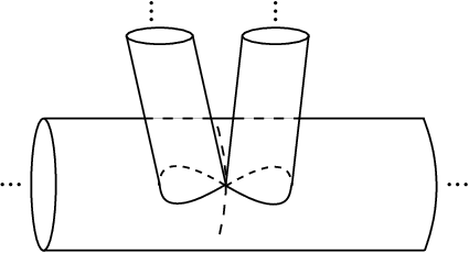
Refer to caption
Figure 4: wλw_{\lambda}

From Proposition 6.9 of [Bai], we have

Proposition 7.2.

The curve 𝒞λ\mathscr{C}_{\lambda} is a rational curve containing the points cλc_{\lambda}, cλ+1c_{\lambda+1}, wλw_{\lambda}, and pλp_{\lambda}. Every other point of 𝒞λ\mathscr{C}_{\lambda} represents a stable differential with two nonseparating nodes and two simple zeros.

We normalize every differential (X,ω)(X,\omega) in 𝒞λ\mathscr{C}_{\lambda} so that ω\omega has residues 11 and λ\lambda at two of the nodes.

Proposition 7.3.

With this normalization, the horizontal foliation of every (X,ω)∈𝒞λ(X,\omega)\in\mathscr{C}_{\lambda} is periodic.

Proof.

Each of the four half-infinite cylinders of (X,ω)(X,\omega) is bounded by a union of saddle connections. None of these saddle connections bounds two cylinders, or else (X,ω)(X,\omega) would be a one-point connected sum of two infinite cylinders and we would be done. Since ω\omega has two zeros, counting multiplicity, this means that every separatrix of (X,ω)(X,\omega) starts and ends at a zero. But this implies (X,ω)(X,\omega) is periodic. ∎

We now define a meromorphic quadratic differential qλq_{\lambda} on 𝒞λ\mathscr{C}_{\lambda} as we did on the leaves of 𝒜D\mathcal{A}_{D} in §4. Let 𝒞λ​(1,1)=𝒞λ∖{cλ,cλ+1,pλ,wλ}\mathscr{C}_{\lambda}(1,1)=\mathscr{C}_{\lambda}\setminus\{c_{\lambda},c_{\lambda+1},p_{\lambda},w_{\lambda}\}. Define a multivalued holomorphic function fλf_{\lambda} on 𝒞λ​(1,1)\mathscr{C}_{\lambda}(1,1) by

fλ​(X,ω)=∫pqω,f_{\lambda}(X,\omega)=\int_{p}^{q}\omega,

where pp and qq are the zeros of ω\omega, and define qλ=(∂fλ)2q_{\lambda}=(\partial f_{\lambda})^{2}.

Proposition 7.4.

The differential qλq_{\lambda} has double poles at cλc_{\lambda} and cλ+1c_{\lambda+1}, a simple pole at pλp_{\lambda}, a simple zero at wλw_{\lambda}, and is holomorphic and nonzero on 𝒞λ​(1,1)\mathscr{C}_{\lambda}(1,1). The horizontal foliation of qλq_{\lambda} is periodic, and the spine of qλq_{\lambda} coincides with the locus of two-cylinder surfaces.

Proof.

Any surface (X,ω)(X,\omega) sufficiently close to cλc_{\lambda} or cλ+1c_{\lambda+1} is a three cylinder surface with one finite area cylinder CC. Define a loop on 𝒞λ\mathscr{C}_{\lambda} by cutting (X,ω)(X,\omega) along a closed geodesic of CC and regluing after a rotation. This is a loop of length λ\lambda or λ+1\lambda+1 contained in the horizontal foliation of qλq_{\lambda}. Thus (𝒞λ,qλ)(\mathscr{C}_{\lambda},q_{\lambda}) has half-infinite cylinders around cλc_{\lambda} and cλ+1c_{\lambda+1}, so qλq_{\lambda} has double poles there.

The other zeros and poles are located just as for the quadratic differentials we defined along T​𝒜DT\mathcal{A}_{D} (see §10 of [Bai]).

Points along the separatrices emanating from pλp_{\lambda} and wλw_{\lambda} are obtained by performing a connected sum on pλp_{\lambda} or splitting the double zero of wλw_{\lambda} along a horizontal segment, which does not create a new cylinder. Thus the separatrices are contained in the two-cylinder locus, an embedded graph on 𝒞λ\mathscr{C}_{\lambda}. Thus the separatrices are saddle connections, and the horizontal foliation of qλq_{\lambda} is periodic.

By period coordinates, there is a tubular neighborhood UU of the spine such that ∂U\partial U consists of three cylinder surfaces. We then have at⋅∂U→{cλ∪cλ+1}a_{t}\cdot\partial U\to\{c_{\lambda}\cup c_{\lambda+1}\} as t→∞t\to\infty, so ∪at⋅U\cup a_{t}\cdot U covers 𝒞λ∖{cλ∪cλ+1}\mathscr{C}_{\lambda}\setminus\{c_{\lambda}\cup c_{\lambda+1}\}. It follows that the complement of the spine consists of three-cylinder surfaces as claimed. ∎

The surface (𝒞λ,qλ)(\mathscr{C}_{\lambda},q_{\lambda}) with its horizontal foliation is shown in Figure 5 with the spine indicated by a solid line. The singular points of the foliation with three or one prong are wλw_{\lambda} and pλp_{\lambda} respectively.

Figure 5: 𝒞λ\mathscr{C}_{\lambda} with the quadratic differential qλq_{\lambda}

The locus of three-cylinder surfaces in 𝒞λ\mathscr{C}_{\lambda} consists of two connected components. We refer to the component containing cλ+1c_{\lambda+1} as Uλ−U_{\lambda}^{-} and we call the other component Uλ+U_{\lambda}^{+}.

Curves in ∂XD\partial X_{D}.

In [Bai], we defined for every prototype P=(a,b,c,q¯)P=(a,b,c,\overline{q}) a curve CP⊂∂XDC_{P}\subset\partial X_{D} and a point cP∈∂XDc_{P}\in\partial X_{D}. The following properties of YDY_{D} are proved in §8 of that paper:

Theorem 7.5.

YDY_{D} has the following properties:

  • •

    ∂XD=⋃PCP\partial X_{D}=\bigcup_{P}C_{P}, where the union is over all prototypes of discriminant DD.

  • •

    CPC_{P} is a rational curve which intersects CP+C_{P^{+}} at cPc_{P} and intersects CP−C_{P^{-}} at cP−c_{P^{-}}. There are no other intersections between the curves CPC_{P}.

  • •

    The restriction of the natural morphism π:YD→ℙ​Ω​ℳ¯2\pi\colon Y_{D}\to{\mathbb{P}}\Omega\overline{\mathcal{M}}_{2} realizes CPC_{P} as a gcd⁡(a′,c′)\gcd(a^{\prime},c^{\prime})-fold branched cover of 𝒞λ⁡(P)\mathscr{C}_{\lambda(P)} with π⁡(cP)=cλ⁡(P)\pi(c_{P})=c_{\lambda(P)} and π⁡(cP−)=cλ⁡(P)+1\pi(c_{P^{-}})=c_{\lambda(P)+1}. The restriction π|CP\pi|_{C_{P}} is ramified to order gcd⁡(a′,c′)\gcd(a^{\prime},c^{\prime}) at these two points and is elsewhere unramified.

  • •

    The points cPc_{P} are cyclic quotient singularities of YDY_{D} of order

    mP=a′gcd⁡(a′,c′)​gcd⁡(a′,b′+c′),m_{P}=\frac{a^{\prime}}{\gcd(a^{\prime},c^{\prime})\gcd(a^{\prime},b^{\prime}+c^{\prime})}, (7.1)

    and are the only singular points in ∂XD\partial X_{D}.

  • •

    The curves P¯D\overline{P}_{D} and W¯D\overline{W}_{D} intersect CPC_{P} transversely in gcd⁡(a′,c′)\gcd(a^{\prime},c^{\prime}) points each and are disjoint from the points cQc_{Q}.

  • •

    The involution τ\tau of XDX_{D} extends to an involution τ\tau of YDY_{D} which sends CPC_{P} to Ct⁡(P)C_{t(P)}.

It follows from this theorem that ∂XD\partial X_{D} consists of finitely many chains of rational curves CPC_{P}. The connected components of ∂XD\partial X_{D} are naturally in bijection with the cusps of XDX_{D}.

We equip CPC_{P} with a quadratic differential qPq_{P} defined by,

qP=(π|CP)∗​qλ⁡(P).q_{P}=(\pi|_{C_{P}})^{*}q_{\lambda(P)}.

The locus of three-cylinder surfaces in CPC_{P} is the complement of the spine of qPq_{P} by Proposition 7.4. We define UP−⊂CPU_{P}^{-}\subset C_{P} to be the component of the three-cylinder locus containing cPc_{P}, and we define UP−+⊂CPU_{P^{-}}^{+}\subset C_{P} to be the component containing cP−c_{P^{-}}. Let SP⊂CPS_{P}\subset C_{P} be the spine of qPq_{P}, the two-cylinder locus.

Define

𝒰P=UP∪UP+∪UP−∪cP⊂YDσ,\mathcal{U}_{P}=U_{P}\cup U_{P}^{+}\cup U_{P}^{-}\cup c_{P}\subset Y_{D}^{\sigma},

where σ\sigma is the cusp of XDX_{D} corresponding to PP. The set 𝒰P\mathcal{U}_{P} is a neighborhood of cPc_{P}.

Local coverings.

Given a cusp σ\sigma of XDX_{D}, we defined the covering XDσ→XDX_{D}^{\sigma}\to X_{D} which is injective on a neighborhood 𝔑r\mathfrak{N}_{r} of the cusp of XDσX_{D}^{\sigma}. Let 𝔑¯r\overline{\mathfrak{N}}_{r} be the closure of 𝔑r\mathfrak{N}_{r} in YDY_{D}, and define YDσY_{D}^{\sigma} to be the complex orbifold obtained by gluing 𝔑¯r\overline{\mathfrak{N}}_{r} to XDσX_{D}^{\sigma}. Then YDσY_{D}^{\sigma} is a complex orbifold consisting of XDσX_{D}^{\sigma} together with a single chain of rational curves, and the natural map YDσ→YDY_{D}^{\sigma}\to Y_{D} is locally biholomorphic.

Each surface (X,[ω])∈YDσ(X,[\omega])\in Y_{D}^{\sigma} has a canonical horizontal direction, and we can normalize ω\omega (up to real multiple) so that the horizontal direction of ω\omega coincides with this canonical direction.

We then obtain an action of the upper-triangular subgroup B⊂SL2​ℝB\subset{\mathrm{SL}}_{2}{\mathbb{R}} on YDσY_{D}^{\sigma} coming from the action of GL2+​ℝ{\rm GL}_{2}^{+}{\mathbb{R}} on Ω​ℳ¯2\Omega{\overline{\mathcal{M}}}_{2}. This action fixes the points cPc_{P} and fixes SPS_{P} pointwise.

Type one coordinates.

We now describe local coordinates around points of CP∖{cP∪cP−}C_{P}\setminus\{c_{P}\cup c_{P^{-}}\} which will be used in the proof of Lemma 8.3.

Let W⊂𝒞λ∖{cλ,cλ+1}W\subset\mathscr{C}_{\lambda}\setminus\{c_{\lambda},c_{\lambda+1}\} be a simply connected domain. For each z∈Wz\in W, write (Xz,ωz)(X_{z},\omega_{z}) for the associated stable differential, normalized as before so that the residues at the nonseparating nodes are 11 and λ\lambda. Write N={n1,n2}⊂XzN=\{n_{1},n_{2}\}\subset X_{z} for the set of nonseparating nodes with n1n_{1} being the residue 11 node. Choose homology classes

αi∈H1​(Xz∖Nz,ℤ)andβi∈H1​(Xz,Nz,ℤ)\alpha_{i}\in H_{1}(X_{z}\setminus N_{z};{\mathbb{Z}})\quad\text{and}\quad\beta_{i}\in H_{1}(X_{z},N_{z};{\mathbb{Z}})

so that αi\alpha_{i} goes around nin_{i}, and αi⋅βj=δi​j\alpha_{i}\cdot\beta_{j}=\delta_{ij}. Choose these classes consistently so that they are parallel with respect to the Gauss-Manin connection.

We can plumb the nodes nin_{i} as described in §3 to obtain a new surface (Xz′,ωz′)(X_{z}^{\prime},\omega_{z}^{\prime}). The homology class βi\beta_{i} becomes a class in H1​(Xz′,ℤ)H_{1}(X_{z}^{\prime};{\mathbb{Z}}) which we will continue to call βi\beta_{i}. It is well defined up to adding a multiple of αi\alpha_{i}. If wiw_{i} is sufficiently large, then there is a unique way to plumb the node nin_{i} so that

e2​π​i​ωz′​(βi)/ωz′​(αi)=wi.e^{2\pi i\omega^{\prime}_{z}(\beta_{i})/\omega^{\prime}_{z}(\alpha_{i})}=w_{i}. (7.2)

Let Plumb⁡(z,w1,w2)\Plumb(z,w_{1},w_{2}) be the result of plumbing (Xz,ωz)(X_{z},\omega_{z}) so that (7.2) holds. If one of the wiw_{i} is zero, the corresponding node of (Xz,ωz)(X_{z},\omega_{z}) remains a node of Plumb⁡(z,w1,w2)\Plumb(z,w_{1},w_{2}).

Let U⊂CPU\subset C_{P} be a component of π−1​(W)\pi^{-1}(W). Define f:U×V→YDσf\colon U\times V\to Y_{D}^{\sigma} by

f(u,v)=Plumb(π(u),v−c′/gcd(a′,c′),rva′/gcd⁡(a′,c′)),f(u,v)=\Plumb(\pi(u),v^{-c^{\prime}/\gcd(a^{\prime},c^{\prime})},rv^{a^{\prime}/\gcd(a^{\prime},c^{\prime})}),

where rr satisfies

r−c′=e2​π​i​q′,r^{-c^{\prime}}=e^{2\pi iq^{\prime}}, (7.3)

and V⊂ℂV\subset{\mathbb{C}} is a neighborhood of 00 small enough that ff is defined on U×VU\times V.

From Theorem 7.22 and Proposition 8.1 of [Bai], we have:

Theorem 7.6.

For some choice of rr satisfying (7.3), ff is biholomorphic onto its image in YDσY_{D}^{\sigma}, a neighborhood of U⊂CPU\subset C_{P}.

Remark.

The choice of rr in (7.3) is equivalent to the choice of the component UU of π−1​(W)\pi^{-1}(W).

It follows that ff defines coordinates (u,v)(u,v) around points in UU. We will call these type one coordinates.

Type two coordinates.

We now describe local coordinates around the points cP∈YDc_{P}\in Y_{D}. Define Rλ:Δ3→ℙ​Ω​ℳ¯2R_{\lambda}\colon\Delta^{3}\to{\mathbb{P}}\Omega\overline{\mathcal{M}}_{2} by

Rλ​(w1,w2,w3)=S⁡(1,λ,λ−1,12​π​i​log⁡w1,λ2​π​i​log⁡w2,λ−12​π​i​log⁡w3),R_{\lambda}(w_{1},w_{2},w_{3})=S\left(1,\lambda,\lambda-1,\frac{1}{2\pi i}\log w_{1},\frac{\lambda}{2\pi i}\log w_{2},\frac{\lambda-1}{2\pi i}\log w_{3}\right),

where if wi=0w_{i}=0, then the corresponding cylinder is instead a node. Define gP:Δ2→ℙ​Ω​ℳ¯2g_{P}\colon\Delta^{2}\to{\mathbb{P}}\Omega\overline{\mathcal{M}}_{2} by

gP(u,v)=Rλ⁡(P)(e2​π​i​q′/a′u−c′/gcd(a′,c′)v−(a′+b′+c′)/gcd(a′,a′+b′+c′),OPENua′/gcd⁡(a′,c′),va′/gcd⁡(a′,a′+b′+c′)).g_{P}(u,v)=R_{\lambda(P)}\bigg(e^{2\pi iq^{\prime}/a^{\prime}}u^{-c^{\prime}/\gcd(a^{\prime},c^{\prime})}v^{-(a^{\prime}+b^{\prime}+c^{\prime})/\gcd(a^{\prime},a^{\prime}+b^{\prime}+c^{\prime})},\\ u^{a^{\prime}/\gcd(a^{\prime},c^{\prime})},v^{a^{\prime}/\gcd(a^{\prime},a^{\prime}+b^{\prime}+c^{\prime})}\bigg).

Given relatively prime m,s∈ℤm,s\in{\mathbb{Z}} with m>0m>0, let θm\theta_{m} be an mm-th root of unity, and let Γm,s\Gamma_{m,s} be the group of automorphisms of Δ2\Delta^{2} generated by

(z,w)↦(θm​z,θms​w).(z,w)\mapsto(\theta_{m}z,\theta_{m}^{s}w).

From Theorem 7.27 and Proposition 8.3 of [Bai], we have

Theorem 7.7.

gPg_{P} lifts to a holomorphic map f:Δ2→YDσf\colon\Delta^{2}\to Y_{D}^{\sigma}, and ff descends to a map f~:Δ2/Γm,s→YDσ\widetilde{f}\colon\Delta^{2}/\Gamma_{m,s}\to Y_{D}^{\sigma}, where m=mPm=m_{P} defined in (7.1). The map ff is biholomorphic onto its image 𝒰P\mathcal{U}_{P}, a neighborhood of cPc_{P}. Furthermore,

f−1​(CP)\displaystyle f^{-1}(C_{P}) ={(u,v)∈Δ2:u=0}\displaystyle=\{(u,v)\in\Delta^{2}\colon u=0\}
f−1​(CP+)\displaystyle f^{-1}(C_{P^{+}}) ={(u,v)∈Δ2:v=0}.\displaystyle=\{(u,v)\in\Delta^{2}\colon v=0\}.

We call the coordinates (u,v)(u,v) induced by ff on the neighborhood 𝒰P\mathcal{U}_{P} of cPc_{P} type two coordinates.

Singularities of ℱD\mathcal{F}_{D}.

We finish this section by discussing the geometry of the foliation ℱD\mathcal{F}_{D} near ∂XD\partial X_{D}.

Proposition 7.8.

The foliation ℱD\mathcal{F}_{D} extends to a foliation of

YD∖⋃P∈𝒴D(cP∪SP)Y_{D}\setminus\bigcup_{P\in\mathcal{Y}_{D}}(c_{P}\cup S_{P}) (7.4)

and does not extend to any larger set.

Proof.

We work in a local covering YDσY_{D}^{\sigma} where the leaves of ℱD\mathcal{F}_{D} are the orbits of BB. Since the BB-action is free on the locus (7.4), its orbits there are the required extension of ℱD\mathcal{F}_{D}.

In the neighborhood 𝒰P\mathcal{U}_{P} of cPc_{P}, the horizontal foliation of every surface (X,ω)(X,\omega) has three cylinders, so at⋅(X,ω)→cPa_{t}\cdot(X,\omega)\to c_{P}. Thus every leaf of ℱD\mathcal{F}_{D} near cPc_{P} passes through cPc_{P}, which is impossible if ℱD\mathcal{F}_{D} can be extended to a foliation.

Suppose ℱD\mathcal{F}_{D} can be extended over a neighborhood of p∈SPp\in S_{P}. Choose type one coordinates (u,v)(u,v) around pp so that p=(0,0)p=(0,0). In these coordinates {0}×Δϵ\{0\}\times\Delta_{\epsilon} is contained in a leaf of ℱD\mathcal{F}_{D} transverse to CPC_{P}. The subsets UP−U_{P}^{-} and UP−+U_{P^{-}}^{+} of CPC_{P} are also contained in leaves of ℱD\mathcal{F}_{D}. Thus CPC_{P} is a leaf of ℱD\mathcal{F}_{D} near pp, a contradiction because then ℱD\mathcal{F}_{D} would have two leaves meeting at pp. ∎

8 ℱD\mathcal{F}_{D} as a current on YDY_{D}

We saw in Proposition 7.8 that ℱD\mathcal{F}_{D} doesn’t extend to a foliation of YDY_{D}. Nevertheless, we will show in this section that the closed current on XDX_{D} defined by the measured foliation ℱD\mathcal{F}_{D} does extend to YDY_{D}:

Theorem 8.1.

Integration of smooth 22-forms on YDY_{D} over ℱD\mathcal{F}_{D} defines a closed 22-current on YDY_{D}.

We will then use this to interpret vol⁡ED​(1,1)\vol E_{D}(1,1) as an intersection of classes in H2​(YD,ℝ)H^{2}(Y_{D};{\mathbb{R}}).

Poincaré growth.

Let X¯\overline{X} be a compact, complex orbifold, and let X⊂X¯X\subset\overline{X} be the complement of a divisor DD. Suppose DD is covered by coordinate charts of the form Δn/G\Delta^{n}/G, where

  • •

    Each transformation g∈Gg\in G is of the form,

    g⁡(z1,…,zn)=(θ1​z1,…,θn​zn),g(z_{1},\ldots,z_{n})=(\theta_{1}z_{1},\ldots,\theta_{n}z_{n}),

    for some roots of unity θi\theta_{i};

  • •

    D∩ΔD\cap\Delta is a union of the coordinate axes z1=0,…,zr=0z_{1}=0,\ldots,z_{r}=0 for 1≤r≤n1\leq r\leq n.

In such a chart Δn/G\Delta^{n}/G, we have Δn∩X=(Δ∗)r×Δn−r\Delta^{n}\cap X=(\Delta^{*})^{r}\times\Delta^{n-r}. We give Δn∩X\Delta^{n}\cap X a metric ρ\rho by putting the Poincaré metric,

d​s2=|d​z|2|z|2​(log⁡|z|)2,ds^{2}=\frac{|dz|^{2}}{|z|^{2}(\log|z|)^{2}},

on the Δ∗\Delta^{*} factors, putting the Euclidean metric |d​z|2|dz|^{2} on the Δ\Delta factors, and defining ρ\rho to be the product metric. Following Mumford [Mum77], we say that a form ω\omega on XX has Poincaré growth if there is a covering of DD by charts Uα/GαU_{\alpha}/G_{\alpha} with metrics ρα\rho_{\alpha} of this form such that for each α\alpha,

‖ω‖ρα≺1.\|\omega\|_{\rho_{\alpha}}\prec 1.

Let ωi\omega_{i} be the 22-form on XDX_{D} covered by the forms,

ω~i=12​π​d​xi∧d​yiyi2,\widetilde{\omega}_{i}=\frac{1}{2\pi}\frac{dx_{i}\wedge dy_{i}}{y_{i}^{2}},

on ℍ×ℍ{\mathbb{H}}\times{\mathbb{H}}.

Proposition 8.2.

The forms ωi\omega_{i} have Poincaré growth. Furthermore, there are smooth 11-forms ηi\eta_{i} on XDX_{D} with Poincaré growth such that ωi−d​ηi\omega_{i}-d\eta_{i} are smooth 22-forms on YDY_{D}. Integration against ωi\omega_{i} defines a closed 22-current on YDY_{D}.

Proof.

We showed in [Bai, Proposition 2.8] that ωi\omega_{i} is the Chern form of a metric hih_{i} on a line bundle Qi​YDQ^{i}Y_{D} over YDY_{D}, and we showed in [Bai, Theorem 9.8] that hih_{i} is what Mumford calls a good metric in [Mum77]. It follows from [Mum77, Theorem 1.4] that the ωi\omega_{i} have Poincaré growth. The second statement follows from the proof of the same theorem, and the last statement follows from Propositions 1.1 and 1.2 of [Mum77]. ∎

Bounded norm.

In order to prove Theorem 8.1, we need to bound the norm ‖ω‖ℱD\|\omega\|_{\mathcal{F}_{D}} for smooth forms ω\omega on YDY_{D}. In fact, we will need these bounds for forms which just have Poincaré growth.

Lemma 8.3.

For any pp-form ω\omega on XDX_{D} with Poincaré growth, ‖ω‖ℱD\|\omega\|_{\mathcal{F}_{D}} is bounded.

Proof.

Let U⊂YDU\subset Y_{D} be an open set meeting ∂XD\partial X_{D} with the coordinates (u,v)(u,v) defined in §7. Let K⊂UK\subset U be compact. Let ρ\rho be the metric on UU as defined above. Since ‖ω‖ρ\|\omega\|_{\rho} is bounded on KK, it suffices to show that ‖v‖ρ/‖v‖ℱD\|v\|_{\rho}/\|v\|_{\mathcal{F}_{D}} is bounded on KK for any vector field vv tangent to ℱD\mathcal{F}_{D} (where ‖v‖ℱD\|v\|_{\mathcal{F}_{D}} denotes the norm of vv with respect to the hyperbolic metric on leaves of ℱD\mathcal{F}_{D}). Since ℱD\mathcal{F}_{D} is one-dimensional, it suffices to show ‖v‖ρ\|v\|_{\rho} is bounded for a single vector field vv tangent to ℱD\mathcal{F}_{D} with unit ℱD\mathcal{F}_{D}-norm. There are two cases, depending on whether or not UU is a type one or type two coordinate chart.

First suppose UU is a type two coordinate chart around cPc_{P} in YDY_{D}. If UU is small enough, we can regard it as a subset of UPU_{P} from §6. By Theorem 6.4, the universal cover U~P\widetilde{U}_{P} is isomorphic to ℍ×ℍ{\mathbb{H}}\times{\mathbb{H}} with coordinates (y2,y3)(y_{2},y_{3}) from §6. The (u,v)(u,v)-coordinates are related to the (y2,y3)(y_{2},y_{3})-coordinates by

u=ei​c2​y2andv=ei​c3​y3,u=e^{ic_{2}y_{2}}\quad\text{and}\quad v=e^{ic_{3}y_{3}},

for positive real constants c2c_{2} and c3c_{3}. The action of the diagonal group A⊂SL2​ℝA\subset{\mathrm{SL}}_{2}{\mathbb{R}} on U~P\widetilde{U}_{P} is given by

at⋅(u2+i​v2,u3+i​v3)=(u2+i​et​v2,u3+i​et​v3),a_{t}\cdot(u_{2}+iv_{2},u_{3}+iv_{3})=(u_{2}+ie^{t}v_{2},u_{3}+ie^{t}v_{3}),

where yj=uj+i​vjy_{j}=u_{j}+iv_{j}. Thus

v=Im⁡y2​∂∂y2+Im⁡y3​∂∂y3v=\IM y_{2}\frac{\partial}{\partial y_{2}}+\IM y_{3}\frac{\partial}{\partial y_{3}}

is a unit length tangent vector field to the lift of ℱD\mathcal{F}_{D} to U~P\widetilde{U}_{P}. In the (u,v)(u,v)-coordinates,

v=−i​u​log⁡|u|​∂∂u−i​v​log⁡|v|​∂∂v.v=-iu\log|u|\frac{\partial}{\partial u}-iv\log|v|\frac{\partial}{\partial v}.

This is a unit length vector field tangent to ℱD\mathcal{F}_{D} with bounded ρ\rho-length.

The case when UU is a type one coordinate chart is similar. For some function ff, the vector field,

v=f⁡(u,v)​∂∂u−i​v​log⁡|v|​∂∂v,v=f(u,v)\frac{\partial}{\partial u}-iv\log|v|\frac{\partial}{\partial v},

is a unit length vector field tangent to ℱD\mathcal{F}_{D}. The function ff is continuous because vv is tangent to the flow on YDY_{D} generated by AA. Therefore ‖v‖ρ\|v\|_{\rho} is bounded on KK. ∎

Corollary 8.4.

For any 2-form ω\omega on XX with Poincaré growth,

∫ℱD|ω|<∞.\int_{\mathcal{F}_{D}}|\omega|<\infty. (8.1)

In particular, ℱD\mathcal{F}_{D} defines a current on YDY_{D}.

Proof.

The first statement follows directly from Lemma 8.3 since μD\mu_{D} has finite volume by Theorem 4.6. Since any smooth form on YDY_{D} has Poincaré growth, (8.1) holds in particular for smooth forms. For ℱD\mathcal{F}_{D} to define a current, it suffices to show that if ωn→0\omega_{n}\to 0 is a uniformly convergent sequence of forms on YDY_{D}, then ∫ℱDωn→0\int_{\mathcal{F}_{D}}\omega_{n}\to 0. This is easily seen from the proof of Lemma 8.3 using the fact that ‖ωn‖ρ→0\|\omega_{n}\|_{\rho}\to 0 in each chart UU. ∎

Cusp neighborhoods.

The proof that ℱD\mathcal{F}_{D} is closed, will require certain well-behaved neighborhoods of the cusps of XDX_{D}.

Lemma 8.5.

For any ϵ>0\epsilon>0, there is a closed, HH-invariant neighborhood W⊂XDW\subset X_{D} of the cusps of XDX_{D} such that vol⁡W<ϵ\Vol W<\epsilon and ∂W\partial W is a submanifold of XDX_{D} transverse to ℱD\mathcal{F}_{D}.

Proof.

It suffices to construct a neighborhood of the cusp at infinity in the covering XDσX_{D}^{\sigma} with the required properties. Let ρ:ℝ→ℝ\rho\colon{\mathbb{R}}\to{\mathbb{R}} be smooth and increasing with ρ⁡(x)=0\rho(x)=0 for x<1/2x<1/2 and ρ⁡(x)=x\rho(x)=x for x>1x>1. Recall that each point in XDσX_{D}^{\sigma} represents an eigenform (X,ω)(X,\omega) together with a choice of horizontal direction. Normalize each (X,ω)(X,\omega) to have unit area. Define a smooth function ff on XDσX_{D}^{\sigma} by

f⁡(X,ω)=∑iρ⁡(height⁡(Ci)),f(X,\omega)=\sum_{i}\rho(\height(C_{i})),

where the sum is over the horizontal cylinders of XDX_{D} (ff is zero if there are no horizontal cylinders). The bump function ρ\rho is there to make ff smooth; otherwise ff would just be continuous.

Let Wℓ=f−1[ℓ,∞)W_{\ell}=f^{-1}[\ell,\infty). The function ff is HH-invariant, so WℓW_{\ell} is as well. We have f⁡(x)→∞f(x)\to\infty as xx approaches the cusp of XDσX_{D}^{\sigma} because surfaces develop tall cylinders as they approach the cusp (see Theorem 5.5 and Proposition 7.1 of [Bai]). Thus WℓW_{\ell} is a neighborhood of the cusp.

If f⁡(X,ω)>0f(X,\omega)>0, then dd​t​f​(at⋅(X,ω))>0\frac{d}{dt}f(a_{t}\cdot(X,\omega))>0. It follows that ℓ\ell is a regular value of ff, so ∂Wℓ\partial W_{\ell} is smooth if ℓ>0\ell>0. Also if ℓ>0\ell>0, then ∂Wℓ\partial W_{\ell} is transverse to ℱD\mathcal{F}_{D}.

Since XDX_{D} has finite volume, the cusp of XDσX_{D}^{\sigma} does as well, so vol⁡Wℓ→0\Vol W_{\ell}\to 0 as ℓ→∞\ell\to\infty. ∎

Given WW as in Lemma 8.5, let 𝒲\mathcal{W} be the measured foliation of ∂W\partial W induced by ℱD\mathcal{F}_{D}. Give the leaves of 𝒲\mathcal{W} their arclength measure as horocycles in ℍ{\mathbb{H}}, and let ν\nu be the measure on ∂W\partial W which is the product of the leafwise and transverse measures.

Lemma 8.6.

We have

vol∂W=volW\vol\partial W=\vol W

with respect to the measures ν\nu and μD\mu_{D}.

Proof.

This follows directly from the fact that the length of the horocycle in ℍ{\mathbb{H}} joining ii to i+ti+t is equal to the area of the region in ℍ{\mathbb{H}} lying above this horocycle. ∎

Proof of Theorem 8.1.

After Corollary 8.4, it remains to show that the current defined by integration over ℱD\mathcal{F}_{D} is closed. Let η\eta be a smooth 11-form on YDY_{D}. We need to show ∫ℱD𝑑η=0\int_{\mathcal{F}_{D}}d\eta=0.

Since η\eta is smooth, η\eta and d​ηd\eta have Poincaré growth, so ‖η‖ℱD\|\eta\|_{\mathcal{F}_{D}} and ‖η‖ℱD\|\eta\|_{\mathcal{F}_{D}} are bounded. Given ϵ>0\epsilon>0, let W⊂XDW\subset X_{D} be the neighborhood of the cusps constructed in Lemma 8.5 with vol⁡W<ϵ\Vol W<\epsilon. By Stokes’ Theorem and Lemma 8.6,

∫ℱD𝑑η\displaystyle\int_{\mathcal{F}_{D}}d\eta =∫ℱD|W𝑑η+∫𝒲η\displaystyle=\int_{\mathcal{F}_{D}|_{W}}d\eta+\int_{\mathcal{W}}\eta
≤ϵ⁡(‖η‖ℱD∞+‖d​η‖ℱD∞)\displaystyle\leq\epsilon(\|\eta\|_{\mathcal{F}_{D}}^{\infty}+\|d\eta\|_{\mathcal{F}_{D}}^{\infty})

where the last integral is over the measured foliation of 𝒲\mathcal{W} of ∂W\partial W defined above. Thus ∫ℱD𝑑η=0\int_{\mathcal{F}_{D}}d\eta=0. ∎

Cohomological interpretation of vol⁡ED​(1,1)\vol E_{D}(1,1).

Let [ℱ¯D],[ωi]∈H2​(YD,ℝ)[\overline{\mathcal{F}}_{D}],[\omega_{i}]\in H^{2}(Y_{D};{\mathbb{R}}) be the cohomology classes defined by the respective closed currents.

Theorem 8.7.

We have

vol⁡ED​(1,1)=2​π​[ω1]⋅[ℱ¯D],\vol E_{D}(1,1)=2\pi[\omega_{1}]\cdot[\overline{\mathcal{F}}_{D}],

where the pairing is the intersection pairing on H2​(YD,ℝ)H^{2}(Y_{D};{\mathbb{R}}).

Proof.

By Proposition 8.2, there is a smooth 11-form η\eta on XDX_{D} with Poincaré growth such that

α=ω1−d​η\alpha=\omega_{1}-d\eta

is a smooth 22-form on YDY_{D}. We have,

[ω1]⋅[ℱ¯D]\displaystyle[\omega_{1}]\cdot[\overline{\mathcal{F}}_{D}] =∫ℱDα\displaystyle=\int_{\mathcal{F}_{D}}\alpha
=∫ℱDω1−∫ℱD𝑑η\displaystyle=\int_{\mathcal{F}_{D}}\omega_{1}-\int_{\mathcal{F}_{D}}d\eta
=∫ℱDω1\displaystyle=\int_{\mathcal{F}_{D}}\omega_{1}
=12​π​vol⁡ED​(1,1).\displaystyle=\frac{1}{2\pi}\vol E_{D}(1,1).

∎

9 Intersection with closed leaves

In this section, we will relate the foliation ℱD\mathcal{F}_{D} in a neighborhood of PDP_{D} and WDW_{D} with the canonical foliations of the tangent bundles of these curves. This, together with Theorem 2.3 will imply that the classes [P¯D][\overline{P}_{D}] and [W¯D][\overline{W}_{D}] have trivial intersection with [ℱ¯D][\overline{\mathcal{F}}_{D}].

Bundles over YDY_{D}.

The line bundle Ω​XD\Omega X_{D} over XDX_{D} defined in §4 extends to a line bundle Ω​YD\Omega Y_{D} over YDY_{D} whose fiber over (X,[ω])(X,[\omega]) is the line in Ω⁡(X)\Omega(X) determined by [ω][\omega]. Let Q​YD=(Ω​YD)2QY_{D}=(\Omega Y_{D})^{2}, the line bundle whose fiber over (X,[ω])(X,[\omega]) is the space Q​XQX of quadratic differentials on XX which are multiples of ω2\omega^{2}. The L1L^{1}-metric on Q​YDQY_{D} is the Hermitian metric which assigns to qq norm ∫X|q|\int_{X}|q|.

Cotangent bundles.

For the rest of this section, CC will denote either of the curves PDP_{D} or WDW_{D}. For any curve E⊂YDE\subset Y_{D}, we let Q​EQE denote the restriction of Q​YDQY_{D} to EE. We start by sketching a proof of the following well-known fact from Teichmüller theory:

Proposition 9.1.

There is a natural isomorphism,

Q​C→T∗​C,QC\to T^{*}C, (9.1)

which identifies the L1L^{1}-metric on Q​CQC with twice the hyperbolic metric on T∗​CT^{*}C.

Proof.

Suppose C=WDC=W_{D}. Given (X,[ω])∈WD(X,[\omega])\in W_{D}, the quadratic differential ω2\omega^{2} defines via Teichmüller theory a cotangent vector τ\tau to ℳ2{\mathcal{M}}_{2} at XX. Pulling back τ\tau by the immersion WD→ℳ2W_{D}\to{\mathcal{M}}_{2} defines a cotangent vector σ\sigma to WDW_{D} at (X,[ω])(X,[\omega]). This defines the map (9.1).

Consider the unit speed geodesic (Xt,ωt)=at⋅(X,ω)(X_{t},\omega_{t})=a_{t}\cdot(X,\omega) on WDW_{D}. The induced Teichmüller map ft:X→Xtf_{t}\colon X\to X_{t} has complex dilatation,

μt=e−t/2−et/2e−t/2+et/2​ν,\mu_{t}=\frac{e^{-t/2}-e^{t/2}}{e^{-t/2}+e^{t/2}}\nu,

where ν=ω¯/ω\nu=\overline{\omega}/\omega. We have

dd​t​μt=−12​ν,\frac{d}{dt}\mu_{t}=-\frac{1}{2}\nu,

so ν\nu represents a tangent vector to WDW_{D} of hyperbolic norm 22. The pairing with σ\sigma is given by

⟨σ,ν⟩=∫ω¯ω​ω2=∫|ω2|=‖ω2‖,\langle\sigma,\nu\rangle=\int\frac{\overline{\omega}}{\omega}\omega^{2}=\int|\omega^{2}|=\|\omega^{2}\|,

so the hyperbolic norm of σ\sigma is half the L1L^{1} norm.

The case where C=PDC=P_{D} is identical, except that we use the immersion PD→ℳ1×ℳ1P_{D}\to{\mathcal{M}}_{1}\times{\mathcal{M}}_{1} instead of ℳ2{\mathcal{M}}_{2}. ∎

Lemma 9.2.

The natural isomorphism (9.1) extends to an isomorphism,

Q​C¯→T∗​C¯​(D),Q\overline{C}\to T^{*}\overline{C}(D),

where the divisor DD is the sum of the cusps of CC.

Proof.

Given a cusp cc, we need to construct a nonzero holomorphic section of Q​C¯Q\overline{C} on a neighborhood of cc whose associated section of T∗​C¯T^{*}\overline{C} has a simple pole at cc. Let (X,ω)∈C(X,\omega)\in C with at⋅(X,ω)→ca_{t}\cdot(X,\omega)\to c at t→∞t\to\infty. Let hrh_{r} be a generator of the subgroup of the stabilizer Stab⁡(X,ω)⊂SL2​ℝ\Stab(X,\omega)\subset{\mathrm{SL}}_{2}{\mathbb{R}} which stabilizes (X,ω)(X,\omega). Define a holomorphic map f:Δ→Cf\colon\Delta\to C by f⁡(w)=(Xw,ωw)f(w)=(X_{w},\omega_{w}), where if w≠0w\neq 0, then

(Xw,ωw)=(1r2​π​arg⁡w0r2​π​log⁡1|w|)⋅(X,ω),(X_{w},\omega_{w})=\begin{pmatrix}1&\dfrac{r}{2\pi}\arg w\\ 0&\dfrac{r}{2\pi}\log\dfrac{1}{|w|}\end{pmatrix}\cdot(X,\omega),

and (X0,ω0)(X_{0},\omega_{0}) is the unique limiting stable Abelian differential, which is visibly nonzero. The restriction of ff to some Δϵ\Delta_{\epsilon} is a conformal isomorphism onto some neighborhood of cc.

We have a nonzero holomorphic section w↦ωw2w\mapsto\omega_{w}^{2} of Q​C¯Q\overline{C} over Δϵ\Delta_{\epsilon}. The associated holomorphic 11-form τ\tau on Δϵ∗\Delta^{*}_{\epsilon} has hyperbolic norm,

‖τ‖=12​∫X|ωw|2≍−log⁡|w|,\|\tau\|=\frac{1}{2}\int_{X}|\omega_{w}|^{2}\asymp-\log|w|,

with respect to the hyperbolic metric on Δϵ∗\Delta^{*}_{\epsilon}. Since a nonzero holomorphic section of T∗​ΔϵT^{*}\Delta_{\epsilon} has norm comparable to −|w|​log⁡|w|-|w|\log|w|, τ\tau has a simple pole at 00. ∎

Foliated tubular neighborhoods.

Let U⊂ℙ​Ω​ℳ¯2U\subset{\mathbb{P}}\Omega\overline{\mathcal{M}}_{2} be a tubular neighborhood of C¯\overline{C} which is small enough that each point of U∖C¯U\setminus\overline{C} represents a surface with a unique shortest saddle connection (up to the hyperelliptic involution) connecting distinct zeros.

Define a map Φ:U→(Q​C¯)∗\Phi\colon U\to(Q\overline{C})^{*} as follows. Given (X,ω)∈U(X,\omega)\in U, let I⊂XI\subset X be the unique shortest saddle connection connecting distinct zeros, and let (Y,η)(Y,\eta) be the surface obtained by collapsing II. Identify Q​YQY with Q​XQX by the unique linear map TT sending η2\eta^{2} to ω2\omega^{2}. Define S∈(Q​YD)∗S\in(QY_{D})^{*} by

S⁡(q)=(∫IT⁡(q))2,S(q)=\left(\int_{I}\sqrt{T(q)}\right)^{2},

and define Φ⁡(X,ω)=(Y,S)\Phi(X,\omega)=(Y,S).

We observed in the proof of [Bai, Theorem 12.2]:

Proposition 9.3.

In the case where C=PDC=P_{D}, the map Φ\Phi is an isomorphism between UU and a neighborhood of the zero section in (Q​P¯D)∗(Q\overline{P}_{D})^{*}. In the case where C=WDC=W_{D}, there is a tubular neighborhood V⊂UV\subset U which is a threefold branched covering by Φ\Phi of a neighborhood of the zero section in (Q​W¯D)∗(Q\overline{W}_{D})^{*}, branched over W¯D\overline{W}_{D}.

The proof is essentially immediate from the fact that given a short segment I⊂ℂI\subset{\mathbb{C}}, there are three ways to split a double zero along II and one way to perform a connected sum along II.

Proposition 9.4.

The map Φ\Phi sends the foliation ℱD\mathcal{F}_{D} to 2​i2i times the canonical foliation of T​CTC.

Proof.

Given (X,ω)∈C(X,\omega)\in C, identify the universal cover C~\widetilde{C} with ℍ{\mathbb{H}} by z↦(Xz,ωz)z\mapsto(X_{z},\omega_{z}), where

(Xz,ωz)=(1Re⁡z0Im⁡z)⋅(X,ω).(X_{z},\omega_{z})=\begin{pmatrix}1&\RE z\\ 0&\IM z\end{pmatrix}\cdot(X,\omega).

By the proof of Proposition 9.1, the Beltrami differential νz=ω¯z/ωz\nu_{z}=\overline{\omega}_{z}/\omega_{z} on XzX_{z} represents the tangent at zz to the geodesic γ⁡(s)=es​z\gamma(s)=e^{s}z at s=ts=t, that is, the vector

vz=−2​i​y​∂∂z,v_{z}=-2iy\frac{\partial}{\partial z},

at zz.

Now restrict to the case where C=PDC=P_{D}. Let U⊂ℍU\subset{\mathbb{H}} be a small neighborhood of ii. Given w∈ℂ∖{0}w\in{\mathbb{C}}\setminus\{0\} let Iw∈ℂI_{w}\in{\mathbb{C}} be the segment joining w/2\sqrt{w}/2 and −w/2-\sqrt{w}/2. Choose some ϵ\epsilon small enough that for every w∈Δϵw\in\Delta_{\epsilon} and z∈Uz\in U, we can form the connected sum of (Xz,ωz)(X_{z},\omega_{z}) along IwI_{w}. We parameterize a neighborhood of (X,ω)(X,\omega) in YDY_{D} by f:U×Δϵ→YDf\colon U\times\Delta_{\epsilon}\to Y_{D}, where

f⁡(z,w)=Sum⁡((Xz,ωz),Iw).f(z,w)=\connsum((X_{z},\omega_{z}),I_{w}). (9.2)

In these (z,w)(z,w)-coordinates, we have Φ⁡(z,w)=(Xz,Sw),\Phi(z,w)=(X_{z},S_{w}), where Sw∈(Q​X)∗S_{w}\in(QX)^{*} is characterized by S⁡(ωz2)=w,S(\omega_{z}^{2})=w, which corresponds to the Beltrami differential,

wIm⁡z​νz,\frac{w}{\IM z}\nu_{z},

which in turn corresponds to the tangent vector,

−2​i​w​∂∂z.-2iw\frac{\partial}{\partial z}.

Thus, identifying (Q​PD)∗(QP_{D})^{*} with T​PDTP_{D}, we have

i2​Φ​(z,w)=(z,w​∂∂z).\frac{i}{2}\Phi(z,w)=\left(z,w\frac{\partial}{\partial z}\right). (9.3)

We have,

(1Re⁡z0Im⁡z)⋅Sum⁡((X,ω),I(u+i​v)2)=Sum⁡((Xz,ωz),I(u+z​v)2),\begin{pmatrix}1&\RE z\\ 0&\IM z\end{pmatrix}\cdot\connsum((X,\omega),I_{(u+iv)^{2}})=\connsum((X_{z},\omega_{z}),I_{(u+zv)^{2}}),

so in (z,w)(z,w) coordinates, the leaf of ℱD\mathcal{F}_{D} through (i,(u+i​v)2)(i,(u+iv)^{2}) is parameterized by z↦(z,(u+z​v)2)z\mapsto(z,(u+zv)^{2}), which corresponds to the leaf of 𝒞PD\mathcal{C}_{P_{D}} through i2​Φ​(i,w)\frac{i}{2}\Phi(i,w).

The proof in the case where C=WDC=W_{D} is nearly identical except that we use the operation of splitting a double zero to parameterize a tubular neighborhood of WDW_{D}. Recall that a splitting of a double zero of a differential (X,ω)(X,\omega) is determined by an embedded “X” as defined in §3. Equation (9.2) becomes

f⁡(z,w)=Split⁡((Xz,ωz),Ez​(w)),f(z,w)=\zerosplit((X_{z},\omega_{z}),E_{z}(w)),

where EzE_{z} is a holomorphic map from some small disk Δϵ⊂ℂ\Delta_{\epsilon}\subset{\mathbb{C}} to the space of embedded “X”s on (Xz,ωz)(X_{z},\omega_{z}) such that for each segment II of Ez​(w)E_{z}(w),

(∫Iωz)2=w3.\left(\int_{I}\omega_{z}\right)^{2}=w^{3}.

Then, (9.3) becomes

i2​Φ​(z,w)=(z,w3​∂∂z).\frac{i}{2}\Phi(z,w)=\left(z,w^{3}\frac{\partial}{\partial z}\right).

∎

Theorem 9.5.

We have,

[PD]⋅[ℱ¯D]=[WD]⋅[ℱ¯D]=0.[P_{D}]\cdot[\overline{\mathcal{F}}_{D}]=[W_{D}]\cdot[\overline{\mathcal{F}}_{D}]=0. (9.4)
Proof.

Let Ψ\Psi be the form defined in §2 which represents the Thom class on T​P¯D​(−D)T\overline{P}_{D}(-D) or T​W¯D​(−D)T\overline{W}_{D}(-D), where DD is the divisor of cusps. By Proposition 9.3, Φ∗​Ψ\Phi^{*}\Psi represents either the cohomology class [P¯D][\overline{P}_{D}] or 3​[W¯D]3[\overline{W}_{D}]. Then we obtain (9.4) from Proposition 9.4 and Theorem 2.3. ∎

10 Intersection with boundary curves

In this section, we will calculate the intersection numbers of the curves CPC_{P} with the class [ℱ¯D][\overline{\mathcal{F}}_{D}]. We will show:

Theorem 10.1.

For any prototype P=(a,b,c,q¯)∈𝒴DP=(a,b,c,\overline{q})\in\mathcal{Y}_{D},

[CP]⋅[ℱ¯D]={gcd⁡(a,c)2​gcd⁡(a,b,c)​(1−bD),if a−b+c<0;gcd⁡(a,c)2​gcd⁡(a,b,c)​(1−a+cD),if a−b+c>0.[C_{P}]\cdot[\overline{\mathcal{F}}_{D}]=\begin{cases}\dfrac{\gcd(a,c)}{2\gcd(a,b,c)}\left(1-\dfrac{b}{\sqrt{D}}\right),&\text{if $a-b+c<0$};\\ \dfrac{\gcd(a,c)}{2\gcd(a,b,c)}\left(1-\dfrac{a+c}{\sqrt{D}}\right),&\text{if $a-b+c>0$}.\end{cases}

From this, we will derive Theorem 1.2.

Definitions.

We regard UP⊂YDcU_{P}\subset Y_{D}^{c} as having coordinates (y1,y2,y3)(y_{1},y_{2},y_{3}) defined by (6.7) and Theorem 6.4. Recall we defined a cover U^P\widehat{U}_{P} of UPU_{P} having coordinates (y2,y3)(y_{2},y_{3}) given by (6.8). Let U~P≅ℍ×ℍ\widetilde{U}_{P}\cong{\mathbb{H}}\times{\mathbb{H}} be the universal cover of UPU_{P} with natural coordinates (y2,y3)(y_{2},y_{3}). In each case, yiy_{i} ranges in either ℍ{\mathbb{H}} or ℍ/μ​ℤ{\mathbb{H}}/\mu{\mathbb{Z}} for some μ>0\mu>0. We set

yj=uj+i​vj.y_{j}=u_{j}+iv_{j}.

We now define several objects on UPU_{P} and its covers. We use the convention that for any object XX on UPU_{P}, such as a subset, a foliation, or a form, X^\widehat{X} denotes the pullback of XX to U^P\widehat{U}_{P}, and X~\widetilde{X} denotes the pullback to U~P\widetilde{U}_{P}.

  • •

    Define

    W={(y1,y2,y3)∈UP:Im⁡y2=1}.W=\{(y_{1},y_{2},y_{3})\in U_{P}:\IM y_{2}=1\}.

    The locus WW limits on a closed leaf of qP+q_{P^{+}} in CP+C_{P^{+}} and should be regarded as a boundary of a tubular neighborhood of CPC_{P} in UPU_{P}. We have

    W^≅ℝ/a′gcd⁡(a′,c′)​λ​ℤ×ℝ/a′gcd⁡(a′,a′+b′+c′)​(λ−1)​ℤ×ℝ+\widehat{W}\cong{\mathbb{R}}/\frac{a^{\prime}}{\gcd(a^{\prime},c^{\prime})}\lambda{\mathbb{Z}}\times{\mathbb{R}}/\frac{a^{\prime}}{\gcd(a^{\prime},a^{\prime}+b^{\prime}+c^{\prime})}(\lambda-1){\mathbb{Z}}\times{\mathbb{R}}^{+}

    with coordinates (u2,u3,v3)(u_{2},u_{3},v_{3}).

  • •

    Define

    W0={(y1,y2,y3)∈UP:y2=i}⊂WW^{0}=\{(y_{1},y_{2},y_{3})\in U_{P}:y_{2}=i\}\subset W

    We have

    W^0≅ℝ/a′gcd⁡(a′,a′+b′+c′)​(λ−1)​ℤ×ℝ+\widehat{W}^{0}\cong{\mathbb{R}}/\frac{a^{\prime}}{\gcd(a^{\prime},a^{\prime}+b^{\prime}+c^{\prime})}(\lambda-1){\mathbb{Z}}\times{\mathbb{R}}^{+}

    with coordinates (u3,v3)(u_{3},v_{3}).

  • •

    Define

    Wx={(y1,y2,y3)∈UP:Im⁡y2=1​ and ​Im⁡y3=x}⊂W.W_{x}=\{(y_{1},y_{2},y_{3})\in U_{P}:\IM y_{2}=1\text{ and }\IM y_{3}=x\}\subset W.

    We have

    W^x≅ℝ/a′gcd⁡(a′,c′)​λ​ℤ×ℝ/a′gcd⁡(a′,a′+b′+c′)​(λ−1)​ℤ\widehat{W}_{x}\cong{\mathbb{R}}/\frac{a^{\prime}}{\gcd(a^{\prime},c^{\prime})}\lambda{\mathbb{Z}}\times{\mathbb{R}}/\frac{a^{\prime}}{\gcd(a^{\prime},a^{\prime}+b^{\prime}+c^{\prime})}(\lambda-1){\mathbb{Z}}

    with coordinates (u2,u3)(u_{2},u_{3}).

  • •

    The lift 𝒜~D\widetilde{\mathcal{A}}_{D} of the foliation 𝒜D\mathcal{A}_{D} to U~P\widetilde{U}_{P} is given by

    y2+y3=const.y_{2}+y_{3}={\rm const}.

    We define the leaf,

    𝒜~D​(r)={(y2,y3)∈ℍ×ℍ:y2+y3=r}.\widetilde{\mathcal{A}}_{D}(r)=\{(y_{2},y_{3})\in{\mathbb{H}}\times{\mathbb{H}}:y_{2}+y_{3}=r\}.
  • •

    Let νP\nu_{P} be a 22-form on YDcY_{D}^{c} which is Poincaré dual to CPC_{P}, and whose support is compact and disjoint from CPC_{P}.

  • •

    Let p:UP→Wp\colon U_{P}\to W be the canonical projection, defined by

    π⁡(X,ω)=at⋅(X,ω),\pi(X,\omega)=a_{t}\cdot(X,\omega),

    where tt is the unique real number so that at⋅(X,ω)∈Wa_{t}\cdot(X,\omega)\in W.

  • •

    Let ηP=p∗​νP\eta_{P}=p_{*}\nu_{P}, a 11-form on WW.

  • •

    Let A⁡(r)A(r) be the area of any surface (X,ω)∈𝒜~D​(r)(X,\omega)\in\widetilde{\mathcal{A}}_{D}(r).

Induced foliation of WW.

We now study the intersection of WW with ℱD\mathcal{F}_{D} and the induced measured foliation of WW.

Proposition 10.2.

WW is transverse to ℱD\mathcal{F}_{D}.

Proof.

At p∈Wp\in W, the tangent space Tp​YDT_{p}Y_{D} is spanned by Tp​WT_{p}W and the tangent to the curve at⋅pa_{t}\cdot p. ∎

Let 𝒲\mathcal{W} be the induced measured foliation of WW.

Proposition 10.3.

Each leaf of 𝒲\mathcal{W} is contained in some WxW_{x}. The induced foliation 𝒲x\mathcal{W}_{x} of WxW_{x} is the foliation by lines of slope xx. More precisely, 𝒲x\mathcal{W}_{x} is generated by the vector field

∂∂u2+x​∂∂u3.\frac{\partial}{\partial u_{2}}+x\frac{\partial}{\partial u_{3}}.

The cylinder W0⊂WW^{0}\subset W is transverse to 𝒲x\mathcal{W}_{x}.

Proof.

The leaf of W~\widetilde{W} through p=(u2+i,u3+i​v3)∈W~p=(u_{2}+i,u_{3}+iv_{3})\in\widetilde{W} is {ht⋅p}\{h_{t}\cdot p\}. So the tangent vector to 𝒲\mathcal{W} at pp,

dd​t​ht⋅p=∂∂u2+v3​∂∂v3,\frac{d}{dt}h_{t}\cdot p=\frac{\partial}{\partial u_{2}}+v_{3}\frac{\partial}{\partial v_{3}},

is the required tangent to W~v3\widetilde{W}_{v_{3}}. The transversality statement is then clear. ∎

Recall that we have local coordinates (u3,v3)(u_{3},v_{3}) on W0W^{0}.

Proposition 10.4.

The measure on W0W^{0} induced by the transverse measure to 𝒲\mathcal{W} is

aD​1(v3+1)3​d​u3​d​v3\frac{a}{\sqrt{D}}\frac{1}{(v_{3}+1)^{3}}du_{3}dv_{3} (10.1)
Proof.

Recall that we defined in §4 a leafwise measure on 𝒜D\mathcal{A}_{D} which is invariant under the holonomy of ℱD\mathcal{F}_{D}. The leaf 𝒜~D​(i)\widetilde{\mathcal{A}}_{D}(i) is parameterized by the coordinates (u3,v3)(u_{3},v_{3}), and in these coordinates, the measure on 𝒜~D​(i)\widetilde{\mathcal{A}}_{D}(i) is

μ=1A⁡(1)​d​u3​d​v3\mu=\frac{1}{\sqrt{A(1)}}du_{3}dv_{3}

(the constant factor is to normalize the surfaces parameterized by this leaf to have unit area).

Let Hol:W~0→𝒜~D​(i)\Hol\colon\widetilde{W}^{0}\to\widetilde{\mathcal{A}}_{D}(i) be the holonomy map for F~D\widetilde{F}_{D}. We have

(1−u3v3+101v3+1)⋅(i,u3+i​v3)=(−u3+iv3+1,u3+i​v3v3+1)∈𝒜~D​(i),\begin{pmatrix}1&-\dfrac{u_{3}}{v_{3}+1}\\ 0&\phantom{-}\dfrac{1}{v_{3}+1}\end{pmatrix}\cdot(i,u_{3}+iv_{3})=\left(\frac{-u_{3}+i}{v_{3}+1},\frac{u_{3}+iv_{3}}{v_{3}+1}\right)\in\widetilde{\mathcal{A}}_{D}(i),

so

Hol⁡(u3+i​v3)=u3+i​v3v3+1\Hol(u_{3}+iv_{3})=\frac{u_{3}+iv_{3}}{v_{3}+1}

in the coordinates (u3,v3)(u_{3},v_{3}) on the domain and range. Thus the induced measure on W0W^{0} is

1A⁡(1)​|D​Hol|​d​u3​d​v3=1A⁡(1)​(v3+1)3​d​u3​d​v3,\frac{1}{A(1)}|D\Hol|du_{3}dv_{3}=\frac{1}{A(1)(v_{3}+1)^{3}}du_{3}dv_{3},

which is equal to (10.1) by the following Lemma. ∎

Lemma 10.5.

We have

A⁡(r)=Da​Im⁡r.A(r)=\frac{\sqrt{D}}{a}\IM r. (10.2)
Proof.

Consider (Xp,ωp)∈𝒜~D​(r)(X_{p},\omega_{p})\in\widetilde{\mathcal{A}}_{D}(r) with v2+v3=Im⁡rv_{2}+v_{3}=\IM r. We have

Area⁡(Xp,ωp)=v1+λ​v2+(λ−1)​v3.\Area(X_{p},\omega_{p})=v_{1}+\lambda v_{2}+(\lambda-1)v_{3}. (10.3)

Using (6.8) and the equations,

λ−ca​λ=λ−1−a+b+ca⁡(λ−1)=Da,\lambda-\frac{c}{a\lambda}=\lambda-1-\frac{a+b+c}{a(\lambda-1)}=\frac{\sqrt{D}}{a},

which follow from elementary algebra we see that (10.3) reduces to (10.2). ∎

Integral of νP\nu_{P} over UPU_{P}.

For any t∈ℚ⋅(λ−1)/λt\in{\mathbb{Q}}\cdot(\lambda-1)/\lambda, the foliation 𝒲^t\widehat{\mathcal{W}}_{t} of W^t\widehat{W}_{t} consists of closed leaves. Let δt\delta_{t} be one of these closed leaves, and let Δt\Delta_{t} be the leaf of ℱ^D\widehat{\mathcal{F}}_{D} containing δt\delta_{t}, a punctured disk.

Proposition 10.6.

Given

t=pq​gcd⁡(a′,c′)gcd⁡(a′,a′+b′+c′)​λ−1λt=\frac{p}{q}\frac{\gcd(a^{\prime},c^{\prime})}{\gcd(a^{\prime},a^{\prime}+b^{\prime}+c^{\prime})}\frac{\lambda-1}{\lambda} (10.4)

with gcd⁡(p,q)=1\gcd(p,q)=1, we have

∫δtη^P\displaystyle\int_{\delta_{t}}\widehat{\eta}_{P} =q,and\displaystyle=q,\quad\text{and} (10.5)
∫δtη^P+\displaystyle\int_{\delta_{t}}\widehat{\eta}_{P^{+}} =p.\displaystyle=p. (10.6)
Proof.

Define

u\displaystyle u =e2​π​i​(gcd⁡(a′,c′)/a′​λ)​y2and\displaystyle=e^{2\pi i(\gcd(a^{\prime},c^{\prime})/a^{\prime}\lambda)y_{2}}\quad\text{and}
v\displaystyle v =e2​π​i​(gcd⁡(a′,a′+b′+c′)/a′​(λ−1))​y3.\displaystyle=e^{2\pi i(\gcd(a^{\prime},a^{\prime}+b^{\prime}+c^{\prime})/a^{\prime}(\lambda-1))y_{3}}.

These (u,v)(u,v) are the same coordinates as in Theorem 7.7 on the polydisk Δ2\Delta^{2} which parameterizes a neighborhood of cPc_{P} in YDcY_{D}^{c} by f:Δ2→YDcf\colon\Delta^{2}\to Y_{D}^{c}. Define

C^P\displaystyle\widehat{C}_{P} =f−1​(CP)={(u,v)∈Δ2:u=0}\displaystyle=f^{-1}(C_{P})=\{(u,v)\in\Delta^{2}\colon u=0\}
C^P+\displaystyle\widehat{C}_{P^{+}} =f−1​(CP+)={(u,v)∈Δ2:v=0}.\displaystyle=f^{-1}(C_{P^{+}})=\{(u,v)\in\Delta^{2}\colon v=0\}.

We have

∫δtη^P\displaystyle\int_{\delta_{t}}\widehat{\eta}_{P} =∫Δtν^P=Δ¯t⋅C^Pand\displaystyle=\int_{\Delta_{t}}\widehat{\nu}_{P}=\overline{\Delta}_{t}\cdot\widehat{C}_{P}\quad\text{and}
∫δtη^P+\displaystyle\int_{\delta_{t}}\widehat{\eta}_{P^{+}} =∫Δtν^P+=Δ¯t⋅C^P+,\displaystyle=\int_{\Delta_{t}}\widehat{\nu}_{P^{+}}=\overline{\Delta}_{t}\cdot\widehat{C}_{P^{+}},

where the last expressions are the local intersection numbers of these curves at (0,0)∈Δ2(0,0)\in\Delta^{2}. In (u,v)(u,v)-coordinates,

W^t={(u,v)∈Δ2:|u|=r​ and ​|v|=s},\widehat{W}_{t}=\{(u,v)\in\Delta^{2}:|u|=r\text{ and }|v|=s\},

for some 0<r,s<10<r,s<1. Let S⊂Δ2S\subset\Delta^{2} be the sphere of radius r2+s2\sqrt{r^{2}+s^{2}}, which contains W^t\widehat{W}_{t}. We have

Δ¯t⋅C^P=Link⁡(δt,ζ)\overline{\Delta}_{t}\cdot\widehat{C}_{P}=\Link(\delta_{t},\zeta)

where Link\Link denotes the linking number, and ζ=S∩C^P\zeta=S\cap\widehat{C}_{P}. In SS, the curve ζ\zeta bounds a disk which intersects W^t\widehat{W}_{t} in the curve ξ={u2=0}\xi=\{u_{2}=0\}. Thus

Link⁡(δt,ζ)=δt⋅ξ=q\Link(\delta_{t},\zeta)=\delta_{t}\cdot\xi=q

(where the last expression is the intersection number in W^t\widehat{W}_{t}) because δt\delta_{t} is a geodesic on W^t\widehat{W}_{t} with its flat metric of slope p/qp/q. Thus we obtain (10.5) and (10.6) follows in the same way. ∎

Proposition 10.7.

We have

∫UPνP\displaystyle\int_{U_{P}}\nu_{P} =12​aD​gcd⁡(a,c)gcd⁡(a,b,c)​(λ−1),and\displaystyle=\frac{1}{2}\frac{a}{\sqrt{D}}\frac{\gcd(a,c)}{\gcd(a,b,c)}(\lambda-1),\quad\text{and} (10.7)
∫UPνP+\displaystyle\int_{U_{P}}\nu_{P^{+}} =12​aD​gcd⁡(a,a+b+c)gcd⁡(a,b,c)​λ.\displaystyle=\frac{1}{2}\frac{a}{\sqrt{D}}\frac{\gcd(a,a+b+c)}{\gcd(a,b,c)}\lambda. (10.8)
Proof.

Give 𝒲^t\widehat{\mathcal{W}}_{t} the transverse measure d​u3du_{3}. With tt as in (10.4), a segment transverse to 𝒲^t\widehat{\mathcal{W}}_{t} of transverse measure

1q​a′gcd⁡(a′,a′+b′+c′)​(λ−1)\frac{1}{q}\frac{a^{\prime}}{\gcd(a^{\prime},a^{\prime}+b^{\prime}+c^{\prime})}(\lambda-1)

meets each leaf of 𝒲^t\widehat{\mathcal{W}}_{t} once, so by Proposition 10.6,

∫𝒲^tη^P\displaystyle\int_{\widehat{\mathcal{W}}_{t}}\widehat{\eta}_{P} =a′gcd⁡(a′,a′+b′+c′)​(λ−1),and\displaystyle=\frac{a^{\prime}}{\gcd(a^{\prime},a^{\prime}+b^{\prime}+c^{\prime})}(\lambda-1),\quad\text{and}
∫𝒲^tη^P+\displaystyle\int_{\widehat{\mathcal{W}}_{t}}\widehat{\eta}_{P^{+}} =pq​a′gcd⁡(a′,a′+b′+c′)​(λ−1)\displaystyle=\frac{p}{q}\frac{a^{\prime}}{\gcd(a^{\prime},a^{\prime}+b^{\prime}+c^{\prime})}(\lambda-1)
=t​a′gcd⁡(a′,c′)​λ.\displaystyle=t\frac{a^{\prime}}{\gcd(a^{\prime},c^{\prime})}\lambda.

By continuity, these formulas hold for all t∈ℝ+t\in{\mathbb{R}}^{+}. By the definition of ηP\eta_{P}, we have

∫ℱD|UPνP=∫𝒲ηP,\int_{\mathcal{F}_{D}|U_{P}}\nu_{P}=\int_{\mathcal{W}}\eta_{P},

and similarly for νP+\nu_{P^{+}}. Finally, from Fubini’s Theorem, Proposition 10.4 and the fact that U^P\widehat{U}_{P} is an a′/gcd⁡(a′,c′)​gcd⁡(a′,a′+b′+c′)a^{\prime}/\gcd(a^{\prime},c^{\prime})\gcd(a^{\prime},a^{\prime}+b^{\prime}+c^{\prime})-fold cover of UPU_{P}, we obtain

∫ℱD|UPνP\displaystyle\int_{\mathcal{F}_{D}|U_{P}}\nu_{P} =gcd⁡(a′,c′)​gcd⁡(a′,a′+b′+c′)a′​∫𝒲^η^P\displaystyle=\frac{\gcd(a^{\prime},c^{\prime})\gcd(a^{\prime},a^{\prime}+b^{\prime}+c^{\prime})}{a^{\prime}}\int_{\widehat{\mathcal{W}}}\widehat{\eta}_{P}
=aD​gcd⁡(a′,c′)​(λ−1)​∫0∞d​v3(1+v3)3\displaystyle=\frac{a}{\sqrt{D}}\gcd(a^{\prime},c^{\prime})(\lambda-1)\int_{0}^{\infty}\frac{dv_{3}}{(1+v_{3})^{3}}
=a2​D​gcd⁡(a′,c′)​(λ−1),\displaystyle=\frac{a}{2\sqrt{D}}\gcd(a^{\prime},c^{\prime})(\lambda-1),
and similarly
∫UPνP+\displaystyle\int_{U_{P}}\nu_{P^{+}} =a2​D​gcd⁡(a′,a′+b′+c′)​λ.\displaystyle=\frac{a}{2\sqrt{D}}\gcd(a^{\prime},a^{\prime}+b^{\prime}+c^{\prime})\lambda.

∎

Proof of Theorem 10.1.

Since νP\nu_{P} is supported on the locus of periodic surfaces, and the locus of two-cylinder surfaces has measure zero, we have

[CP]⋅[ℱ¯D]=∫ℱD|UPνP+∫ℱD|UP−νP.[C_{P}]\cdot[\overline{\mathcal{F}}_{D}]=\int_{\mathcal{F}_{D}|U_{P}}\nu_{P}+\int_{\mathcal{F}_{D}|U_{P^{-}}}\nu_{P}. (10.9)

There are two cases to consider. When a−b+c<0a-b+c<0, then by the definition of P−P^{-} and by Proposition 10.7, (10.9) becomes

[CP]⋅[ℱ¯D]=12​(aD​(λ−1)+aD​(λ+1))​gcd⁡(a,c)gcd⁡(a,b,c).[C_{P}]\cdot[\overline{\mathcal{F}}_{D}]=\frac{1}{2}\left(\frac{a}{\sqrt{D}}(\lambda-1)+\frac{a}{\sqrt{D}}(\lambda+1)\right)\frac{\gcd(a,c)}{\gcd(a,b,c)}.

When a−b+c>0a-b+c>0, (10.9) becomes

[CP]⋅[ℱ¯D]=12​(aD​(λ−1)−cD​λ+1λ)​gcd⁡(a,c)gcd⁡(a,b,c).[C_{P}]\cdot[\overline{\mathcal{F}}_{D}]=\frac{1}{2}\left(\frac{a}{\sqrt{D}}(\lambda-1)-\frac{c}{\sqrt{D}}\frac{\lambda+1}{\lambda}\right)\frac{\gcd(a,c)}{\gcd(a,b,c)}.

Both formulas reduce to the desired expression by elementary algebra. ∎

Corollary 10.8.

For every prototype P∈𝒴DP\in\mathcal{Y}_{D},

[CP]⋅([ℱ¯D]+τ∗​[ℱ¯D])=[CP]⋅[P¯D].[C_{P}]\cdot([\overline{\mathcal{F}}_{D}]+\tau^{*}[\overline{\mathcal{F}}_{D}])=[C_{P}]\cdot[\overline{P}_{D}].
Proof.

From Theorem 10.1, and from the definition of the involution tt on 𝒴D\mathcal{Y}_{D}, we have

[CP]⋅[ℱ¯D]+[Ct⁡(P)]⋅[ℱ¯D]=gcd⁡(a,c)gcd⁡(a,b,c).[C_{P}]\cdot[\overline{\mathcal{F}}_{D}]+[C_{t(P)}]\cdot[\overline{\mathcal{F}}_{D}]=\frac{\gcd(a,c)}{\gcd(a,b,c)}.

By Theorem 7.5, this is just [CP]⋅[P¯D][C_{P}]\cdot[\overline{P}_{D}]. ∎

Volume of ED​(1,1)E_{D}(1,1).

We are now ready to calculate the volume of ED​(1,1)E_{D}(1,1) with respect to μD\mu_{D}. In [Bai], we showed:

Theorem 10.9.

The fundamental classes of W¯D\overline{W}_{D} and P¯D\overline{P}_{D} in H2​(YD,ℚ)H^{2}(Y_{D};{\mathbb{Q}}) are given by

[W¯D]\displaystyle[\overline{W}_{D}] =32​[ω1]+92​[ω2]+BD,and\displaystyle=\frac{3}{2}[\omega_{1}]+\frac{9}{2}[\omega_{2}]+B_{D},\quad\text{and}
[P¯D]\displaystyle[\overline{P}_{D}] =52​[ω1]+52​[ω2]+BD,\displaystyle=\frac{5}{2}[\omega_{1}]+\frac{5}{2}[\omega_{2}]+B_{D},

where BD∈H2​(YD,ℚ)B_{D}\in H^{2}(Y_{D};{\mathbb{Q}}) is a linear combination of the fundamental classes of the curves CPC_{P}.

We also showed in [Bai, Lemma 13.1]:

Lemma 10.10.

The self-intersection number of BDB_{D} is

BD⋅BD=−15​χ​(XD).B_{D}\cdot B_{D}=-15\chi(X_{D}).
Proof.

This can be seen easily from Theorem 10.9 using the fact that

[W¯D]⋅[P¯D]=0[\overline{W}_{D}]\cdot[\overline{P}_{D}]=0

because these curves are disjoint by Theorem 7.5. ∎

Theorem 10.11.

The volume of ED​(1,1)E_{D}(1,1) with respect to μD\mu_{D} is

vol⁡(ED​(1,1))=4​π​χ​(XD).\Vol(E_{D}(1,1))=4\pi\chi(X_{D}).
Proof.

By Theorem 10.9,

[ω1]=−13​[W¯D]+35​[P¯D]−415​BD.[\omega_{1}]=-\frac{1}{3}[\overline{W}_{D}]+\frac{3}{5}[\overline{P}_{D}]-\frac{4}{15}B_{D}.

Then by Theorem 9.5,

[ω1]⋅[ℱ¯D]=−415BD⋅[ℱ¯D].[\omega_{1}]\cdot[\overline{\mathcal{F}}_{D}]=-\frac{4}{15}B_{D}\cdot[\overline{\mathcal{F}}_{D}].

By Proposition 4.3 and Theorem 10.9, τ∗​BD=BD\tau^{*}B_{D}=B_{D}. We then have

BD⋅[ℱ¯D]\displaystyle B_{D}\cdot[\overline{\mathcal{F}}_{D}] =12​(BD+τ∗​BD)⋅[ℱ¯D]\displaystyle=\frac{1}{2}(B_{D}+\tau^{*}B_{D})\cdot[\overline{\mathcal{F}}_{D}]
=12​BD⋅([ℱ¯D]+τ∗​[ℱ¯D])\displaystyle=\frac{1}{2}B_{D}\cdot([\overline{\mathcal{F}}_{D}]+\tau^{*}[\overline{\mathcal{F}}_{D}])
=12​BD⋅[PD]\displaystyle=\frac{1}{2}B_{D}\cdot[P_{D}]  (by Corollary 10.8)
=12​BD⋅BD\displaystyle=\frac{1}{2}B_{D}\cdot B_{D}  (by Theorem 10.9)
=−152​χ​(XD).\displaystyle=-\frac{15}{2}\chi(X_{D}).  (by Lemma 10.10)

Thus [ω1]⋅[ℱ¯D]=2​χ​(XD)[\omega_{1}]\cdot[\overline{\mathcal{F}}_{D}]=2\chi(X_{D}), and the claim follows by Theorem 8.7. ∎

11 Counting functions

In this section, we calculate the integrals over Ω1​ED​(1,1)\Omega_{1}E_{D}(1,1) of the counting functions Nc​(T,L)N_{\rm c}(T,L) and Nsi​(T,L)N_{\rm s}^{i}(T,L) defined in §1, proving Theorem 1.3.

Integral of Nc​(T,L)N_{\rm c}(T,L).

Given a prototype P=(a,b,c,q¯)P=(a,b,c,\overline{q}), define

v⁡(P)=a′​λ​(λ−1)​(1+1λ2+1(λ−1)2).v(P)=a^{\prime}\lambda(\lambda-1)\left(1+\frac{1}{\lambda^{2}}+\frac{1}{(\lambda-1)^{2}}\right).
Theorem 11.1.

For any ϵ>0\epsilon>0,

∫Ω1​ED​(1,1)Nc​(T,ϵ)​d​μD1​(T)=ϵ2​∑P∈𝒴Dv⁡(P).\int\limits_{\Omega_{1}E_{D}(1,1)}N_{c}(T,\epsilon)\,d\mu_{D}^{1}(T)=\epsilon^{2}\sum_{P\in\mathcal{Y}_{D}}v(P).
Proof.

Since Nc​(T,ϵ)N_{c}(T,\epsilon) is rotation-invariant, we can regard Nc​(T,ϵ)N_{c}(T,\epsilon) as a function on XDX_{D} or XDcX_{D}^{c}, where as a function on XDcX_{D}^{c}, Nc​((X,ω),ϵ)N_{c}((X,\omega),\epsilon) is the number of cylinders in the horizontal foliation of (X,ω)(X,\omega) which have circumference at most ϵ\epsilon, with (X,ω)(X,\omega) normalized to have unit area. We then have

∫Ω1​ED​(1,1)Nc​(T,ϵ)​d​μD1​(T)\displaystyle\int\limits_{\Omega_{1}E_{D}(1,1)}N_{c}(T,\epsilon)\,d\mu_{D}^{1}(T) =∑c∈C⁡(XD)∫XDcNc​(T,ϵ)​d​μD​(T)\displaystyle=\sum_{c\in C(X_{D})}\int_{X_{D}^{c}}N_{c}(T,\epsilon)\,d\mu_{D}(T)
=∑P∈𝒴D∫UPNc​(T,ϵ)​d​μD​(T).\displaystyle=\sum_{P\in\mathcal{Y}_{D}}\int_{U_{P}}N_{c}(T,\epsilon)\,d\mu_{D}(T).

We will show that

∫UPNc​(T,ϵ)​d​μD​(T)=ϵ2​v​(P).\int_{U_{P}}N_{c}(T,\epsilon)\,d\mu_{D}(T)=\epsilon^{2}v(P). (11.1)

We continue to use the notation of §10, in particular the locus W⊂UPW\subset U_{P} and the coordinates yj=uj+i​vjy_{j}=u_{j}+iv_{j} on UPU_{P}. Given p=(X,ω)∈Wp=(X,\omega)\in W and L∈ℝ+L\in{\mathbb{R}}^{+}, define

BL={as​ht​p:s∈ℝ​ and ​0≤t≤L},B_{L}=\{a_{s}h_{t}p:s\in{\mathbb{R}}\text{ and }0\leq t\leq L\},

a subset of a leaf of ℱD\mathcal{F}_{D} which we regard as a copy of ℍ{\mathbb{H}} with its hyperbolic area measure ρ\rho. We identify the point at​hs​pa_{t}h_{s}p of this leaf with et​i+s∈ℍe^{t}i+s\in{\mathbb{H}}.

We claim that

∫BLNc​(T,ϵ)​𝑑ρ​(T)=ϵ2​Da​(1+v3)​(1+1λ2+1(λ−1)2)​L.\int_{B_{L}}N_{c}(T,\epsilon)\,d\rho(T)=\epsilon^{2}\frac{\sqrt{D}}{a}(1+v_{3})\left(1+\frac{1}{\lambda^{2}}+\frac{1}{(\lambda-1)^{2}}\right)L. (11.2)

The form (X,ω)(X,\omega), normalized to have unit area has three horizontal cylinders of circumference 1/A1/\sqrt{A}, λ/A\lambda/\sqrt{A}, and (λ−1)/A(\lambda-1)/\sqrt{A}, where

A=Da​(1+v3)A=\frac{\sqrt{D}}{a}(1+v_{3})

by Lemma 10.5. A cylinder of circumference ℓ\ell on (X,ω)(X,\omega) has circumference less than ϵ\epsilon on at​hs​(X,ω)a_{t}h_{s}(X,\omega) if and only if

et>ℓ2ϵ2​A,e^{t}>\frac{\ell^{2}}{\epsilon^{2}A},

so the contribution of this cylinder to (11.2) is

∫0L∫ℓ2/ϵ2​A∞1y2​𝑑y​𝑑x=ϵ2​A​Lℓ2,\int_{0}^{L}\int_{\ell^{2}/\epsilon^{2}A}^{\infty}\frac{1}{y^{2}}\,dy\,dx=\frac{\epsilon^{2}AL}{\ell^{2}},

which yields (11.2) by summing over all cylinders.

Now, with p:UP→Wp\colon U_{P}\to W the canonical projection along asa_{s}-orbits,

σ=p∗​(Nc​(⋅,ϵ)​ρ)\sigma=p_{*}(N_{c}(\cdot,\epsilon)\rho)

is a leafwise measure for the measured foliation 𝒲\mathcal{W}. If we parameterize the leaves of 𝒲\mathcal{W} as unit-speed horocycles, we obtain the leafwise measure d​u2du_{2}, so by (11.2),

σ=ϵ2​Da​(1+v3)​(1+1λ2+1(λ−1)2)​d​u2.\sigma=\epsilon^{2}\frac{\sqrt{D}}{a}(1+v_{3})\left(1+\frac{1}{\lambda^{2}}+\frac{1}{(\lambda-1)^{2}}\right)du_{2}.

Let τ\tau be the transverse measure to 𝒲\mathcal{W}, given by Proposition 10.4. We have

∫UPNc​(T,ϵ)​d​μD​(T)\displaystyle\int_{U_{P}}N_{c}(T,\epsilon)\,d\mu_{D}(T) =∫Wd​σ​𝑑τ\displaystyle=\int_{W}d\sigma\,d\tau
=∫0∞∫Wv3ϵ2​(1+1λ2+1(λ−1)2)​1(1+v3)2​d​u2​d​u3​d​v3\displaystyle=\int_{0}^{\infty}\int_{W_{v_{3}}}\epsilon^{2}\left(1+\frac{1}{\lambda^{2}}+\frac{1}{(\lambda-1)^{2}}\right)\frac{1}{(1+v_{3})^{2}}\,du_{2}\,du_{3}\,dv_{3}
=ϵ2​a′​λ​(λ−1)​(1+1λ2+1(λ−1)2)​∫0∞1(1+v3)2​d​v3\displaystyle=\epsilon^{2}a^{\prime}\lambda(\lambda-1)\left(1+\frac{1}{\lambda^{2}}+\frac{1}{(\lambda-1)^{2}}\right)\int_{0}^{\infty}\frac{1}{(1+v_{3})^{2}}dv_{3}
=ϵ2​v​(P),\displaystyle=\epsilon^{2}v(P),

which proves (11.1). ∎

Sums over prototypes.

We now evaluate the sum over prototypes appearing in Theorem 11.1. Define an involution s:𝒴D→𝒴Ds\colon\mathcal{Y}_{D}\to\mathcal{Y}_{D} by

s⁡(P)=t⁡(P+),s(P)=t(P^{+}),

or equivalently

s⁡(a,b,c,q¯)=(a,−2​a−b,a+b+c,q¯).s(a,b,c,\overline{q})=(a,-2a-b,a+b+c,\overline{q}).

We also make the following definitions:

v′​(P)=a​λ​(λ−1)​(1+1λ2+1(λ−1)2),\displaystyle v^{\prime}(P)=a\lambda(\lambda-1)\left(1+\frac{1}{\lambda^{2}}+\frac{1}{(\lambda-1)^{2}}\right),
w⁡(P)=v′​(P)+v′​(s⁡(P)),\displaystyle w(P)=v^{\prime}(P)+v^{\prime}(s(P)),
SD={(a,b,c)∈ℤ3:b2−4ac=D,a>0,c<0, and a+b+c<0},and\displaystyle S_{D}=\{(a,b,c)\in{\mathbb{Z}}^{3}:b^{2}-4ac=D,a>0,c<0,\text{ and }a+b+c<0\},\quad\text{and}
SD′={(a,b,c)∈ℤ3:b2−4ac=D,a>0, and c<0}.\displaystyle S_{D}^{\prime}=\{(a,b,c)\in{\mathbb{Z}}^{3}:b^{2}-4ac=D,a>0,\text{ and }c<0\}.

Since the definitions of vv, v′v^{\prime}, ww, and ss make sense on elements of SDS_{D}, we regard them to be defined there as well.

Theorem 11.2.

For any quadratic discriminant DD,

∑P∈𝒴Dv⁡(P)=60​χ​(XD).\sum_{P\in\mathcal{Y}_{D}}v(P)=60\chi(X_{D}). (11.3)
Lemma 11.3.

Given a quadratic discriminant D=f2​ED=f^{2}E with EE fundamental and f∈ℕf\in{\mathbb{N}}, we have

∑s|f∑P∈𝒴s2​Ev⁡(P)=∑P∈SDv′​(P).\sum_{s|f}\sum_{P\in\mathcal{Y}_{s^{2}E}}v(P)=\sum_{P\in S_{D}}v^{\prime}(P). (11.4)
Proof.

Given P=(a,b,c)∈SDP=(a,b,c)\in S_{D}, note that for any discriminant D/s2D/s^{2} prototype Q=(a/s,b/s,c/s,q¯)Q=(a/s,b/s,c/s,\overline{q}), we have v⁡(P)=v⁡(Q)v(P)=v(Q). We need to show that the contribution to the left hand side of (11.4) from prototypes QQ of this form is v′​(P)v^{\prime}(P). If s|gcd⁡(a,b,c)s|\gcd(a,b,c), then there are ϕ⁡(gcd⁡(a,b,c)/s)\phi(\gcd(a,b,c)/s) prototypes in 𝒴D/s2\mathcal{Y}_{D/s^{2}} of the form (a/s,b/s,c/s,q¯)(a/s,b/s,c/s,\overline{q}) (where ϕ\phi is the Euler function). The contribution to the left hand side from P=(a,b,c)P=(a,b,c) is

v⁡(P)​∑s|gcd⁡(a,b,c)ϕ⁡(gcd⁡(a,b,c)s)=v⁡(P)​gcd⁡(a,b,c)=v′​(P).v(P)\sum_{s|\gcd(a,b,c)}\phi\left(\frac{\gcd(a,b,c)}{s}\right)=v(P)\gcd(a,b,c)=v^{\prime}(P).

∎

The following lemma is just a computation in elementary algebra and will be left to the reader.

Lemma 11.4.

For any P=(a,b,c)∈SDP=(a,b,c)\in S_{D},

w⁡(P)=4​a+b+b2a+a​bc−2​c−a⁡(2​a+b)a+b+c.w(P)=4a+b+\frac{b^{2}}{a}+\frac{ab}{c}-2c-\frac{a(2a+b)}{a+b+c}.
Lemma 11.5.

The following identities hold:

∑(a+b)=0\displaystyle\sum(a+b)=0 (11.5)
∑a​bc=−∑a⁡(2​a+b)a+b+c\displaystyle\sum\frac{ab}{c}=-\sum\frac{a(2a+b)}{a+b+c} (11.6)
∑2​b​ca+b2a−a+2​c=0\displaystyle\sum\frac{2bc}{a}+\frac{b^{2}}{a}-a+2c=0 (11.7)
∑a​bc=∑b​ca\displaystyle\sum\frac{ab}{c}=\sum\frac{bc}{a} (11.8)
∑(a−c)=−5​H​(2,D).\displaystyle\sum(a-c)=-5H(2,D). (11.9)

All sums are over (a,b,c)∈SD(a,b,c)\in S_{D}.

Proof.

Applying the involution ss, we have

∑a+b=∑a+(−2a−b)=−∑a+b,\sum a+b=\sum a+(-2a-b)=-\sum a+b,

which proves (11.5).

By applying ss to ∑a​b/c\sum ab/c, we obtain (11.6) immediately.

Applying the involution ss and (11.5) yields

∑b​ca\displaystyle\sum\frac{bc}{a} =−∑2a+3b+2c+b2a+b​ca\displaystyle=-\sum 2a+3b+2c+\frac{b^{2}}{a}+\frac{bc}{a}
=∑a−2​c−b2a−b​ca,\displaystyle=\sum a-2c-\frac{b^{2}}{a}-\frac{bc}{a},

which is (11.7).

The sum,

∑a​bc−b​ca=b​∑ac−ca,\sum\frac{ab}{c}-\frac{bc}{a}=b\sum\frac{a}{c}-\frac{c}{a},

is invariant under the involution,

σ⁡(a,b,c)=(−c,−b,−a),\sigma(a,b,c)=(-c,-b,-a),

of SD′S_{D}^{\prime}. Since SD′S_{D}^{\prime} is the disjoint union SD∪σ⁡(SD)S_{D}\cup\sigma(S_{D}), this implies

∑(a,b,c)∈SDa​bc−b​ca=12​∑(a,b,c)∈SD′b⁡(ac−ca)=0,\sum_{(a,b,c)\in S_{D}}\frac{ab}{c}-\frac{bc}{a}=\frac{1}{2}\sum_{(a,b,c)\in S_{D}^{\prime}}b\left(\frac{a}{c}-\frac{c}{a}\right)=0,

where the second sum vanishes because the elements (a,b,c)(a,b,c) and (a,−b,c)(a,-b,c) contribute opposite values to this sum. This implies (11.8).

Since the summand in (11.9) is also σ\sigma-invariant, we have

∑P∈SDa−c\displaystyle\sum_{P\in S_{D}}a-c =12​∑P∈SD′a−c\displaystyle=\frac{1}{2}\sum_{P\in S_{D}^{\prime}}a-c (because the sum is σ-invariant)\displaystyle(\text{because the sum is $\sigma$-invariant})
=∑P∈SD′a\displaystyle=\sum_{P\in S_{D}^{\prime}}a (applying σ\sigma again)
=∑e≡D⁡(2)σ1​(D−e24)\displaystyle=\sum_{e\equiv D\,(2)}\sigma_{1}\left(\frac{D-e^{2}}{4}\right)
=−5​H​(2,D),\displaystyle=-5H(2,D), (by Theorem 4.8)

which proves (11.9). ∎

Proof of Theorem 11.2.

We have

∑w⁡(P)\displaystyle\sum w(P) =∑3​a+b2a+2​a​bc−2​c\displaystyle=\sum 3a+\frac{b^{2}}{a}+\frac{2ab}{c}-2c  (Lemma 11.4, (11.5), and (11.6))
=∑4​a−4​c−2​b​ca+2​a​bc\displaystyle=\sum 4a-4c-\frac{2bc}{a}+\frac{2ab}{c}  (by (11.7))
=∑4​a−4​c\displaystyle=\sum 4a-4c  (by (11.8))
=−20​H​(2,D)\displaystyle=-20H(2,D) (by (11.9)),\displaystyle\quad\text{(by \eqref{eq:62})},

with all sums over (a,b,c)∈SD(a,b,c)\in S_{D}. Thus

∑v′​(P)=12​∑w⁡(P)=−10​H​(2,D),\sum v^{\prime}(P)=\frac{1}{2}\sum w(P)=-10H(2,D),

and we obtain (11.3) from Lemma 11.3, Theorem 4.7, (4.3), and Möbius inversion. ∎

This completes the proof of (1.3).

Integral of Nsi​(T,L)N_{\rm s}^{i}(T,L).

We now compute the integrals of the counting functions Nsi​(T,L)N_{\rm s}^{i}(T,L) over Ω1​ED​(1,1)\Omega_{1}E_{D}(1,1), using the operation of collapsing a saddle connection to relate this to the volumes of Ω1​PD\Omega_{1}P_{D} and Ω1​WD\Omega_{1}W_{D}.

Define SiS_{i} to be the space of pairs (T,I)(T,I), where T∈Ω1​ED​(1,1)T\in\Omega_{1}E_{D}(1,1) and II is a multiplicity ii saddle connection on TT joining distinct zeros. Let pi:Si→Ω1​ED​(1,1)p_{i}\colon S_{i}\to\Omega_{1}E_{D}(1,1) be the natural local homeomorphism forgetting the saddle connection. We equip SiS_{i} with the measure σi=p∗​μD1\sigma_{i}=p^{*}\mu_{D}^{1} which is determined by σi​(U)=μD1​(U)\sigma_{i}(U)=\mu_{D}^{1}(U) if pip_{i} is injective on UU. Given ϵ>0\epsilon>0, let Si​(ϵ)S_{i}(\epsilon) be the locus of saddle connections of length less than ϵ\epsilon.

Lemma 11.6.

For every ϵ>0\epsilon>0,

volσi⁡Si​(ϵ)=∫Ω1​ED​(1,1)Nsi​(T,ϵ)​d​μD1​(T).\Vol_{\sigma_{i}}S_{i}(\epsilon)=\int\limits_{\Omega_{1}E_{D}(1,1)}N_{\rm s}^{i}(T,\epsilon)\,d\mu_{D}^{1}(T). (11.10)
Proof.

Every point TT in Ω1​ED​(1,1)\Omega_{1}E_{D}(1,1) has exactly Nsi​(T,ϵ)N_{\rm s}^{i}(T,\epsilon) preimages under pip_{i}. ∎

Recall that the operation of collapsing a saddle connection is defined if it is unobstructed in the sense of §3.

Lemma 11.7.

Almost every saddle connection in S2S_{2} is unobstructed.

Proof.

It suffices to show that almost every surface in Ω1​ED​(1,1)\Omega_{1}E_{D}(1,1) has no obstructed saddle connection, which in turn would follow from the same statement for Ω​ED​(1,1)\Omega E_{D}(1,1). If a saddle connection II on (X,ω)(X,\omega) is obstructed, then from the definition of an obstruction, there must necessarily be an absolute period of ω\omega which is a real multiple of the relative period ω⁡(I)\omega(I).

Let R⊂Ω1​ED​(1,1)R\subset\Omega_{1}E_{D}(1,1) be the locus of surfaces which have a relative period and an absolute period which are real multiples of each other. It suffices to show that RR has measure zero. Consider U⊂Ω​ℳ2U\subset\Omega{\mathcal{M}}_{2} with period coordinates U→ℂ5U\to{\mathbb{C}}^{5} defined in §3. In these coordinates, Ω​ED​(1,1)\Omega E_{D}(1,1) is a codimension two linear subspace. The locus RR is a countable union of real-linear subspaces. Since we can vary any relative period while keeping the absolute periods constant by moving along the kernel foliation, each of these subspaces is proper, thus RR has measure zero. ∎

Lemma 11.8.

For any ϵ>0\epsilon>0, we have

volσ1⁡S1​(ϵ)\displaystyle\Vol_{\sigma_{1}}S_{1}(\epsilon) =π​ϵ22​vol⁡Ω1​PD,and\displaystyle=\frac{\pi\epsilon^{2}}{2}\Vol\Omega_{1}P_{D},\quad\text{and}
volσ2⁡S2​(ϵ)\displaystyle\Vol_{\sigma_{2}}S_{2}(\epsilon) =3​π​ϵ22​vol⁡Ω1​WD.\displaystyle=\frac{3\pi\epsilon^{2}}{2}\Vol\Omega_{1}W_{D}.
Proof.

Let q1:S1(ϵ)→Ω1PD×(Δϵ/±1)q_{1}\colon S_{1}(\epsilon)\to\Omega_{1}P_{D}\times(\Delta_{\epsilon}/\pm 1) and q2:S2(ϵ)→Ω1WD×(Δϵ/±1)q_{2}\colon S_{2}(\epsilon)\to\Omega_{1}W_{D}\times(\Delta_{\epsilon}/\pm 1) be defined by

qi​((X,ω),I)=(Collapse⁡((X,ω),I),∫Iω).q_{i}((X,\omega),I)=\left(\Collapse((X,\omega),I),\int_{I}\omega\right).

The map q2q_{2} is really only defined almost everywhere, on the set of unobstructed saddle connections (using Lemma 11.7). The map q1q_{1} is an isomorphism of measure spaces, since the connected sum operation provides a measurable inverse. The map q2q_{2} is a local isomorphism of measure spaces and almost everywhere three-to-one, since the operation of splitting a zero provides a local inverse, and there are three ways to split a zero along almost every segment 0​w¯⊂ℂ\overline{0w}\subset{\mathbb{C}}. Therefore,

volσ1⁡S1​(ϵ)\displaystyle\Vol_{\sigma_{1}}S_{1}(\epsilon) =vol(Ω1PD×(Δϵ/±1))=π​ϵ22volΩ1PD,and\displaystyle=\Vol(\Omega_{1}P_{D}\times(\Delta_{\epsilon}/\pm 1))=\frac{\pi\epsilon^{2}}{2}\Vol\Omega_{1}P_{D},\quad\text{and}
volσ2⁡S2​(ϵ)\displaystyle\Vol_{\sigma_{2}}S_{2}(\epsilon) =3vol(Ω1WD×(Δϵ/±1))=3​π​ϵ22volΩ1WD.\displaystyle=3\Vol(\Omega_{1}W_{D}\times(\Delta_{\epsilon}/\pm 1))=\frac{3\pi\epsilon^{2}}{2}\Vol\Omega_{1}W_{D}.

∎

Corollary 11.9.

For every ϵ>0\epsilon>0, we have

∫Ω1​ED​(1,1)Ns1​(T,ϵ)​d​μD1​(T)\displaystyle\int\limits_{\Omega_{1}E_{D}(1,1)}N_{\rm s}^{1}(T,\epsilon)\,d\mu_{D}^{1}(T) =272​π2​ϵ2​χ​(XD),and\displaystyle=\frac{27}{2}\pi^{2}\epsilon^{2}\chi(X_{D}),\quad\text{and}
∫Ω1​ED​(1,1)Ns2​(T,ϵ)​d​μD1​(T)\displaystyle\int\limits_{\Omega_{1}E_{D}(1,1)}N_{\rm s}^{2}(T,\epsilon)\,d\mu_{D}^{1}(T) =52​π2​ϵ2​χ​(XD).\displaystyle=\frac{5}{2}\pi^{2}\epsilon^{2}\chi(X_{D}).
Proof.

This follows from Lemmas 11.6 and 11.8 together with

vol⁡Ω1​PD\displaystyle\Vol\Omega_{1}P_{D} =−2​π​χ​(PD)=5​π​χ​(XD)\displaystyle=-2\pi\chi(P_{D})=5\pi\chi(X_{D})
vol⁡Ω1​WD\displaystyle\Vol\Omega_{1}W_{D} =−2​π​χ​(WD)=9​π​χ​(XD),\displaystyle=-2\pi\chi(W_{D})=9\pi\chi(X_{D}),

which we proved in [Bai]. ∎

This completes the proof of Theorem 1.3.

12 Equidistribution of large circles

In this section, we prove Theorem 1.4, that circles in Ω1​ED​(1,1)∖Ω1​D10\Omega_{1}E_{D}(1,1)\setminus\Omega_{1}D_{10} become equidistributed as their radius goes to infinity.

Let ℰD\mathcal{E}_{D} be the two fold covering of Ω1​ED​(1,1)\Omega_{1}E_{D}(1,1) whose points are eigenforms (X,ω)∈Ω1​ED​(1,1)(X,\omega)\in\Omega_{1}E_{D}(1,1) together with a choice of ordering of the zeros of ω\omega. In ℰ5\mathcal{E}_{5}, let 𝒟\mathcal{D} be the inverse image of the decagon curve Ω1​D10⊂Ω1​ED​(1,1)\Omega_{1}D_{10}\subset\Omega_{1}E_{D}(1,1). The action of SL2​ℝ{\mathrm{SL}}_{2}{\mathbb{R}} on Ω1​ED​(1,1)\Omega_{1}E_{D}(1,1) lifts to an action of SL2​ℝ{\mathrm{SL}}_{2}{\mathbb{R}} on ℰD\mathcal{E}_{D}, and there is a natural ergodic, finite, SL2​ℝ{\mathrm{SL}}_{2}{\mathbb{R}}-invariant measure νD\nu_{D} on ℰD\mathcal{E}_{D} obtained by pulling back the measure μD1\mu_{D}^{1} on Ω1​ED​(1,1)\Omega_{1}E_{D}(1,1).

Given x∈ℰDx\in\mathcal{E}_{D}, let mxm_{x} be the uniform measure on SO2​ℝ⋅x{\rm SO}_{2}{\mathbb{R}}\cdot x and let mxt=(at)∗​mxm_{x}^{t}=(a_{t})_{*}m_{x}. Since νD\nu_{D} projects to μD1\mu_{D}^{1}, Theorem 1.4 follows from the following theorem:

Theorem 12.1.

For any x∈ℰDx\in\mathcal{E}_{D} for D≠5D\neq 5 or x∈ℰ5∖𝒟x\in\mathcal{E}_{5}\setminus\mathcal{D},

limt→∞mxt=νDvol⁡(νD).\lim_{t\to\infty}m_{x}^{t}=\frac{\nu_{D}}{\Vol(\nu_{D})}.
Lemma 12.2.

To prove Theorem 12.1, it suffices to show that for any subsequential limit mx∞=limmxtnm_{x}^{\infty}=\lim m_{x}^{t_{n}}, the measure mx∞m_{x}^{\infty} assigns zero mass to 𝒟\mathcal{D}. In particular, Theorem 12.1 is true for any x∈ℰDx\in\mathcal{E}_{D} for D≠5D\neq 5.

Proof.

Let ℰDh⊂ℰD\mathcal{E}_{D}^{h}\subset\mathcal{E}_{D} be the locus of surfaces which have a horizontal saddle connection. Points in ℰDh\mathcal{E}_{D}^{h} diverge under the action of ata_{t} in the sense that for every compact set KK of ℰDh\mathcal{E}_{D}^{h}, the images at​(K)a_{t}(K) eventually leaves every compact set of ℰD\mathcal{E}_{D}.

Let MM be the space of measures on ℰD\mathcal{E}_{D} with the weak∗ topology, and let S⊂MS\subset M be the compact, ata_{t}-invariant set of subsequential limits of mxtm_{x}^{t}. By Corollary 5.3 of [EM01], every measure in SS has unit mass.

It is well-known that any subsequential limit of mxtm_{x}^{t} is hth_{t}-invariant (see [EMM06, Lemma 7.3]). By the main result of [CW], every finite hth_{t}-invariant measure on ℰD\mathcal{E}_{D} is either supported on ℰDh\mathcal{E}_{D}^{h}, is uniform measure on 𝒟\mathcal{D}, or is the uniform measure νD\nu_{D} on ℰD\mathcal{E}_{D}. But no measure μ∈S\mu\in S can be supported on ℰDh\mathcal{E}_{D}^{h} because by divergence we would have (at)∗​μ→0(a_{t})_{*}\mu\to 0, but then 0∈S0\in S, which contradicts every measure in SS having unit mass. ∎

We now show that 𝒟\mathcal{D} is not a subsequential limit, following the proof of a similar statement in [EMM06].

Let 𝒜D′\mathcal{A}_{D}^{\prime} be the kernel foliation of ℰD\mathcal{E}_{D}, that is, the foliation of ℰD\mathcal{E}_{D} given by pulling back the foliation Ω1​𝒜D\Omega_{1}\mathcal{A}_{D} of Ω1​ED​(1,1)\Omega_{1}E_{D}(1,1). The leafwise quadratic differential qq on Ω1​𝒜D\Omega_{1}\mathcal{A}_{D} lifts to a leafwise Abelian differential on 𝒜D′\mathcal{A}_{D}^{\prime}, so leaves of 𝒜D′\mathcal{A}_{D}^{\prime} have natural translation structures. Given x∈ℰDx\in\mathcal{E}_{D} and v∈ℂv\in{\mathbb{C}}, we write x+vx+v for the point in ℰD\mathcal{E}_{D} obtained by translating xx by vv in its leaf of 𝒜D′\mathcal{A}_{D}^{\prime}. This is not always well defined because the segment through xx in the direction of vv might hit a cone point of the translation structure. The map x↦x+vx\mapsto x+v is defined for almost every vv and given xx, for sufficiently small vv. We have the fundamental identity,

A⋅(x+v)=A⋅x+A​vA\cdot(x+v)=A\cdot x+Av

for every A∈SL2​ℝA\in{\mathrm{SL}}_{2}{\mathbb{R}}.

Now let 𝒟′\mathcal{D}^{\prime} be the Riemann surface orbifold of which 𝒟\mathcal{D} is the unit tangent bundle and let π:𝒟→𝒟′\pi\colon\mathcal{D}\to\mathcal{D}^{\prime} be the natural projection. Let K⊂K′⊂𝒟K\subset K^{\prime}\subset\mathcal{D} be the inverse images under π\pi of closed hyperbolic discs in 𝒟′\mathcal{D}^{\prime} with K⊂int⁡K′K\subset\interior K^{\prime}.

Given r,s>0r,s>0, define

Box⁡(r,s)={(x,y)∈ℝ2:|x|<r​ and ​|y|<s}.\BOX(r,s)=\{(x,y)\in{\mathbb{R}}^{2}:|x|<r\text{ and }|y|<s\}.

Since K′K^{\prime} is compact, the natural map K′×Box⁡(ρ,ρ)→ℰDK^{\prime}\times\BOX(\rho,\rho)\to\mathcal{E}_{D} defined by (x,v)↦x+v(x,v)\mapsto x+v is everywhere-defined and injective for some ρ>0\rho>0. Given any S⊂K′S\subset K^{\prime} and r<ρr<\rho, let Br​(S)B_{r}(S) be the image of this map, which we identify with the box S×Box⁡(r,r)S\times\BOX(r,r). Define

R⁡(S,r,t)={θ∈ℝ/ℤ:at​rθ​x∈Br​(S)}.R(S,r,t)=\{\theta\in{\mathbb{R}}/{\mathbb{Z}}:a_{t}r_{\theta}x\in B_{r}(S)\}.
Lemma 12.3.

For any δ>0\delta>0, we have

|R⁡(K,δ​ρ,t)|<2​δ​|R⁡(K′,ρ,t)||R(K,\delta\rho,t)|<2\delta|R(K^{\prime},\rho,t)|

whenever tt is sufficiently large.

Remark.

We use the notation |S||S| for the Lebesgue measure of SS.

Proof.

Let II be a component of R⁡(K′,ρ,t)R(K^{\prime},\rho,t). It suffice to show that

|I∩R⁡(K,δ​ρ,t)|<2​δ​|I||I\cap R(K,\delta\rho,t)|<2\delta|I|

for tt sufficiently large. Suppose this intersection is nontrivial and that θ0∈I∩R⁡(K,δ​ρ,t)\theta_{0}\in I\cap R(K,\delta\rho,t). By the choice of ρ\rho, there is a unique v∈Box⁡(δ​ρ,δ​ρ)v\in\BOX(\delta\rho,\delta\rho) such that

y:=at​rθ0​x+v∈𝒟.y:=a_{t}r_{\theta_{0}}x+v\in\mathcal{D}. (12.1)

We define

S\displaystyle S ={θ∈(θ0−π/2,θ0+π/2):at​rθ​rθ0−1​at−1​v∈Box⁡(δ​ρ,δ​ρ)}\displaystyle=\{\theta\in(\theta_{0}-\pi/2,\theta_{0}+\pi/2):a_{t}r_{\theta}r_{\theta_{0}}^{-1}a_{t}^{-1}v\in\BOX(\delta\rho,\delta\rho)\}
={θ∈(θ0−π/2,θ0+π/2):rθ−θ0​at−1​v∈Box⁡(e−t​δ​ρ,et​δ​ρ)},and\displaystyle=\{\theta\in(\theta_{0}-\pi/2,\theta_{0}+\pi/2):r_{\theta-\theta_{0}}a_{t}^{-1}v\in\BOX(e^{-t}\delta\rho,e^{t}\delta\rho)\},\quad\text{and}
S′\displaystyle S^{\prime} ={θ∈(θ0−π/2,θ0+π/2):at​rθ​rθ0−1​at−1​v∈Box⁡(ρ,ρ)}.\displaystyle=\{\theta\in(\theta_{0}-\pi/2,\theta_{0}+\pi/2):a_{t}r_{\theta}r_{\theta_{0}}^{-1}a_{t}^{-1}v\in\BOX(\rho,\rho)\}.

Let κ\kappa be the distance from xx to 𝒟\mathcal{D} along 𝒜D′\mathcal{A}_{D}^{\prime}. We have κ>0\kappa>0 since x∉𝒟x\not\in\mathcal{D}. Since at−1​v+rθ0​x∈𝒟a_{t}^{-1}v+r_{\theta_{0}}x\in\mathcal{D}, we have

|at−1​v|≥κ.|a_{t}^{-1}v|\geq\kappa. (12.2)

Thus, if tt is sufficiently large, we have

|at−1​v|>e−t​ρ.|a_{t}^{-1}v|>e^{-t}\rho. (12.3)

It then follows from (12.3) and elementary trigonometry that

sin⁡|S|2\displaystyle\sin\frac{|S|}{2} ≤e−t​δ​ρ|at−1​v|,and\displaystyle\leq\frac{e^{-t}\delta\rho}{|a_{t}^{-1}v|},\quad\text{and}
sin⁡|S′|2\displaystyle\sin\frac{|S^{\prime}|}{2} =e−t​ρ|at−1​v|,\displaystyle=\frac{e^{-t}\rho}{|a_{t}^{-1}v|},

so

|S|≤4​e−t​δ​ρ|at−1​v|,and\displaystyle|S|\leq\frac{4e^{-t}\delta\rho}{|a_{t}^{-1}v|},\quad\text{and}
2​e−t​ρ|at−1​v|≤|S′|≤4​e−t​ρ|at−1​v|.\displaystyle\frac{2e^{-t}\rho}{|a_{t}^{-1}v|}\leq|S^{\prime}|\leq\frac{4e^{-t}\rho}{|a_{t}^{-1}v|}. (12.4)

Therefore,

|S||S′|≤2​δ.\frac{|S|}{|S^{\prime}|}\leq 2\delta. (12.5)

We have I∩R⁡(K,δ​ρ,t)⊂SI\cap R(K,\delta\rho,t)\subset S, so by (12.5), it is enough to show that I=S′I=S^{\prime}. To show this, it is enough to show that for either endpoint ψ\psi of S′S^{\prime}, we have

at​rψ​x∈int⁡K′×∂Box⁡(ρ,ρ),a_{t}r_{\psi}x\in\interior K^{\prime}\times\partial\BOX(\rho,\rho), (12.6)

identifying Bρ​(K′)B_{\rho}(K^{\prime}) with K′×Box⁡(ρ,ρ)K^{\prime}\times\BOX(\rho,\rho).

From (12.1), we have

at​rψ​x+at​rψ​rθ0−1​at−1​v=at​rψ​rθ0−1​at−1​y.a_{t}r_{\psi}x+a_{t}r_{\psi}r_{\theta_{0}}^{-1}a_{t}^{-1}v=a_{t}r_{\psi}r_{\theta_{0}}^{-1}a_{t}^{-1}y.

Let y′=at​rψ​rθ0−1​at−1​yy^{\prime}=a_{t}r_{\psi}r_{\theta_{0}}^{-1}a_{t}^{-1}y. The points π⁡(y)\pi(y) and π⁡(y′)\pi(y^{\prime}) in 𝒟′\mathcal{D}^{\prime} are joined by an arc of angle |ψ−θ0||\psi-\theta_{0}| in a hyperbolic circle of radius tt. Therefore, the distance between π⁡(y)\pi(y) and π⁡(y′)\pi(y^{\prime}) in 𝒟′\mathcal{D}^{\prime} is at most

|ψ−θ0|2πet−1et/2<8πe−t/2ρκ,|\psi-\theta_{0}|2\pi\frac{e^{t}-1}{e^{t/2}}<8\pi e^{-t/2}\frac{\rho}{\kappa},

using (12.2) and (12.4). Since π⁡(K)⊂int⁡π⁡(K′)\pi(K)\subset\interior\pi(K^{\prime}), this is smaller than the distance between KK and ∂K′\partial K^{\prime} in 𝒟′\mathcal{D}^{\prime} if tt is sufficiently large. This proves (12.6). ∎

Proof of Theorem 12.1.

Let mx∞=limmxtnm_{x}^{\infty}=\lim m_{x}^{t_{n}} for some sequence tnt_{n}. Suppose mx∞m_{x}^{\infty} assigns positive mass to 𝒟\mathcal{D}. Then we can choose compact subsets K⊂K′⊂𝒟K\subset K^{\prime}\subset\mathcal{D} as above so that mx∞​(K)>0m_{x}^{\infty}(K)>0. For any δ>0\delta>0, we have

mx∞​(K)\displaystyle m_{x}^{\infty}(K) =limn→∞mxtn​(K)\displaystyle=\lim_{n\to\infty}m_{x}^{t_{n}}(K)
≤limn→∞mttn​Bδ​ρ​(K)\displaystyle\leq\lim_{n\to\infty}m_{t}^{t_{n}}B_{\delta\rho}(K)
=limn→∞|R⁡(K,δ​ρ,tn)|\displaystyle=\lim_{n\to\infty}|R(K,\delta\rho,t_{n})|
≤limn→∞2​δ​|R⁡(K′,ρ,tn)|\displaystyle\leq\lim_{n\to\infty}2\delta|R(K^{\prime},\rho,t_{n})|
≤2​δ,\displaystyle\leq 2\delta,

using Lemma 12.3. This contradicts μx∞​(K)>0\mu_{x}^{\infty}(K)>0. Therefore, mx∞​(𝒟)=0m_{x}^{\infty}(\mathcal{D})=0, which implies Theorem 12.1 by Lemma 12.2. ∎

13 Applications to billiards

In this section, we summarize results of Eskin, Masur, and Veech which allow us to obtain the asymptotics for counting saddle connections and closed geodesics claimed in Theorems 1.1 and 1.5.

Counting problems.

Consider the following situation. Let S⊂Ω1​ℳgS\subset\Omega_{1}{\mathcal{M}}_{g} be a stratum equipped with a finite, ergodic, SL2​ℝ{\mathrm{SL}}_{2}{\mathbb{R}}-invariant measure μ\mu. Let M⁡(ℝ2)M({\mathbb{R}}^{2}) be the space of measures on ℝ2{\mathbb{R}}^{2}. Consider a function V:S→M⁡(ℝ2)V\colon S\to M({\mathbb{R}}^{2}) which is SL2​ℝ{\mathrm{SL}}_{2}{\mathbb{R}}-equivariant and satisfies

NV​(T,R)<C​Ns​(T,R)N_{V}(T,R)<CN_{\rm s}(T,R)

for some constant CC and any T⊂ST\subset S, where NV​(T,R)N_{V}(T,R) is the V⁡(T)V(T)-measure of the ball BR​(0)⊂ℝ2B_{R}(0)\subset{\mathbb{R}}^{2}, and Ns​(T,R)N_{\rm s}(T,R) is the number of saddle connections of length at most RR on TT. We call the triple (S,μ,V)(S,\mu,V) a counting problem.

Siegel-Veech transform.

Given any measurable nonnegative f:ℝ2→ℝf\colon{\mathbb{R}}^{2}\to{\mathbb{R}}, the Siegel-Veech transform of ff is the function f^:S→ℝ\widehat{f}\colon S\to{\mathbb{R}} defined by

f^​(T)=∫ℝ2f​𝑑V​(T).\widehat{f}(T)=\int_{{\mathbb{R}}^{2}}f\,dV(T).

Note that if χR\chi_{R} is the characteristic function of BR​(0)B_{R}(0), then χ^R​(T)=NV​(T,R)\widehat{\chi}_{R}(T)=N_{V}(T,R).

Theorem 13.1 ([Vee98]).

There is a constant cμ,Vc_{\mu,V} such that for any nonnegative, measurable ff, we have

1vol⁡(μ)​∫Sf^​𝑑μ=cμ,V​∫ℝ2f⁡(x,y)​𝑑x​𝑑y.\frac{1}{\Vol(\mu)}\int_{S}\widehat{f}\,d\mu=c_{\mu,V}\int_{{\mathbb{R}}^{2}}f(x,y)\,dx\,dy.

The constant cμ,Vc_{\mu,V} is called a Siegel-Veech constant.

Pointwise asymptotics.

Given T∈ST\in S, let mTm_{T} be the uniform measure on SO2​ℝ⋅T{\rm SO}_{2}{\mathbb{R}}\cdot T. Eskin and Masur showed in [EM01]:

Theorem 13.2.

Consider a counting problem (S,μ,V)(S,\mu,V). Suppose for some T∈ST\in S, we have

limt→∞(at)∗​mT=μvol⁡(μ).\lim_{t\to\infty}(a_{t})_{*}m_{T}=\frac{\mu}{\Vol(\mu)}.

We then have

NV​(T,R)∼π​cμ,V​R2.N_{V}(T,R)\sim\pi c_{\mu,V}R^{2}. (13.1)
Remark.

For TT with nonunit area, the right hand side of (13.1) is scaled by a factor of 1/Area⁡(T)1/\Area(T).

Counting problems in genus two.

Now restrict to the stratum Ω1​ℳ2​(1,1)\Omega_{1}{\mathcal{M}}_{2}(1,1), equipped with the period measure μD1\mu_{D}^{1} supported on Ω1​ED​(1,1)\Omega_{1}E_{D}(1,1). Given a surface T∈Ω1​ℳ2​(1,1)T\in\Omega_{1}{\mathcal{M}}_{2}(1,1), let ℭ⁡(T)\mathfrak{C}(T) be the set of maximal cylinders on TT, and let 𝔖i​(T)\mathfrak{S}_{i}(T) be the set of saddle connections joining distinct zeros of multiplicity ii on TT (we count pairs of saddle connections related by the hyperelliptic involution as a single saddle connection). A cylinder or saddle connection I∈ℭ⁡(T)I\in\mathfrak{C}(T) or 𝔖i​(T)\mathfrak{S}_{i}(T) determines a holonomy vector v⁡(I)∈ℂv(I)\in{\mathbb{C}}, well-defined up to sign. Define

C⁡(T)\displaystyle C(T) =12∑I∈ℭ⁡(T)(δv⁡(I)+δ−v⁡(I))and\displaystyle=\frac{1}{2}\sum_{I\in\mathfrak{C}(T)}(\delta_{v(I)}+\delta_{-v(I)})\quad\text{and}
Si​(T)\displaystyle S_{i}(T) =12​∑I∈𝔖i​(T)(δv⁡(I)+δ−v⁡(I)).\displaystyle=\frac{1}{2}\sum_{I\in\mathfrak{S}_{i}(T)}(\delta_{v(I)}+\delta_{-v(I)}).

Proof of Theorem 1.5.

Consider the counting problems (Ω1​ℳ2​(1,1),μD1,C)(\Omega_{1}{\mathcal{M}}_{2}(1,1),\mu_{D}^{1},C) and (Ω1​ℳ2​(1,1),μD1,Si)(\Omega_{1}{\mathcal{M}}_{2}(1,1),\mu_{D}^{1},S_{i}) and let cDc_{D} and sDis_{D}^{i} be the associated Siegel-Veech constants. We calculate these constants by applying Theorem 13.1 with ff the characteristic function χR\chi_{R}. By Theorems 1.2 and 1.3, we have

cD\displaystyle c_{D} =15π2,\displaystyle=\frac{15}{\pi^{2}},
sD1\displaystyle s_{D}^{1} =278,and\displaystyle=\frac{27}{8},\quad\text{and}
sD2\displaystyle s_{D}^{2} =58.\displaystyle=\frac{5}{8}.

We then obtain the desired asymptotics from Theorems 13.2 and 1.5. ∎

Refer to caption
Figure 6: Unfolding of PP

Unfolding.

There is associated to every rational-angled polygon PP a compact Riemann surface with a holomorphic one-form, called the unfolding U⁡(P)U(P) of PP, obtained by gluing together several reflected copies of PP.

If PP is the L-shaped polygon with barrier P⁡(a,b,t)P(a,b,t) shown in Figure 1, then the unfolding U⁡(P)U(P) is the surface obtained by gluing four reflected copies of PP as shown in Figure 6. It is easy to see that U⁡(P)U(P) is genus two with two simple zeros. There is a natural refolding map π:U⁡(P)→P\pi\colon U(P)\to P. The map π\pi sends each closed geodesic of length LL to a closed billiards path of length LL. Conversely, each closed billiards path on PP which is neither horizontal nor vertical is the image of exactly two closed geodesics on U⁡(P)U(P) of the same length. The analogous statement holds for saddle connections.

A saddle connection II on U⁡(P)U(P) has multiplicity one if and only if II passes through a Weierstrass point of U⁡(P)U(P). The six Weierstrass points of U⁡(P)U(P) map to the six corners of PP. Therefore, a saddle connection on U⁡(P)U(P) is multiplicity one if and only if the corresponding saddle connection of PP is multiplicity one. We therefore have

Nc​(U⁡(P),R)∼2​Nc​(P,R),N_{\rm c}(U(P),R)\sim 2N_{c}(P,R), (13.2)

and similarly for the counting functions for type one and two saddle connections.

It is straightforward to check that U⁡(P⁡(x,y,t))U(P(x,y,t)) lies on the decagon curve if and only if

x=y=1+52andt=5−510.x=y=\frac{1+\sqrt{5}}{2}\quad\text{and}\quad t=\frac{5-\sqrt{5}}{10}.

We then obtain Theorem 1.1 directly from Theorem 1.5 and (13.2).

References

  • [Bai] M. Bainbridge. Euler characteristics of Teichmüller curves in genus two, arXiv:math.GT/0611409.
  • [BL04] C. Birkenhake and H. Lange. Complex Abelian Varieties, volume 302 of Grundlehren der Mathematischen Wissenschaften. Springer-Verlag, Berlin, second edition, 2004.
  • [BT82] R. Bott and L. Tu. Differential Forms in Algebraic Topology, volume 82 of Graduate Texts in Mathematics. Springer-Verlag, New York, 1982.
  • [Cal04] K. Calta. Veech surfaces and complete periodicity in genus two. J. Amer. Math. Soc., 17(4):871–908, 2004.
  • [Coh75] H. Cohen. Sums involving the values at negative integers of LL-functions of quadratic characters. Math. Ann., 217(3):271–285, 1975.
  • [CW] K. Calta and K. Wortman. On unipotent flows in H(1,1), arXiv:math.DS/0702238.
  • [EM01] A. Eskin and H. Masur. Asymptotic formulas on flat surfaces. Ergodic Theory Dynam. Systems, 21(2):443–478, 2001.
  • [EMM06] A. Eskin, J. Marklof, and D. Morris. Unipotent flows on the space of branched covers of Veech surfaces. Ergodic Theory Dynam. Systems, 26(1):129–162, 2006.
  • [EMS03] A. Eskin, H. Masur, and M. Schmoll. Billiards in rectangles with barriers. Duke Math. J., 118(3):427–463, 2003.
  • [EMZ03] A. Eskin, H. Masur, and A. Zorich. Moduli spaces of abelian differentials: the principal boundary, counting problems, and the Siegel-Veech constants. Publ. Math. Inst. Hautes Études Sci., (97):61–179, 2003.
  • [GJ00] E. Gutkin and C. Judge. Affine mappings of translation surfaces: geometry and arithmetic. Duke Math. J., 103(2):191–213, 2000.
  • [HL06] P. Hubert and S. Lelièvre. Prime arithmetic Teichmüller discs in ℋ⁡(2)\mathcal{H}(2). Israel J. Math., 151:281–321, 2006.
  • [KN63] S. Kobayashi and K. Nomizu. Foundations of Differential Geometry. Vol I. Interscience Publishers, New York-London, 1963.
  • [Lel06] S. Lelièvre. Siegel-Veech constants in ℋ⁡(2)\mathcal{H}(2). Geom. Topol., 10:1157–1172 (electronic), 2006.
  • [LR06] S. Leliévre and E. Royer. Orbitwise countings in ℋ⁡(2)\mathcal{H}(2) and quasimodular forms. International Mathematics Research Notices, 2006:Article ID 42151, 30 pages, 2006.
  • [McM03a] C. McMullen. Billiards and Teichmüller curves on Hilbert modular surfaces. J. Amer. Math. Soc., 16(4):857–885, 2003.
  • [McM03b] C. McMullen. Teichmüller geodesics of infinite complexity. Acta Math., 191(2):191–223, 2003.
  • [McM05a] C. McMullen. Teichmüller curves in genus two: Discriminant and spin. Math. Ann., 333(1):87–130, 2005.
  • [McM05b] C. McMullen. Teichmüller curves in genus two: the decagon and beyond. J. Reine Angew. Math., 582:173–199, 2005.
  • [McM06] C. McMullen. Teichmüller curves in genus two: torsion divisors and ratios of sines. Invent. Math., 165(3):651–672, 2006.
  • [McM07a] C. McMullen. Dynamics of SL2​(ℝ)\mathrm{SL}_{2}(\mathbb{R}) over moduli space in genus two. Ann. of Math. (2), 165(3):397–456, 2007.
  • [McM07b] C. McMullen. Foliations of Hilbert modular surfaces. Amer. J. Math., 129(1):183–215, 2007.
  • [Miy89] T. Miyake. Modular Forms. Springer-Verlag, Berlin, 1989. Translated from the Japanese by Yoshitaka Maeda.
  • [Mum77] D. Mumford. Hirzebruch’s proportionality theorem in the noncompact case. Invent. Math., 42:239–272, 1977.
  • [Sch05] M. Schmoll. Spaces of elliptic differentials. In Algebraic and topological dynamics, volume 385 of Contemp. Math., pages 303–320. Amer. Math. Soc., Providence, RI, 2005.
  • [Sie36] C. Siegel. The volume of the fundamental domain for some infinite groups. Trans. Amer. Math. Soc., 39(2):209–218, 1936.
  • [Sie69] C. Siegel. Berechnung von Zetafunktionen an ganzzahligen Stellen. Nachr. Akad. Wiss. Göttingen Math.-Phys. Kl. II, 1969:87–102, 1969.
  • [vdG88] G. van der Geer. Hilbert Modular Surfaces, volume 16 of Ergebnisse der Mathematik und ihrer Grenzgebiete (3). Springer-Verlag, Berlin, 1988.
  • [Vee89] W. Veech. Teichmüller curves in moduli space, Eisenstein series and an application to triangular billiards. Invent. Math., 97(3):553–583, 1989.
  • [Vee90] W. Veech. Moduli spaces of quadratic differentials. J. Analyse Math., 55:117–171, 1990.
  • [Vee98] W. Veech. Siegel measures. Ann. of Math. (2), 148(3):895–944, 1998.