Magnetocaloric effect in the frustrated square lattice J-J model
Abstract
We investigate the magnetocaloric properties of the two-dimensional frustrated - model on a square lattice. This model describes well the magnetic behavior of two classes of quasi-two-dimensional vanadates, namely the LiVOO () and VO(PO) () compounds. The magnetocaloric effect (MCE) consists in the adiabatic temperature change upon changing the external magnetic field. In frustrated systems, the MCE can be enhanced close to the saturation field because of massive degeneracies among low lying excitations. We discuss results for the MCE in the two distinct antiferromagnetic regimes of the phase diagram. Numerical finite temperature Lanczos as well as analytical methods based on the spin wave expansion are employed and results are compared. We give explicit values for the saturation fields of the vanadium compounds. We predict that at subcritical fields there is first a (positive) maximum followed by sign change of the MCE, characteristic of all magnetically ordered phases.
pacs
75.10.J, 75.40.CI Introduction
Two dimensional (2D) magnetic systems are favorite models to study the influence of quantum fluctuations on magnetic order. Depending on the model they may both prohibit an ordered ground state or select a specific order among classically degenerate states. These phenomena have been studied in great detail for geometrically frustrated systems like trigonal, Kagomé and checkerboard lattice Misguich and Lhuillier 2004. However they are also present in magnets where the frustration is not the result of lattice geometry but of competition between different (for example nearest- and next-nearest neighbor) magnetic bonds. A prime example is the frustrated - model on a square lattice. Its ground state and thermodynamic properties in zero field have been well studied (see Refs. Misguich and Lhuillier 2004; Shannon et al. 2004; Shannon et al. 2006 and references cited therein).
Classically the model predicts three magnetic phases depending on the frustration ratio : The ferromagnet (FM), Néel antiferromagnet (NAF) and collinear antiferromagnet (CAF). However it is known that close to the classical CAF/NAF and CAF/FM boundary quantum fluctuations destroy magnetic order and presumably stabilize nonmagnetic order parameters.
The discovery of two classes of layered vanadium oxides LiVOO () Millet and Satto 1998; Melzi et al. 2000; Melzi et al. 2001 and VO(PO) () Kaul 2005; Kini et al. 2006 which are well described by this model has further raised interest in the - model. One advantage of the new vanadium compounds is a comparatively low energy scale for the exchange constants of order . Therefore high field experiments might be a promising way to learn more about their physical properties, indeed the saturation field for these compounds where the fully polarized state is achieved seems within experimental reach.
Therefore in this work we study exhaustively the high-field magnetic and especially the magnetocaloric effects (MCE) in the - model. We use a variety of analytical and numerical techniques to investigate the dependence of magnetization, susceptibility, entropy specific heat and adiabatic cooling rate on magnetic field, temperature and frustration ratio. The variation of the saturation field with the frustration ratio is calculated and predictions for the abovementioned compounds are made. We show that the low temperature specific heat is strongly enhanced around the classical phase boundaries where large quantum fluctuations occur.
Our special focus is on the magnetocaloric effect. We will show that the cooling rate, normalized to its paramagnetic value, is strongly enhanced above the saturation field and depends on the frustration angle. We also predict that for subcritical fields the cooling rate is first positive with a maximum at moderate fields and a subsequently changes sign at a larger subcritical field. This behavior is common to all AF phases of the model and can be understood quantitatively from calculations of contours of constant entropy in the plane. The dependence of corresponding characteristic fields on the frustration ratio are also calculated.
In Sec. II we give a brief description of the magnetocaloric effect in magnets. In Sec. III the basic properties and phase diagram of the - model are introduced. In Sec. IV we discuss extensively results of the finite temperature Lanczos method (FTLM) for finite 2D - clusters. In Sec. V we use analytical methods within mean field or spin wave approximation as an alternative way to study the magnetocaloric properties. In Sec.VI we discuss and compare the results obtained by the various methods. Finally Sec. VII gives the summary and conclusion.
II The Magnetocaloric effect in magnetically ordered compounds
When a crystal containing magnetic ions is placed in a magnetic field the adiabatic or isentropic change of this external parameter causes a temperature change in the sample. This is called the magnetocaloric effect (MCE) which was first discovered by Warburg Warburg 1881. It is nowadays interesting in several aspects. Firstly suitable compounds, like paramagnetic salts where demagnetization leads to cooling may be used technically Pecharsky and Gschneidner 1999; Tishin et al. 1999. Secondly at high (pulsed) fields the magnetocaloric anomalies at a magnetic phase transition may be used to map out the - phase diagrams which are not accessible otherwise. Finally it has recently gained special attention in frustrated magnets. There the behavior around the saturation field may be described by the condensation of a macroscopic number of local magnons Zhitomirsky 2003; Zhitomirsky and Honecker 2004; Zhitomirsky and Tsunetsugu 2005 which leads to a giant enhancement of the magnetocaloric cooling rate. The latter is defined as the rate of change of temperature with magnetic field at fixed entropy . Using a Maxwell relation one can write this as
| (1) |
where is the heat capacity and the magnetization of the sample. The integrated adiabatic temperature change along an isentropic line with which is caused by the variation of magnetic field is then given by
| (2) |
Here and are the starting values of temperature and field respectively. We take the adiabatic cooling rate for free paramagnetic ions as a reference quantity. As shown later it is simply given by . The dimensionless magnetocaloric enhancement factor due to interaction effects is then defined by the ratio
| (3) |
In the present work we study the MCE on a Heisenberg square lattice - model which incorporates a frustration of nearest- and next-nearest neighbor exchange interactions. It is a suitable model to analyze the magnetic properties of two classes of quasi-two-dimensional vanadates, namely the LiVOO () Millet and Satto 1998; Melzi et al. 2000; Melzi et al. 2001 and VO(PO) () compounds Kaul 2005; Kini et al. 2006. We investigate several aspects of magnetocaloric properties. We show that indeed it may be used to identify the saturation field and the associated phase boundary between the fully polarized and the AF ordered states. We also discuss whether it may be used as a diagnostic for the appropriate frustration angle (or ratio). Finally we will study whether the frustration effect lead to a visible signature in the anomalies of the magnetocaloric cooling rates, especially close to the saturation fields. We will employ both numerical FTLM methods as well as approximate analytical methods based on mean field and spin wave approximations.
III The - Heisenberg model and examples
We first give a brief characterization of the 2D square lattice - model in an external field which is defined by the Hamiltonian
| (4) |
with the convention that each bond is counted only once. Here is the nearest-neighbor exchange coupling along the edges and the next-nearest neighbor exchange coupling along the diagonals of each square. Furthermore where is the applied magnetic field. Here is the gyromagnetic ratio and the Bohr magneton. The zero-field phase diagram may best be characterized by introducing the equivalent parameter set
| (5) |
The ‘frustration angle’ is a convenient quantity to characterize the amount of exchange frustration in the model and gives the energy scale at which thermodynamic anomalies in specific heat susceptibility etc. are to be expected. For spin-1/2, as function of three main phases (FM,NAF,CAF) appear already on the classical level (Fig. 1) Shannon et al. 2004. However for () and () where CAF meets NAF and FM respectively a large degeneracy of the classical ground state appears and quantum fluctuations lead to non-magnetic “hidden order” phases shown as the shaded sectors in Fig. 1. These phases have been extensively discussed in Misguich and Lhuillier 2004; Shannon et al. 2004; Shannon et al. 2006 and references cited therein.
For the compounds mentioned above generally . In addition from the high temperature expansion of the susceptibility the Curie-Weiss temperature is obtained as . Both quantities can be obtained from experiment and the appropriate pair of exchange constants (, ) then has to lie on the intersect of a circle () and a straight line () as shown in Fig. 1. Obviously there are always two solutions lying in the NAF () and CAF () sector. This observation is unchanged by a more detailed analysis of susceptibility and specific heat Misguich et al. 2003; Shannon et al. 2004.
Various other methods have been proposed to resolve the ambiguity of frustration angles such as measurement of the spin structure factor Shannon et al. 2004, nonlinear susceptibility Schmidt and Thalmeier 2005 and the saturation field of the magnetization Schmidt et al. 2006. Only the former has been tried sofar for LiVO(SiO) and PbVO(PO) Skoulatos et al.. In both cases the ground state clearly has CAF order. For this reason we have assigned the other known family members of - vanadates to the same sector in Fig. 1 although a confirmation for this conjecture is still lacking. We believe that high field investigations are a further promising method to shed light on these compounds , especially because the comparatively low () will lead to saturation fields relatively easy to access.
Therefore in this work we study the - model in an external field as given by Eq. (4). Thereby we focus on the theory of the saturation field and the magnetocaloric anomalies both around the saturation field and for smaller fields within the ordered phase. We will use both numerical analysis of finite clusters based on the FTLM method as well as analytical methods based on mean field or linear spin wave approximations for comparison. In the latter we focus on the three main phases with magnetic order. The analytical treatment of the magnetocaloric effect in the hidden order phases warrants a separate treatment which takes into account the proper non-magnetic order parameter.

IV Exact diagonalization for finite clusters at finite temperatures and finite field
We have performed numerical exact-diagonalization calculations for three different clusters; squares with 16 and 20 sites and a 24-site rectangle. All of these tile the lattice in such a way as to be compatible with both the NAF and CAF states, once periodic boundary conditions are imposed. Our main focus is on the finite-temperature, finite-field properties of the - model. We therefore use the finite-temperature Lanczos method (FTLM) to evaluate the partition function of the model, together with thermodynamic averages of the form
| (6) | |||||
| (7) |
Here is an operator, is the Hamiltonian of the J-J model including the Zeeman term (Eq. (4)) and its (field-dependent) partition function. For each frustration angle , we perform between 100 and 500 Lanczos iterations with different starting vectors in each symmetry sector of the Hilbert space. We keep between 1 and 100 eigenvalues and eigenvectors of the tridiagonal Lanczos matrix per iteration in order to evaluate the thermodynamic traces discussed in the following. Details of the method can be found in Ref. Jaklic and Prelovsek 2000.
IV.1 Level crossings, spinwave instabilities and saturation fields


Before addressing the finite-temperature results, let us examine certain general features of the model at zero temperature. Applying a magnetic field leads to a Zeeman splitting of the energy levels, and therefore level crossings occur when increasing the field. These level crossings correspond to jumps in the magnetization at zero temperature, until the fully polarized state is reached at a certain critical value of the magnetic field. Figure 2 illustrates this behavior for two different values of the frustration angle :
As an example for positive (antiferromagnetic) , we show the field dependence of the energy levels for the pure Néel antiferromagnet () on the left side of the figure. In the whole “right half” of the phase diagram (, arbitrary), the field dependence of the energy levels is qualitatively similar. For the 24-site cluster considered, 12 spin flips with , indicated by the small arrows, occur at the points where the magnetic field is given by
| (8) |
Here, denotes the ground-state energy for the subspace with constant at zero field where is the cluster size. The saturation field is reached when . Because the fully polarized state is an eigenstate of the Hamiltonian, the numerical values for from the equation above are exactly identical to what one finds within linear-spinwave theory for the infinite system,
| (9) | |||||
with , , and or one of , is the antiferromagnetic ordering vector.
In contrast, for ferromagnetic (but outside the ferromagnetic regime in the phase diagram), we see a qualitatively different behavior of the energy levels. The right-hand-side of Fig. 2 shows an example for the frustration angle . Instead of 12 level crossings, there are only six, each corresponding to a jump occurring at fields
| (10) |
The saturation field is now given by an instability criterion of the fully polarized state towards a two-magnon excitation,
| (11) |
For , this field is larger than the field of the one-magnon instability given by the above equation with and therefore determines the predominant instability when lowering the field in the fully polarized state.
A necessary condition for a level crossing to occur is that the lower bound of the energy spectrum at zero field for a fixed value is a convex function of , i. e., the condition
| (12) |
must be fulfilled at . At the special point , (), the - lattice decouples into two independent Néel sublattices, and equality holds above. For the finite size clusters which we consider, enlarging further (i. e. making ferromagnetic) stabilizes two-magnon bound states, and Eq. (12) no longer holds. Level crossings are characterized by , and the saturation field is given by Eq. (11) with . This is exactly what would be expected where a spin nematic state is selected by quantum fluctuations in applied magnetic field Shannon et al. 2006.


However these are finite size results, and must be approached with a little caution. The critical fields associated with one- and two-magnon excitations show quite different finite size scaling properties as a function of , as illustrated in Fig. 3. From the three different cluster sizes studied here, the following observations can be made : Firstly, is a non-monotonic function of the frustration angle; it has a minimum at the crossover between the NAF and CAF phases for (). Secondly, changes sign at in the CAF phase () in favor of a instability as above. Thirdly, for , is a monotonically decreasing function of and seems to extrapolate to zero for . This means that the one-magnon instability (and conventional canted AF order) is restored in the thermodynamic limit for FM and all . Only close to the classical CAF/FM boundary at does a two-magnon instability (with associated nematic order) prevail. These results are in complete agreement with previous exact analytic calculations for two-magnon bound states in the thermodynamic limit, and numerical exact diagonalizations of larger clusters Shannon et al. 2006.

Using the two values for the frustration angle together with the experimental energy scale determined from zero-field susceptibility and heat capacity measurements Shannon et al. 2004; Kaul et al. 2004; Kaul 2005; Kini et al. 2006, we can extract the expected values for the two different saturation fields from the right-hand side plot of Fig. 3. Assuming a value for the average gyromagnetic ratio, we arrive at field values between and , low enough to be reached experimentally. In Fig. 4 we have plotted the predicted values for as a function of the frustration angles for the known compounds (Fig. 1), using the corresponding values of from zero-field measurements. can be determined for example by a magnetization measurement at sufficiently large fields. For the PO-based compounds, the saturation field together with the zero-field data for the susceptibility and the heat capacity would provide a direct way to determine the exchange constants and individually and hence the region of the phase diagram to which the compound belongs, without the need to measure the magnetic ordering vector directly.
IV.2 Magnetization and susceptibility
We have calculated the magnetization and the magnetic susceptibility by evaluating the following thermodynamic traces:
| (13) | |||||
| (14) |
where we have explicitly included a factor to account for the volume dependence of these extensive quantities. In the definition of the susceptibility, we also include the magnetic permeability and the Avogadro number . In order to make a dimensionless quantity, we need to multiply it with the characteristic energy scale .


At , the magnetization of any finite size system evolves as a series of discrete steps. For a generic AF system with a singlet ground state, takes on all possible (integer) spin values as a function of , up to the field at which the system saturates. Generally, in the thermodynamic limit, is a smooth curve, and singular features occur only where there is a magnetic phase transition. However in the case of the spin-1/2 - model, a “step” at exactly half the saturation magnetization survives in the thermodynamic limit for , i. e. where a nonmagnetic ground state separates NAF and CAF order. This half-magnetization “plateau” is believed to be associated with the formation of localized magnon excitations Honecker 2001.
Temperature acts to smear jumps in magnetization. For the small clusters which we consider, the step-like behavior in has already disappeared for . At the same time, all trace os the half-magnetization plateau is also lost. The magnetic susceptibility therefore shows a smooth and nearly constant field dependence, see Fig. 5. It drops to zero upon reaching the saturation field. Only at the borders of the ferromagnetic regime for do anomalies related to spontaneous magnetization appear.
IV.3 Entropy and heat capacity
The entropy and heat capacity are defined through
| (15) | |||||
| (16) |
again using the definition for the thermal averages given in Eqs. (6,7). and are the partition function and the Hamiltonian of Eq. (4), respectively. The right-hand side of Fig. 5 shows a contour plot of the entropy at fixed temperature as a function of the frustration angle and the magnetic field . In the ordered phases, the entropy is a smooth and almost constant function of the magnetic field, dropping to for fields higher than the saturation field . Characteristic anomalies can be observed at both edges of the collinear phase, where the entropy crosses a broad maximum as a function of field before again vanishing when crossing the saturation field.


Figure 6 shows contour plots of the entropy (left) and heat capacity (right) as a function of magnetic field and temperature for a fixed value of . We have chosen this particular frustration angle for the plots because it is believed to belong to for the compound SrZnVO(PO)2. The wiggly contour lines at low temperatures are finite-size effects, where each temperature minimum corresponds to a Zeeman level crossing at as discussed in Section IV.1.
The lines of constant entropy (Fig. 6, left) are almost field-independent or even have a slightly negative slope as a function of field for low temperatures and fields . This implies that a sample cools down slightly when increasing . The behavior of a paramagnet is opposite: Here, isentropic lines are straight lines crossing the origin, and a sample always heats up when increasing the applied field. Of course, for high enough fields and temperatures, the behavior of the entropy of the - model is the same as that of a paramagnet. At the saturation field, which is for , the temperature reaches a minimum when adiabatically changing the field at low temperatures, and rises steeply when increasing the field to higher values . In this area of the phase diagram, a - compound is a good system for magnetic cooling, especially in view of the low values for the saturation fields (in Tesla) for the experimentally known compounds (see Fig. 4 and its discussion above).
The heat capacity is characterized by two maxima as shown in the right panel of Fig. 6. One maximum occurs at and , which is the broad anomaly occurring at the crossover to the -temperature dependence for high temperatures: We have
| (17) |
This maximum has already been discussed in Ref. Shannon et al. 2004. A second maximum can be observed at high temperatures and magnetic fields . Here, a field-induced gap opens, leading to a Schottky-type anomaly of an effective two-level system, see also Sec. V.1 and Fig. 12 (center).
IV.4 The magnetocaloric effect


For the numerical calculation of the magnetocaloric effect we express Eq. (1) as the cumulant
| (18) |
and normalize the results to the magnetocaloric effect of a paramagnet. The left-hand side of Fig. 7 shows a contour plot of as a function of the frustration angle and the magnetic field . For small fields , is small, nearly zero or even slightly negative, apart from finite-size effects showing up in particular in the collinear phase. It is only at the saturation field where develops a large anomaly peaked slightly above (compare with the right plot of Fig. 3). For magnetic fields , we eventually reach .

Apart from a factor , the magnetocaloric effect is given by the ratio of two quantities, see Eq. (1): (a) In the numerator, we have , or, equivalently, . The entropy at constant temperature is plotted on the right-hand side of Fig. 5. Its field dependence, corresponding to the density of contour lines in the plot, is weak apart from the nonmagnetic regions at the edges of the collinear phase. (b) The denominator is the heat capacity . Here, small values give rise to a large magnetocaloric effect. Fig. 7 (left) holds a plot of the heat capacity at constant temperature as a function of the frustration angle and the magnetic field . The heat capacity is large in the disordered regions, reflecting the high number of quasi-degenerate states. Around (), a two-peak structure evolves when increasing the field, see also Fig 8. Due to the smallness of the saturation field, we currently cannot say whether such a structure also exists at the “mirrored” () position in the phase diagram at . When reaching the saturation field, the heat capacity drops and eventually vanishes.
Taken together, it appears naturally that the magnetocaloric effect is peaked around the saturation field. The drop in magnitude inside the nonmagnetic regions can be understood, too, as a consequence of their large specific heat. And since the entropy rises inside these regions when turning on the magnetic field, the magnetocaloric effect must be negative, indicating a cooling of a sample before reaching the entropy maximum. We note that we also observe a change of sign in as a function of field in the magnetically ordered regions, and return to this point in the context of spin wave theory below.


On the right-hand side of Fig. 9, we have plotted the values of at the saturation field as a function of the frustration angle , again for . The open circles denote the absolute values, while the filled circles denote the values relative to a paramagnet. In accordance with the discussion in the previous paragraph, the absolute values of in the ordered phases are larger than in the nonmagnetic regions. The deviation from the average value is less than a factor two. In contrast, the normalization to the magnetocaloric effect of the paramagnet (filled circles in the right panel of Fig. 9) introduces a strong influence of the saturation field, compare the right plot in Fig. 3. Therefore, the highest enhancement of with respect to a paramagnet occurs deep inside the magnetically ordered phases, where the saturation field reaches its maximum values.
The heat capacity as a function of the saturation field at constant temperature is plotted on the left side of Fig. 9. It is strongly enhanced in the nonmagnetic regions, while roughly constant as a function of the frustration angle in the magnetically ordered phases, giving rise to the comparatively weak dependence of . As discussed above, the enhancement inside the disordered regions is responsible for the suppression of the magnetocaloric effect.
To clarify the field dependence of further, Fig. 10 holds a comparison of the three relevant quantities , , and as a function of the magnetic field for a fixed frustration angle and a temperature : Disregarding possible finite-size effects, the entropy (solid line, left scale) and the heat capacity (dotted line, left scale) are slowly varying functions of , see also Sec. V.1, dropping sharply above the saturation field . Taken together, this leads to a pronounced maximum of slightly above the saturation field. Otherwise, is small and negative for fields (because in this field range) and approaches for .
V Approximate analytical treatments of the model
To better understand the exact numerical results for finite clusters it is useful to have approximate analytical results available for comparison. We consider two approaches: Firstly a mean field treatment which provides a reference point for the global behavior of entropy and specific heat in the ordered phase, and the magnetocaloric effect above the saturation field. Secondly we use a linear spin-wave (LSW) approximation to investigate the anomalous enhancement of the magnetocaloric effect around the saturation field, which turns out to be due to a softening of spin excitations at characteristic wave vectors. In this approximation, in contrast to mean field theory, the MCE below the saturation field is nonzero. The spin wave approximation also allows to study subtle effects for subcritical fields which lead to a sign change of the MCE.
The existence of long range order at finite temperatures, i. e. a non-vanishing transition temperature associated with magnetic order, is implicit in both treatments. In reality, for the layered vanadates which we wish to describe, will be determined by low energy scales which are not present in our model, notably the interlayer magnetic exchange and magnetic anisotropy .
Formally, we cannot break a continuous symmetry such as spin rotation at any finite temperature in 2D, and to be “correct” we should generalize our model to higher dimension and finite anisotropy. However these details make little qualitative (or quantitative) difference for a wide range of temperatures , so we suppress them below. Furthermore, in these calculations we neglect the consequence of interactions between spin waves (see e.g. Jackeli and Zhitomirsky 2004) and the break-down of magnetic order at zero temperature on the borders of the CAF phase Sindzingre 2004; Shannon et al. 2006. These effects can be expected to modify the details of critical behavior as a function of magnetic field, but not its broad features, and are left for future investigation.


As discussed in the previous section, the size of the magnetocaloric cooling rate in Eq. (1) is determined by the ratio of the rate of change of entropy with field and its rate of change with temperature . On approaching the critical field both quantities tend to increase sharply, and the resulting increase in is a tradeoff between them. It is not immediately obvious for which frustration angle the enhancement in should be largest. At modest temperatures, the simple spin wave approximation described below gives considerable insight into this question, and the critical anomalies of the MCE around the saturation field.
V.1 Calculation of mean field order parameters and thermodynamics
In this section the magnetothermal properties will be investigated in mean field approximation to have a reference for the spin wave and numerical exact-diagonalization methods. The results of the former are, however, not expected to give a realistic description of the MCE. For a unified treatment of AF phases it is advisable to use a four-sublattice description () with each sublattice having sites for both NAF and CAF. Since we consider only isotropic exchange we may assume without loss of generality that the field is perpendicular to the (xy) plane of the square lattice, i. e., .
In this and the following subsection we refer all extensive quantities like entropy, specific heat etc. to a single site for convenience. The exchange field and total molecular field due to Eq. (4) is then given by
| (19) |
where the exchange constants are defined per bond. The components of the exchange field and which are parallel and perpendicular to the field direction z are related to the respective spin expectation values and via the equations
| (20) |
where the prefactors for the AF and the FM or fully polarized phases ( for any ) are given by
| (21) | |||||
Then the mean field approximation of the Hamiltonian in Eq. (4) may be written as
| (22) |
This also defines selfconsistently the mean field averages via with . From the above equation the corresponding total mean field internal energy per site is obtained as
| (23) |
Explicitly, using Eq. (V.1) one obtains
| (24) |

To calculate thermodynamic quantities the expectation values and and their temperature derivatives have to be obtained selfconsistently. This is done by diagonalizing which leads to local eigenstates where , are the degenerate free states. The states have energies given by
| (25) | |||||
Defining as the splitting due to the molecular field their coefficients are then obtained as
| (26) |
Using these coefficients and the difference of thermal occupation numbers of eigenstates one finally obtains selfconsistent equations for the spin expectation values:
| (27) |
The selfconsistency is implied via the molecular field expressions
| (28) | |||||
The canting angle of magnetic moments is obtained from minimizing in Eq. (V.1) The angle is counted from the field- or c-direction and given by
| (29) | |||||
| (30) |
where h=2(a∥ +a⟂). Inserting this into Eqs. (V.1,V.1) leads to the simple and general result
| (31) |
This means that in the ordered phase the molecular field splitting of spins is field independent up to and hence the total moment is also field independent, i. e. the moment can only be rotated by the field as long as the transverse staggered order exists. This fact has striking consequences for the thermodynamic quantities below . For the thermodynamics we also need the temperature derivatives (). They are obtained from Eq. (V.1) in a straightforward but lengthy calculation and the resulting explicit expressions are given in appendix A.

The mean field solution for a CAF value of is shown in Fig. 11. On the left panel the decrease of the staggered OP with increasing field and the concomitant increase of the uniform moment are shown for small temperature. The total moment is constant as predicted and practically equal to S=1/2 in the whole field range. This confirms that the moment is simply rotated (canted) by the field without changing its size. The relevant canting angle is also shown in the figure. For moderate temperatures (center panel) the zero field value of is already reduced somewhat. As required by Eq. (31) the field still only reorients the moment, i. e., is a constant less than for fields . Finally for when the moment is aligned with the field (), the total moment will be polarized, i. e. increases with field until it reaches the asymptotic value of . The right panel shows the susceptibility for various temperatures. It is constant and -independent in the ordered regime. These results are qualitatively unchanged for different angles .
The desired thermodynamic quantities may now be conveniently obtained from the free energy and internal energy (Eq. V.1) of the system split by the molecular field by an energy . The former is given by
| (32) |
per site and the entropy , specific heat and susceptibility per site are then obtained as
where , are given in Eq. (67) of Appendix A. For uncoupled spins and which leads to the Schottky specific heat of the two level system. For the magnetocaloric cooling rate we need in addition the temperature gradient of the magnetization which is simply given by
| (33) |
Then the mean field expression for the cooling rate may be obtained from the definition in Eq. (1) using the expressions for in Eq. (V.1) and the temperature gradient in Eq. (33). Thus the solution of the selfconsistent Eqs. (V.1) for and and their temperature gradients and in Eq. (67) provide all the necessary input for obtaining the magnetocaloric quantities , and from the above equations.
In Fig. 12 we show the field dependence of mean field entropy, specific heat and cooling rate as function of field for various temperatures. Obviously and (left and center panel) are field independent below caused by the fact that is constant according to Eq. (31). Consequently, since the cooling rate is proportional to the field-gradient of (Eq. 1), it suddenly drops to zero below the saturation field as seen in the right panel of Fig. 12. In addition it shows that above the cooling rate is only slightly enhanced from the paramagnetic value. Although the mean field results are far from realistic, the two main aspects, field independence of and below and steplike anomaly in at still leave their signature in the more advanced spin wave and numerical treatment to be discussed below.
V.2 The magnetocaloric effect in the linear spin wave approximation
V.2.1 Statistical mechanics and general expressions
In mean field approximation the elementary excitations are local dispersionless spin flips whose energy is determined by the molecular field. This is far from reality especially close to the saturation field when the order parameter breaks down, associated with a softening of the spin excitations at some -point or even line in the Brillouin zone (BZ). The linear spin wave approximation takes this effect into account and gives a much more realistic description of the MCE. Since spin wave interactions are left out in our approach, however, the singular behavior around may be overestimated.


To calculate the magnetocaloric effect of Eq. (1) in spin wave approximation we start from the partition function
| (34) |
where the Hamiltonian is expanded in spin wave coordinates using the Holstein-Primakoff approximation
| (35) | |||||
Here is the classical (mean field) ground state energy per spin, the spin wave dispersion in applied field , and the sum over runs over the appropriate magnetic BZ, while counts the different spin wave branches within that BZ. The operator creates magnons with commutation relations
In addition to the classical (mean field) ground state energy per spin there is zero point energy contribution
| (36) |
where is the on-sublattice coupling between spins, defined below. For CAF and NAF phases the E is always negative; in the FM, where the ground state and spin waves are eigenstates with a single dispersion , E vanishes identically.
The partition function is essentially that of set of independent simple harmonic oscillators
| (37) | |||||
From this we find the internal and free energy per site, using for the Bose factor:
| (38) | |||||
The entropy per site follows directly :
| (39) |
We can also find the uniform magnetization
| (40) | |||||
In the FM phase, where and there is no zero–point term, this simply reduces to
| (41) |
with .
Quite generally, we can calculate the MCE as the ratio in Eq. (1) where the magnetization gradient is given by
| (42) |
and the specific heat by
| (43) |
From Eqs. (42, 43), is obtained using Eq. (1). This reduces the problem to one of evaluating two-dimensional integrals on for the appropriate spin wave dispersion .
We note that in the special non-interacting case , these expressions reduce to those for an ideal quantum paramagnet, with the associated magnetocaloric effect:
| (44) |
Incidentally this is a general property of any system for which the partition function depends only on , i. e. .
V.2.2 Spin wave dispersion in the ferromagnet/saturated paramagnet
Since spin wave theory assumes broken spin rotation symmetry, we can treat the spontaneously polarized FM phase for and the saturated paramagnet for on an equal footing. Expanding about the maximally polarized state to we find
| (45) |
where
| (46) |
is the classical ground state energy per spin, which is equal to in Eq. (V.1). The spin wave dispersion has a single branch given by:
| (47) |
where
| (48) | |||||
| (49) |
We then have simply
| (50) |
i. e. a rigid shift of the entire dispersion with change in magnetic field.
The dispersion will have a single (parabolic) minimum at in the FM phase (i. e. for , ).
However in the saturated paramagnetic state, above the critical field
, the minimum of the dispersion will be
at where there is a NAF ground state, and at
(and symmetry points) where there is a CAF ground
state. At the classical critical point separating
NAF from the CAF, there are line zeros around the zone boundary and . At the classical critical point separating FM from the CAF, there are line zeros for and . Note that these line zeros connect the different
minima of the dispersions between which this state must interpolate.
V.2.3 Spin wave dispersion in the canted NAF
Expanding about a canted NAF with ordering vector and canting angle we find
| (51) |
The classical ground state energy per site is given by
| (52) |
which is identical to of Eq. (V.1). Minimizing this energy fixes the canting angle (Eq. (30))
| (53) |


where is measured relative to the magnetic field direction z (i. e. the FM has , the NAF ). Exactly the same expression follows from the requirement that the spin wave expansion contains no terms linear in bosons. Eliminating the magnetic field through Eq. (53), we find:
| (54) | |||||
These expressions still depend on the applied magnetic field through the canting angle . The bilinear form of Eq. (51) (Appendix B) may be diagonalized by a Bogoliubov transformation to give
| (55) | |||||
where
| (56) |
The two-fold degeneracy of the spin wave dispersion of the NAF is lifted by the applied magnetic field. In the (physical) magnetic Brillouin zone centered on , the Goldstone mode is , while has a finite gap. Since spin waves are not eigenstates, there is now a zero-point energy term in the energy E.
In order to calculate the rate of change of magnetization with magnetic field in Eq. (42), we also need the field derivative of the dispersion. Considering explicitly , we obtain
| (57) |
As far as the periodicity of dispersions is concerned, note that translation by Q=() leads to
| (58) |
therefore the two modes are simply interchanged by translation through the NAF ordering vector Q=. This means that in simple thermodynamic averages one can work with a single mode in the full square lattice BZ—e. g. —rather than with the two (physically distinct) modes in the smaller magnetic BZ. The spin wave dispersion for NAF in the full paramagnetic BZ is shown in Fig. 13 (left panel).


V.2.4 Spin wave dispersion in the canted CAF
The ground state energy per spin is now given by
| (59) | |||||
which again is equal to in Eq. (32). Minimizing this energy leads to a canting angle (cf. Eq. 30)
| (60) |
Once again we obtain spin waves with a dispersion of the form Eq. (56). After elimination of the field using Eq. (60), the coefficients of the spin wave expansion are given by
| (61) | |||||
These coefficients once again satisfy the relation Eq. (V.2.3) with Q=, i. e. the modes are interchanged under translation through the magnetic ordering vector. Therefore simple averages can again be calculated for a single mode in the full paramagnetic (square lattice) BZ. As in the NAF case, the field gradient of spin wave energies is given by Eq. (57). The spin wave dispersion for the CAF in the full paramagnetic BZ is shown in Fig. 13 (right panel).
VI Discussion of the analytical results and comparison with the numerical findings
The typical field dependence of entropy, specific heat and MCE in the linear spin wave approximation as calculated from Eqs. (1, 39, 42, 43) are shown in Fig. 14. Entropy, specific heat and MCE are all smooth functions of magnetic field except at the critical field at which there is a (2nd-order) phase transition between the paramagnet and canted Néel phases.
The most striking feature of these predictions is the double spike in the MCE at . This is a generic feature of a 2nd order phase transition between paramagnetic and ordered phases in applied field Garst and Rosch 2005 and has previously been seen in Monte Carlo simulations of the classical Heisenberg model Zhitomirsky 2003. This sudden and sharp change in sign of the MCE can easily be understood in terms of the contours of fixed entropy (adiabats), discussed below. It is accompanied by closely related cusps in the entropy and heat capacity, peaked at .
In general, as we would expect, entropy and specific heat have a much weaker field dependence in the ordered phase below than in the disordered phase above it. The entropy of the (gapped) paramagnetic phase falls rapidly in applied magnetic field, while the Néel phase responds to magnetic field by canting, at nearly constant entropy. As a result the typical (absolute) value of the MCE is much larger above than below. These features of the LSW predictions are reminiscent of the mean field theory, as illustrated in Fig. 12.
For sufficiently large we must (and do) recover the response of an isolated paramagnetic spin in either approximation. Where the LSW predictions differ from those of mean field theory is in the singular features at , and in the presence of a finite MCE in the ordered phase. This is positive for , exhibits a shallow maximum at a characteristic field , changes sign at another characteristic field , before exhibiting the dramatic double spike at —irrespective of which ordered phase is considered. The absolute values of these critical fields, and the form of the anomalies at , do however depend on the structure of the low energy spin spectrum, and therefore on frustration through .
The difference between mean field and spin wave results becomes most obvious in a comparison contour plot of the entropy shown in Fig. 15. The former (left panel) has a temperature dependent critical field which vanishes at the (mean field) transition temperature. The entropy does not have any structure below due to the field independent molecular field splitting in Eq.( 31). In spin wave approximation (right panel) the critical field is temperature independent, but the entropy contours show a typical cusp structure around with a maximum at further down which is caused by the excitation of low energy spin waves (cf. Ref. Kalva et al. 1976; Kalva et al. 1978). According to the definition of in Eq. (1) this immediately translates into the sign change of at and its enhancement around .
The behavior of the (normalized) MCE in the low to moderate field regime is presented on an enlarged scale in Fig. 14 (right panel) for typical values of in the NAF/CAF region. We notice a considerable variation of the characteristic fields and with the frustration angle. The maximum MCE, for is of the order of ten percent of the paramagnetic value . Furthermore a symmetry in the dependence is obvious: Firstly the MCE is invariant under reflection at the axis or when both values of lie in the CAF sector. This is obvious from the spin wave dispersion Eq. (56,61) in the CAF regime which is invariant under the simultaneous transformation and . Since the MCE is obtained by integration over the whole BZ, is unchanged under sign reversal . Secondly the MCE for and are equal, i. e., it is invariant under the replacement ).
Finite size effects prevent the characteristic fields and from being identified in FTLM calculations, as shown in Fig. 10. Nevertheless a negative MCE at moderate fields is clearly compatible with the numerical results. In practice, for a finite size cluster, each of the ground state level crossings shown in Fig. 2 shows up as a separate “phase transition” in the FTLM results for the MCE, with associated positive and negative spikes in Fig. 10. For this reason, the sign of the MCE remains ambiguous. However for the saturated paramagnetic phase, where there is no further level crossing in the ground state, the sign of the MCE is correctly resolved and a pronounced enhancement is seen approaching from above.
This is in good qualitative agreement with the predictions of LSW theory, where it is clear from Fig. 14 that the largest positive MCE is to be expected just above . This maximum arises from the closing of the spin wave gap in the fully polarized phase when . It occurs for fields slightly above because temperature acts to “round” the sharp cusp in the entropy contours at the critical field — c.f. Fig. 15. Needless to say, the low energy excitations responsible for the sharply diverging peaks seen in LSW results are not accurately described by a cluster of 24 sites, and so it makes little sense to compare FTLM and LSW predictions at a quantitative level.
While the structure of the MCE is generic to a (second order) phase transition, the details depend strongly on the amount of frustration present. If the frustration angle is deeply within one of the ordered sectors, the softening of the spin waves at occurs at the wave vector of the low field AF structure or . However if the frustration angle approaches the transition regions CAF/NAF and CAF/FM, the softening will occur along the whole line in the BZ connecting the wave vectors of the competing structures. This is reminiscent of, but less dramatic than, the situation in certain geometrically frustrated magnets where the spin gap closes simultaneously at for an entire branch of excitations across the BZ, leading to the condensation of a macroscopic number of localized magnon modes Zhitomirsky 2003. In the present case one should therefore expect a strong enhancement of for close to one of the above boundary regions.
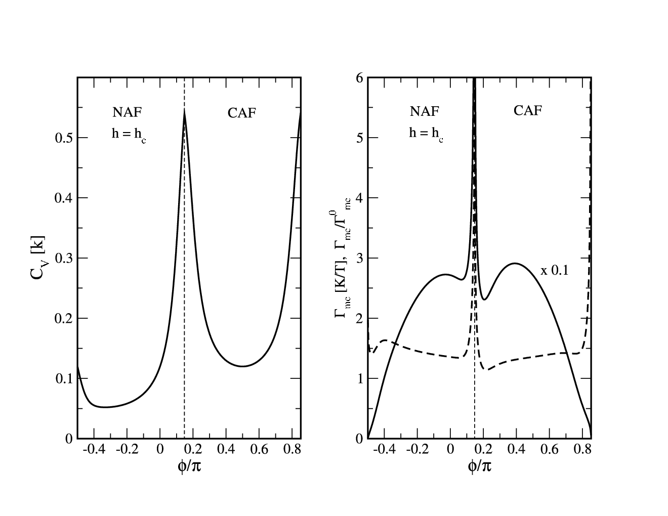
The same holds for the specific heat. In Fig. 16 (left panel) we show the peak value as function of frustration angle. Indeed the specific heat shows a strong enhancement for (CAF/NAF) and (CAF/FM) of considerable width in . This is in good qualitative agreement with the FTLM results for finite clusters presented in Fig. 9 (left panel). The anomaly at the FM/NAF boundary on the other hand is much smaller.
On the right panel of Fig. 16 the corresponding plot for the MCE is shown. The dashed line shows the bare MCE coefficient as function of . It is almost constant except at the phase boundaries where again a large, but much narrower peak appears. This is not immediately obvious since enters in the denominator of the expression for in Eq. (1). In fact on approaching the MCE slightly decreases, only very close to the value when the spin wave dispersion softens along the line – and equivalent ones in the BZ a very sharp spike appears. This is due to the fact that the spin wave softening leads to a stronger increase of the magnetization gradient (Eq. (42)) as compared to the increase of from Eq. (43). The full line in Fig. 16 (right panel) shows the normalized MCE. Aside from the phase boundaries where again sharp peaks appear it is largely determined by the behavior of the saturation field (Fig. 3) since the bare is roughly constant in .
Deep within the ordered phases the degree of enhancement of the MCE relative to an ideal paramagnet is chiefly controlled by the saturation field . The FTLM and LSW predictions are therefore in excellent qualitative agreement (c.f. Fig. 9 and Fig. 16). However, once again, finite size effects prevent the FTLM method from capturing the full extent of the anomalous enhancement of the MCE in the highly frustrated regions at the borders of the CAF phase. These may in practice be overestimated by LSW theory, since it takes no account of new non-magnetic phases stabilized by fluctuations.

None the less we can gain further insight into the strong enhancement of and the singular peak at in Fig. 16 within the LSW approach by expanding the spin wave energies of the fully polarized phase around the incipient ordering vector. Explicitly, for in the classical NAF sector we have
| (62) |
where is the distance from the NAF vector and is the excitation gap with the NAF critical field , The expansion coefficients are given by and . This expansion may be inserted into Eqs. (42, 43) and the integration performed approximately analytically. It is assumed that only modes with an energy contribute appreciably to the integral. In performing the integration one has to distinguish two cases: If one is within the NAF sector the second order coefficient is nonzero. If one is at the boundary to the CAF regime and the dispersion is determined by the mixed fourth oder coefficient .
Performing the integration in this (classical) limit one obtains the approximate expressions
| (63) | |||||
| (64) | |||||
In the corresponding quantum limit , both the heat capacity and the rate of change of magnetization with temperature have an activated behavior. However this cancels in between the numerator and denominator of Eq. (1) to give
| (65) |
regardless of the degree of frustration present in the model. We note that this is exactly the form predicted at a quantum critical point on the basis of scaling arguments Garst and Rosch 2005.
Returning to Eq. (63,64)—in the first case, inside the NAF sector, the divergence in the MCE for is only of a weak logarithmic type. However at the classical boundary to the CAF sector (which widens into the disordered regime due to quantum fluctuations) the singularity becomes a much stronger one essentially of inverse square root type. This is the reason that the MCE at shows a large anomalous peak as function of when crossing the NAF/CAF boundary. Because of the vanishing of the second order term in Eq. (62) the dispersion has a saddle point at leading to a large DOS of low energy spin waves for and therefore a stronger algebraic divergence of the MCE at appears. The same arguments hold for the CAF/FM boundary.
However a word of caution is appropriate. In our spin wave calculations we assumed that the classical magnetic phases are stable throughout the phase diagram. Strictly speaking this is not true. As indicated in Fig. 1 in the shaded sectors around the CAF/NAF and CAF/FM phase boundary quantum fluctuations lead to instability of magnetic order and select a different nonmagnetic order parameter, presumably staggered dimer Sushkov et al. 2001 and spin-nematic Shannon et al. 2006. While the broad features of our theory can be trusted, a truly quantitative theory for the nonmagnetic sectors would require to start from the proper order parameter and their associated elementary excitations. In real materials, sufficiently close to , the critical behavior of the MCE will also be sensitive to the details of interlayer coupling and magnetic anisotropy. Both refinements remain as an outstanding challenge.
It is also instructive to track the low to moderate field anomalies in as function of around the phase diagram. In Fig. 17 the maximum field and the field at which the MCE changes sign are plotted as function of frustration angle, normalized to the saturation field . While is rather constant throughout most of the range of angles, / shows considerable variation in . The two characteristic fields are again symmetric around =0.5 or =0 for the same reasons as explained above. Note that the overall double-minimum structure of / as function of prevents its use as a criteria to resolve the ambiguity of frustration angles that appears in zero-field thermodynamic considerations mentioned in Sec. III. It is obvious from the FTLM results in Fig. 10 (right panel), that the temperature dependence of the (normalized) MCE above is strongly suppressed as increases. This effect can also be understood from the LSW calculations. Approximating Eqs. (42,43) for small and large temperatures we obtain the ratio of the low and high temperature (normalized) MCE as function of :
| (66) |
As long as the field is not too far above there is still a considerable dispersion in and the above ratio is larger than one (Fig. 10), i. e. is -dependent. Once however the dispersion is negligible compared to the gap energy and the ratio in Eq. (66) approaches one, i. e. we recover the behavior of an ideal paramagnet.
A comparison between FTLM and LSW predictions of the temperature dependence of the MCE for fields safely above (in order to avoid the logarithmic singularity at ) is given in Fig. 18. There is a reasonable agreement in both magnitude and qualitative -dependence. Note however that the LSW approximation becomes unreliable when approaches / and too many spin wave modes are thermally excited.
VII Summary and Conclusion
We have investigated the magnetocaloric properties of the - model using the FTLM method for finite clusters and spin wave analysis starting from the classical magnetic structures. The one-magnon critical field or saturation field obtained from FTLM agrees well with the spin wave result. Finite size scaling results suggest that close to the CAF/FM boundary, the true critical field is determined by a two-magnon instability. This is consistent with the proposed existence of a spin nematic ground state in this parameter range Shannon et al. 2006.
Both FTLM and spin wave results predict a strong enhancement in the low temperature specific heat at the saturation field when the frustration angle crosses the phase boundaries. This may be explained by the large degeneracy of low lying states in these regions. At a constant intermediate field the specific heat exhibits a double peak structure around the NAF/CAF boundary. The entropy and specific heat show only moderate field dependence below the saturation field . This feature may already be understood in a mean field approach where the entropy is strictly constant for all .

Likewise the strong enhancement of the MCE just above the saturation field was investigated. In the FTLM results, the MCE was enhanced by up to a factor ten relative to an ideal paramagnetic (at temperatures small compared to the energy scale ). Surprisingly, the largest enhancement (from FTLM, relative to an ideal paramagnet) does not occur at the CAF/NAF boundary, but deep within the magnetically ordered sectors. This can be understood in terms of the anomalous enhancement of the specific heat in the frustrated regions, which enters into the denominator of the MCE (c.f. Eq. (1)).
The overall dependence of the MCE enhancement ratio reflects that of the saturation field. This is also true for the spin wave results. There, in addition, the enhancement is sharply peaked on the CAF/NAF boundary appears. This is due to the change of the field-scaling behavior above the critical field from logarithmic to inverse square-root when the boundary is crossed. This feature is due to the appearance of Goldstone modes along a line in the BZ when has it critical value. The MCE enhancement may also be directly seen from the isentropics or adiabatic temperature curves which exhibit a large slope above the saturation field.
Below the saturation field the results of the FTLM is strongly constrained by finite size effects, however the spin wave analysis provides considerable insight into the systematic properties of the MCE. In absolute terms the MCE is very small—in fact much smaller than the paramagnetic value. This is a direct consequence of magnetic order, and can easily be understood from the mean field picture of a canted Néel state, for which entropy is constant as a function of field. The spin wave theory, however, predicts a flat maximum in the MCE at low fields, followed by a sign change for subcritical fields. These features are present throughout the phase diagram and the characteristic fields are moderately -dependent with a double-minimum structure. For this reason it is not likely that these low-field MCE features are useful in the determination of the frustration ratio.
Considerably above the critical field the temperature dependence calculated from FTLM and spin wave theory show reasonable agreement. At temperatures of the order of the enhancement of the MCE is substantially reduced and the behavior of the system crosses over to that of an ideal paramagnet.
The most pronounced discrepancies between FTLM and spin wave analysis appear at the classical phase boundaries. As explained above this may be well understood in terms of the absence or presence of low lying collective modes. While the former method underestimates the MCE anomalies at the phase boundaries, the latter overestimates them—in fact it predicts a singular behavior. A more advanced analytical treatment would have to take into account the quantum nature of the ground state around these boundaries, i. e. stacked dimer () or spin nematic () and the proper associated excitation spectrum.
The present analysis provides some interesting predictions for the experimental investigation of the class of layered perovskites discussed in the introduction. Specifically we give detailed values for the possible saturation fields which should be easily accessible experimentally for SiO4 and PO4 vanadates. According to Fig. 4, these critical fields can be used to resolve the ambiguity in parameterizing the model from its low-field susceptibility and heat capacity, far more cheaply than, e.g. neutron scattering. Furthermore we predict a genuine sign change in the MCE for subcritical fields which should be accessible to experiment.
So far as practical applications—for example in cryogen free cooling—are concerned, the goal is to achieve as large a magnetocaloric effect as possible, at as low a field as possible. Here compounds not too far from the phase boundaries FM/NAF and CAF/FM are the most promising because they combine a significant MCE enhancement with very moderate saturation fields. A detailed treatment of entropy as a function of magnetic field in the nematic phase occurring on the CAF/FM border remains an open challenge. However the high density of low energy excitations and low saturation field of this phase means that it looks a priori very promising for magnetothermal applications.
Acknowledgements.
The authors are pleased to thank Tsutomu Momoi, Philippe Sindzingre and Matthias Vojta for helpful discussions. N.S. acknowledges support under EPSRC Grant No. EP/C539974/1. P.T. acknowledges support by Deutsche Forschungsgemeinschaft under SFB 463.Appendix A Moment derivatives
Here we give the explicit expressions of the moment derivatives () which are needed for the mean field calculation of the magnetocaloric coefficient:
| (67) | |||||
| (68) |
Where the determinant D is defined by and the coefficients ( or , or ) and are given by
| (69) | |||||
and likewise
| (70) | |||||
Appendix B Matrix form of the Hamiltonian
In this appendix we give the explicit matrix form of the Hamiltonian in Eq. (51) for the NAF structure which is bilinear in bosonic spin fluctuation operators. It can be written as
where the constant term (arising from spin commutation relations) ensures that the zero point energy is negative. Using a simple coordinate rotation, we can reduce this matrix to a block diagonal form with two diagonal blocks given by
We can then solve each of the blocks using a separate, standard, Bogoliubov transformation to obtain the diagonalized Hamiltonian in terms of NAF spin wave modes as used in Eq. (55).
Explicitly the complete transformation is given by
| (83) |
where is the branch index. The coefficients and of the transformation may be obtained by direct insertion and the requirement that the off-diagonal bilinear terms in the transformed operators vanish identically. Alternatively the equations of motion for the may be set up and required to describe free motion with spin wave energy . Both methods lead to the same condition on the coefficients given by
| (84) |
Using the representation , , one obtains the two branches () of the solution with
| (85) |
The prefactor of the remaining diagonal bilinear term in the transformed Hamiltonian gives the spin wave energies of Eq. (56).
References
- Misguich and Lhuillier (2004) G. Misguich and C. Lhuillier, in Frustrated Spin Systems, edited by H. T. Diep (World Scientific, 2004).
- Shannon et al. (2004) N. Shannon, B. Schmidt, K. Penc, and P. Thalmeier, European Physical Journal B 38, 599 (2004).
- Shannon et al. (2006) N. Shannon, T. Momoi, and P. Sindzingre, Physical Review Letters 96, 027213 (2006).
- Millet and Satto (1998) P. Millet and C. Satto, Materials Research Bulletin 33, 1339 (1998).
- Melzi et al. (2000) R. Melzi, P. Carretta, A. Lascialfari, M. Mambrini, M. Troyer, P. Millet, and F. Mila, Physical Review Letters 85, 1318 (2000).
- Melzi et al. (2001) R. Melzi, S. Aldrovandi, F. Tedoldi, P. Carretta, P. Millet, and F. Mila, Physical Review B 64, 024409 (2001).
- Kaul (2005) E. Kaul, Ph.D. thesis, Technische Universität Dresden, Dresden (2005).
- Kini et al. (2006) N. S. Kini, E. E. Kaul, and C. Geibel, Journal of Physics: Condensed Matter 18, 1303 (2006).
- Warburg (1881) E. Warburg, Annalen der Physik und Chemie 13, 141 (1881).
- Pecharsky and Gschneidner (1999) V. K. Pecharsky and K. A. Gschneidner, Journal of Magnetism and Magnetic Materials 200, 44 (1999).
- Tishin et al. (1999) A. Tishin, K. A. Gschneidner, and V. K. Pecharsky, Physical Review B 59, 503 (1999).
- Zhitomirsky (2003) M. E. Zhitomirsky, Physical Review B 67, 104421 (2003).
- Zhitomirsky and Honecker (2004) M. E. Zhitomirsky and A. Honecker, Journal of Statistical Mechanics: Theory and Experiment 2004, 07012 (2004).
- Zhitomirsky and Tsunetsugu (2005) M. E. Zhitomirsky and H. Tsunetsugu, Progress of Theoretical Physics Supplement 160, 361 (2005).
- Misguich et al. (2003) G. Misguich, B. Bernu, and L. Pierre, Physical Review B 68, 113409 (2003).
- Schmidt and Thalmeier (2005) B. Schmidt and P. Thalmeier, Physica B: Condensed Matter 359-361, 1387 (2005).
- Schmidt et al. (2006) B. Schmidt, N. Shannon, and P. Thalmeier, Journal of Physics: Conference Series 51, 207 (2006).
- (18) M. Skoulatos, J. P. Goff, M. Enderle, and N. Shannon, in preparation.
- Jaklic and Prelovsek (2000) J. Jaklic and P. Prelovsek, Advances in Physics 49, 1 (2000).
- Kaul et al. (2004) E. E. Kaul, H. Rosner, N. Shannon, R. V. Shpanchenko, and C. Geibel, Journal of Magnetism and Magnetic Materials 272-276, 922 (2004).
- Honecker (2001) A. Honecker, Canadian Journal of Physics 79, 1557 (2001).
- Jackeli and Zhitomirsky (2004) G. Jackeli and M. E. Zhitomirsky, Physical Review Letters 93, 017201 (2004).
- Sindzingre (2004) P. Sindzingre, Physical Review B 69, 094418 (2004).
- Garst and Rosch (2005) M. Garst and A. Rosch, Physical Review B 72, 205129 (2005).
- Kalva et al. (1976) Z. Kalva, I. Veltrusky, and G. Kozowski, Physics Letters A 57, 75 (1976).
- Kalva et al. (1978) Z. Kalva, I. Veltrusky, L. Biegala, and G. Kozlowski, Czechoslovak Journal of Physics 28, 183 (1978).
- Sushkov et al. (2001) O. P. Sushkov, J. Oitmaa, and Z. Weihong, Physical Review B 63, 104420 (2001).