The Quantum de Laval Nozzle: stability and quantum dynamics of sonic horizons in a toroidally trapped Bose gas containing a superflow
Abstract
We study an experimentally realizable system containing stable black hole-white hole acoustic horizons in toroidally trapped Bose-Einstein condensates - the quantum de Laval nozzle. We numerically obtain stationary flow configurations and assess their stability using Bogoliubov theory, finding both in hydrodynamic and non-hydrodynamic regimes there exist dynamically unstable regions associated with the creation of positive and negative energy quasiparticle pairs in analogy with the gravitational Hawking effect. The dynamical instability takes the form of a two mode squeezing interaction between resonant pairs of Bogoliubov modes. We study the evolution of dynamically unstable flows using the truncated Wigner method, which confirms the two mode squeezed state picture of the analogue Hawking effect for low winding number.
I Introduction
The idea of analogue gravity Barcelo2006, which includes the possibility of observing the analogue of the Hawking effect in fluid systems exhibiting sonic horizons, was first put forward by Unruh Unruh1981. In that paper, using an analysis similar to Hawking’s original analysis for cosmological black holes Hawking1974; Hawking1975, Unruh showed an acoustic black hole should emit sound waves with a Planckian spectrum at the Hawking temperature
| (1) |
where is the surface gravity at the black hole horizon and is the speed of sound at the horizon. The derivation required the quantization of a scalar field propagating in a classical fluid, analogous to a classical gravitational field. In Bose-Einstein condensates (BECs) long wavelength excitations propagate hydrodynamically, giving a direct analogue model in a system where the Hawking temperature is relatively large Barcelo2003b, and potentially measurable using recently proposed schemes based on Raman spectroscopy Schutzhold2006, or parametric resonance Modugno2006.
Even in the ultra-cold regime where BECs occur, an extremely low temperature and low losses are both desirable features of any experimental setup to test analogue Hawking radiation in BECs, since it is inherently a delicate and weak signal. One way to realize a sonic horizon in a trapped BEC without any outcoupling is by setting up a persistent supercurrent in a toroidal trap with “bumps” in the trapping potential. The bumps act like constrictions, creating a de Laval nozzle LandL type configuration (Fig. 1). The experimental realization of a toroidal magnetic trap for ultracold atoms, first demonstrated by using two current-carrying loops Sauer2001, has since been developed using magnetic waveguides Gupta2005, a microchip trap Crookston2005 and a four loop configuration Arnold2006. The requisite bumps could be introduced optically by a detuned laser shining through an appropriately patterned mask Tung2006a.

While there exist previous theoretical studies of de Laval nozzle geometries in the context of acoustic black holes, both for classical fluids Sakagami2002; Furuhashi2006 and for BECs Visser2002; Barcelo2003b, the analyses in these studies are either classical or semiclassical in nature. Previous investigations of acoustic black hole geometries Barcelo2003b; Visser2002; Leonhardt2003 have focused on regimes where both the hydrodynamical and geometric acoustics descriptions for a BEC apply, so that the semiclassical WKB method can be applied to calculate the Hawking temperature in close analogy with the gravitational derivation Hawking1974; Hawking1975; Unruh1981; Visser1993. In particular, flows are treated as hydrodynamic, and the effects of the trap are neglected through some form of local density or WKB approximation. This is understandable given the conditions under which Hawking first discovered the effect, but our primary interest are quantum effects which have also been studied for other BEC acoustic horizon scenarios Garay2001; Visser2002; Barcelo2003b; Leonhardt2003; Leonhardt2003b; Giovanazzi2004.
In this work, we consider a quite different regime where hydrodynamics is valid only for the low energy modes, whereas geometric acoustics is only valid in the limit of high winding number. The system of interest is in the region of parameter space where hydrodynamics and geometric acoustics approximations are not usually applicable, but where progress can be made with more detailed numerical analysis.
We introduce and analyze a system which exhibits an acoustic black hole and white hole horizon in a trapped BEC, formed by two de Laval nozzles in a toroidal geometry. Under the conditions of steady flow this configuration represents the simplest stable de Laval geometry for a Hamiltonian BEC system, and has some appealing properties for studying the analogue Hawking effect. In particular, it has a discrete excitation spectrum and periodic boundary conditions. Our primary aims are to find stationary solutions of the Gross-Pitaevskii equation for this system, and to investigate their stability and quantum dynamics.
II Quantum de Laval Nozzle
A weakly interacting Bose gas trapped in a one dimensional potential at zero temperature is well described by the Gross-Pitaevskii equation Dalfovo1999; Garay2001
| (2) |
where the effective one dimensional interaction strength is and is the usual -wave interaction parameter. The reduction to one dimension assumes the transverse wavefunction is in the harmonic oscillator ground state of toroidal trap: , for which we require , where is the transverse trapping frequency. The dynamics become effectively one dimensional in this regime since the transverse motion is frozen out by the large energy required to excite transverse modes. The -wave scattering description remains valid provided the scattering length is much smaller than the transverse dimension so that the scattering remains effectively three dimensional Morgan2002a. The wavefunction can be written as a macroscopic order parameter
| (3) |
with current density
| (4) |
and velocity . In density-phase variables the system is governed by the equations of motion
| (5) |
and
| (6) |
When the interaction term dominates, the density varies slowly, and the Laplacian term (quantum pressure) can be dropped; then the last equation can be takes the form of Euler’s equation
| (7) |
and we recover the classical isentropic flow equations. Combining (5) and (7), one can derive the nozzle equation LandL; FluidMechYih.
| (8) |
relating variations of the potential and the flow velocity. The physical consequences of this form of the nozzle equation are as follows (refer to Fig. 1): Sonic flow () is only permitted where , that is at the waist of the nozzle. For subsonic flow (), when is negative/positive the velocity is decreasing/increasing. Conversely for supersonic flow, when is negative/positive the velocity is increasing/decreasing. Therefore, if the flow is subsonic on approach to the nozzle waist, becoming sonic at the waist, it becomes supersonic on exiting the waist, and conversely for an approaching supersonic flow.
To achieve transonic steady flow in a toroidal geometry, two de Laval nozzles are required in tandem, the flow becoming supersonic at the waist of the first, and then subsonic at the waist of the second. This configuration corresponds to the formation of both a black and white hole horizon. To implement such a geometry we consider an external potential of the form
| (9) |
which has periodicity 2 over the interval , which is periodic for the toroidal geometry. For a BEC confined by such a potential, the stationary states are found by solving the time-independent Gross-Pitaevskii equation subject to phase quantization. Since, as we will see below, the solutions exhibit strong modifications to hydrodynamic behavior, we refer to this configuration as the quantum de Laval nozzle (QdLN).
We wish to study currently realistic or potentially achievable parameters. Toroidal ultra-cold atom waveguides have been developed by several groups Gupta2005; Arnold2006. We take as nominal values those of the recent experiments of the Stamper-Kurn group Gupta2005. The experiments typically consist of 87Rb atoms held in a toroidal trap with transverse frequency , and radius which gives an azimuthal length and a transverse harmonic oscillator dimension . Typical winding numbers are estimated by assuming that the circulation velocity is constant and assuming that the gas fills the entire perimeter of the toroid (which is not the case in the experiment). This leads to the estimate , which for the circulation period of Ref. Gupta2005 () gives which is quite large. Constructing stationary solutions for the quantum de Laval nozzle for these exact parameters presents a major computational challenge as it is necessary to resolve phase variations of the wavefuction on a very small scale, however we note that the condensates in this experiment are launched into the toroid and do not form periodic stationary solutions. In theoretical work existing in the literature more modest winding numbers have been considered: Garay2001. In this work we will examine the stability of a similarly modest range of winding numbers in detail, and also for comparison we include .
III Stationary states
In this section we find stationary solutions for the QdLN using the Gross-Pitaevskii equation and compare the results with hydrodynamic and perturbative approaches.
It is convenient to normalize the condensate wavefunction to the single particle form in what follows, so that hereafter describes the total effective nonlinearity for condensate atoms. For steady state flow we take the one dimensional stationary solution of the form
| (10) |
If we take the stationary solution of (5) and (6) using (10), and take the fixed current condition, we can write , ,
| (11) |
Solutions to this nonlinear equation then allow us to reconstruct the wavefunction by specifying:
| (12) | |||||
| (13) |
Solutions must also satisfy the phase quantization condition
| (14) |
for an integer winding number given by .
III.1 Hydrodynamic solutions
When the interactions dominate the density varies slowly so we can invoke the hydrodynamic approximation and drop the Laplacian term. In this case (11) can be written as a cubic, either in terms of the density:
| (15) |
or in terms of the velocity:
| (16) |
For the case where the flow is zero, there is one non-trivial solution to (15)
| (17) |
The chemical potential is , which yields the density
| (18) |
On the other hand, for the case where there is non-zero flow (), we find solutions using (16) since the equations have a simpler form in this case. The solutions are conveniently separated by the discriminant of the cubic Abram
| (19) |
Transonic configurations exist when there are two real positive solutions, which occurs when for all . Since the negative semi-definite character of imposes the constraint . We can express these solutions analytically as:
| (20) | |||||
| (21) |
with
| (22) |
Note is the subsonic branch, whereas is the supersonic branch.
A continuous, single valued transonic solution can be constructed when the two positive solutions coincide at the horizon, which we take to be . This occurs when . At the horizon (ie. the maximum of the potential acts as the waist of the de Laval nozzle), so rearranging (19) we find the condition for transonic flow is given by the critical chemical potential
| (23) |
Note for we have and the flow is unstable.
We can find a transonic solution by taking the chemical potential so that there is a crossover from the subsonic to supersonic branches at the horizon: . The transonic solution is then constructed by joining the subsonic () and supersonic () solution branches. Without loss of generality, we take the subsonic branch to span the interval , with the supersonic branch in the interval . Consistent solutions with integer winding number are found by iterating the hybrid solutions and the constraints to find the appropriate conserved current . The resulting stationary solution is fully determined by the parameters , and .
III.2 Perturbation theory
Although we have the analytical solutions of the hydrodynamic theory it is useful to adopt a perturbative approach which has the advantage of giving simple and reasonably accurate solutions at first order in powers of , where is the zeroth order chemical potential. We have chosen our potential so that we can choose the unperturbed problem as the homogeneous solution for , with critical flow so that everywhere.
At any order the solutions must satisfy the set of equations
| (24) | |||||
| (25) | |||||
| (26) | |||||
| (27) |
At zeroth order, the potential free equations satisfied by the unperturbed variables are
| (28) | |||||
| (29) | |||||
| (30) | |||||
| (31) |
In solving the cubic we find solutions . Only the positive flow solutions are physical and their coalescence at zeroth order is helpful at higher order where the solutions break the parity symmetry of the potential.
At zeroth order the solutions can expressed in terms of the winding number as , , , and . Since we are going to require this imposes the condition
| (32) |
for the validity of the perturbation series. We introduce the rescaling , to obtain the equations
| (33) | |||||
| (34) | |||||
| (35) | |||||
| (36) |
The repeated solution at zeroth order means we have to use a perturbation series in powers of Bush, so we assume an expansion of the form and similarly for the other variables. We can obtain consistent solutions to Eqs. (33–36) up to which give a good qualitative description of the solutions and are quite accurate for a wide range of parameters.
Terms in the expansion of (33) of order cancel, and the equation is
| (37) |
Substituting the series into (34) gives which is not surprising, and in fact . The subsonic and supersonic solutions are automatically matched at the acoustic horizon by choosing , whereby the supersonic region is , coinciding with our previous hydrodynamic treatment.
Returning to dimensioned variables, the first order solutions for the quantum de Laval nozzle are
| (38) | |||||
| (39) |
with and . These expressions give a good qualitative description of the Gross-Pitaevskii solutions, and are typically very close to the full hydrodynamic solutions (see Fig. 2). As expected, the differences are more apparent with increasing corresponding to a more important quantum pressure term, and with increasing distance from the sonic horizons.
III.3 Solutions of the Gross-Pitaevskii equation
We now use the transonic solution to the hydrodynamic problem (Sec. III.1) as a starting point to finding the stationary solutions of the Gross-Pitaevskii equation (GPE). The full numerical solutions exhibit “ripple” structures in regions where the quantum pressure term becomes important, in particular, in the region of supersonic flow downstream of the black hole acoustic horizon.
In order to find stationary solutions we use constrained optimization. Imaginary time evolution is not feasible in this case because we are interested in stationary states which are excited into circular motion relative to the ground state. We formulate the problem as the the minimization of the Gross-Pitaevski functional for a fixed nonlinearity , potential depth and current , subject to a phase quantization constraint in terms of a fixed winding number . The problem is recast as the set of algebraic equations:
The phase circulation constraint ensures the wavefunction is everywhere single-valued.
The solution for our vector of unknowns is found by Levenberg-Marquardt optimization Levenberg1944a; Marquardt1963a in MATLAB using the hydrodynamic solution as the initial condition . The unit of energy for this system which we will use to display our results is .


To consider some examples we use a potential with , and show solutions for winding numbers (Fig. 2) and (Fig. 3). In each case, the full hydrodynamic, first order perturbation theory and GPE solutions are shown, as well as the flow velocity and speed of sound for the GPE stationary solution, and the location of the acoustic black hole (BH) and white hole (WH) horizons. The ergoregion () is given approximately by the right hand region . By construction, in the hydrodynamic case, the black hole horizon occurs at , whereas the white hole horizon occurs at .
In principle we might expect to be able to vary the winding number and potential depth to find a continuous range of transonic solutions for the QdLN. This is the case, for example, for the toroidal system considered by Garay et al. Garay2001, where for a given a stability diagram over a continuous range of and was mapped out. In fact we find that for the QdLN the total nonlinearity is not a free parameter of the solutions – it is uniquely determined for a given . This is physically reasonable because sets the flow velocity and the nonlinearity determines the speed of sound, and the two must be equal at the sonic horizons.
We can easily find a very accurate relation between nonlinearity and winding number using the zeroth order perturbation theory: . We should expect deviations from this relationship for low winding number due to the importance of the quantum pressure term, however we find they are very small. Numerically we find for the GPE solutions that varies according to this quadratic law and depends only very weakly on . For the values of used in this paper the behavior is essentially independent of and shows a maximum deviation from the zeroth order perturbation theory result of order , occurring at our lowest winding number, .
Qualitatively, the main departure of the hydrodynamic solutions from first order perturbation theory is a loss of parity: the increasingly important interaction energy eventually lifts the antisymmetry of ; such differences are more pronounced for low winding number.
IV Quasiparticles and stability
We will now determine the stability of the GPE stationary solutions by finding their Bogoliubov excitation spectra for a wide range of potential depths and winding numbers. For unstable configurations the standard Bogoliubov analysis is insufficient, and we use the theory of Leonhardt et al. Leonhardt2003 to obtain the correct normalizable Bogoliubov modes. These modes show some interesting localization properties with respect to the acoustic horizons, and will be used to construct Bogoliubov vacuum states when we come to dynamical simulations in Sec. V.
IV.1 Normalizable Bogoliubov modes
The linear excitations of the condensate are described by the Bogoliubov-de Gennes (BdG) equations Morgan1998; STR. Consider a solution with small oscillations around a stationary state
| (40) | |||||
where and are the amplitudes for the oscillations and is normalized to unity in what follows. For the quantum field, these quantities are replaced by the bosonic annihilation and creation operators for the excitations, given by and respectively, with . is the solution to the time-independent GPE given by (2). To obtain the correct physical modes it is necessary to introduce the operator
| (41) |
which projects orthogonal to the condensate. Introducing projectors appropriately and substituting the Bogoliubov expansion into the time-dependent GPE and while only keeping terms linear in and yields the modified BdG equations
where the operator is given by
and the Gross-Pitaevskii operator is
| (50) |
The stationary solution satisfies . The solutions to this equation are the eigenvalues , and the normal modes of the system.
The orthogonality and symmetry relations are fixed by the requirement that the many body Hamiltonian for the interacting Bose gas is diagonal (to quadratic order) in quasiparticle operators and that the transformation to quasiparticles preserves the commutation relations.
The operator is not Hermitian so that complex eigenvalues are allowed, corresponding to dynamical instabilities of the system. It is straightforward to show that the modes with complex eigenvalues have zero norm Fetter1972 and cannot therefore be associated with bosonic operators in the field expansion (40). However, following Leonardt et al. Leonhardt2003, it is still possible to construct normalizable modes for the unstable modes by the construction:
where and are the eigenvectors associated with the unstable positive and negative energy eigenvalues respectively. Note that due to the symmetries of (IV.1) we have . Hereafter we use and for the full set of orthonormal modes. The quadratic Hamiltonian for the stable modes takes the standard form for independent harmonic oscillators. The creation and annihilation operators for the new modes satisfy the commutation relations for bosonic operators, but show up as non-diagonal terms in the Hamiltonian subspace for the dynamically unstable modes as Leonhardt2003
| (65) | |||||
where the sum is taken over only the dynamically unstable modes, and where is the annihilation operator and the creation operator corresponding to the normalizable modes (IV.1) and (IV.1). For stable modes the hamiltonian reduces to the usual diagonal Bogoliubov form . Dynamically unstable modes are therefore associated with non-degenerate parametric amplification QO, which leads to growth in the unstable modes at the expense of the condensate mode. For short time dynamics, the complex eigenvalue will generate exponential growth in each unstable mode. It is this effect that has been suggested to provide the closest analogy with the Hawking effect for BECs Garay2001; Leonhardt2003. However, this picture neglects higher order interactions that may be present in the full Hamiltonian, and therefore is likely to fail for dynamics on long time scales. We will investigate this further in Sec. V.
IV.2 Stability and mode structure
For a dynamically unstable configuration, we construct normalizable modes using the procedure outlined in Sec. IV.1. We additionally sort the eigenvalues in ascending order by and label the modes accordingly.

Figure 4 shows the eigenvalue spectrum for the first few modes with and two different values of : (a) ; and (b) . While both cases have negative eigenvalues, indicating energetic (Landau) instabilities due to non-zero flow, only case (b) exhibits dynamical instabilities also. Following the theory of the previous section, the onset of a dynamical instability is associated with a pair of modes (labelled by and say) with complex eigenvalues that satisfy . In particular, case (b) indicates that modes 1 and 6 are unstable with .

Figure 5 shows the stability diagram for the QdLN that results by performing the diagonalization for a range of parameters, and . For each point we have calculated the maximum of the absolute value for the imaginary part of all eigenvalues. The essential features we observe are: (i) there are regions exhibiting dynamic instabilities; (ii) these regions become narrower and smaller in magnitude, but more closely spaced for larger values of the winding number , whereas they become broader and larger in magnitude as the potential depth increases.


In Fig. 6 we show the corresponding mode functions and that result from the solutions of the BdG equations for the parameters and , which has a dynamical instability for the modes , . We note, although not shown here, the mode functions for and (dynamically stable) are very similar to the case.
The mode functions exhibit a rich structure for the low energy modes, not least being the sort of “localization” of modes that is associated with the acoustic black hole geometries. In particular, for modes , is localized in the region , which corresponds to the supersonic region, whereas is localized in the region , corresponding to the subsonic region. For modes we find the reverse is true in general, although the localization occurs to a lesser extent. Modes , (the dynamically unstable modes) indicate a crossover between these two regimes. In Fig. 7 we show the average position of the quasiparticle modes for two unstable cases for comparison. The mean quasiparticle position for each mode is calculated as Isoshima2003 , where with defined similarly, and . We note that the negative energy modes (1-3 for and 1-5 for ) are always located significantly inside the sonic horizon , while higher energy modes become located nearer the horizon.
V Dynamics
To investigate the time dynamics of the QdLN we will use the stationary states as our starting point for quantum field theory simulations using the truncated Wigner method. We will compare the quasiparticle population dynamics in both stable and unstable regimes. First we briefly discuss the connection between our Bogoliubov analysis and the analogue Hawking effect.
V.1 Two-mode Bogoliubov model
The interaction Hamiltonian for a pair of dynamically unstable modes with , and with is
| (66) |
which describes the formation of a two-mode squeezed state. By finding the time evolution for the two mode density matrix according to and averaging over the negative energy mode we obtain the density operator for the positive energy mode
| (67) |
a thermal state with mean occupation . We thus have a loose analogy with the Hawking effect: pairs of quasiparticles can be produced with no energy cost, such that one quasiparticle enters the negative energy state which is located inside the supersonic region (for our case in Fig. (6) this is mode 1), and the other is promoted to positive energy (mode 6), which is centered much closer to the horizon. Tracing over the negative partner gives a thermal state for the postive energy mode. This connection has been pointed out previously Leonhardt2003, but to our knowledge it has not been confirmed for the trapped Bose gas using analysis of the GPE as we are able to do here (see Fig. 9). However, we note that the analogy with the gravitational Hawking effect is incomplete, as may be seen from the time dynamics of the positive energy mode occupation number. A more direct Hawking analogue would generate a time independent multimode thermal emission spectrum, whereas here we have an exponentially growing, single mode emission.
Thus far, we have found the elementary excitations for the QdLN and found that this indicates dynamically unstable configurations for certain sets of parameters. In order to verify that such configurations do indeed lead to exponential growth in the unstable modes, we consider the dynamics of the system. To do this we use the truncated Wigner method to perform short time simulations of the full interacting quantum field theory describing the trapped Bose gas.
V.2 Truncated Wigner method
The Wigner representation provides a symmetrically ordered formalism for phase space simulations of quantum field theory. Symmetrically ordered operator averages are computed by ensemble averaging many classical field trajectories. The truncated Wigner method Steel1998; Sinatra2000; Sinatra2001; Sinatra2002; SGPEI; SGPEII; Polkovnikov2003 involves neglecting intractable third order derivatives in the equation of motion for the Wigner distribution. The method then reduces to numerically evolving a multimode classical field using the GPE (2) Steel1998. The theory differs from pure mean field theory in that statistical fluctuations in the initial state reproduce quantum fluctuations in the observables extracted by ensemble averaging. The method is known to be accurate for short evolution times Steel1998. In the low temperature regime , the initial field is given by
| (68) |
where is a stationary state of the GPE (for our purposes, the transonic solutions of the QdLN), and where and are the Bogoliubov mode amplitudes of the system. The complex random variables are constructed as , where are real, normal Gaussian variates with and , and is the thermal quasiparticle occupation. The notation represents the stochastic average over many samples of . In this work we restrict our attention to the zero temperature case to investigate the stability and dyanamics of our stationary solutions in the presence of vacuum fluctuations.
We expect the details of the quantum dynamics to depend sensitively on any instabilities, and indeed, according to the two mode model, instabilities can generate squeezing. We use the quasiparticle occupation numbers to look for confirmation of this effect in our simulations. Dynamically, the Bogoliubov amplitudes can be extracted from the classical field as
| (69) |
which we use to monitor the populations during our simulations. The quasiparticle number in each mode is then
| (70) |
where the bar indicates an ensemble average over many Wigner trajectories.
In any simulations we must use a restricted basis, and our GPE evolution is numerically projected at each time step to ensure that the system remains in the low energy subspace determined by our energy cut-off. Formally we are using the projected GPE (PGPE) Davis2001b to ensure consistent evolution of our restricted phase space. For the evolution of the PGPE we have used the fourth-order Runge-Kutta in the interaction picture (RK4IP) algorithm BMCDThesis, adapted to project into the low energy subspace defined by our momentum cutoff at Davis2002. For the simulations presented here we have use condensate atoms, and modes for the system in the low energy subspace, corresponding to a dimensionless momentum cutoff . For all simulations we have used a time step for the RK4IP algorithm ensuring the change in total field normalization during each trajectory was .
V.3 Results

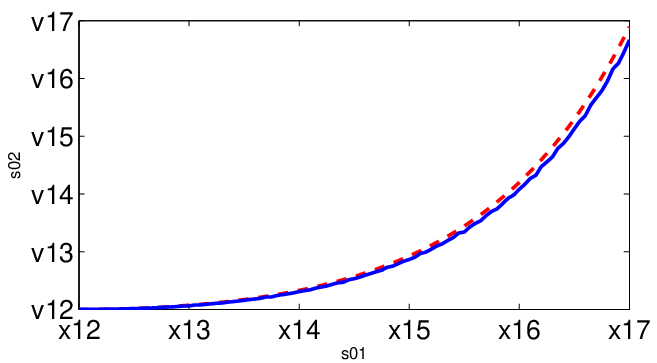

For a winding number of , we have carried out time dynamical simulations for 40 trajectories using the truncated Wigner method. The ensemble averaged quasiparticle mode occupations have been calculated for two cases (refer to the stability diagram in Fig. 5): (i) For the stable case , the quasiparticle modes remain unnocupied during the interval . This confirms the stability of the system to the extent possible given that our GPE stationary state with vacuum noise is only an approximation to the true many body stationary state. (ii) Fig. 8 shows the populations for the unstable case, . In the latter case, modes , are unstable, and we observe exponential growth in these modes. The growth is seeded by the quantum vacuum fluctuations in the initial state and confirms the expectation that the system obeys the Hamiltonian (65) for a non-degenerate parametric amplifier at short times. Note that the mean quasiparticle occupation for modes is also negligible compared with . In Fig. 9 we plot the population in the positive energy mode of the unstable pair, , which is seen to be in close agreement with the dynamics expected from the Bogoliubov theory of Sec. IV.
We have also investigated the behaviour of the dynamically unstable configuration for longer times. Single trajectory results for a simulation time of are shown in Fig. 10. Here we observe growth in the unstable modes (, ) until where there is a peak in the mode populations, followed by a decay of occupation numbers. Therefore the system undergoes a period of excitation followed by an apparent return to the initial unexcited state. This is also evident in the coordinate space density plots for the same simulation given in Figs. 11 (a) and (b). In particular, plot (a) shows large scale density fluctuations for . Plot (b) shows the density relative to the initial state, from which it is clear that the density fluctuations are localised in the region corresponding to the supersonic region for the system. It seems plausible that such excitations and revivals should continue to repeat, which would result in a “ringing” type excitation of the condensate. However, due to the significant computational time required, we did not check this prediction.
The recurrence of the system is evidently due to nonlinear mode mixing, which is neglected in the BdG analysis. In particular, the back-reaction of quasiparticle modes on the condensate should become significant for large mode occupations. Moreover, the topological constraint imposed by the periodicity of the system (ie. by a fixed winding number) means that the decay of circulation for the superfluid flow is forbidden. Evidently the decay channel for this instability is inhibited. The system cannot reach a quasi-stationary state corresponding to a different value of , without a corresponding change in and the damping of topological charge; one mechanism for this process would be soliton shedding, but we have not observed this in our simulations of this system.


We also investigated the dynamics for the higher winding number . In particular, we have examined two flows, which are (i) the dynamically stable (according to the BdG analysis) flow, ; and (ii) the dynamically unstable flow . We briefly summarize the results for this case as we have found it to be typical of high winding number behaviour. From our ensemble averaged time dynamics carried out in a similar manner to the previous cases, we found (1) that linear stability, evidenced by time-independent vacuum quasiparticle population, was confirmed for short time quantum dynamics; (2) for the unstable configuration, chaotic multimode dynamics is evident in the otherwise stable time interval, in particular, we did not observe simple two mode squeezing dynamics of the kind seen for . This behaviour is not unexpected since for the higher winding number, the effective nonlinearity required is very large (recall from the perturbation theory of Sec. III the nonlinearity scales with the square of winding number). In our quantum dynamical simulations elementary excitations interact with each other, giving rise to Landau-Beliaev damping Pitaevskii1997; Giorgini1998, and this effect is more pronounced at higher nonlinearities.
VI Conclusions
We have introduced and analyzed the quantum de Laval nozzle, a toroidal geometry for a BEC that exhibits both a black and white sonic horizon. Using hydrodynamic theory we have found transonic solutions, which we used to find transonic stationary solutions of the Gross-Pitaevskii equation. The qualitative properties of the GPE solutions are well described by hydrodynamic perturbation theory at lowest order. The system has broad dynamical instabilities for certain values of the winding number and potential depth .
We constructed normalizable Bogoliubov modes for the dynamical instabilities, which couple modes of positive and negative energy. This analysis leads to a two mode squeezing Hamiltonian term corresponding to non-degenerate parametric amplification, which leads to exponential population growth of unstable mode occupation with time – this represents the closest analogy with the Hawking effect for our trapped quantum system.
To analyze this picture further, we have investigated the dynamics of several configurations using the truncated Wigner method which from an analogue model point of view includes the effects of nonlinear interactions between modes and back reaction. For low winding number we observe non-degenerate parametric amplification type dynamics at the instability, confirming the two-mode Bogoliubov model validity, while for the stable configuration there is negligible growth in all modes.
From the stability analysis, we note for large winding number solutions: (i) the number of unstable regions increases, and they become narrower; (ii) the nonlinearity increases so that the system approaches the hydrodynamic regime; and (iii) short wavelength negative energy modes, for which the geometric acoustics approximation may be valid, increase in number. The combination of these effects indicates that in the limit of high winding number it may be possible to recover a classical fluid description of this system, for which the prediction of a thermal spectrum from Unruh Unruh1981 and Visser Visser1993 should be experimentally verifiable.
In contrast, for the relatively low winding numbers we have considered here, quantum effects are significant and the semiclassical approximation breaks down. It apparently becomes necessary to revise the concept of the analogue Hawking effect for trapped Bose-Einstein condensates in this regime.
Acknowledgements
The authors would like to thank M. Visser, S. Weinfurtner, M. K. Olsen and C. M. Savage for useful discussions. This research was supported by the Marsden Fund, the Tertiary Education Commission, Victoria University of Wellington, and the Australian Research Council.
References
- (1) C. Barcelo and S. Liberati and M. Visser, Living Rev. Rel. 8, (2006).
- (2) W.G. Unruh, Phys. Rev. Lett. 46, 1351 (1981).
- (3) S. W. Hawking, Nature 248, 30 (1974).
- (4) S. Hawking, Communications in Mathematical Physics 43, 199 (1975).
- (5) C. Barcelo, S. Liberati, and M. Visser, International Journal of Modern Physics A 18, 3735 (2003).
- (6) R. Schutzhold, arXiv.org:quant-ph/0602180 (2006).
- (7) M. Modugno, C. Tozzo, and F. Dalfovo, arXiv.org:cond-mat/0605183 (2006).
- (8) L. D. Landau and E. M. Lifshitz, Fluid Mechanics (Pergamon, Oxford, 1987).
- (9) J. A. Sauer, M. D. Barrett, and M. S. Chapman, Phys. Rev. Lett. 87, 270401 (2001).
- (10) S. Gupta, K. W. Murch, K. L. Moore, T. P. Purdy, and D. M. Stamper-Kurn, Phys. Rev. Lett. 95, 143201 (2005).
- (11) M. B. Crookston, P. M. Baker, and M. P. Robinson, J. Phys. B: At. Mol. Opt. Phys. 38, 3289 (2005).
- (12) A. S. Arnold, C. S. Garvie, and E. Riis, Phys. Rev. A 73, 041606 (2001).
- (13) S. Tung, V. Schweikhard, and E. A. Cornell, Phys. Rev. Lett. 97, 240402 (2006).
- (14) M. Sakagami and A. Ohashi, Progress of Theoretical Physics 107, 1267 (2002).
- (15) H. Furuhashi, Y. Nambu, and H. Saida, arXiv.org:gr-qc/0601066 (2006).
- (16) M. Visser, C. Barcelo, and S. Liberati, General Relativity and Gravitation 34, 1719 (2002).
- (17) U. Leonhardt, T. Kiss, and P. Öhberg, J. Opt. B: Quantum Semiclass. Opt. 5, S42 (2003).
- (18) M. Visser, arXiv.org:gr-qc/9311028 (1993).
- (19) L. J. Garay, J. R. Anglin, J. I. Cirac, and P. Zoller, Phys. Rev. A 63, 023611 (2001).
- (20) U. Leonhardt and T. Kiss and P. Ohberg, J. Opt. B: Quantum Semiclass Opt. 5, S42 (2003).
- (21) S. Giovanazzi, C. Farrell, T. Kiss, and U. Leonhardt, Phys. Rev. A 70, 063602 (2004).
- (22) F. Dalfovo, S. Giorgini, L. P. Pitaevskii, and S. Stringari, Rev. Mod. Phys. 71, 463 (1999).
- (23) S. A. Morgan, M. D. Lee, and K. Burnett, Phys. Rev. A 65, 022706 (2002).
- (24) Chia-Shun Yih, Fluid Mechanics: a concise introduction to the theory (West River Press, Michigan, 1979).
- (25) M. Abramowitz and I. A. Stegun, Handbook of Mathematical Functions, ninth ed. (Dover, New York, 1972).
- (26) A. W. Bush, Perturbation methods for engineers and scientists (CRC Press, Florida, 1992).
- (27) K. Levenberg, Quart. Appl. Math. 2, 164 (1944).
- (28) D. Marquardt, SIAM J. Appl. Math. 11, 431 (1963).
- (29) S. A. Morgan, S. Choi, K. Burnett, and M. Edwards, Phys. Rev. A 57, 3818 (1998).
- (30) Y. Castin, in Coherent Atomic Matter Waves, Vol. 72 of Les Houches - Ecole d’Ete de Physique Theorique, edited by R. Kaiser, C. Westbrook, and F. David (EDP Sciences and Springer-Verlag, Berlin, 2001), p. 1.
- (31) A. L. Fetter, Annals of Physics 70, 67 (1972).
- (32) D. F. Walls and G. J. Milburn, Quantum Optics, 1st ed. (Springer-Verlag, Berlin Heidelberg, 1994).
- (33) T. Isoshima, J. Huhtamäki, and M. M. Salomaa, Phys. Rev. A 68, 033611 (2003).
- (34) M. J. Steel, M. K. Olsen, L. I. Plimak, P. D. Drummond, S. M. Tan, M. J. Collett, D. F. Walls, and R. Graham, Phys. Rev. A 58, 4824 (1998).
- (35) A. Sinatra, Y. Castin, and C. Lobo, J. Mod. Opt. 47, 2629 (2000).
- (36) A. Sinatra, C. Lobo, and Y. Castin, Phys. Rev. Lett. 87, 210404 (2001).
- (37) A. Sinatra, C. Lobo, and Y. Castin, J. Phys. B: At. Mol. Opt. Phys. 35, 3599 (2002).
- (38) C. W. Gardiner, J. R. Anglin, and T. I. A. Fudge, J. Phys. B: At. Mol. Opt. Phys. 35, 1555 (2002).
- (39) C. W. Gardiner and M. J. Davis, J. Phys. B: At. Mol. Opt. Phys. 36, 4731 (2003).
- (40) A. Polkovnikov, Phys. Rev. A 68, 053604 (2003).
- (41) M. J. Davis, S. A. Morgan, and K. Burnett, Phys. Rev. Lett. 87, 160402 (2001).
- (42) B. M. Caradoc-Davies, Ph.D. thesis, University of Otago, Dunedin, New Zealand, 1999.
- (43) M. Davis, S. Morgan, and K. Burnett, Phys. Rev. A 65, 053618 (2002).
- (44) L. P. Pitaevskii and S. Stringari, Phys. Lett. A. 235, 398 (1997).
- (45) S. Giorgini, Phys. Rev. A 57, 2949 (1998).