Lattice structures of Larkin-Ovchinnikov-Fulde - Ferrell (LOFF) state
Abstract
Starting from the Ginzburg-Landau free energy describing the normal state to Larkin-Ovchinnikov-Fulde-Ferrell (LOFF) state transition, we evaluate the free energy of seven most common lattice structures such as stripe, square, triangular, Simple Cubic (SC), Face centered Cubic (FCC), Body centered Cubic (BCC) and Quasi-crystal (QC). We find that the stripe phase which is the original LO state, is the most stable phase. This result maybe relevant to the detection of LOFF state in some heavy fermion compounds and the pairing lattice structure of fermions with unequal populations in the BCS side of Feshbach resonance in ultra-cold atoms.
I Introduction
It is well known that at sufficiently low temperature, an electron with spin up is paired with its partner with spin down across the Fermi surface to form a Cooper pair with total momentum zero and becomes superconductor and exhibits superfluid property. This phenomenon is well described by Bardeen-Copper-Schrieffer ( BCS ) theory. The most favorable condition for paring is when spin up and spin down electrons have the same density. Now imagine one apply a magnetic field to split the spin up and spin down electrons by Zeeman effect and look at the response of a superconductor to the Zeeman splitting. For -wave superconductor, if the Zeeman splitting is very small compared to the gap, then the superconducting state is stable, if it is much larger than the gap, the superconducting state will turn into a normal state. When is comparable to the energy gap at zero magnetic field, it may becomes non-trivial. It was argued by Fulde and Ferrell ff, Larkin and Ovchinnikov lo about 40 years ago that an in-homogeneous superconductor with pairing order parameter oscillating in space may be the ground state at a narrow window of Zeeman splitting ms; loff ( Fig.1 ). This in-homogeneous state is called LOFF state where the Cooper pairs carry a finite momentum. In FF state, where , the Cooper pairs carry finite superfluid momentum , while in the LO state, , the Cooper pairs carry two opposite momenta. The LOFF state breaks both gauge symmetry and translational order. Unfortunately, so far, the LOFF state has never been observed in conventional superconductors, because in these systems, the Zeeman effect is overwhelmed by orbital effects. However, this LOFF state has attracted renewed interests in the context of organic, heavy fermion and high cuprates exp; heavy, because these new classes of superconductors may provide favorable conditions to realize the LOFF state. Recently, experiments Martin 2005 on penetration depth measurement on shows that at a temperature below 250 mK, for magnetic field applied parallel to the plane, two phase transitions were detected, one of which maybe identified as a phase transition from LOFF state to normal state transition. Also the measurement of thermal conductivityCapan 2004 on shows anisotropy in real space, which could be interpreted as domain wall formation, namely, a stripe phase but possibly with higher harmonics. LOFF states also played important roles in high density quark matter, astrophysics loff and superconductor-ferromagnet heterostructures jun. With the development of trapped cold atoms system, it was proposed that due to absence of orbital effects, ultracold neutral fermion gases with unequal populations may realize the LOFF state in a tiny window on the BCS side of Feshbach resonance fesh. Recently, it was argued in yip that the LO state, in fact, may be stable in an appreciate regime in the BCS side of the Feshbach resonance.

Before we discuss the phase diagram Fig.1, we reviewed the basic facts of classical Lifschitz point which is closely related to normal state to LOFF state phase transition. This connection is not that new, but has not been stressed in any literature. The free energy near a classical Lifshitz point is P. M. Chaikin 1995:
| (1) | |||||
where and is a component order parameter, the dimension is divided into perpendicular dimension and parallel dimension. Its phase diagram P. M. Chaikin 1995 is shown in Fig.2.

Let me review the phase transition from to transition along the dashed line shown in Fig.2. In the P phase along the path close to the P-M transition boundary, , for simplicity, we can set , the propagator can be written as where . It is easy to see the minima is located at the ” roton ” surface ( Fig. 2b), in sharp contrast to case where the minimum is at . This class of problems with minima located at was first investigated in bs and has wide applications in the context of liquid crystals P. M. Chaikin 1995. When , the system is in the paramagnetic ( P ) phase with , while when , it is in a modulated ( M ) phase with the mean field structure . The transition happens at , namely, as shown in Fig. 2. The phase breaks both the internal rotational symmetry and the translational symmetry, therefore supports two kinds of Goldstone modes: phase mode due to the symmetry breaking and the lattice phonon mode due to the translational symmetry breaking. At the mean field theory, the P-M transition is 2nd order. Under fluctuations, For , the roton surface in Fig.2b, in fact, turns into two isolated points, the transition which describes nematic-Smectic A transition in liquid crystal remains 2nd order. However, for , the transition becomes a fluctuation driven 1st order transition as shown by Renormalization group analysis in qgl. Indeed, to some extent, the LOFF phase diagram Fig.2 looks similar to Fig. 1 if we identify Zeeman splitting as the pressure , normal phase as the paramagnetic phase, the superconducting phase as the ferromagnetic phase and the LOFF state as the modulated phase.
Of course, the original pairing problem of fermions with unequal populations are a fermionic problem. However, just like usual normal state to BCS superconductor transition, one can integrate out fermions at any finite temperature and lead to the following Ginsburg-Landau free energy describing the normal state to the LOFF state transition Hou1; Hou2; loff; kun:
| (2) | |||||
where .
Indeed, this action is very similar to the Lifshitz action Eqn.1 with , so similar procedures following Eqn.1 can be used. Substituting where are the shortest reciprocal lattice vectors into the above equation and combining terms lead to the GL free energy in momentum space:
| (3) | |||||
where and are functions of the coefficients in Eqn.2 and .
If , the system is in the normal state with , while when , it is in a modulated ( M ) phase with the mean field structure . This phase is the LOFF state. The LOFF state breaks both symmetry and the translational symmetry, therefore it supports two kinds of Goldstone modes. (1) the Goldstone mode due to the symmetry breaking, but it was ”eaten” by the gauge field due to Higgs mechanism in electron pairing case in condensed matter system, but will stay in the neutral atom pairing case in ultra cold atom atomic experiments (2) the lattice phonon modes due to the translational symmetry breaking, they will survive the gauge field fluctuations. In this paper, we approach the LOFF state from the normal state and try to determine what is the lowest lattice structure of the LOFF state. corresponds to the FF state, corresponds to the LO state. It is known that the FF state, being carry finite superfluid momentum, is always unstable. The LO state has nodes where the excess fermions reside. However, it is still not know the LO state is the most favorable lattice structure. In this paper, we will study what is the lowest lattice structure by considering seven most common lattice structures namely the stripe, square, triangular, Simple Cubic (SC), Face centered Cubic (FCC), Body centered Cubic (BCC) and Quasi-crystal (QC) listed in Table I. The stripe case corresponds to the original LO state.
The rest of the paper is organized as follows. In section II, we compute the coefficients of the free energy of the LOEF states with different lattice structures. In section III, by comparing the free energy and the transition temperature of all the seven lattice structures of LOFF state, we find the lowest energy lattice structure remains the LO state. In the appendix A, we discuss in detail how to get the geometrical factors in the fourth and sixth order terms which are used in evaluating the free energy of the seven lattices. As a byproduct, we corrected some over-counting mistakes in describing liquid to solid transition in the textbook in P. M. Chaikin 1995. In appendix B, we revisit the solid to liquid transition by considering both cubic and quartic term and show that the BCC lattice remains the favorable lattice in the presence of cubic term in a certain region.
II Effective free energies of the LOFF state with different lattice structures
We only look at the subset spanned by all the shortest reciprocal lattice vectors . In the ground state, has to be real up to a global phase. From the point group symmetry of the lattices, is a constant when belongs to . Following P. M. Chaikin 1995, we have scaled so the quadratic term is the same for all the lattices. Then Eqn.3 is simplified to the effective free energy in different lattices:
| (4) |
where stands for different lattices. In the following, we will calculate the fourth order term and the sixth order term for different lattices respectively.
1. The fourth order term . For stripe phase, square lattice ,triangular lattice, SC and FCC, as shown in the appendix A, there are only contributions from paired vectors to the quartic term where is number of the vectors in the set . Therefore . The set for different lattices are shown in Fig.3 for one and two dimensional lattices and Fig.4 for three dimensional lattices.


For a BCC lattices, there is an additional vertex contribution coming from the 4 vectors from any of the six vertices. So in all, .
For a quasi-crystal, we have an additional contribution from the non-planar diamonds P. M. Chaikin 1995 , so in all, .
2. The sixth order term For the stripe phase, square lattice, SC and FCC, there are only contributions from paired vectors . So we get .
For the triangular lattice, there is an additional contribution coming from the closed triangles diagram ( Fig.5c ). So we get .
For the BCC, in additional to the paired vector contributions , there are also contributions coming from the three configurations listed in Fig.5 which is . In all, .
For Quasicrystal, in additional to the paired vector contributions , there are also contributions coming from the four configurations listed in Fig.6 which is . In all,


The and for the seven lattices are
listed in the following table.
| lattices | stripe | square | triangular | SC | BCC | FCC | QC |
|---|---|---|---|---|---|---|---|
III Optimal lattice structure of the LOFF state
In the original GL action Eqn.3, can be negative and
positive. In case is also negative, then an eighth order is
needed. In this paper, we assume is always positive to keep
the system stable. In the following, we discuss and cases respectively.
1. is positive.
It is easy to see that and so for any given : . Then .
However, more work is
needed to compare Quasicrytal with BCC. Minimization of
Eqn.4 leads to the order parameter and the free energy:
| (5) |
Defining where is dimensionless and plugging it into Eqn.5, we get where are dimensionless functions and stands for Quasicrytal and BCC. Comparing these two functions, we find that there is a shift of order between these lattices as shown in Fig.7.

When , thus .
However when , thus .
In any case, the stripe phase is the lowest free energy lattice.
2. is negative. Eqn. 5 still hold for .
We can use the same method used when u is positive. Defining and plugging it into Eqn.5, we still
have the following expression . For seven different
lattices, we get the same coefficient , but
different functions with respect to .

Comparing shown in Fig.8a, we find that there is a shift of order between triangle lattice and FCC lattice shwon in Fig.8(b). The transition temperature of FCC is and that of triangular lattice is . It shows that as the temperature is decreased, the first solid phase between these two is FCC, but when the temperature is further decreased below the transition temperature of triangular lattice and when , the triangular lattice has the lower energy than FCC, which means that FCC is a mestable state after that. In general, we have the following relations, when , thus . When , thus. In any case, the stripe phase is always the lowest energy state of all the seven lattices.
In fact, we can get the same result from the critical transition temperatures of different lattices. It is known that the transition temperature in the above model is , Plugging and for different lattices, we find out that the stripe lattice has the highest transition temperature as expected, which means when we decrease the temperature, the first solid phase will be the stripe phase.
IV Conclusions
In this paper, we study the transition from the normal state to the LOFF state from the GL free energy in a mean field theory. We consider seven most common lattices. By comparing the free energy and the transition temperature of the seven lattice structures, we find that the lowest energy lattice structure of the LOFF state is the stripe phase, which is the LO state originally proposed by Larkin and Ovchinnikov lo. Our result shows that in heavy fermion system or cold atom system, at a sufficiently low temperature, if a LOEF state can be realized, then its lattice structure will likely to be a ( stripe ) LO phase which will lead to anisotropy in many physical measurable quantities. Although so far, there is no direct probe on the structure of the order parameter in all these heavy fermion materials, in experiment in Capan 2004, the thermal conductivity measurement was used to probe the anisotropy of the order parameter, especially the structure of the nodes in the momentum space. The experiment indeed show the anisotropy of the thermal conductivity of in the possible LOFF state regime in Fig.1. Our results suggest that the LOFF state observed in the experiment is the original LO state. Of course, the order parameter may contain higher Harmonics terms. Recently, it was argued in yip that the LO state may be stable in an appreciable regime in the imbalance versus detuning phase diagram in the BCS side of the Feshback resonance. It is not known if the GL action still can be used to describe the normal to the LO transition at where where is the critical polarization difference, because at , the residual fermions can not be integrated out, especially near the transition point. However, we expect the normal to the LOFF state transition is still of the Lifshitz type first order transition. Well inside the LOFF state, mean field analysis in the paper still holds, so the results still apply.
We thank Kun Yang for helpful discussions and Yong Tang for technical support. The Research at KITP was supported in part by the NSF under grant No. PHY-05-51164.
APPENDIX
Appendix A numerical factor in BCC and Quasicrytal lattices
In this appendix we present in detail the procedures to get the numerical factors for the forth and sixth order term used in the main text. There are many ways to draw the direction of arrows in the diagrams in the main text. Of course, all the different ways should give exactly the same numerical factors. But for some choices, special cares are needed to avoid overcounting the contributions P. M. Chaikin 1995. In the main text, we just showed the most convenient choice.
Now there are two methods to get the paired vector contribution to the forth and sixth order term. The first method A is a constructive method by which we count the number of ways the can take one by one, this way is straightforward and can naturally avoid any possible over-countings, but it is a little bit tedious especially when the order increases. The second method is by some combination trick method B, this way is less straightforward, but can be more effective when the order increases. The agreement of the final results between the two methods can insure the correctness of our results.
Method A:
For the forth order term, the first can take choices and then (1) the second takes the same vector again and then the next two must take exact opposite of that vector, so there is only choice here (2) the second takes the opposite of the first vector. Then for the third and forth have to be opposite and have m choices. This case essentially reduces to the quadratic case. (3) the second takes one of the choices which is different than the first vector and its opposite. Then the third and forth must be the exact opposite of the first and second vector, therefore there are only choices here. The total sum of all the choices are . After rescaling by , we get .
For the sixth order term, the first can take choices and then (1) the second takes the same vector again (a) the third also take the same vector, then there is only one choice left for the rest three . (b) the third also take the opposite vector, then from the calculations in the forth order term, then there are choices for the rest three . (c) the third takes one of the choices which is different than the first vector and its opposite, then there are choices for the rest three . So, adding , there are choices for case 1. (2) the second takes the opposite of the first vector. Then this case essentially reduces to the forth order case, so there are choice. (3) the second takes one of the choices which is different than the first vector and its opposite. (a) the third takes one of the first two choices, there there are choices (b) the third takes the opposite of one of the first two choices, there there are choices. (c) the third takes one of the choices which is different than the first and the second vectors and their opposites, then there are choices. So, adding , there are choices for case 3. Adding all the . After rescaling by , we get .
Method B.
For the forth order term, There are 2 choices: (1) we choose same pair twice or choose two different pairs. If we choose same pair twice, first we have choices of paired vector, then we put this pair into 4 location. The contribution of this is . (2) We choose two different pairs, which is and put them into 4 different location, that will be . So this term will give . The sum of the above two contributions gives . Rescaling by , we get which is the same as that achieved by the method A.
For the sixth order term: (1) we choose the same pair three times and put them into 4 locations, which is . (2) we have two pairs with one pair chosen twice, that will be . (3) we have three different pairs in 4 locations, which is . The sum of the above three contributions gives . Rescaling by , we get which is the same as that achieved by the method A.
Next, we are going to show how to get the nontrivial terms for BCC and Quasicrytal.
1. BCC lattice
For BCC, we can see from Fig. 4 that for each
vertex, there are two arrows coming in and two arrows coming out
which, in spin ice case, is called ”two in, two out” rule and the
sum of four vectors from
any vertex must be equal to 0.
a. The forth order term: So we have this nontrivial vertex
contribution to the forth order term. There are 6 vertices, and
therefore there are 6 sets of these vectors. Their contribution to
the forth order term after rescaling
is .
b. The sixth order term: In addition to the paired
contributions calculated by the two methods above, there
are three non-paired contributions listed in Fig.5.
(5a) there is a paired vectors plus four vectors coming out of any of the 6
vertices. There are six pairs of vectors and 6 vertices.If we choose any vertice, there are 4 pairs of vectors we have exactly one vector already chosen inside of the vertice So the contribution of this . And also we have 2 pairs having no same vector as that in this vertices.. This contribution is . The sum of these two terms after rescaling gives .
(5b) two different triangles having a common edge. For
each edge, we have exactly one of these choices, so there are going
to be 12. We want to put one triangles into 6 locations. The number of way to do that is .After rescaling,we have
(5c) by observation the sum of three vectors from a closed triangles equals to 0,
therefore there is a contribution coming from one closed triangle with each side chosen twice and there
are 8 different closed triangles. The number of ways to do that is . After rescaling,we have
Note that two triangles having no common edge contribution has already been
included in the (5b) and (5c).
After the sum of (5a),(5b),(5c) and rescale, we get .
2. Quasicrytal lattice
a. The forth order term: Following P. M. Chaikin 1995, in addition to
the
paired vector contribution calculated by the methods above, there
are also 30 non-planar diamond contribution(Fig.6(a)) to the forth order term.After rescaling, we have .
b. The sixth order term: Following the same procedure for the
BCC lattice, in addition to the paired vectors contribution, there
are four non-paired contributions listed in Fig.6. (6a) one paired
vectors plus any non-planar diamond structure. There are
15 pairs of vectors and 30 non-planar diamond structure. Their contribution after rescaling is . After rescaling, we have .
(6b) we have non-planar closed triangles with a common edge. For each edge,
there is exactly one such configuration, so there are 30 of them. Their contribution is .After rescaling, we have .
(6c) there is closed triangle with each sides chosen twice. In
Qccrytal, there are 20 different closed triangles. Their contribution is . After rescaling, we have
(6d) a contribution from two different triangles with no common edges. For each triangles, there are 12 different triangles that haven’t been
included in previous contributions.Their contribution is . After rescaling, we have
After the sum of all these terms plus the trivial contribution from paired vectors, we get .
Appendix B Liquid to solid transition, revisit
The liquid to solid transition was studied in P. M. Chaikin 1995 by considering only the cubic term. In this appendix, we will consider the effects of both the cubic and forth order term. For liquid to solid transition, expanding the order parameter to the forth order term, we have
| (6) | |||||
Obviously, the difference between liquid to solid transition and the normal state to LOFF state transition considered in the main test is that there is a cubic term in the former, but not in the latter. Following P. M. Chaikin 1995, one can simplify Eqn.6 to:
| (7) |
Because the Quantum Hall to insulator transition in single layer quantum Hall system cbtwo,
Excitonic superfluid to Excitonic solid transition in electron-hole
bilayer system ess happen in two dimensions,
we will first compare two dimensional lattices, namely stripe lattice,
square lattice and triangular lattice. For stripe and square lattice, it is easy to see the cubic
term , because there is no closed triangle in
all these lattices. Minimizing the free energy we have
. Since , it is very easy to see that .
For triangular lattice, the contribution to the cubic term from a
closed triangle was evaluated in P. M. Chaikin 1995 to be . From the appendix A, we get . Minimizing the free energy Eqn.7
leads to:
We can see although the stripe lattice doesn’t have a cubic term, but . The more complete way to evaluate which one has a lower free energy must take these two terms into consideration, not just considering the cubic term as did in P. M. Chaikin 1995. Now Define and find out the difference between , we compare numerically the two functions within the range . We still find that the triangular lattice always has a lower free energy than stripe lattice when it is close to the transition point as shown in Fig.9. When the temperature is further decreased, we find that numerically . But it is known that GL theory is only valid for weak first order transition and second order transition close to transition point. If the temperature is further decreased, the validity of Eqn.7 may be questioned. As shown in Fig.9, we still find that the triangular lattice always has a lower free energy than square lattice.

Now we will generalize the above consideration to the seven lattices listed in table I. For stripe, square, SC and FCC, it is easy to see the cubic term , because there is no closed triangle in all these lattices. Minimizing the free energy we have .
For triangular lattice, BCC and Quasicrystal, the contribution to the cubic term from a closed triangle was evaluated in P. M. Chaikin 1995 to be after rescaling. Minimizing the free energy Eqn.7 leads to:
Following the same method used previously, we can define and find the difference between . We compare numerically the functions within the range . Since we know that , , so in order to find which one has the lowest energy, we only need to compare triangular lattice, SC and Quasicrystal with BCC. In Fig.10, we only show the difference between BCC, Quasicrystal, triangular and SC.
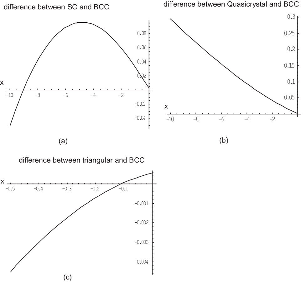
We find that when the temperature is decreased just below the transition temperature of the lattices, the lattices with a cubic term have a smaller free energy than the lattices which do not. Fig.10 shows that BCC lattice has the lowest free energy and the highest transition temperature in a range just below the transition point.
References
- (1) P. Fulde and R. A. Ferrell, Phys. Rev. 135, A550?A563 (1964).
- (2) A. I. Larkin and Yu. N. Ovchinnikov, Sov. Phys. JETP 20, 762(1965)
- (3) Ganpathy Murthy, R.Shankar, J. Phys. Condens. Matter 7, 9155 (1995).
- (4) Roberto Casalbuoni and Giuseppe Nardulli, Rev. Mod. Phys. 76, 263 (2004) and references therein.
- (5) K. Gloos, R. Modler, H. Schimanski, C. D. Bredl, C. Geibel, F. Steglich, A. I. Buzdin, N. Sato, and T. Komatsubara, Phys. Rev. Lett. 70, 501-504 (1993); R. Modler, et.al, Phys. Rev. Lett. 76, 1292-1295 (1996).
- (6) A. Bianchi,1 R. Movshovich,1 C. Capan,1 P. G. Pagliuso,2 and J. L.Sarrao1, Phys. Rev. Lett. 91, 187004 (2003).
- Martin (2005) C. Martin, C. C. Agosta, S. W. Tozer, H. A. Radovan, E. C. Palm, T. P. Murphy, and J. L. Sarrao, Phys. Rev. B 71, 020503 (2005).
- Capan (2004) C. Capan, A. Bianchi, R. Movshovich, A. D. Christianson, A. Malinowski, M. F. Hundley, A. Lacerda, P. G. Pagliuso, and J. L. Sarrao, Phys. Rev. B 70, 134513 (2004).
- (9) A. I. Buzdin, Rev. Mod. Phys. 77, 935 (2005) .
- (10) T. Mizushima, K. Machida, and M. Ichioka, Phys. Rev. Lett. 94, 060404 (2005); C.-H. Pao, Shin-Tza Wu, S.-K. Yip, cond-mat/0506437s; D.T.Son, M.A.Stephanov, cond-mat/0507586; Daniel E. Sheehy, Leo Radzihovsky, cond-mat/0508430.
- (11) N. Yoshida and S. K. Yip, cond-mat/0703205.
- P. M. Chaikin (1995) P. M. Chaikin and T. C. Lubensky principles of condensed matter physics( Cambridge university press,1995.)
- (13) S. A. Brazovskii, Phase transition of an isotropic system to a nonuniform state, JETP 41, 85 (1975).
- (14) Jinwu Ye, cond-mat/0603269.
- (15) M. Houzet and A. Buzdin, Europhys. Lett. 50, 375 (2000).
- (16) M. Houzet, A. Buzdin, L. Bulaevskii, and M. Maley, Phys. Rev. Lett. 88, 227001 (2002).
- (17) Kun Yang and A. H. MacDonald,Phys. Rev. B 70, 094512 (2004)
- (18) Jinwu Ye, cond-mat/0310512
- (19) Jinwu Ye, unpublished.
- (20) Jinwu Ye and Longhua Jiang, cond-mat/0606639, to be published in Phys. Rev. Lett.