Curve shortening and the topology
of closed geodesics on surfaces

If $M$ is a surface with a Riemannian metric $g$ then closed geodesics on $(M,g)$ are critical points of the length functional $L(\gamma)=\int|\gamma^{\prime}(x)|dx$ defined on the space of unparametrized $C^{2}$ immersed curves with orientation, i.e. we consider closed geodesics to be elements of the space

Here $\mathrm{Imm}(S^{1},M)=\{\gamma\in C^{2}(S^{1},M)\mid\gamma^{\prime}(\xi)\neq 0\text{ for all $\xi\in S^{1}$}\}$ and $\mathrm{Diff}_{+}(S^{1})$ is the group of $C^{2}$ orientation preserving diffeomorphisms of $S^{1}={\mathbb{R}}/{\mathbb{Z}}$. (We will abuse notation freely, and use the same symbol $\gamma$ to denote both a convenient parametrization in $C^{2}(S^{1};M)$, and its corresponding equivalence class in $\Omega$.)

The natural gradient flow of the length functional is given by curve shortening, i.e. by the evolution equation

In 1905 Poincaré [33] pointed out that geodesics on surfaces are immersed curves without self-tangencies. Similarly, different geodesics cannot be tangent – all their intersections must be transverse. This allows one to classify closed geodesics by their number of self-intersections, or their “flat knot type,” and to ask how many closed geodesics of a given “type” exist on a given surface $(M,g)$. Our main observation here is that the curve shortening flow (1) is the right tool to deal with this question.

We formalize these notions in the following definitions (which are a special case of the theory described by Arnol’d in [13].)

Flat knots A curve $\gamma\in\Omega$ is a flat knot if it has no self-tangencies. Two flat knots $\alpha$ and $\beta$ are equivalent if there is a continuous family of flat knots $\{\gamma_{\theta}\mid 0\leq\theta\leq 1\}$ with $\gamma_{0}=\alpha$ and $\gamma_{1}=\beta$.

Relative flat knots For a given finite collection of immersed curves,

we define a flat knot relative to $\Gamma$ to be any $\gamma\in\Omega$ which has no self-tangencies, and which is transverse to all $\gamma_{j}\in\Gamma$. Two flat knots relative to $\Gamma$ are equivalent if one can be deformed into the other through a family of flat knots relative to $\Gamma$.

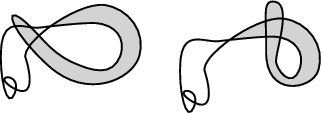
Clearly equivalent flat knots have the same number of self-intersections since this number cannot change during a deformation through flat knots. The converse is not true: Flat knots with the same number of self-intersections need not be equivalent. See Figure 1. Similarly, two equivalent flat knots relative to $\Gamma=\{\gamma_{1},\dots,\gamma_{N}\}$ have the same number of self-intersections, and the same number of intersections with each $\gamma_{j}$.

In this terminology any closed geodesic on a surface is a flat knot, and for given closed geodesics $\{\gamma_{1},\dots,\gamma_{N}\}$ any other closed geodesic is a flat knot relative to $\{\gamma_{1},\dots,\gamma_{N}\}$.

One can now ask the following question: Given a Riemannian metric $g$ on a surface $M$, closed geodesics $\gamma_{1},\dots,\gamma_{N}$ for this metric, and a flat knot $\alpha$ relative to $\Gamma=\{\gamma_{1},\dots,\gamma_{N}\}$, how many closed geodesics on $(M,g)$ define flat knots relative to $\Gamma$ which are equivalent to $\alpha$? In this paper we will use curve shortening to obtain a lower bound for the number of such closed geodesics which only depends on the relative flat knot $\alpha$, and the linearization of the geodesic flow on $(TM,g)$ along the given closed geodesics $\gamma_{j}$.

Our strategy for estimating the number of closed geodesics equivalent to a given relative flat knot $\alpha$ is to consider the set ${\mathcal{B}}_{\alpha}\subset\Omega$ of all flat knots relative to $\Gamma$ which are equivalent to $\alpha$. This set turns out to be almost an isolating block in the sense of Conley [17] for the curve shortening flow. We then define a Conley index $h({\mathcal{B}}_{\alpha})$ of ${\mathcal{B}}_{\alpha}$ and use standard variational arguments to conclude that nontriviality of the Conley index of a relative flat knot implies existence of a critical point for curve shortening in ${\mathcal{B}}_{\alpha}$.

To do all this we have to overcome a few obstacles.

First, the curve shortening flow is not a globally defined flow or even semiflow. Given any initial curve $\gamma(0)\in\Omega$ a solution $\gamma:[0,T)\to\Omega$ to curve shortening exists for a short time $T=T(\gamma_{0})>0$, but this solution often becomes singular in finite time. What helps us overcome this problem is that the set of initial curves $\gamma(0)\in{\mathcal{B}}_{\alpha}$ which are close to forming a singularity is attracting. Indeed, the existing analysis of the singularities of curve shortening in [24], [7], [25], [26], [32] shows that such singularities essentially only form when “a small loop in the curve $\gamma(t)$ contracts as $t\nearrow T(\gamma(0))$.” A calculation involving the Gauss-Bonnet theorem shows that once a curve has a sufficiently small loop the area enclosed by this loop must decrease under curve shortening. This observation allows us to include the set of curves $\gamma\in{\mathcal{B}}_{\alpha}$ with a small loop in the exit set of the curve shortening flow. With this modification we can proceed as if the curve shortening flow were defined globally.

Second, ${\mathcal{B}}_{\alpha}$ is not a closed subset of $\Omega$ and its boundary may contain closed geodesics, i.e. critical points of curve shortening: such critical points are always multiple covers of shorter geodesics. To deal with this, one must analyze the curve shortening flow near multiple covers of closed geodesics. It turns out that all relevant information to our problem is contained in Poincaré’s rotation number of a closed geodesic. In the end our Conley index $h({\mathcal{B}}_{\alpha})$ depends not only on the relative flat knot class ${\mathcal{B}}_{\alpha}$, but also on the rotation numbers of the given closed geodesics $\{\gamma_{1},\dots,\gamma_{N}\}$.

Finally, the space ${\mathcal{B}}_{\alpha}$ on which curve shortening is defined is not locally compact so that Conley’s theory does not apply without modification. It turns out that the regularizing effect of curve shortening provides an adequate substitute for the absence of local compactness of ${\mathcal{B}}_{\alpha}$.

After resolving these issues one merely has to compute the Conley index of any relative flat knot type to estimate the number of closed geodesics of that type. To describe the results we need to discuss satellites and Poincaré’s rotation number.

Poincaré [33] observed that a $(p,q)$-satellite of a simple closed curve $\alpha$ has $2p$ intersections with $\alpha$ and $p(q-1)$ self-intersections. See also Lemma 2.1.

Poincar \́hskip-6.5pte’s rotation number Let $\gamma(s)$ be an arc-length parametrization of a closed geodesic of length $L>0$ on $(M,g)$. Thus $\gamma(s+L)\equiv\gamma(s)$, and $T=\gamma^{\prime}(s)$ satisfies $\nabla_{T}T=0$. Jacobi fields are solutions of the second order ODE

where $K:M\to{\mathbb{R}}$ is the Gaussian curvature of $(M,g)$.

Let $y:{\mathbb{R}}\to{\mathbb{R}}$ be any Jacobi field, and label the zeroes of $y$ in increasing order

with $(-1)^{n}y^{\prime}(s_{n})>0$. Using the Sturm oscillation theorems one can then show that the limit

exists and is independent of the chosen Jacobi field $y$. We call this number the Poincaré rotation number of the geodesic $\gamma$. If there is a Jacobi field with only finitely many zeroes then the oscillation theorems again imply that $y(s)$ has either one or no zeroes $s\in{\mathbb{R}}$. In this case we say the rotation number is infinite.

For an alternative definition we observe that if $y(s)$ is a Jacobi field then $y(s)$ and $y^{\prime}(s)$ cannot vanish simultaneously. Thus one can consider

Again it turns out that this limit exists and is independent of the particular choice of Jacobi field $y$. Moreover one has

We call $\rho$ the inverse rotation number of $\gamma$. See [27] where the much more complicated case of quasi-periodic potentials is treated. The inverse rotation number $\rho$ is analogous to the “amount of rotation” of a periodic orbit of a twist map introduced by Mather in [30].

Allowable metrics for a given relative flat knot and the nonresonance condition Let $\Gamma=\{\gamma_{1},\dots,\gamma_{N}\}\subset\Omega$ be a collection of curves with no mutual or self-tangencies, and denote by ${\mathcal{M}}_{\Gamma}$ the space of $C^{2,\mu}$ Riemannian metrics $g$ on $M$ for which the $\gamma_{i}\in\Gamma$ are geodesics (thus the metric has continuous derivatives of second order which are Hölder continuous of some exponent $\mu\in(0,1)$). When written out in coordinates one sees that this condition is quadratic in the components $g_{ij}$ and $\partial_{i}g_{jk}$ of the metric and its derivatives. Thus ${\mathcal{M}}_{\Gamma}$ is a closed subspace of the space of $C^{2,\mu}$ metrics on ${\mathcal{M}}$.

If $\alpha\in\Omega$ is a flat knot rel $\Gamma$ then it may happen that $\alpha$ is a $(p_{1},q_{1})$ satellite of, say, $\gamma_{1}$. In this case the rotation number of $\gamma_{1}$ will affect the number of closed geodesics of flat knot type $\alpha$ rel $\Gamma$. To see this, consider a family of metrics $\{g_{\lambda}\mid\lambda\in{\mathbb{R}}\}\subset{\mathcal{M}}_{\gamma}$ for which the inverse rotation number $\rho(\gamma;g_{\lambda})$ is less than $p_{1}/q_{1}$ for negative $\lambda$ and more than $p_{1}/q_{1}$ for positive $\lambda$. Then, as $\lambda$ increases from negative to positive, a bifurcation takes place in which generically two $(p_{1},q_{1})$ satellites of $\gamma_{1}$ are created. These bifurcations appear as resonances in the Birkhoff normal form of the geodesic flow on the unit tangent bundle near the lift of $\gamma$. This is described by Poincaré in [33, §6, p. 261]. See also [14, Appendix 7D,F].

In studying the closed geodesics of flat knot type $\alpha$ rel $\Gamma$ we will therefore exclude those metrics for which a bifurcation can take place. To be precise, given $\alpha$ we order the $\gamma_{i}$ so that $\alpha$ is a $(p_{i},q_{i})$ satellite of $\gamma_{i}$, if $1\leq i\leq m$, but not a satellite of $\gamma_{i}$ for $m<i\leq N$. We then impose the nonresonance condition

The metrics $g\in{\mathcal{M}}_{\Gamma}$ which satisfy this condition can be separated into $2^{m}$ distinct classes. For any subset $I\subset\{1,\dots,m\}$ we define ${\mathcal{M}}_{\Gamma}(\alpha;I)$ to be the set of all metrics $g\in{\mathcal{M}}_{\Gamma}$ such that the inverse rotation numbers $\rho(\gamma_{1})$, …, $\rho(\gamma_{m})$ satisfy

For each $I\subset\{1,\dots,m\}$ we define in Section 6 a Conley index $h^{I}$. This is done by choosing a metric $g\in{\mathcal{M}}_{\Gamma}(\alpha;I)$, suitably modifying the set ${\mathcal{B}}_{\alpha}\subset\Omega$ and its exit set for the curve shortening flow, according to the choice of $I\subset\{1,\dots,m\}$ and then finally setting $h^{I}$ equal to the homotopy type of the modified ${\mathcal{B}}_{\alpha}$ with its exit set collapsed to a point. Thus the index we define is the homotopy type of a topological space with a distinguished point. We show that the resulting index $h^{I}$ does not depend on the choice of metric $g\in{\mathcal{M}}(\alpha;I)$, and also that the index $h^{I}$ does not change if one replaces $\alpha$ by an equivalent flat knot rel $\Gamma$.

Using rather standard variational methods we then show in §7:

Using more standard variational arguments one could then improve on this and show that there are at least $n-1$ closed geodesics of type $\alpha$ rel $\Gamma$, where $n$ is the Lyusternik-Schnirelman category of the pointed topological space $h^{I}$. We do not use this result here and omit the proof.

Computation of the index $h^{I}$ for an arbitrary flat knot $\alpha$ rel $\Gamma$ may be difficult. It is simplified somewhat by the independence of $h^{I}$ from the metric $g\in{\mathcal{M}}_{\Gamma}(\alpha;I)$. In addition we have a long exact sequence which relates the homologies of the different indices one gets by varying $I$.

This immediately implies

One may regard this as a global bifurcation theorem. If for some choice of rotation numbers $I$ and some choice of metric $g\in{\mathcal{M}}_{\Gamma}(\alpha;I)$ there are no closed geodesics of type $\alpha$ rel $\Gamma$, then the index $h^{I}$ is trivial. By increasing one or more of the rotation numbers (i.e. increasing $I$ to $J$), or by decreasing some of the rotation numbers (i.e. decreasing $I$ to $J$) the index $h^{I}$ becomes nontrivial, and a closed geodesic of type $\alpha$ rel $\Gamma$ must exist for any metric $g\in{\mathcal{M}}_{\Gamma}(\alpha;J)$.

When applied to the case where $M=S^{2}$ and $\Gamma$ consists of one simple closed curve $\gamma$ this gives us the following result.

Acknowledgements. The work in this paper was inspired by a question of Hofer (Oberwollfach, 1993) who asked me if one could apply the Floer homology construction to curve shortening, and which results could be obtained in this way. This turned out to be a very fruitful question, even though in the end curve shortening appears to be sufficiently well behaved to use the Conley index instead of Floer’s approach.

The paper was finished during my sabattical at the University of Leiden. It is a pleasure to thank Rob van der Vorst, Bert Peletier and Sjoerd Verduyn Lunel for their hospitality.

The space of immersed curves The space of immersed curves $\Omega=\mathrm{Imm}(S^{1}$, $M)/\mathrm{Diff}_{+}\left(S^{1}\right)$ is locally homeomorphic to $C^{2}({\mathbb{R}}/{\mathbb{Z}})$. The homeomorphisms are given by the following charts. Let $\gamma\in\Omega$ be a given immersed curve. Choose a $C^{2}$ parametrization $\gamma:{\mathbb{R}}/{\mathbb{Z}}\to M$ of this curve and extend it to a $C^{2}$ local diffeomorphism $\sigma:({\mathbb{R}}/{\mathbb{Z}})\times(-r,r)\to M$ for some $r>0$. Then for any $C^{1}$ small function $u\in C^{2}({\mathbb{R}}/{\mathbb{Z}})$ the curve

is an immersed $C^{2}$ curve. Let ${\mathcal{U}}_{r}=\{u\in C^{2}({\mathbb{R}}/{\mathbb{Z}}):|u(x)|<r\}$. For sufficiently small $r>0$ the map $\Phi:u\in{\mathcal{U}}_{r}\mapsto\gamma_{u}\in\Omega$ is a homeomorphism of ${\mathcal{U}}_{r}$ onto a small neighborhood $\Phi({\mathcal{U}}_{r})$ of $\gamma$. The open sets $\Phi({\mathcal{U}}_{r})$ which one gets by varying the curve $\gamma$ cover $\Omega$, and hence $\Omega$ is a topological Banach manifold with model $C^{2}({\mathbb{R}}/{\mathbb{Z}})$.

A natural choice for the local diffeomorphism $\sigma$ would be

where $\mathbf{N}$ is a unit normal vector field for the curve $\gamma$. We avoid this choice of $\sigma$ since it uses too many derivatives. For $\sigma$ to be $C^{2}$ one would want the normal to be $C^{2}$, so the curve would have to be $C^{3}$; one would also want the exponential map to be $C^{2}$, which requires the Christoffel symbols to have two derivatives, and so the metric $g$ would have to be $C^{3}$.

For future reference we observe that if the curve $\gamma$ is $C^{2,\mu}$ then one can also choose the diffeomorphism $\sigma$ to be $C^{2,\mu}$.

Covers For any $\gamma\in\Omega$ and any nonzero integer $q$ we define $q\cdot\gamma$ to be the $q$-fold cover of $\gamma$, i.e. the curve with parametrization

where $\gamma:{\mathbb{R}}/{\mathbb{Z}}\to M$ is a parametrization of $\gamma$. Thus $(-1)\cdot\gamma$ is the curve $\gamma$ with its orientation reversed.

A curve $\gamma\in\Omega$ will be called primitive if it is not a multiple cover of some other curve, i.e. if there are no $q\geq 2$ and $\gamma_{0}\in\Omega$ with $\gamma=q\cdot\gamma_{0}$.

Flat knots Let $\gamma_{1}$, $\dots$, $\gamma_{N}$ be a collection of primitive immersed curves in $M$. Define

Then $\Delta$ and $\Delta(\gamma_{1},\dots,\gamma_{N})$ are closed subsets of $\Omega$, and their complements $\Omega\setminus\Delta$ and $\Omega\setminus\Delta(\gamma_{1},\dots,\gamma_{N})$ consist of flat knots, and flat knots relative to $(\gamma_{1},\dots,\gamma_{N})$, respectively. Two such flat knots are equivalent if and only if they lie in the same component of $\Omega\setminus\Delta$ or $\Omega\setminus\Delta(\gamma_{1},\dots,\gamma_{N})$.

Flat knots as knots in the projective tangent bundle Let ${\mathbb{P}}TM$ be the projective tangent bundle of $M$, i.e. ${\mathbb{P}}TM$ is the bundle obtained from the unit tangent bundle

by identification of all antipodal vectors $(x,v)$ and $(x,-v)$. The projective tangent bundle is a contact manifold. If we denote the bundle projection by $\pi:{\mathbb{P}}TM\to M$, then the contact plane $L_{(x,\pm v)}\subset T({\mathbb{P}}TM)$ at a point $(x,\pm v)\in{\mathbb{P}}TM$ consists of those vectors $\xi\in T({\mathbb{P}}TM)$ for which $d\pi(\xi)$ is a multiple of $v$. Each contact plane $L_{(x,\pm v)}$ contains a nonzero vector $\vartheta$ with $d\pi(\vartheta)=0$ ($\vartheta$ corresponds to infinitesimal rotation of the unit vector $\pm v$ in the tangent space $T_{x}M$, while the base point $x$ remains fixed).

Any $\gamma\in\Omega$ defines a $C^{1}$ immersed curve ${\hat{\gamma}}$ in the projective tangent bundle ${\mathbb{P}}TM$ with parametrization ${\hat{\gamma}}(s)=(\gamma(s),\pm\gamma^{\prime}(s))$, where $\gamma(s)$ is an arc length parametrization of $\gamma$. We call ${\hat{\gamma}}$ the lift of $\gamma$.

An immersed curve $\tilde{\gamma}$ in ${\mathbb{P}}TM$ is the lift of some $\gamma\in\Omega$ if and only if $\tilde{\gamma}$ is everywhere tangent to the contact planes, and nowhere tangent to the special direction $\vartheta$ in the contact planes.

Self-tangencies of $\gamma\in\Omega$ correspond to self-intersections of its lift $\hat{\gamma}\subset{\mathbb{P}}TM$. Thus an immersed curve $\gamma\in\Omega$ is a flat knot exactly when its lift $\hat{\gamma}$ is a knot in the three manifold ${\mathbb{P}}TM$. If two curves $\gamma_{1},\gamma_{2}\in\Omega$ define equivalent flat knots then one can be deformed into the other through flat knots. By lifting the deformation we see that $\hat{\gamma}_{1}$ and $\hat{\gamma}_{2}$ are equivalent knots in ${\mathbb{P}}TM$.

Intersections If $\alpha\in\Omega\setminus\Delta(\gamma_{1}$, $\dots$, $\gamma_{n})$ then $\alpha$ is transverse to each of the $\gamma_{i}$. Hence the number of intersections in $\alpha\cap\gamma_{i}$ is well defined. This only depends on the flat knot type of $\alpha$ relative to $\gamma_{1}$, $\dots$, $\gamma_{n}$.

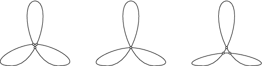
If $\alpha\in\Omega\setminus\Delta$ then $\alpha$ only has transverse self-intersections, so their number is well defined by $\#\alpha\cap\alpha=\#\{0\leq x<x^{\prime}<1\mid\alpha(x)=\alpha(x^{\prime})\}$. From a drawing of $\alpha$ they are easily counted. An $\alpha\in\Omega\setminus\Delta$ can only have double points, triple points, etc. (see Figure 2). If $\alpha$ only has double points (a generic property) then their number is the number of self-intersections. Otherwise one must count the number of geometric self-intersections where a $k$-tuple point counts for $\binom{k}{2}$ self-intersections. Again this number only depends on the flat knot type of $\alpha\in{\Omega\setminus\Delta}$.

Nontransverse crossings of curves If $\gamma_{1},\gamma_{2}\in\Omega$ are not necessarily transverse then we define the number of crossings of $\gamma_{1}$ and $\gamma_{2}$ to be

where the supremum is taken over all pairs of open neighborhoods ${\mathcal{U}}_{i}\subset\Omega$ of $\gamma_{i}$. Thus $\mathrm{Cross}(\gamma_{1},\gamma_{2})$ is the smallest number of intersections $\gamma_{1}$ and $\gamma_{2}$ can have if one perturbs them slightly to become transverse.

The number of self-crossings $\mathrm{Cross}(\gamma,\gamma)$ is defined in a similar way.

Clearly $\mathrm{Cross}(\gamma_{1},\gamma_{2})$ is a lower semicontinuous function on $\Omega\times\Omega$.

Satellites We first describe the local model of a satellite of a primitive flat knot $\gamma\in\Omega\setminus\Delta$ and then transplant the local model to primitive flat knots on any surface.

Let $q\geq 1$ be an integer, and let $u\in C^{2}({\mathbb{R}}/q{\mathbb{Z}})$ be a function for which

and

Consider the curve $\alpha_{u}$ in the cylinder $\Gamma=({\mathbb{R}}/{\mathbb{Z}})\times{\mathbb{R}}$, parametrized by

The conditions (10) and (11) imply that $\alpha_{u}$ is a flat knot relative to $\alpha_{0}$, where $\alpha_{0}=({\mathbb{R}}/{\mathbb{Z}})\times\{0\}$ is the zero section (i.e., the curve corresponding to $u(x)\equiv 0$).

Now consider a primitive flat knot $\gamma\in\Omega\setminus\Delta$. Denote by $\gamma:{\mathbb{R}}/{\mathbb{Z}}\to M$ any parametrization, and choose a local diffeomorphism $\sigma:{\mathbb{R}}/{\mathbb{Z}}\times(-r,r)\to M$ with $\gamma(x)=\sigma(x,0)$. As in §2 we then identify any curve $\gamma_{u}$ which is $C^{1}$ close to $\gamma$ with a function $u\in C^{2}({\mathbb{R}}/{\mathbb{Z}})$ via (6).

If $u\in C^{2}({\mathbb{R}}/q{\mathbb{Z}})$ then the curve defined by

is a flat knot relative to $\gamma$. For given $u\in C^{2}({\mathbb{R}}/q{\mathbb{Z}})$ and small enough $\varepsilon>0$ the $\alpha_{{\varepsilon,u}}$ all define the same relative flat knot.

By definition, a curve $\alpha\in\Omega\setminus\Delta(\gamma)$ is a satellite of $\gamma\in\Omega\setminus\Delta$ if for some $u\in C^{2}({\mathbb{R}}/q{\mathbb{Z}})$ it is isotopic relative to $\gamma$ to all $\alpha_{\varepsilon,u}$ with $\varepsilon>0$ sufficiently small.

To complete this definition we should specify the orientation of the satellite $\alpha_{\varepsilon,u}$. One can give $\alpha_{\varepsilon,u}$ as defined in (13) the same orientation as its base curve $\gamma$, or the opposite orientation. We will call both curves satellites of $\gamma$. In general the satellites $\alpha_{\varepsilon,u}$ and $-\alpha_{\varepsilon,u}$ can define different flat knots relative to $\gamma$ or they can belong to the same relative flat knot class.

Example Let $\gamma$ be the equator on the standard two sphere $M=S^{2}$. Then any other great circle is a satellite of $\gamma$. Moreover, all these great circles with either orientation define the same flat knot relative to the equator. For example, if $\alpha$ is a great circle in a plane through the $x$-axis which makes an angle $\varphi\ll\pi/2$ with the $xy$-plane, then one can reverse its orientation by first rotating it through $\pi-2\varphi$ around the $x$-axis, and then rotating it through $\pi$ around the $z$-axis. Throughout this motion the curve remains transverse to the equator, so that $\alpha$ and $-\alpha$ indeed belong to the same component of $\Delta\setminus\Omega(\gamma)$. Below we will show that this example is exceptional.

As defined in the introduction, one obtains $(p,q)$ satellites by setting

Let $p\neq 0$, and let $\alpha$ be the $(p,q)$ satellite of $\gamma$ given by $u(x)=\epsilon\sin(2\pi\frac{p}{q}x)$. Then we can translate $\alpha$ along the base curve $\gamma$; i.e. we can consider the $(p,q)$ satellites $\alpha_{\tau}$ given by $u_{\tau}(x)=\epsilon\sin(2\pi\frac{p}{q}(x-\tau))$. By translating from $\tau=0$ to $\tau=\frac{q}{2p}$ one finds an isotopy from $\alpha$ to the curve $\bar{\alpha}$ given by $\bar{u}(x)=\sin(2\pi\frac{-p}{q}x)$. Hence one can turn any $(p,q)$ satellite into a $(-p,q)$ satellite, and we may therefore always assume that $p$ is nonnegative.

We will denote the set of $(p,q)$-satellites of $\gamma\in\Omega$ by ${\mathcal{B}}_{p,q}(\gamma)$, always assuming that $p\geq 0$ and $q\geq 1$.

More precisely we will let ${\mathcal{B}}^{+}_{p,q}(\gamma)$ be the set of $(p,q)$-satellites of $\gamma$ which have the same orientation as $\gamma$, and we let ${\mathcal{B}}^{-}_{p,q}(\gamma)$ be those $(p,q)$ satellites with opposite orientation. With this notation we always have

It is not a priori clear that all these classes are disjoint, but by counting the number of self-intersections of $(p,q)$ satellites one can at least see that there are infinitely many disjoint ${\mathcal{B}}_{p,q}$’s.

This was observed by Poincaré [33]. We include a proof for completeness’ sake.

Intersections of $\alpha$ and $\gamma$ are of two types. Each zero of $u(x)$ corresponds to an intersection of $\alpha$ and $\gamma$. At each self-intersection of $\gamma$ the two intersecting strands of $\gamma$ are accompanied by $2q$ strands of $\alpha$ which intersect $\gamma$ in $2q$ points. Since $u(x)$ has $2p$ zeroes and $\gamma$ has $m$ self-intersections we get $2mq+2p$ intersections of $\alpha$ and $\gamma$.

To count self-intersections one must count the intersections of the graph of $u(x)=\sin(2\pi\frac{p}{q}x)$ wrapped up on the cylinder $\Gamma=({\mathbb{R}}/{\mathbb{Z}})\times{\mathbb{R}}$, i.e. the intersections of the graphs of $u_{k}(x)=u(x-2k)$ ($k=0,1,\dots,q-1$) with $0\leq x<2\pi$. After some work one finds that these are arranged in $q-1$ horizontal rows, each of which contains $p$ intersections.

At each self-intersection of $\gamma$ two strands of $\gamma$ cross. If $\varepsilon$ is small enough then $\alpha_{\varepsilon,u}$ is locally almost parallel to $\gamma$, so that any pair of crossing strands of $\gamma$ is accompanied by a pair of $q$ nearly parallel strands of $\alpha$ which cross each other. This way we get $q^{2}$ extra self-crossings of $\alpha$ and $2q$ extra crossings of $\gamma$ with $\alpha$ per self-crossing of $\gamma$. ∎

If $\alpha\in{\mathcal{B}}_{p,q}$ has $2k$ intersections with $\gamma$ and $l$ self-intersections then

Substitute $p=k-mq$ in the first equation to get

from which one finds $q=\frac{k+l}{k+m}$. In particular, the numbers $k$, $l$ and $m$ determine $p$ and $q$. \Endproof

The proof also shows that most satellites are not $(p,q)$-satellites for any $(p,q)$. Indeed, given $\alpha\in{\mathcal{B}}_{p,q}(\gamma)$ one can modify it near one of its crossings with $\gamma$ so as to increase the number $k$ of intersections with $\gamma$ arbitrarily without changing the number of self-intersections $l$, or $m$. Unless both $l=0$ and $m=0$, then for large enough $k$ the fraction $\frac{k+l}{k+m}$ will not be an integer, so the modified curve can no longer be a $(p,q)$ satellite. If both $l=m=0$ then both $\gamma$ and its satellite $\alpha$ must be simple curves.

$(p,q)$ satellites along a simple closed curve on $S^{2}$ In this section we consider the case in which $M=S^{2}$ and $\zeta\in\Omega$ is a simple closed curve. We will show that for all $(p,q)$ except $p=q=1$ the classes ${\mathcal{B}}^{\pm}_{p,q}(\zeta)$ are different.

After applying a diffeomorphism we may assume that $M$ is the unit sphere in ${\mathbb{R}}^{3}$ and that $\zeta$ is the equator, given by $z=0$.

To study curves in $\Omega\setminus\Delta(\zeta)$ it is useful to recall that one can identify the unit tangent bundle $T^{1}(S^{2})$ of the 2-sphere with the group SO$(3,{\mathbb{R}})$. Indeed, by definition,

so that any unit tangent vector $(\vec{x},\vec{\xi})\in T^{1}(S^{2})$ determines the first two columns of an orthogonal matrix. The third column of this matrix is the cross product $\vec{x}\times\vec{\xi}$. The map

is a diffeomorphism, and from here on we will simply identify $T^{1}(S^{2})$ and SO$(3,{\mathbb{R}})$.

Let ${\mathcal{U}}\subset T^{1}(S^{2})$ be the complement of the set of tangent vectors to $\zeta$ and $-\zeta$. One can describe ${\mathcal{U}}$ very conveniently using “Euler Angles”. For the definition of these angles we refer to Figure 3. Any unit tangent vector $(\vec{x},\vec{\xi})$ defines an oriented great circle, parametrized by

Unless $(\vec{x},\vec{\xi})$ is a tangent vector of the equator $\pm\zeta$, the great circle through $(\vec{x},\vec{\xi})$ intersects the equator in two points. In one of these intersections the great circle crosses the equator from south to north. Let $\theta$ be the angle from the upward intersection to $x$, so that $X(-\theta)$ is the upward intersection point. We define $\psi$ to be the angle between the plane through the great circle $\{X(t)\mid t\in{\mathbb{R}}\}$ and the $xy$-plane (so that $0<\psi<\pi$). Finally we let $\phi$ be the angle along the equator $\zeta$ from the $x$-axis to the upward intersection point $X(-\theta)$.

If we denote the matrix corresponding to a rotation by an angle $\alpha$ around the $x$ axis by ${\rm R}_{x}(\alpha)$, etc. then the relation between the Euler angles $(\theta,\varphi,\psi)$ and the unit tangent vector $(x,\xi)$ they represent is given by

The map $(\vec{x},\vec{\xi})\mapsto(\theta,\psi,\phi)$ is a diffeomorphism between ${\mathcal{U}}$ and $({\mathbb{R}}/2\pi{\mathbb{Z}})\times(0,\pi)\times({\mathbb{R}}/2\pi{\mathbb{Z}})\cong{\mathbb{T}}^{2}\times{\mathbb{R}}$.

Given this identification we can now define two numerical invariants of flat knots $\alpha$ relative to the equator $\zeta$. By the lift of a unit speed parametrization, any flat knot $\alpha\in\Omega\setminus\Delta(\zeta)$ defines a closed curve $\hat{\alpha}:S^{1}\to{\mathcal{U}}$. The numerical invariants are then the increments of the Euler angles $\theta$ and $\phi$ along $\hat{\alpha}$, which we will denote by $\Delta\theta(\alpha)$ and $\Delta\phi(\alpha)$, respectively. Both are integral multiples of $2\pi$.

Note that the number of zeroes of $u\in C^{2}({\mathbb{R}}/2\pi{\mathbb{Z}})$ must always be even (assuming they are all simple zeroes, of course). \ProofWe project the sphere onto the cylinder $x^{2}+y^{2}=1$ and write $z$ and $\vartheta$ for the usual coordinates on this cylinder. We assume that $\alpha$ projects to the graph of $z=u(\vartheta)$ on the cylinder, and that $u$ is a 2$q\pi$ periodic function with simple zeroes only, and for which $|u(\vartheta)|+|u^{\prime}(\vartheta)|$ is uniformly small.

Let $\alpha$ have the same orientation as the equator (from west to east). We compute the Euler angles corresponding to the unit tangent vector to $\alpha$ at the point which projects to $(\vartheta_{0},u(\vartheta_{0}))$ on the cylinder. In Figure 4 we have sketched the great circle which passes through $(\vartheta_{0},u(\vartheta_{0}))$ with slope $u^{\prime}(\vartheta_{0})$ as it appears in($\vartheta$, $z$) coordinates on the cylinder. Since great circles are intersections of planes through the origin with the sphere, they project to intersections of such planes with the cylinder, and are therefore graphs of $z=\psi\sin(\vartheta-\phi)$.

From Figure 4 one finds

so that

From (17) we see that $\theta+\phi$ increases by $2q\pi$ along the curve $\alpha$. To compute $\Delta\phi$ we use (18) and count the number of times the curve $u^{\prime}(\vartheta_{0})+iu(\vartheta_{0})$ in the complex plane crosses the positive real axis. Every such crossing corresponds to a zero of $u$ with positive derivative, and hence there are $\frac{2p}{2}=p$ of them. We conclude that $\Delta\theta=p\times 2\pi$, as claimed.

Similar arguments also allow one to find $\Delta\phi$ and $\Delta\theta$ if one gives $\alpha$ the orientation opposite to that of the equator. \Endproof

We have observed that ${\mathcal{B}}_{1,1}^{+}(\zeta)$ and ${\mathcal{B}}_{1,1}^{-}(\zeta)$ coincide. If $p/q$ is any fraction in lowest terms then ${\mathcal{B}}_{p,q}^{+}(\zeta)={\mathcal{B}}_{p,q}^{-}(\zeta)$ combined with (16a) implies $\Delta\theta=0$, and hence $p=q$. Since $\mathrm{gcd}(p,q)=1$ we conclude

The gradient flow of the length functional Let $g$ be a $C^{2,\mu}$ metric on the surface $M$. Then for any $C^{1}$ initial immersed curve $\gamma_{0}$ a maximal classical solution to curve shortening exists on a time interval $0\leq t<T(\gamma_{0})$. We denote this solution by $\{\gamma_{t}:0\leq t<T(\gamma_{0})\}$. The solution depends continuously on the initial data $\gamma_{0}\in\Omega$, so that curve shortening generates a continuous local semiflow

One can show that if $T(\gamma_{0})<\infty$ then the geodesic curvature $\kappa_{\gamma_{t}}$ of $\gamma_{t}$ “blows-up” as $t\nearrow T(\gamma_{0})$, i.e.

Since the geodesic curvature itself satisfies a parabolic equation