The Stueckelberg Extension and
Milli Weak and Milli Charged Dark Matter
Abstract
A overview is given of the recent developments in the Stueckelberg extensions of the Standard Model and of MSSM where all the Standard Model particles are neutral under the , but an axion which is absorbed is charged under both and and acts as the connector field coupling the Standard Model sector with the Stueckelberg sector. Coupled with the usual Higgs mechanism that breaks the gauge symmetry, this scenario produces mixings in the neutral gauge boson sector generating an extra boson. The couplings of the extra to the Standard Model particles are milli weak but its couplings to the hidden sector matter, defined as matter that couples only to the gauge field of , can be of normal electro-weak strength. It is shown that such extensions, aside from the possibility of leading to a sharp resonance, lead to two new types of dark matter: milli weak (or extra weak) and milli charged. An analysis of the relic density shows that the WMAP-3 constraints can be satisfied for either of these scenarios. The types of models discussed could arise as possible field point limit of certain Type IIB orientifold string models.
Keywords:
U(1) extension, Stueckelberg, milli weak, milli-charged, dark matterClassification:
14.70.Pw, 95.34. +d, 12.60.Cn1 Introduction
Through a Stueckelberg mechanism an Abelian gauge boson develops mass without the benefit of a Higgs mechanism (For the early history of the Stueckelberg mechanism see, Stueckelberg 1938; Ogievetskii and Polubarinov 1962; Chodos and Cooper 1971; Kalb and Ramond 1974). Thus consider the Lagrangian
| (1) |
which is gauge invariant under the transformations . With the gauge fixing term , the total Lagrangian reads
| (2) |
where we have added also an interaction term which contains the coupling of with fermions via a conserved current with . Here the fields and are decoupled and renormalizability and unitarity are manifest. Mass growth by the Stueckelberg mechanism occur quite naturally D brane constructions where one encounters the group for a stack of D branes which is then broken to its subgroup via Stueckelberg couplings. Thus, for example, one has
| (3) |
2 The Stueckelberg extension of SM
The Stueckelberg extension can be used for the extensions of the Standard Model Kors and Nath 2004a and of MSSM Kors and Nath 2004b; Kors and Nath 2005; Kors and Nath 2004c. We begin by discussing the Stueckelberg extension of the Standard Model Kors and Nath 2004a where we write the Lagrangian so that , where
| (4) |
It is easily checked that the above Lagrangian is invariant under the following transformations : and . The two Abelian gauge bosons can be decoupled from by the addition of gauge fixing terms as before. Additionally, of course, one has to add the standard gauge fixing terms for the SM gauge bosons to decouple from the Higgs.
We look now at the physical content of the theory. In the vector boson sector in the basis , the mass matrix for the vector bosons takes the form
| (5) |
where and are the and gauge coupling constants, and are normalized so that . It is easily checked that which implies that one of the eigenvalues is zero, whose eigenvector we identify with the photon. The remaining two eigenvalues are non-vanishing and correspond to the and bosons. The symmetric matrix can be diagonalized by an orthogonal transformation, , with so that the eigenvalues are given by the set : . One can solve for explicitly and we use the parametrization
where The third angle is given by . This allows one to choose and as two independent parameters to characterize physics beyond SM. There is also a modification of the expression of the electric charge in terms of SM parameters. Thus if we write the EM interaction in the form the expression for is given by
| (6) |
The LEP and Tevatron data puts stringent bounds on . One finds Feldman et al. 2006a; Feldman et al. 2006b that it is constrained by in most of the parameter space. In the absence of a hidden sector, i.e., the matter sector that couples only to , the can decay only into visible sector quarks and leptons, and its decay width is governed by and hence the is very sharp, with a width that lies in the range of of maximally several hundred MeV compared to several GeV that one expects for a arising from a GUT group (a narrow can also arise in other models, see e.g., Chang et al. 2006; Battaglia et al. 2005; Burdman et al. 2006; Ferroglia et al. 2006; Davoudiasl et al. 2000). However, even a very sharp is discernible at the Tevatron and at the LHC using the dilepton signal. On the other hand if a hidden sector exists with normal size gauge coupling to the then can decay into the hidden sector particles and will have a width in the several GeV range. In this case the branching ratio of to will be very small Cheung and Yuan 2007; Feldman et al. 2007a and the dilepton signal will not be detectable. We will return to this issue in the context of milli charged dark matter.
3 Stueckelberg extension of the minimal supersymmetric standard model
To obtain the supersymmetric Steuckelberg extension Kors and Nath 2004b; Kors and Nath 2004c; Kors and Nath 2005 we consider the Stueckelberg chiral multiplet along with the vector superfield multiplets for the denoted by and for the denoted by . The Stueckelberg addition to the SM Lagrangian is then given by
| (7) |
Under and the supersymmetrized gauge transformations are then given by: and . Expanding the fields in the component form, in the Wess-Zumino gauge, we have for a vector superfield, denoted here by ,
| (8) |
The superfield in component notation is given by
| (9) | |||||
We note that the superfield S contains the scalar and the axionic pseudo-scalar . In component form then has the form
| (10) | |||||
To the above we can add the gauge fields of the Standard Model which give
The gauge fields can be coupled to the chiral superfields of matter in the usual way
Here , and where is the hypercharge so that . We assume that the SM matter fields do not carry any charge under the hidden gauge group, i.e. . The Stueckelberg extensions of the type we have discussed could have origin in Type IIB orientifold models Ghilencea et al. 2002; Ghilencea 2003; Ibanez et al. 2001; Antoniadis et al. 2003; Blumenhagen et al. 2002 and several recent works appear to recover in its low energy limit the type of models discussed here Anastasopoulos et al. 2006a; Anastasopoulos et al. 2006b; Coriano’ et al. 2006; Coriano et al. 2007a; Coriano et al. 2007b; Anastasopoulos 2007; Coriano and Irges 2006.
3.1 Milli weak dark matter in extension
We note that the Stueckelberg extension brings in two more Majorana spinors which we can construct out of the Weyl spinors as follows . This enlarges the neutralino mass matrix from being as is the case in MSSM to a mass matrix in the Stueckelberg extension. The enlarged neutralino mass matrix reads
| (11) |
Here the matrix on the lower right hand corner is the usual neutralino mass matrix of MSSM, while the matrix in the top left hand corner is due the Stueckelberg extension. The term is the soft breaking term which is added by hand. The zero entry in the upper left hand corner arises due to the Weyl fermions not acquiring soft masses. The matrix gives rise to six Majorana mass eigenstates which may be labeled as follows , where the two additional Majorana eigenstates are due to the Stueckelberg extension. We label these two and to leading order in their masses are given by
| (12) |
where . If the mass of is less than the mass of other sparticles, then will be a candidate for dark matter with R parity conservation. These are what one may call XWIMPS (mWIMPS) for extra (milli) weakly interacting massive particles. Here the satisfaction of relic density requires coannihilation and one has to consider processes of the type , where etc denote the Standard Model final states. In this case we can write the effective cross section as followsFeldman et al. 2007b
| (13) |
Here is the degeneracy for the corresponding particle, where is the freeze-out temperature, and is the mass gap. For the case of XWIMPS one has . Now it is easily seen that when the mass gap between and is large and , then is much smaller than the typical WIMP cross-section and in this case one does not have an efficient annihilation of the XWIMPS. On the other hand if the mass gap between the XWIMP and WIMP is small then coannihilation of XWIMPs is efficient. In this case and one has . The above result is valid more generally with many channels participating in the coannihilations, as can be seen by defining an effective Q given by where . Thus, satisfaction of the relic density constraints arise quite easily for the XWIMPS. A detailed analysis of the relic density of XWIMPS was carried out in Feldman et al. 2007b and it was found that the WMAP-3 constraintSpergel et al. 2006 can be satisfied by XWIMPS.
4 Stueckelberg mechanism with kinetic mixing
We discuss now the Stueckelberg extension with kinetic mixing Feldman et al. 2007a for which we take the Lagrangian to be of the form where
| (14) |
In this case the kinetic mixing matrix,in the basis is,
| (15) |
A simultaneous diagonalization of the kinetic energy and of the mass matrix can be obtained by a transformation , which is a combination of a transformation () and an orthogonal transformation (). This allows one to work in the diagonal basis, denoted by , through the transformation , where the matrix which diagonalizes the kinetic terms has the form
| (16) |
The diagonalization also leads to the following relation for the electronic charge
| (17) |
Thus is related to by . In the absence of a hidden sector, there is only one parameter that enters in the analysis of electroweak fits. This effective parameter is given by . Thus one can satisfy the LEP and the Tevatron electro-weak data with but and could be individually larger.

4.1 How milli charge is generated in Stueckelberg extension
To exhibit the phenomenon of generation of milli-charge in the Stueckelberg model we consider two gauge fields corresponding to the gauge groups and . We choose the following Lagrangian where
| (18) |
Here is the current arising from the physical sector including quarks, leptons, and the Higgs fields and is the current arising from the hidden sector. As indicated in the discussion preceding Eq.(16), the mass matrix can be diagonalized by the transformation which for this example is parameterized as follows
| (19) |
where is determined by the diagonalization constraint so that
| (20) |
The diagonalization yields one massless mode and one massive mode . In this case the interaction Lagrangian in the diagonal basis assumes the formFeldman et al. 2007a
| (21) | |||||
The interesting phenomenon to note here is that the photon field couples with the hidden sector current only due to mass mixing, i.e., only due to . Thus the origin of milli charge is due to the Stueckelberg mass mixing both in the presence or absence of kinetic mixing. This phenomenon persists when one considers where the gauge group is broken by the conventional Higgs mechanism and in addition one has the Stueckelberg mechanism generating a mass mixing between the and . The above phenomenon is to be contrasted with the kinetic mixing model Holdom 1986 where one has two massless modes (the photon and the paraphoton) and the photon can couple with the hidden sector because of kinetic mixing generating milli charge couplings. [An analysis with kinetic mixing and mass mixings of a different type than discussed here is also considered in Holdom 1991].
4.2 Milli charge dark matter
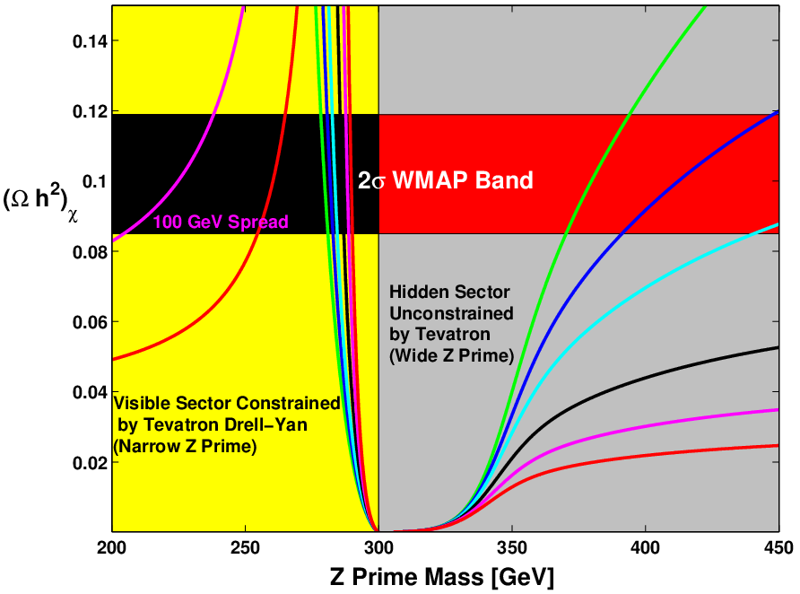
The hidden sector particles are typically natural candidates for dark matter. The main issue concerns their ability to annihilate in sufficient amounts to satisfy the current relic density constraints. Now the milli charged particles could decay in sufficient amounts by decaying via the to the Standard Model particles if their masses are . An explicit analysis of this possibility is carried out in Cheung and Yuan 2007 where a pair of Dirac fermions were put in the hidden sector which couple with strength with the Stueckelberg field . In this case it was shown that the relic density constraints consistent with the WMAP-3 data can be satisfied. Further, with inclusion of proper thermal averaging of the quantity over the resonant [using techniques discussed in Nath and Arnowitt 1993; Baer and Brhlik 1996; Gondolo and Gelmini 1991; Griest and Seckel 1991; Arnowitt and Nath 1993] which enters in the relic density analysis, one finds that the WMAP-3 relic density constraints can also be satisfied over a broad range when the masses of the milli charged hidden sector particles lie above , with and without kinetic mixingFeldman et al. 2007a. This phenomenon comes about because of the thermal averaging effect. On the branch where the milli charged particles have masses lying above the relic density constraints can be satisfied and still produce a dilepton signal which may be observable at the LHC. Feldman et al. 2007a. Satisfaction of the relic density constraints consistent with WMAP-3 and illustration of the strong dilepton signal are seen in Figs.(1,2)[taken from Feldman et al. 2007a]. The experimental constraints on milli charged particles have been discussed in a number of papers in the literature mostly in the context of kinetic mixing models, Goldberg and Hall 1986; Golowich and Robinett 1987; Mohapatra and Rothstein 1990; Davidson and Peskin 1994; Foot et al. 1990; Caldwell et al. 1988; Dobroliubov and Ignatiev 1990; Davidson et al. 2000; Perl et al. 2001; Prinz et al. 1998; Dubovsky et al. 2004; Badertscher et al. 2007; Gninenko et al. 2007, but without mass generation via the Stueckelberg mechanism.
References
- Stueckelberg (1938) E. C. G. Stueckelberg, Helv. Phys. Acta. 11, 225 (1938).
- Ogievetskii and Polubarinov (1962) V. Ogievetskii, and I. V. Polubarinov, JETP 14, 179 (1962).
- Chodos and Cooper (1971) A. Chodos, and F. Cooper, Phys. Rev. D3, 2461–2472 (1971).
- Kalb and Ramond (1974) M. Kalb, and P. Ramond, Phys. Rev. D9, 2273 (1974).
- Kors and Nath (2004a) B. Kors, and P. Nath, Phys. Lett. B586, 366–372 (2004a), hep-ph/0402047.
- Kors and Nath (2004b) B. Kors, and P. Nath, JHEP 12, 005 (2004b), hep-ph/0406167.
- Kors and Nath (2005) B. Kors, and P. Nath, JHEP 07, 069 (2005), hep-ph/0503208.
- Kors and Nath (2004c) B. Kors, and P. Nath (2004c), hep-ph/0411406.
- Feldman et al. (2006a) D. Feldman, Z. Liu, and P. Nath, Phys. Rev. Lett. 97, 021801 (2006a), hep-ph/0603039.
- Feldman et al. (2006b) D. Feldman, Z. Liu, and P. Nath, JHEP 11, 007 (2006b), hep-ph/0606294.
- Chang et al. (2006) W.-F. Chang, J. N. Ng, and J. M. S. Wu, Phys. Rev. D74, 095005 (2006), hep-ph/0608068.
- Battaglia et al. (2005) M. Battaglia, A. Datta, A. De Roeck, K. Kong, and K. T. Matchev, JHEP 07, 033 (2005).
- Burdman et al. (2006) G. Burdman, B. A. Dobrescu, and E. Ponton, Phys. Rev. D74, 075008 (2006), hep-ph/0601186.
- Ferroglia et al. (2006) A. Ferroglia, A. Lorca, and J. J. van der Bij (2006), hep-ph/0611174.
- Davoudiasl et al. (2000) H. Davoudiasl, J. L. Hewett, and T. G. Rizzo, Phys. Rev. Lett. 84, 2080 (2000), hep-ph/9909255.
- Cheung and Yuan (2007) K. Cheung, and T.-C. Yuan, JHEP 03, 120 (2007), hep-ph/0701107.
- Feldman et al. (2007a) D. Feldman, Z. Liu, and P. Nath (2007a), hep-ph/0702123.
- Ghilencea et al. (2002) D. M. Ghilencea, L. E. Ibanez, N. Irges, and F. Quevedo, JHEP 08, 016 (2002), hep-ph/0205083.
- Ghilencea (2003) D. M. Ghilencea, Nucl. Phys. B648, 215–230 (2003), hep-ph/0208205.
- Ibanez et al. (2001) L. E. Ibanez, F. Marchesano, and R. Rabadan, JHEP 11, 002 (2001), hep-th/0105155.
- Antoniadis et al. (2003) I. Antoniadis, E. Kiritsis, J. Rizos, and T. N. Tomaras, Nucl. Phys. B660, 81–115 (2003).
- Blumenhagen et al. (2002) R. Blumenhagen, V. Braun, B. Kors, and D. Lust (2002), hep-th/0210083.
- Anastasopoulos et al. (2006a) P. Anastasopoulos, T. P. T. Dijkstra, E. Kiritsis, and A. N. Schellekens, Nucl. Phys. B759, 83 (2006a).
- Anastasopoulos et al. (2006b) P. Anastasopoulos, M. Bianchi, E. Dudas, and E. Kiritsis, JHEP 11, 057 (2006b).
- Coriano’ et al. (2006) C. Coriano’, N. Irges, and E. Kiritsis, Nucl. Phys. B746, 77–135 (2006), hep-ph/0510332.
- Coriano et al. (2007a) C. Coriano, N. Irges, and S. Morelli (2007a), hep-ph/0703127.
- Coriano et al. (2007b) C. Coriano, N. Irges, and S. Morelli (2007b), hep-ph/0701010.
- Anastasopoulos (2007) P. Anastasopoulos (2007), hep-th/0701114.
- Coriano and Irges (2006) C. Coriano, and N. Irges (2006), hep-ph/0612128.
- Feldman et al. (2007b) D. Feldman, B. Kors, and P. Nath, Phys. Rev. D75, 023503 (2007b), hep-ph/0610133.
- Spergel et al. (2006) D. N. Spergel, et al. (2006), astro-ph/0603449.
- Collaboration (2005) C. Collaboration, CDF Public Note: CDF/ANAL/EXOTIC/8421 (2005).
- Abazov et al. (2005) V. M. Abazov, et al., Phys. Rev. Lett. 95, 091801 (2005), hep-ex/0505018.
- Holdom (1986) B. Holdom, Phys. Lett. B166, 196 (1986).
- Holdom (1991) B. Holdom, Phys. Lett. B259, 329–334 (1991).
- Nath and Arnowitt (1993) P. Nath, and R. Arnowitt, Phys. Rev. Lett. 70, 3696–3699 (1993), hep-ph/9302318.
- Baer and Brhlik (1996) H. Baer, and M. Brhlik, Phys. Rev. D53, 597–605 (1996), hep-ph/9508321.
- Gondolo and Gelmini (1991) P. Gondolo, and G. Gelmini, Nucl. Phys. B360, 145–179 (1991).
- Griest and Seckel (1991) K. Griest, and D. Seckel, Phys. Rev. D43, 3191–3203 (1991).
- Arnowitt and Nath (1993) R. Arnowitt, and P. Nath (1993), hep-ph/9309277.
- Goldberg and Hall (1986) H. Goldberg, and L. J. Hall, Phys. Lett. B174, 151 (1986).
- Golowich and Robinett (1987) E. Golowich, and R. W. Robinett, Phys. Rev. D35, 391 (1987).
- Mohapatra and Rothstein (1990) R. N. Mohapatra, and I. Z. Rothstein, Phys. Lett. B247, 593–600 (1990).
- Davidson and Peskin (1994) S. Davidson, and M. E. Peskin, Phys. Rev. D49, 2114–2117 (1994), hep-ph/9310288.
- Foot et al. (1990) R. Foot, G. C. Joshi, H. Lew, and R. R. Volkas, Mod. Phys. Lett. A5, 95 (1990).
- Caldwell et al. (1988) D. O. Caldwell, et al., Phys. Rev. Lett. 61, 510 (1988).
- Dobroliubov and Ignatiev (1990) M. I. Dobroliubov, and A. Y. Ignatiev, Phys. Rev. Lett. 65, 679–682 (1990).
- Davidson et al. (2000) S. Davidson, S. Hannestad, and G. Raffelt, JHEP 05, 003 (2000), hep-ph/0001179.
- Perl et al. (2001) M. L. Perl, et al., Int. J. Mod. Phys. A16, 2137–2164 (2001), hep-ex/0102033.
- Prinz et al. (1998) A. A. Prinz, et al., Phys. Rev. Lett. 81, 1175–1178 (1998), hep-ex/9804008.
- Dubovsky et al. (2004) S. L. Dubovsky, D. S. Gorbunov, and G. I. Rubtsov, JETP Lett. 79, 1–5 (2004), hep-ph/0311189.
- Badertscher et al. (2007) A. Badertscher, et al., Phys. Rev. D75, 032004 (2007), hep-ex/0609059.
- Gninenko et al. (2007) S. N. Gninenko, N. V. Krasnikov, and A. Rubbia, Phys. Rev. D75, 075014 (2007), hep-ph/0612203.