SLE in self-dual critical $Z(N)$ spin systems: CFT predictions.

Raoul Santachiara Email: raoul.santachiara@lpt.ens.fr Affiliation: CNRS-Laboratoire de Physique Théorique, Ecole Normale Supérieure
24 rue Lhomond, 75231 Paris Cedex 05, France

Abstract

The Schramm-Loewner evolution (SLE) describes the continuum limit of domain walls at phase transitions in two dimensional statistical systems. We consider here the SLE in $Z(N)$ spin models at their self-dual critical point. For $N=2$ and $N=3$ these models correspond to the Ising and three-state Potts model. For $N\geq 4$ the critical self-dual $Z(N)$ spin models are described in the continuum limit by non-minimal conformal field theories with central charge $c\geq 1$ . By studying the representations of the corresponding chiral algebra, we show that two particular operators satisfy a two level null vector condition which, for $N\geq 4$ , presents an additional term coming from the extra symmetry currents action. For $N=2,3$ these operators correspond to the boundary conditions changing operators associated to the SLE_16/3 (Ising model) and to the SLE_24/5 and SLE_10/3 (three-state Potts model). We suggest a definition of the interfaces within the $Z(N)$ lattice models. The scaling limit of these interfaces is expected to be described at the self-dual critical point and for $N\geq 4$ by the SLE_4(N+1)/(N+2) and SLE_4(N+2)/(N+1) processes.

I Introduction.

The Schramm-Loewner evolutions (SLEs) are random growth processes that generate conformally invariant curves in two dimensions (2D). SLEs yield probability measures on the continuum limit of non-crossing interfaces in 2D statistical lattice models at criticality with conformal invariance. SLEs has been proved successful to a more complete, and in some case mathematically rigorous, description of fractal curves in critical percolation Smirnov, loop erased walk Lawler, level lines of height models Schramm and domain boundaries at phase transitions (see e.g. Bernard_review and references therein). The SLEs consider directly the geometrical characterization of non-local objects in 2D critical systems and complement the powerful tools provided by the conformal field theories (CFTs) techniques.

On the other hand, CFTs focus on correlation functions of local operators which are the scaling limit of lattice variables. A first family of CFTs, the minimal CFTs, calculates these correlation functions by studying the infinite constraints imposed by the conformal invariance in 2D systems. The Hilbert space of these theories is constructed from the highest weight representations of the Virasoro algebra formed by the generators of the conformal symmetry.

The relation between SLEs and CFTs has been worked out in Bernard_connection1; Bernard_connection2; Bernard_connection3. In this respect, an important role is played by the boundary conditions changing operators (b.c.c.) which generate the boundary conditions from which the curve grows Cardy_bcft1; Cardy_bcft2. The key property of these operators is to satisfy particular relations under the action of the conformal symmetry generators which lead to second order differential equations for their correlation functions. The link between the SLEs and CFTs is derived by comparing these second order equations to the Fokker-Plank equations coming from the Brownian motion driving the SLE.

The SLEs/CFTs connection is well established in the case of minimal CFTs, which have a central charge $c\leq 1$ . However, many critical models in condensed matter and statistical physics posses, in addition to the conformal invariance, symmetries in some internal degree of freedom, such as the $SU(2)$ spin-rotational symmetry in critical quantum spin chains Affleck or the $Z_{N}$ symmetry in spin lattice models Zamo1; Zama_lat2. In the continuum limit, these additional symmetries are enhanced by the presence of chiral currents which form, together with the energy-momentum tensor, more structured algebras which present the Virasoro one as a sub-algebra. The space of local fields occurring in a CFT with additional symmetry, the non-minimal CFT, corresponds to the representations of the associated chiral algebra. These theories have in general a central charge $c\geq 1$ .

The connection between SLEs and non-minimal CFTs has been first addressed in Rasmussen1; Rasmussen2, where the relation between stochastic evolutions and superconformal field theory was investigated. More recently, the connection between SLE and Wess-Zumino-Witten models, i.e. CFTs with additional Lie-group symmetries, has been studied by very different approaches Rasmussen3; Ludwig. In particular, it has been shown in Ludwig that a consistent SLE approach is possible provided that an additional stochastic motion in the internal symmetry group space in introduced. For an $SU(2)$ symmetry, for instance, the SLE describes a process which carries a fluctuating additional spin $1/2$ degree of freedom.

Inspired by these results, we discuss in this paper a possible SLE approach to CFTs with additional $Z_{N}$ symmetry. The conserved currents associated to the extra symmetry, called parafermions, have fractional spin. We consider the first of such parafermionic theories with central charge $c=2(N-1)/(N+2)$ Zamo1. The $Z(2)$ and $Z(3)$ models coincide with some particular minimal CFT where the domain wall boundary conditions and the associated b.c.c. operator are known. We exploit these pieces of information to identify the possible b.c.c. operators for general $Z_{N}$ symmetry. We show that, under the action of the parafermionic conserved currents, these operators satisfy algebraic relations similar to the ones found in the case of minimal models. From these CFT predictions and in analogy with the approach proposed in Ludwig, we introduce an additional stochastic motion driven by the action of the parafermionic currents.

The strong motivation to study these theories lies on the fact that they describe the continuum limit of critical lattice models, the $N$ -states generalization of the Ising model which reduce to the Ising and three state Potts model for $N=2$ and $N=3$ . This allows for the identification of the SLE interfaces on the lattice and opens the possibility of a direct numerical verification.

The paper is organized as follows. We review the connection between SLE and minimal CFTs in Section II. Section III provides the extension to CFTs with extra Lie symmetries. In Section IV, after an introduction to the operator content of the parafermionic theories, we define a stochastic motion in the $Z_{N}$ internal space. Further, by studying the parafermionic algebra representations, we derive some algebraic relations related to the b.c.c. operators. In Section V we shall discuss the definition of interfaces on the lattice. We conclude the paper in Section VI.

II Stochastic Loewner evolutions and conformal field theories.

II.1 The SLE_κ/Minimal models connection.

II.1.1 Chordal SLE: definition.

Throughout this paper, we consider chordal SLE which describes random curves joining two boundary points of a connected planar domain. For a comprehensive and detailed introduction to SLE, see e.g. Walter; Cardy_review; Bernard_review. The definition of SLE is most conveniently given in the upper half complex plane $\mathbb{H}$ : it describes a fluctuating self-avoiding curve $\gamma_{t}$ which emanates from the origin ( $z=0$ ) and progresses in a properly chosen time t. If $\gamma_{t}$ is a simple curve, this evolution is defined via the conformal map $g_{t}(z)$ from the domain $\mathbb{H}_{t}=\mathbb{H}/\gamma_{]0,t]}$ , i.e. the upper half plane from which the curve is removed, to $\mathbb{H}$ . In the more general case of non-simple curves, the function $g_{t}(z)$ produce conformal maps from $\mathbb{H}_{t}=\mathbb{H}/K_{t}$ to $\mathbb{H}$ where $K_{t}$ is the SLE hull at time $t$ . The SLE map $g_{t}(z)$ is uniquely determined by fixing three real parameters. A conventional normalization (the so called hydrodynamic normalization) is such that $g_{t}(z)=z+2t/z+\cdots$ near $z=\infty$ . With this choice the time $t$ corresponds to the upper half-plane capacity $c_{K_{t}}$ of the hull $K_{t}$ , $c_{K_{t}}=2t$ . The function $c_{K_{t}}$ is a positive quantity and satisfies the additive law $c_{K_{t}\cup g_{t}^{-1}(K_{t^{\prime}})}=c_{K_{t}}+c_{K_{t^{\prime}}}$ . The SLE map $g_{t}(z)$ is a solution of the Loewner equation:

\frac{d}{dt}g_{t}(z)=\frac{2}{g_{t}(z)-\xi_{t}}\quad g_{t=0}(z)=z,

(1)

where $\xi_{t}$ is a real valued process, $\xi_{t}\in\mathbb{R}$ , which drives the evolution of the curve. For a system which satisfies the Markovian and conformal invariance properties, together with the left-right symmetry, the process $\xi_{t}$ is shown Schramm_2 to be proportional to a Brownian motion: E $[\xi_{t}]=0$ and E $[\xi_{t}\xi_{s}]=\kappa\,\mbox{min}(s,t)$ . In the following, we use the symbol E[…] for the stochastic average over the Brownian motion.

II.1.2 Martingales in SLE processes.

In Bernard_connection1; Bernard_connection2; Bernard_connection3; Bernard_connection4 it was understood how to associate CFT states with the growing curves of the Loewner process. To reveal the SLE/CFT connection, the first step is to define stochastic process such that conditioned correlation function are martingales for this process. The main idea is to arrange the statistical sum by first summing over all the configurations $\mathcal{C}_{\gamma_{t}}$ presenting a trace $\gamma_{t}$ of the interface with fixed shape and capacity $t/2$ and then summing aver all the possible shapes of the trace. The first sum defines a conditioned correlation function while the second sum can be seen as the stochastic mean of this correlation function. To make it more concrete, consider an observable $\mathcal{O}$ of a lattice model defined on the domain $\mathbb{H}$ . The statistical sum $\prec O\succ_{\mathbb{H}}$ can be written as:

\prec\mathcal{O}\succ_{\mathbb{H}}=\mbox{{\bf E}}[\prec\mathcal{O}\succ_{\gamma_{t}}]=\sum_{\gamma_{t}}P[\mathcal{C}_{\gamma_{t}}]\prec\mathcal{O}\succ_{\gamma_{t}},

(2)

where $\prec 0\succ_{\gamma_{t}}$ is the statistical average conditioned to the presence of the trace $\gamma_{t}$ and $P[\mathcal{C}_{\gamma_{t}}]$ is the probability of its occurrence. The correlator $\prec\mathcal{O}\succ_{\mathbb{H}}$ does not depend on the choice of $t$ : the stochastic mean of the correlator $\prec 0\succ_{\gamma_{t}}$ is thus time independent and it is a martingale.

II.1.3 Martingales and conformal correlators.

The relation (2) becomes extremely useful at the critical point where the model is expected to be described in the continuum limit by a conformal field theory. In this case, the operator $\mathcal{O}$ corresponds generally to a product of, say, $l$ primary fields $\phi_{i}(z_{i})$ , $\mathcal{O}(\{z_{i}\})=\prod_{i=1}^{l}\phi_{i}(z_{i})$ at positions $z_{i}$ . The image ${}^{f}\phi$ of $\phi$ under a conformal transformation $f(z)$ is

{}^{f}\phi_{i}=[\partial_{z}f(z)]^{\Delta_{i}}\phi_{i}(f(z_{i})),

(3)

where $\Delta_{i}$ is the conformal dimension of $\phi_{i}$ . The statistical expectation values can then be expressed in terms of CFT correlation functions $\mathcal{F}(\{z_{i}\})_{\mathbb{H}_{t}}$ :

\prec\mathcal{O}\succ_{\gamma_{t}}\rightarrow\mathcal{F}(\{z_{i}\})_{\mathbb{H}_{t}}=\frac{<\mathcal{O}(\{z_{i}\})\psi(\infty)\psi(z_{t})>_{\mathbb{H}_{t}}}{<\psi(\infty)\psi(z_{t})>_{\mathbb{H}_{t}}}

(4)

where $<\dots>_{\mathbb{H}_{t}}$ indicates the conformal correlation function computed in the domain $\mathbb{H}_{t}=\mathbb{H}/\gamma_{t}$ , i.e. the upper half plane with the trace $\gamma_{t}$ removed. The fields $\psi(z_{t})$ and $\psi(\infty)$ , inserted respectively at the tip $z_{t}$ of $\gamma_{t}$ and at the infinity, are the b.c.c. operators implementing the boundary conditions at which the interface anchor.

Using the conformal invariance, the correlation functions $\mathcal{F}(\{z_{i}\})_{\mathbb{H}_{t}}$ in the domain wall ${\mathbb{H}_{t}}$ can be expressed as the correlation functions in the upper-half plane ${\mathbb{H}}$ :

\mathcal{F}(\{z_{i}\})_{\mathbb{H}_{t}}=\frac{<^{g_{t}}\mathcal{O}(\{z_{i}\})\,\psi(\infty)\,\psi(\xi_{t})>_{\mathbb{H}}}{<\psi(\infty)\,\psi(\xi_{t})>_{\mathbb{H}}}.

(5)

Note that the Jacobians coming from the conformal transformation on the $\psi$ fields cancel between the numerator and the denominator in the above expression.

We are now in the position to understand the SLE/CFT connection. Under the SLE, the trace $\gamma_{t}$ evolves and the iterated sequence of infinitesimal conformal mappings $g_{t}(z)$ satisfying Eq.(1) leads to a Langevin dynamics for the conformal correlator $\mathcal{F}(\{z_{i}\})_{\mathbb{H}_{t}}$ . Imagine evolving the trace for a time $t$ and then, for an infinitesimal time $dt$ . Using Eq.(1), the variation $d(^{g_{t}}\phi_{i}(z_{i}))=^{g_{t+dt}}\phi_{i}(z_{i})\,-\,^{g_{t}}\phi(z_{i})$ is given by:

d(^{g_{t}}\phi_{i}(z_{i}))=\frac{1}{2\pi i}\oint_{z_{i}}dg_{t}(w)T(w)\,^{g_{t}}\phi_{i}(z_{i})=2dt\left(-\frac{\Delta_{i}}{(g_{t}(z_{i})-\xi_{t})^{2}}+\frac{\partial_{g_{t}(z_{i})}}{g_{t}(z_{i})-\xi_{t}}\right)\,^{g_{t}}\phi_{i}(z_{i})

(6)

where $T(z)$ is the energy-momentum tensor. The variation for the $\psi$ ’s are given by the Ito differential:

d(\psi(\xi_{t}))=\partial_{\xi_{t}}\psi(\xi_{t})d\xi_{t}+\frac{\kappa}{2}\partial^{2}_{\xi_{t}}\psi(\xi_{t})dt.

(7)

Using the Eqs.(7)-(6) in Eq.(5) and averaging over all the realization of $\gamma_{t}$ , one obtains the diffusion equation:

\partial_{t}\mbox{{\bf E}}[\mathcal{F}(\{z_{i}\})_{\mathbb{H}_{t}}]=\left(2\sum_{i}\left[-\frac{\Delta_{i}}{(g_{t}(z_{i})-\xi_{t})^{2}}+\frac{\partial_{g_{t}(z_{i})}}{g_{t}(z_{i})-\xi_{t}}\right]+\frac{\kappa}{2}\partial^{2}_{\xi_{t}}\right)\mbox{{\bf E}}[\mathcal{F}(\{z_{i}\})_{\mathbb{H}_{t}}].

(8)

As previously said, the correlation function $\mathcal{F}(\{z_{i}\})_{\mathbb{H}_{t}}$ is a martingale of the SLE process and satisfies therefore the following differential equation

\left(2\sum_{i}\left[-\frac{\Delta_{i}}{(g_{t}(z_{i})-\xi_{t})^{2}}+\frac{\partial_{g_{t}(z_{i})}}{g_{t}(z_{i})-\xi_{t}}\right]+\frac{\kappa}{2}\partial^{2}_{\xi_{t}}\right)\mathcal{F}(\{z_{i}\})_{\mathbb{H}_{t}}=0.

(9)

II.1.4 Operator formalism and minimal models.

In order to show the consequences of the above relation, it is convenient to introduce the operators $L_{n}$ which are the modes of the energy-momentum tensor $T(z)$ :

L_{n}\phi(z)=\frac{1}{2\pi i}\oint_{z}dw\,w^{n+1}T(w)\phi(z).

(10)

The $L_{n}$ are the generators of the conformal transformation in the CFT Hilbert space. A primary operator $\phi$ , satisfying Eq. (3), is annihilated by the positive modes of $L_{n}$ , $L_{n}\phi=0$ for $n>0$ , and the eigenvalue of the zero mode is its conformal weight, $L_{0}\phi=\Delta\phi$ . The $L_{n}$ satisfy the Virasoro algebra

[L_{n},L_{m}]=(n-m)L_{n+m}+\frac{c}{12}n^{2}(n-1)\delta_{n+m}.

(11)

All local fields of the theory can be obtained by applying the $L_{-n}$ , $n\geq 1$ , to a primary fields $\phi$ . Each set of states of the form $L_{k_{1}}\cdots L_{k_{m}}\phi$ forms a conformal family $[\phi]$ and corresponds to the representation of the highest weight of the Virasoro algebra, also called Verma module, the primary field $\phi$ corresponding to the highest vector. The descendant state $L_{-k_{1}}\cdots L_{-k_{m}}\phi$ , $\sum k_{m}=n$ , is said to be the $n-$ th level of the module of $\phi$ and its conformal weight is $\Delta+n$ .

For $c\leq 1$ , the unitary representations of the Virasoro algebra has central charge Friedan:

c=1-\frac{6}{m(m+1)}\quad m=2,3,\cdots

(12)

and correspond to the simplest family of conformal theories, called minimal models $M_{m}$ . The minimal model $M_{m}$ is characterized by a finite number of Verma modules $[\phi_{r,s}]$ with conformal weight:

\Delta_{r,s}=\frac{[(m+1)r-ms]^{2}-1}{4m(m+1)},\quad r=1,2,\cdots m-1,\quad s=1,2,\cdots r.

(13)

II.1.5 Null vectors in CFT and SLE.

In CFT, the differential equations satisfied by the correlation function can be derived from the structure of the representation modules and, in particular, from the relations between the descendant states. One can show that $\mathcal{F}(\{z_{i}\})_{\mathbb{H}_{t}}$ is a solution of (9 ) if the b.c.c. operator $\psi$ obeys the condition:

(L_{-2}-\frac{\kappa}{4}L_{-1}^{2})\psi=0,

(14)

The equation Eq.(14) means that the descendant states $L_{-1}^{2}\psi$ and $L_{-2}\psi$ are linearly dependent. The operator $\psi$ transforms then as a degenerate representation of the Virasoro algebra which has a null state at level 2. The operator $\psi$ can thus be identified with the operators $\phi_{1,2}$ or $\phi_{2,1}$ of the minimal models $M_{m}$ which are shown to satisfy:

	$\displaystyle(L_{-2}-\frac{3}{2(2\Delta_{1,2}+1)}L_{-1}^{2})\phi_{1,2}$	$\displaystyle=$	$\displaystyle 0,$		(15)
	$\displaystyle(L_{-2}-\frac{3}{2(2\Delta_{2,1}+1)}L_{-1}^{2})\phi_{2,1}$	$\displaystyle=$	$\displaystyle 0.$		(16)

Comparing Eq.(15) and Eq.(16) to Eq.(14) and using Eq.(12) and Eq.(13), one can finally make explicit that the SLE/CFT connection: an SLE process with parameter $\kappa$ describes interfaces in CFT with central charge:

c_{\kappa}=\frac{(6-\kappa)(3\kappa-8)}{2\kappa},

(17)

and the boundary conformal operator $\psi$ has scaling dimension:

\Delta_{\kappa}=\frac{(6-\kappa)}{2\kappa},

(18)

This derivation shows that martingales for SLE processes are closely related with the existence of null vectors in the the appropriate Verma module.

III SLEs for CFTs with extra Lie group symmetries.

As mentioned above, the operator content of the minimal models $M_{m}$ , which have central charge $c\leq 1$ , corresponds to the space of representations of the Virasoro algebra (11). In this case, the conformal symmetry determines completely the spectrum of the theory and the differential equations satisfied by the correlation functions.

The applications of the SLEs defined in the previous section are limited to CFTs with central charge $c\leq 1$ . This can be directly understood from the fact that, for a CFT with extended symmetry, not all the local fields can be obtained by the application of the $L_{n}$ . In particular, one expects at each level additional states and the linear relations of the type (15)-(16) will include additional terms.

III.1 SLEs and CFTs with Lie group symmetries.

The $SU(2)$ WZW models are among the most important CFTs with additional symmetries. These CFTs posses an internal $SU(2)$ continuous symmetry which, together with the conformal one, is realized by the set of chiral currents $J^{a}(z)$ , $a=+,-,0$ , with scaling dimension $\Delta_{J}=1$ . The current algebra, derived from the current-current operator product expansion (OPE), takes the form:

[J^{a}_{n},J^{b}_{m}]=f^{a,b}_{c}J^{c}_{n+m}+N\,n\,\delta_{n+m},

(19)

where $J^{a}_{n}$ are the current modes, $J^{a}_{n}=1/(2\pi i)\oint_{z}dw\,w^{n}\,J^{a}(w)$ , the $f^{a,b}_{c}$ are the structure constants of the $su(2)$ Lie algebra and $N$ is the level of the algebra. The representations of the Kac-Moody algebra , leads to a family of CFTs, denoted $SU(2)_{N}$ , with central charge $c_{N}=3N/(N+2)$ . The local fields $\phi_{j}(z)$ of the theory transform under the action of the chiral currents in the representation space of dimension $j(j+1)$ of $SU(2)$ . Analogously to the Virasoro case, a WZW primary field is defined by:

J^{a}_{n}\phi_{j}(z)=0\quad\mbox{for}\,\,n>0;\quad J^{a}_{0}\phi_{j}(z)=t^{a}_{j}\phi_{j}(z),

(20)

where the $t^{a}_{j}$ are the $SU(2)$ generator matrices in the $j$ representation. The conformal weight $\Delta_{j}$ of a primary field $\phi_{j}(z)$ is

L_{0}\phi_{j}(z)=\Delta_{j}\phi_{j}(z)=\frac{j(j+1)}{N+2}\phi_{j}(z).

(21)

Under an infinitesimal conformal $dg(z)$ transformation together with an infinitesimal $SU(2)$ gauge transformation $d\theta^{a}(z)$ , the primary fields $\phi_{j}(z)$ changes as:

d(\phi_{j})(z)=\frac{1}{2\pi i}\oint_{z}d\,w\,dg(w)T(w)\,\phi_{j}(z)+\frac{1}{2\pi i}\oint_{z}d\,w\,d\theta^{a}(w)J^{a}(w)\,\phi_{j}(z)

(22)

In Ludwig, the SLE approach has been extended to these theories. It proposes to describe this model by a composition of two independent Brownian motions, one in the physical space, defined as in Eq.(1), and one in the internal $SU(2)$ spin degrees of freedom:

d\theta^{a}_{t}(z)=\frac{d\theta^{a}_{t}}{g_{t}(z)-\xi_{t}},\quad\mbox{{\bf E}}[\theta^{a}_{t}\theta^{b}_{s}]=\tau\,\delta^{a,b}\,\mbox{min}(s,t),

(23)

where the variance $\tau$ is an independent parameter of the SLE evolution. The idea is then to attach to trace $\gamma_{t}$ a spin $1/2$ degrees of freedom. The interface then undergoes both a standard SLE evolution in the physical space and a stochastic $SU(2)$ rotation.

The derivation of the SLE/CFT connection is strictly analogous to the one shown before. The difference here is that the b.c.c. operator $\psi(\xi_{t})$ in Eq.(5) carries a spin $1/2$ , $\psi\equiv\psi_{1/2}(\xi_{t})$ which transforms under the representation $\phi_{1/2}$ . Using Eq.(1) and Eq. (23) in Eq.(22), the Ito formula for $\psi_{1/2}(\xi_{t})$ , written in terms of the modes $L_{n}$ and $J^{a}_{n}$ , is:

d(\psi_{1/2}(\xi_{t}))=d\xi_{t}L_{-1}\psi_{1/2}(\xi_{t})+d\theta^{a}J^{a}_{-1}\psi_{1/2}(\xi_{t})+dt\left(\frac{\kappa}{2}L_{-1}^{2}+\frac{\tau}{2}J^{a}_{-1}J^{a}_{-1}\right)\psi_{1/2}(\xi_{t}).

(24)

The operator $\mathcal{O}$ is now a product of WZW primaries and remain fixed while the trace evolves. This means one has only to consider their variation (6) under the conformal transformation $g_{t}$ which maps the domain $\mathbb{H}_{t}$ in the domain $\mathbb{H}_{t}$ . The martingale condition (14) takes the form:

\left(L_{-2}-\frac{\kappa}{4}L_{-1}^{2}-\frac{\tau}{4}J^{a}_{-1}J^{a}_{-1}\right)\psi_{1/2}=0.

(25)

The correlation functions in WZW theories satisfy first order differential equations, called Knizhnik-Zamolodchikov equations, which are derived from a relation between descendant states at the first level:

\left(L_{-1}+\frac{1}{N+2}J^{a}_{-1}t^{a}\right)\phi^{m}_{j}=0.

(26)

Applying the operator $L_{+1}$ to Eq.(25) and using the commutation relation (19) together with $[L_{n},J^{a}_{m}]=-mJ^{a}_{n+m}$ , one fixes a first relation between $\kappa$ , $\tau$ and $N$ , $\tau/(6-\kappa(2\Delta_{1/2}+1))=2/(N+2)$ . It was shown Ludwig that a second condition, $\kappa+\tau=4$ , can be obtained by demanding the one-point function of the current to exhibit a simple pole at the tip of the trace $z_{t}$ . The final result is:

\kappa=4\frac{N+2}{N+3}\quad\tau=\frac{4}{N+3}.

(27)

IV SLEs in $Z(N)$ parafermionic theories.

We consider the CFTs with extended $Z_{N}$ symmetries, the so calles $Z(N)$ parafermionic theories. In particular, we focus on the $Z(N)$ parafermionic theories with central charge $c=2(N-1)/(N+2)$ ( $c>1$ for $N>4$ ). These theories describe the continuum limit of the $N$ -states spin models interacting via a $Z_{N}$ invariant nearest-neighbor coupling, at their self-dual critical points (see section V). For $N=2$ and $N=3$ one finds the well known Ising and three-state Potts model. The corresponding CFTs has central charge $c=1/2$ and $c=4/5$ respectively and coincide with the minimal models $M_{3}$ and $M_{5}$ : the operator content of these theories can also be determined by studying the representations of the Virasoro algebra. In this sense, the $Z_{2}$ and $Z_{3}$ symmetry of these models are trivially realized. The CFTs describing the critical point of the Ising and the three-state Potts are then expected to be described by the SLE in Eq.(1). The b.c.c. conformal operators implementing the SLE interface boundary conditions have been identified. We will show that these results admit a natural extension to general $N$ .

IV.1 Parafermionic current algebra.

We briefly review the $Z(N)$ parafermionic theories with central charge $c=2(N-1)/(N+2)$ . These theories were introduced and constructed in Zamo1; Zamo2. Here we shall enounce the main results in a slightly different manner. The general arguments and the notations used here are strictly analogous to the ones discussed in a series of papers Raoul1; Raoul2; Raoul3; Raoul4 where a second series of parafermionic theories was studied.

Extra $Z_{N}$ group symmetries in two-dimensional conformal field theories are generally realized by a set of holomorphic currents $\Psi^{k}(z)$ ( $k=1,\cdots,N-1$ ), satisfying the following operator product expansion:

$\displaystyle\Psi^{k}(z)\Psi^{k^{\prime}}(z^{\prime})$	$\displaystyle=$	$\displaystyle\frac{\lambda^{k,k^{\prime}}_{k+k^{\prime}}}{(z-z^{\prime})^{\Delta_{k}^{\Psi}+\Delta_{k^{\prime}}^{\Psi}-\Delta_{k+k^{\prime}}^{\Psi}}}$	(28)
	$\displaystyle\times$	$\displaystyle\left\{\Psi^{k+k^{\prime}}(z^{\prime})+0(z-z^{\prime})\right\},\quad k+k^{\prime}\neq 0$	(28)
$\displaystyle\Psi^{k}(z)\Psi^{-k}(z^{\prime})$	$\displaystyle=$	$\displaystyle\frac{1}{(z-z^{\prime})^{2\Delta_{k}^{\Psi}}}\left\{1+(z-z^{\prime})^{2}\frac{2\Delta_{k}^{\Psi}}{c}T(z^{\prime})+\ldots\right\}$	(29)

where $\Delta_{k}^{\Psi}$ is the conformal dimension of the parafermions $\Psi_{k}(z)$ and $\lambda_{k+k^{\prime}}^{k,k^{\prime}}$ are the structure constants of the algebra. We shall be interested in parafermionic theories in which the dimensions $\Delta_{k}^{\Psi}$ of the parafermions $\{\Psi^{k}\}$ take the minimal possible values admitted by the associativity constraint:

\Delta_{k}^{\Psi}=\Delta_{N-k}^{\Psi}=\frac{k(N-k)}{N}\quad k=0,1\cdots N-1.

(30)

Note that the above formula is not symmetric under the exchange $k\to-k$ : the field $\Psi^{-k}$ in (29) is assumed to have dimension $\Delta_{N-k}^{\Psi}$ , in the sense that the indices $k$ referring to the $Z_{N}$ charge are always defined modulo $N$ . Thus,

\Psi^{N-k}\equiv\Psi^{-k}\equiv(\Psi^{k})^{+},\quad\Delta_{N-k}^{\Psi}\equiv\Delta_{-k}^{\Psi}.

(31)

The structure constants $\lambda_{k+k^{\prime}}^{k,k^{\prime}}$ and the central charge $c$ (of the Virasoro algebra) are given by the expressions:

	$\displaystyle(\lambda^{k,k^{\prime}}_{k+k^{\prime}})^{2}$	$\displaystyle=$	$\displaystyle\frac{(k+k^{\prime})!(N-k)!(N-k^{\prime})!}{k!k^{\prime}!(N-k-k^{\prime})!N!}$		(32)
	$\displaystyle c$	$\displaystyle=$	$\displaystyle\frac{2(N-1)}{N+2}.$		(33)

IV.2 Representation space: the $Z_{N}$ sector.

The CFTs we are considering describes the self-dual (Kramers-Wannier invariance) critical point of $Z_{N}$ -invariant lattice model Zamo1. In addition to the $Z_{N}$ symmetry, the theory possesses the dual $\tilde{Z}_{N}$ invariance, which is enanched by the conservation of the antiholomorphic fields $\overline{\Psi}(\overline{z})$ . The Hilbert space of a $Z_{N}\times\tilde{Z}_{N}$ invariant theory, splits into subspaces characterized by the $Z_{N}\times\tilde{Z}_{N}$ charges $\{p,q\}$ . A field $\phi_{\{p,q\}}$ in one of these subspaces transform as $\phi_{\{p,q\}}(z)\to\exp[2i\pi(pm+qn)/N]\phi_{p,q}(z)$ under global rotations of angles $2\pi m/N$ and $2\pi n/N$ . The lattice spin operator $\sigma_{k}$ (see V) and its dual $\mu_{k}$ are described in the continuum limit by fields of charge $\{k,0\}$ and $\{0,k\}$ respectively. The (anti-)holomorphic currents $\Psi^{k}(z)$ ( $\overline{\Psi}(\overline{z})$ ), which appear in the OPE of $\sigma_{k}\mu_{k}$ ( $\sigma_{k}\mu_{k}^{+}$ ), have charges $\{k,k\}$ ( $\{k,-k\}$ ). Recently, the lattice holomorphic realization of the parafermionic currents has been discussed in Riva.

It is in general convenient to express the charge ${k,k^{\prime}}$ as $[q^{*},p^{*}]=\{k+k^{\prime},k-k^{\prime}\}$ , where now $q$ and $p$ are defined mod $2N$ and $q^{*}+p^{*}$ even. In this notation, the currents $\Psi^{k}$ and $\overline{\Psi}(\overline{z})$ have charge $[2k,0]$ and $[0,2k]$ respectively.

In the following we concentrate on the action of the holomorphic field $\Psi^{k}(z)$ , all the results being valid also for $\overline{\Psi}(\overline{z})$ . Thus, without losing any generality, one can study the structure of the $Z_{N}$ representations which we denote with $\Phi^{\pm q^{*}}$ . Moreover, we find convenient to use a different convention $q$ for the $Z_{N}$ charges, defined by $q^{*}=2q\,\mbox{mod}2N$ . With this choice, the product $\Psi^{k}(z)\Phi^{\pm q}$ is a field with charge $k\pm q$ .

For $N$ odd, we consider then the representation fields

\Phi^{\pm q}(z,\bar{z})\quad q=0,\pm 1,\cdots,\pm(N-1)/2\quad(N\,\mbox{odd}).

(34)

For $N$ even, it turns out that the modules of the representation corresponding to $\Phi^{\pm q}$ with $\lfloor N/4\rfloor<q\leq\lfloor N/2\rfloor$ are identical to those of $0\leq q\leq\lfloor N/4\rfloor$ . In order to recover the right number of $Z_{N}$ representations one has to consider half-integer value of $q$ :

\Phi^{\pm q}(z,\bar{z})\quad q=0,\pm\frac{1}{2},\pm 1,\cdots,\pm\lfloor N/4\rfloor\quad(N\,\mbox{even}).

(35)

Naturally, the physical meaning of the the half-integer charge is recovered in the usual notation $q^{*}$ .

IV.2.1 Currents modes in $Z_{N}$ sector.

The currents $\{\Psi^{k}\}$ can be decomposed into mode operators $A^{k}_{\cdots+n}$ , whose action is to change the $Z_{N}$ charge of the representation fields $\Phi^{q}$ :

	$\displaystyle\Psi^{k}(z)\Phi^{q}(0)$	$\displaystyle=$	$\displaystyle\sum_{n}\frac{1}{(z)^{\Delta_{k}^{\Psi}-\delta_{k}^{k+q}+n}}A^{k}_{-\delta^{q}_{k+q}+n}\Phi^{q}(0)$		(36)
	$\displaystyle\delta^{q}_{k}$	$\displaystyle=$	$\displaystyle\frac{q^{2}-k^{2}}{N}\mbox{ mod }\,1.$		(37)

The value $\delta^{q}_{k}$ is the first level in the module of $\Phi^{\pm q}$ corresponding to the $Z_{N}$ charge $k$ : it determines thus the level structure of the modules induced by the $Z_{N}$ representation fields. The values of $\delta^{q}_{k}$ can be easily obtained by considering the module of the identity whose descendant states are the chiral currents $\Psi^{k}(z)$ . The levels of these operators correspond to their conformal dimensions $\Delta_{\pm k}^{\Psi}$ . Taking into account that, owing to the Abelian monodromy of the fields $\Psi^{k}(z)$ in the $Z_{N}$ sector, the level spacing is equal to 1, one can readily obtain from Eq.(30) $\delta^{0}_{k}=-k^{2}/N\,\mbox{mod}\,1$ . The level structure of a generic field $\Phi^{\pm q}(z)$ , Eq.(37), is then extracted from the module of the identity by inspecting its corresponding submodule. Note also that $\delta^{q}_{k+q}=0$ for $k=-2q$ . This results in the presence of zero modes $A^{\pm q}_{0}$ :

A^{\mp 2q}_{0}\Phi^{\pm q}(0)=h_{q}\Phi^{\mp q}(0).

(38)

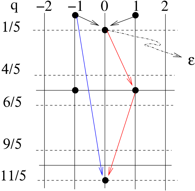
which associate at each field $\Phi^{q}$ , with conformal dimension $\Delta_{q}^{\Phi}$ , the field $\Phi^{-q}$ with opposite charge and with the same conformal dimension, $\Delta_{q}^{\Phi}=\Delta_{-q}^{\Phi}$ . The eigenvalues $h_{q}$ defined in (38) characterize the representations of the parafermionic algebra together with the conformal dimension the fields $\Phi^{q}$ . As usual, primary fields are defined by $A^{k}_{-\delta^{q}_{k+q}+n}\Phi^{q}=0$ for $n>0$ . Each representation module is then characterized by the two primary fields $\Phi^{\pm q}$ which can be obtained one from the other as in (38). An example of the module structure associated to the field $\Phi^{\pm 1}$ and of the action of the currents is given in Fig.5 for $N=5$ . Using the formula (37), we have $\delta^{\pm 1}_{0}=1/5$ and $\delta^{\pm 1}_{\pm 2}=4/5$ .

Using the expansion (36), the action of the modes in each sector can be given in terms of a contour integral:

A^{k}_{-\delta^{q}_{k+q}+n}\Phi^{q}(0)=\frac{1}{2\pi i}\oint_{C_{0}}{\rm d}z\,(z)^{\Delta_{k}^{\Psi}-\delta^{q}_{k+q}+n-1}\Psi^{k}(z)\Phi^{q}(0).

(39)

In the $Z_{N}$ sector, one can simply consider the action of the currents $\{\Psi^{\pm 1}\}$ because, via the Eq. (28), they completely determine the full algebra of the other currents $\{\Psi^{\pm k}\}$ , $k=2,\cdots,\lfloor N/2\rfloor$ .

The commutation relations of the mode operators can be deduced from Eq.(39) by using standard techniques in the complex plane. These relations are given in Appendix B.1.

As shown in the Appendix B.1, the representation space contains $\lfloor N/2\rfloor$ +1 primary operators $\Phi^{q}$ with $q=0,1,\cdots,\frac{N}{2}$ for $N$ odd and with $q=0,\pm\frac{1}{2},\pm 1,\cdots,\pm\lfloor N/4\rfloor$ for $N$ even. The conformal dimension of these operators turn out to be:

\Delta_{q}^{\Phi}=\frac{q(N-2q)}{N(N+2)}\quad\,q=0,1,\cdots,\frac{N-1}{2}(N\,\mbox{odd}),\quad q=0,\frac{1}{2},1,\cdots,\frac{N}{4}\quad(N\,\mbox{even}).

(40)

As said above, to each primary $\Phi^{q}$ corresponds another primary field $\Phi^{-q}$ of the same dimension.

In the case $N=2$ and $N=3$ (i.e. Ising and three state Potts model), one has only two primaries of the parafermionic algebra. For $N=2$ one finds the identity operator with $\Delta_{0}=0$ and the operator $\Phi^{\pm 1/2}$ , with dimension $\Delta_{\pm 1/2}=1/16$ , corresponding to the Ising model spin operator. Analogously, for $N=3$ one has, together with the identity operator, the operator $\Phi^{\pm 1}$ with $\Delta_{\pm 1}=1/15$ . As previously said, the case $N=2$ and $N=3$ are special because they can be identified with the minimal model $M_{3}$ and $M_{5}$ . The operators $\Phi^{\pm 1/2}$ and $\Phi^{\pm 1}$ are identified respectively to the operators $\phi_{1,2}$ and $\phi_{2,3}$ of the corresponding $M_{3}$ and $M_{5}$ Kac tables, see Eq.(13). As we will show more in detail below, the representation module corresponding to $\Phi^{\pm 1}$ contains one descendant state, $\varepsilon^{(N=3)}=A^{-1}_{-1/3}\Phi^{+1}=A^{1}_{-1/3}\Phi^{-1}$ singlet under $Z_{3}$ transformation (i.e. $q=0$ ). This singlet (energy) operator has dimension $\Delta_{\varepsilon}=1/15+1/3=2/5$ , it is a primary of the Virasoro algebra and can be identified with the operator $\varepsilon^{(N=3)}=\phi_{2,1}$ of the $M_{5}$ Kac table.

IV.3 Representation space: the disorder sector.

A key observation is that the theory we are considering is actually invariant under the dihedral group $D_{N}$ which includes $Z_{N}$ as a subgroup. This can directly be seen from the symmetry of Eq.(28)-(32) under the conjugation of the $Z_{N}$ charge, $q\to N-q$ . At the level of the lattice model (see V), this comes from the invariance of the Hamiltonian under the transformation $\sigma_{k}(x)\to\sigma_{k}^{+}(x)$ .

The space of representation thus includes the $N-$ plet of $Z_{2}$ operators which we denote as:

\displaystyle\{R_{a}(z,\bar{z}),\quad a=1,\ldots,N\}.

(41)

In the following, we refer to these operators as disorder operators.

The theory of disorder operators has been fully developed in Zamo2. A detailed discussion about the general properties (products, analytic continuations) of these operators is given in Raoul1.

The most important feature of the disorder operators is their non-abelian monodromy with respect to the chiral fields $\{\Psi^{\pm k}\}$ . This amounts to the decomposition of the local products $\Psi^{k}(z)R_{a}(0)$ into half-integer powers of $z$ :

\Psi^{k}(z)R_{a}(0)=\sum_{n}\frac{1}{(z)^{\Delta_{k}^{\Psi}+\frac{n}{2}}}\,A^{k}_{\frac{n}{2}}R_{a}(0),\qquad k=1,2,\ldots,\lfloor N/2\rfloor.

(42)

The expansion of the product $\Psi^{-k}(z)R_{a}(0)$ (with $k=1,2,\ldots,\lfloor N/2\rfloor$ ) can be obtained by an analytic continuation of $z$ around 0 on both sides of Eq. (42). The result is:

\Psi^{-k}(z)R_{a}(0)=\sum_{n}\frac{(-1)^{n}}{(z)^{\Delta_{k}^{\Psi}+\frac{n}{2}}}A^{k}_{\frac{n}{2}}\,R_{a-k}(0),\qquad k=1,2,\ldots,\lfloor N/2\rfloor.

(43)

In accordance with these expansions, the mode operators $A^{k}_{\frac{n}{2}}$ can be defined by the contour integrals

A^{k}_{\frac{n}{2}}R_{a}(0)=\frac{1}{4\pi i}\oint_{C_{0}}{\rm d}z\,(z)^{\Delta_{k}^{\Psi}+\frac{n}{2}-1}\Psi^{k}(z)R_{a}(0),

(44)

where the integrations are defined by letting $z$ turn twice around the operator $R_{a}(0)$ at the origin, exactly as described in Zamo2; Raoul1. The commutation relations between the current modes in this sector can be computed and the dimension of the primary disorder operators is (see Appendix B.4):

\Delta^{R}_{s}=\frac{N-2+(N-2s)^{2}}{16(N+2)}\quad s=0,1,\cdots,\lfloor N/2\rfloor.

(45)

Note that for $N=2$ one has the operators $R_{a}^{(0)}$ and $R_{a}^{(1)}$ with dimension $\Delta^{R}_{0}=1/16$ and $\Delta^{R}_{1}=0$ . This is of course expected as the dihedral group $D_{2}=Z_{2}$ , i.e. the cyclic $Z_{N}$ elements and the reflection $Z_{2}$ elements of the group $D_{N}$ coincide for $N=2$ . In particular one has $R_{a}^{0}=\Phi^{\pm 1/2}$ while $R_{a}^{1}$ coincides with the identity. For $N=3$ , the disorder sector contains the operator $R_{a}^{0}$ ( $\Delta^{R}_{0}=1/8$ ) and $R_{a}^{1}$ ( $\Delta^{R}_{1}=1/40$ ). In terms of primaries of the Virasoro algebra they coincide respectively with the $\phi_{1,2}$ and $\phi_{2,2}$ operators of the $M_{5}$ Kac table, see again Eq.(13).

IV.4 Stochastic motion in the internal space.

We discuss now a possible SLE approach to describe parafermionic theories. In the previous section we have seen that the action (39) and (44) of the chiral currents modes on the representation fields amounts to a twist either of the $Z_{N}$ charge $q$ for fields $\Phi^{q}(z)$ belonging to the $Z_{N}$ sector, or of the $Z_{2}$ index $a$ for fields $R_{a}(z)$ in the disorder sector. The b.c.c. operator is expected to transform as an operator in the $Z_{N}$ or in the $Z_{2}$ sector. By analogy to the case of the $SU(2)_{N}$ WZW Ludwig, we consider an independent stochastic motion in the additional degrees of freedom. We provide a parafermionic field the following evolution:

X(z)\to X(z)+\frac{1}{2\pi i}\oint_{\mathcal{C}_{z}}d\,g_{t}(w)T(w)X(z)+\frac{1}{2\pi i}\oint_{\mathcal{C}_{z}}d\,w(d\theta)^{k}(w)\Psi^{k}(w)X(z),

(46)

where $X(z)=\Phi^{q}$ or $X(z)=R_{a}(z)$ and the contour $\mathcal{C}_{z}$ is a general closed contour around $z$ (remember that in the $R$ sector the Riemann surface is two-fold). This evolution contains, in addition to the variation under an infinitesimal conformal transformation $dg_{t}(w)$ , a component with shifted $Z_{N}$ charge $q\to q+k$ or $Z_{2}$ charge, $a\to a+k$ . The (46) can be seen as a motion in the parafermionic representation module. In the sequel, we shall concentrate on considering only the action of the most fundamental $\Psi^{\pm 1}$ fields.

The definition of the internal stochastic motion is given in such a way that the corresponding Ito derivative of $\psi(z)$ takes the form (7) or (24). More precisely, we want to derive a martingale condition as a linear relation between descendants at the level two of some representation module. This allows for a direct comparison with the CFT results.

In the case the boundary operator $\psi(z)$ coincides with a primary $\Phi^{q}$ in the $Z_{N}$ sector, we define:

(d\theta)_{t}^{k}(z)=\frac{(d\theta)^{k}_{t}}{(g_{t}(z)-\xi_{t})^{-\Delta_{k}^{\Psi}+\delta^{q}_{k+q}+1}},\quad\mbox{{\bf E}}[\theta^{k}_{t}\theta^{k^{\prime}}_{s}]=\tau\,\delta^{k,-k^{\prime}}\,\mbox{min}(s,t).

(47)

The exponent in the denominator has been chosen according to Eq.(36) which encodes the OPE between the currents $\Psi^{k}$ and the fields $\Phi^{q}$ . Note that this evolution is very similar to (23) in the $su(2)$ Lie algebra. This is somehow expected since the $Z(N)$ parafermionic theory corresponds to the coset $SU(2)_{N}/U(1)$ (see appendix A).

In the case when $\psi(z)$ transforms as a disorder $R_{a}$ field, we define, according to Eq.(42):

(d\theta)_{t}^{k}(z)=\frac{(d\theta)^{k}_{t}}{(g_{t}(z)-\xi_{t})^{-\Delta_{k}^{\Psi}+2}},\quad\mbox{{\bf E}}[\theta^{k}_{t}\theta^{k^{\prime}}_{s}]=\tau\,\delta^{k,-k^{\prime}}\,\mbox{min}(s,t).

(48)

We point out that the definition of the stochastic motion given above is by now purely algebraic and based on a formal analogy with the case $SU(2)$ . However, the CFT predictions and the identification of the possible interface on the lattice model motivate the interest of such construction.

IV.5 Martingale conditions and parafermionic results.

As we will discuss in some detail later, the Ising model ( $N=2$ and $c=1/2$ ) shows in its FK representation (see V) a domain wall described by the SLE_16/3. The b.c.c operator creating such interface is identified with the operator $\phi_{1,2}$ of the $M_{3}$ Kac table, what is consistent with the Eq.(17) and Eq.(18). In the parafermionic representations, we have seen that this operator corresponds to the disorder $R_{a}^{(0)}$ operator or, equivantely, to the $\Phi^{\pm 1/2}$ operator (remember that $N=2$ is special as $D_{2}$ = $Z_{2}$ ). In the three state Potts model ( $N=3$ ), the operator $\phi_{1,2}$ of the $M_{5}$ Kac table is again identified again with the disorder $R_{a}^{(0)}$ and it is expected to create an SLE_24/5, in agreement again with Eq.(17) and Eq.(18). The operator $\phi_{2,1}$ , on the other hand, can be associated to an interface described by the SLE_10/3 and it corresponds to the $\varepsilon^{(N=3)}=A^{1}_{-1/3}\Phi^{-1}=A^{-1}_{-1/3}\Phi^{1}$ operator mentioned before.

On the basis of these correspondences, it is then natural to identify for general $N$ the b.c.c. operator $\psi(z)$ with the disorder primary operator $R_{a}^{(0)}$ with dimension $\Delta_{0}=(N^{2}+N-2)/(16(N+2))$ and with the $Z_{N}$ singlet (i.e. charge $q=0$ ) operator $\varepsilon^{(N)}=A^{-1}_{-1/N}\Phi^{1}=A^{1}_{-1/N}\Phi^{-1}$ with dimension $\Delta_{\varepsilon}=2/(N+2)$ . Note that this singlet operator is not a primary of the parafermionic algebra but it appears as descendant in the module of $\Phi^{\pm 1}$ (see appendix B).

Using Eq.(30), Eq.(37) and Eq.(46), the stochastic motions (47) and (48) amounts respectively to the following dynamics for $\psi(z)$ in the two cases when $\psi(z)\equiv\psi_{\varepsilon}=\varepsilon(z)$ and $\psi(z)\equiv\psi_{R}=R_{a}^{(0)}$ :

	$\displaystyle d(\psi_{\varepsilon}(\xi_{t}))=d\xi_{t}L_{-1}\psi_{\varepsilon}(\xi_{t})+(d\theta)^{1}A^{1}_{1/N-1}\psi_{\varepsilon}(\xi_{t})+(d\theta)^{-1}A^{-1}_{1/N-1}\psi(\xi_{t})_{\varepsilon}$
	$\displaystyle+dt\left(\frac{\kappa}{2}L_{-1}^{2}+\frac{\tau}{2}\left[A^{1}_{-1/N-1}A^{-1}_{1/N-1}+A^{-1}_{-1/N-1}A^{1}_{1/N-1}\right]\right)\psi_{\varepsilon}(\xi_{t}).$		(49)

and $\psi(z)\equiv\psi_{R}=R_{a}^{(0)}$ :

	$\displaystyle d(\psi_{R}(\xi_{t}))=d\xi_{t}L_{-1}\psi_{R}(\xi_{t})+(d\theta)^{1}A^{1}_{-1}\psi_{R}(\xi_{t})+(d\theta)^{-1}A^{-1}_{-1}\psi_{R}(\xi_{t})$
	$\displaystyle+dt\left(\frac{\kappa}{2}L_{-1}^{2}+\frac{\tau}{2}\left[A^{1}_{-1}A^{-1}_{-1}+A^{-1}_{-1}A^{1}_{-1}\right]\right)\psi_{R}(\xi_{t}).$		(50)

The martingale condition, to be compared with Eq.(14) and Eq.(25), now reads:

	$\displaystyle\left(L_{-2}-\frac{\kappa}{4}L_{-1}^{2}-\frac{\tau}{4}\left[A^{1}_{-1/N-1}A^{-1}_{1/N-1}+A^{-1}_{-1/N-1}A^{1}_{1/N-1}\right]\right)\psi_{\varepsilon}(\xi_{t})$	$\displaystyle=$	$\displaystyle 0$		(51)
	$\displaystyle\left(L_{-2}-\frac{\kappa}{4}L_{-1}^{2}-\frac{\tau}{4}\left[A^{1}_{-1}A^{-1}_{-1}+A^{-1}_{-1}A^{1}_{-1}\right]\right)\psi_{R}(\xi_{t})$	$\displaystyle=$	$\displaystyle 0.$		(52)

We can now enounce the main results of this paper. We have studied the representation modules of the $\varepsilon$ and $R_{a}^{(0)}$ operator. For $N\geq 4$ one finds that there are at least two independent states at the second level of these operators. We have found the following relations at the second level of these modules:

	$\displaystyle\left(L_{-2}-\frac{N+1}{N+2}L_{-1}^{2}-\frac{N^{3}}{(N+2)^{3}}\left[A^{1}_{-1/N-1}A^{-1}_{1/N-1}+A^{-1}_{-1/N-1}A^{1}_{1/N-1}\right]\right)\psi_{\varepsilon}(\xi_{t})$	$\displaystyle=$	$\displaystyle 0$		(53)
	$\displaystyle\left(L_{-2}-\frac{N+2}{N+1}L_{-1}^{2}-\frac{2^{-4/N}N^{3}}{4(N+2)(N+1)}\left[A^{1}_{-1}A^{-1}_{-1}+A^{-1}_{-1}A^{1}_{-1}\right]\right)\psi_{R}(\xi_{t})$	$\displaystyle=$	$\displaystyle 0,$		(54)

The derivation of these relations is shown in appendix B. We have verified that, for $N=2$ , the relation (54) reduces to (15) and for $N=3$ , the Eq.(53) and Eq.(54) are respectively equivalent to Eq.(16) and Eq.(15). In these cases, which as already said coincide with minimal models $M_{3}$ and $M_{5}$ , all the descendants of the theory can be obtained by applying negative Virasoro modes. In our case, this amounts to the fact that the states at the second level constructed from the application of parafermionic modes can be written as a linear combination of $L_{-1}^{2}$ and $L_{-2}$ .

Comparing Eq.(51) and Eq.(52) to Eq.(53) and Eq.(53), we obtain, for $N\geq 4$ and for the two SLEs evolutions:

	$\displaystyle\kappa_{1}$	$\displaystyle=$	$\displaystyle 4\frac{N+1}{N+2}\quad\tau_{1}=4\frac{N^{3}}{(N+2)^{3}}$		(55)
	$\displaystyle\kappa_{2}$	$\displaystyle=$	$\displaystyle 4\frac{N+2}{N+1}\quad\tau_{2}=2^{-4/N}\frac{N^{3}}{(N+2)(N+1)}$		(56)

V $Z(N)$ self-dual critical spin models.

Consider a square lattice with the spin variables $\sigma_{j}$ at each sites $j$ taking $N$ possible values:

\sigma_{j}=\exp\left[\frac{i2\pi}{N}n(j)\right]\quad n(j)=0,1,\cdots,N-1.

(57)

The most general $Z_{N}$ -invariant spin model with nearest-neighbor interactions is defined by the reduced Hamiltonian Zama_lat; Dotsi_lat; Fradkin_lat:

H[n]=-\sum_{m=1}^{\lfloor N/2\rfloor}J_{m}\left[\cos\left(\frac{2\pi mn}{N}\right)-1\right].

(58)

and the associated partition function reads:

Z=\sum_{\{\sigma\}}\exp\left[-\beta\sum_{<ij>}H[n(i)-n(j)]\right]

(59)

In fact, the Potts model is recovered in the case $J_{m}=J$ for all $m$ . The model presents, in this case, a permutational $S_{N}$ symmetry. Another meaningful model is the clock model which is defined by the partition function (59) with $J_{m}=J\delta_{m,1}$ . Defining the Boltzmann weights:

x_{n}=\exp\left[-\beta H(n)\right],\quad n=0,1,\cdots,N-1,

(60)

the general $Z(N)$ spin system is described by $\lfloor N/2\rfloor$ independent parameters $x$ . The Kramers and Wannier (order-disorder) duality has proven to be a powerful tool for examining the behavior of these models. The phase diagram of the model (59) for $N=5$ states of spin is shown in Fig.(2). It has been show that the $Z(5)$ model is self-dual on the line $x_{1}+x_{2}=1/2(\sqrt{5}-1)$ . Here we are interested in the existence of two critical points $(x_{1}^{*},x_{2}^{*})$ and $(x_{2}^{*},x_{1}^{*})$ , where $x_{1}^{*}=\sin(\pi/20)/\sin(3\pi/20)\approx 0.34$ and $x_{2}^{*}=\sin(\pi/4)/\sin(7\pi/20)x_{1}^{*}\approx 0.27$ , where the model is completely integrable. The $Z(5)$ parafermionic theory defined in the previous sections describes the continuum limit of the lattice model at these points. In general, in the self-dual subspace of (58)-(59), which contains also the Potts model the clock model, the $Z(N)$ spin model is completely integrable at the points Zama_lat2 :

	$\displaystyle x^{*}_{0}$	$\displaystyle=$	$\displaystyle 1$
	$\displaystyle x^{*}_{n}$	$\displaystyle=$	$\displaystyle\prod_{k=0}^{n-1}\sin\left(\frac{\pi k}{N}+\frac{\pi}{4N}\right)\left[\sin\left(\frac{\pi(k+1)}{N}-\frac{\pi}{4N}\right)\right]^{-1}.$		(61)

These critical points are described by the $Z(N)$ parafermionic field theories.

V.1 Boundary conditions and SLE interfaces.

Consider the three-states Potts model. From the Eq.(17) and the Eq.(18), as previously mentioned, the b.c.c. operator $\psi_{\varepsilon}^{(N=3)}$ is expected to create an SLE_10/3 trace. In this paragraph we suggest a definition of the interfaces within the lattice models whose scaling limit is described in these SLE processes. In the following we indicate the possible values of the spins with the letters $A,B\cdots$ . The b.c.c. operator $\psi_{\varepsilon}^{(N=3)}$ has been shown to generate the boundary condition where the spins are fixed to (say) the value $A$ on the left side of the origin while can take the value $B$ or $C$ with equal probability on the right side Cardy_bcft2. With this boundary condition, to which we refer with the short-hand notation $A|B+C$ , there exists a single domain wall between the spin $A$ and the spins $B$ and $C$ , as shown in Fig.1. The statistical properties of this interface has recently been analyzed by numerical means in Cardy_potts and are shown to be well described in the continuum limit by an SLE_10/3.

Refer to caption — Figure 1: a)Three state Potts model: interface (green curve) between the $A$ spins (black circles) and the $B$ (full blue circles) and $C$ (empty blue circles). The boundary conditions $A|B+C$ as in the text. b) The interface defined in the $Z(5)$ spin model with boundary conditions $A|B+C+D+E$ .

The generalization to the $N$ -states spin model is straightforward. Indeed, one can show (see appendix C) that the b.c.c. operator $\psi_{\varepsilon}^{(N)}$ produces the boundary conditions $A|B+C+D+\cdots$ , where the spins on the left of the origin take the value $A$ while the ones on the right take with equal probability the $N-1$ values of spin different from $A$ . As in the case of $N=3$ , there exists a single boundary domain between the $A$ spin and the $B,C,\cdots..$ . Note that the boundary conditions do not satisfy the reflection symmetry and the measure on the curve should reflect this asymmetry. However, in the continuum limit the reflection symmetry is expected to be restored as explicitely shown in Cardy_potts. This can be argued from the fact that, in this limit, the statistical expectation values can be expressed in terms of CFT correlation functions which contain the b.c.c. operators, see Eq.(4). These correlation functions satisfy indeed the reflection symmetry.

It is interesting to note that one can assign a “color” to the interface depending on the values of the spins ( $B,C,\cdots$ ) at the right of the domain wall. The point is that, for $N<4$ , the Boltzmann weights $x_{n}^{*}$ , $n=1,2,\cdots,N-1$ , are equal: the energy of one bond does not depend on the difference between the values of the nearest-neighbor spins. In this sense, the $Z_{N}$ symmetry is trivially realized and this is essentially the reason why, for $N=2,3$ , the correspondent CFT can be constructed from the conformal invariance alone. However this is not true for $N\geq 4$ where the Boltzmann weights $x_{n}^{*}$ , $n=1,2,\cdots\lfloor N/2\rfloor$ are different. In the continuum limit, this amounts to a more structured chiral algebra with a central charge $c\geq 1$ . From the point of view of the lattice model, one can observe that for $N=2,3$ the energy cost to have a spin $B$ or $C$ at one side of the interface is the same. Thus, as $N\geq 4$ , one expects the internal spin degree of freedom to play an important role in the spatial evolution of the interface. This is somehow in agreement with the need to introduce an additional stochastic motion in the $Z_{N}$ group. However a clear the geometrical interpretation of the stochastic evolution in the representation modules (see section IV.4) is missing.

From the results (53) and (55), we hypothesize that the geometric properties of this interface for $N\geq 4$ are described by a $SLE$ with $\kappa=4(N+1)/(N+2)$ . In particular, since $\kappa\leq 4$ , we expect the domain under consideration to be a simple curve for each $N$ .

We discuss now the identification of the interface on the lattice associated to the b.c.c operator $\psi_{R}$ , see Eq.(54). In the Ising and three states Potts model, this operator is associated to an SLE_16/3 and SLE_24/5 respectively. The correspondent interfaces on the lattice can be identified with the help of the Fortuin-Kasteleyn (FK) representations.

The partition function (59) for the $N=2$ and $N=3$ critical models take the form:

Z=\sum_{\{\sigma\}}\exp\left[-\beta\sum_{<ij>}H(n(i)-n(j))\right]=\sum_{\{\sigma\}}\prod_{<ij>}\left[x_{1}^{*}+(1-x_{1}^{*})\delta_{n(i),n(j)}\right],

(62)

where $x_{1}^{*}=\sqrt{2}-1$ or $x_{1}^{*}=x_{-1}^{*}=(\sqrt{3}-1)/2$ is the critical point of the Ising and of the three states Potts model respectively. By expanding the product (62) and summing over all the spin configurations, one obtains the FK random cluster representation:

Z=\sum_{\mathcal{C}}(x_{1}^{*})^{M-b}(1-x_{1}^{*})^{b}N^{c}

(63)

where the sum is over the subgraphs $\mathcal{C}$ of $\mathcal{G}$ , $\mathcal{C}\subseteq\mathcal{G}$ , the graph $\mathcal{G}=(V,E)$ being composed by the $V$ sites and the $E$ edges of the square lattice. Each graph $\mathcal{C}$ is specified by the $b$ bonds on the edges and the $c$ clusters (=connected component which include the single sites) in a given bond configuration.

Consider the following boundary conditions: all the edges on the negative axis carry bonds while all the edges on the positive axis carry no bonds. For the spin variables this means that all the spins located at the left of the origin take the same value while the spins on right side are unconstrained, i.e. they are free (F) to take all the $N$ possible values.

In such an arrangement, each graph $\mathcal{C}$ presents a cluster growing from the negative axis into the upper half-plane. The boundary of this cluster, starting from the origin, is conjectured (see for istance Walter, chapter 5) to be statistically equivalent in the continuum limit to the SLE_16/3 for $N=2$ (Ising model) and to the SLE_24/5 for $N=3$ (the three states Potts model). This is in agreement with the properties of the b.c.c. $\psi_{R}^{(N)}$ operators, $N=2,3,4$ , which have been shown Bauer_R to be associated to the $A|F$ boundary conditions.

The generalization to the case $N\geq 4$ is more cumbersome. To our knowledge, the modular properties of the $R-$ sector characters, and thus the boundary conditions associated to these operators, have not been yet studied for these cases. This motivates a more detailed analysis of the boundary conformal properties of this sector. However, we point out that at the level of the parafermionic algebra representations the main features of the $\psi_{R}$ fields, such as the structure and the degeneracies of the representation module or the current zero modes eigenvalues (see Appendix B.4), directly generalize to each $N\geq 2$ . The formula (45) is an example. It is thus quite natural to suppose that the operators $\psi_{R}^{(N)}$ produce the $A|F$ boundary conditions for each $N$ . Another observation is that it is quite direct to find an alternative formulation of (59) in terms of colored clusters on a graph. For sake of clarity, we focus our attention on the case $N=5$ .

The partition function (59) for $N=5$ at the critical point $x_{n}^{*}$ , see Eq.(61), can be rewritten as:

Z^{(N=5)}=\sum_{\{\sigma\}}\prod_{<ij>}\left[x_{1}^{*}+(1-x_{1}^{*})\delta_{n(i),n(j)}+(x_{2}^{*}-x_{1}^{*})\delta_{n(i),n(j)\pm 2}\right].

(64)

If $x_{1}^{*}=x_{2}^{*}$ one recovers the five states Potts model in the usual FK representation.

Expanding the factors in (64), one has to take into account two type of bonds: the bonds (type 1) connecting spins which take equal values and the bonds (type 2) connecting spins which differ by an angle $4\pi/5$ . Then, summing over the spin configurations, the partition function can be cast in terms of a sum over “colored” graphs $\mathcal{C^{\prime}}$ :

Z^{(N=5)}=\sum_{\mathcal{G^{\prime}}}(x_{1}^{*})^{E-b_{1}-b_{2}}(1-x_{1}^{*})^{b_{1}}(x_{2}^{*}-x_{1}^{*})^{b_{2}}5^{c}.

(65)

Each graph $\mathcal{C^{\prime}}$ is specified by the number $c$ of connected component and by the numbers $b_{1}$ and $b_{2}$ of the bonds of type 1 and type 2. Naturally, the sum over the differences of the spins along a loop must be zero (modulo $2\pi$ ). For instance, a loop formed by three bonds of type 2 and one bond of type 1 is not permitted. The prime in $\mathcal{C^{\prime}}$ indicates that the sum in (65) is taken over the allowed graphs. A typical configuration is shown in Fig.(3).

By analogy to the Ising and three states Potts model, we consider the boundary conditions in which the spins have a fixed value on the negative axis while they are free on the positive axis. With such boundary conditions, there is a cluster of bonds of type $1$ growing from the negative axis, see Fig.(4) .

From (56), we conjecture the geometric properties of the boundary of this cluster are described in the continuum limit by the SLE_14/3.

The above discussion can be directly generalized to each value of $N$ . In particular, the $Z(N)$ spin model admits a random cluster representations with $\lfloor(N-1)/2\rfloor$ types of bonds. Imposing the conditions on the real axis discussed above, we conjecture that the measure of the boundary of the cluster growing from the negative real axis is described by an SLE with $\kappa=4(N+2)/(N+1)$ .

Finally we remark that, during its evolution, the interface crosses edges without bonds or with bonds of the type $2,3,\cdots\lfloor(N-1)/2\rfloor$ which have different energetic costs. Analogously to the case of the interface generated by the $A|B+C+\cdots$ boundary conditions, one can color the interface depending on the type of bond it crosses. Again, the interface is naturally provided of an $Z_{N}$ additional internal degree of freedom, in agreement with the approach proposed in Section (IV.4).

VI Conclusions.

In this paper we have considered the possibility to extend an SLE approach to CFTs with additional $Z_{N}$ discrete symmetries. These theories describe the continuum limit of the self-dual critical $Z(N)$ spin models. The case $N=2$ and $N=3$ correspond to the Ising and three states Potts model where the identification of the interface on the lattice and of the correspondent b.c.c. operators are known. Using these results, we have identified the possible b.c.c. operators for general $N$ . We show that these operators satisfy a two level null vector condition. For $N\geq 4$ , an additional term enter these relations. This term is obtained from the action of the parafermionic currents and, for $N\geq 4$ ( $c\geq 1$ ), it cannot be derived by the Virasoro modes action. These results led us to propose an additional stochastic motion in the different $Z_{N}$ charge sectors and in the $Z_{2}$ sectors which describe the representation modules of the parafermionic algebra. We have finally discussed the possible interfaces in the lattice to which the CFT/SLE results should apply. The fact that SLE candidates have been identified in lattice spin models described by non-conformal minimal theories opens the possibility to study the SLE/non-minimal CFT connection by a numerical approach.

It will be interesting to verify our predictions by numerical studies. Further we believe these studies can also better clarify the geometrical interpretation of the additional stochastic motion in the internal space.

Acknowledgments: We would like to thank M. Bauer, J. Cardy, I. Gruzberg, C. Hagendorf, A. Ludwig, V. Riva for very helpful discussions. We are particularly grateful to D. Bernard and P. Le Doussal for very useful advises and support all along this work.

Appendix A Relation between the $SU(2)_{N}$ WZW model and the $Z(N)$ parafermionic theory.

In this appendix we briefly show how the stochastic motion (23) for the $SU(2)_{N}$ WZW theories can be somehow compared to the one (47) by taking into account that the $Z(N)$ parafermionic theory corresponds to the coset $SU(2)_{N}/U(1)$ . The $SU(2)_{N}$ WZW theory can then be seen as a combined system of the $Z_{N}$ parafermionic theory and one free massless boson field $\phi(z)$ . The chiral currents generating the Kac-Moody algebra (19) can be written in terms of the parafermionic currents and the free field as:

	$\displaystyle J^{\pm}$	$\displaystyle=$	$\displaystyle\sqrt{N}\Psi^{\pm 1}(z)\exp\left[\pm i\frac{1}{\sqrt{N}}\phi(z)\right]$
	$\displaystyle J^{0}$	$\displaystyle=$	$\displaystyle i\frac{\sqrt{N}}{2}\partial\phi(z).$		(66)

The stress-energy tensor $T^{SU(2)_{N}}$ and $T^{Z(N)}$ of the two theories are symply related by $T^{SU(2)_{N}}=T^{Z(N)}+T^{U(1)}$ , where $T^{U(1)}=-1/4(\partial\phi)^{2}$ is the stress-energy tensor of the free bosonic theory.

All the primary fields $\phi_{j}$ of the $WZW$ theory can be obtained by a product of parafermionic fields in the $Z_{N}$ sector and of vertex operators of the bosonic theory:

\phi_{j}(z)=\Phi^{j}\exp\left[i\frac{j}{\sqrt{N}}\phi(z)\right].

(67)

Using the fact that the conformal dimension $\Delta^{vert.}_{\alpha}$ of the vertex operator $\exp[\pm i\alpha\phi(z)/\sqrt{N}]$ is $\Delta^{vert.}_{\alpha}=\alpha^{2}/N$ , one can easily verify that $\Delta_{j}=\Delta^{\Phi}_{j}+\Delta^{vert.}_{j}$ , see Eq. (21) and Eq (40). Note that the field $\phi_{j}(z)$ in Eq.(67) satisfies $J^{0}_{0}\phi_{j}=j\phi^{m}_{j}$ . In the following we denote $\phi^{m}_{j}(z)$ , with $m=-j,-j+1,\cdots,j$ , the field in the $SU(2)$ representation of spin $j$ such that $J^{0}_{0}\phi^{m}_{j}=m\phi^{m}_{j}$ . The field $\phi^{j-k}_{j}$ can be expressed in terms of the parafermionic primaries $\Phi^{q}$ and of vertex operators as:

\phi^{j-k}_{j}(z)=(A^{-k}_{-\delta^{j}_{j-k}}\Phi^{j})\exp\left[i\frac{j-k}{\sqrt{N}}\phi(z)\right].

(68)

where $\delta^{q}_{k}$ has been defined in Eq.(37). For instance, the $SU(2)$ operator $\phi_{1}^{0}$ corresponds to $\varepsilon^{(N)}$ , see section IV.5, while the operator $\phi_{\pm 1}^{1}$ to $\Phi^{\pm 1}\exp[\pm i\phi(z)]$

Using the above relations, one can compare the definitions (23) and (47), and in particular the exponent in the denominator of the two formulas. This exponent actually determines the current mode acting on the b.c.c. field under his evolution. In the $SU(2)_{N}$ theory this is the $J^{a}_{-1}$ mode, as it can be seen in Eq.(24). Let us consider for istance the state $J^{-}_{-1}\phi^{1}_{1}$ :

$\displaystyle J^{-}_{-1}\phi^{1}_{1}$	$\displaystyle=$	$\displaystyle 1/(2\pi i)\oint_{w}dz\,(z-w)^{-1}\,J^{-}(z)\phi^{1}_{1}(w)$	(69)
		$\displaystyle\propto 1/(2\pi i)\oint_{w}dz(z-w)^{-1}\left(\Psi^{-1}(z)\Phi^{1}(w)\right)\left(\exp\left[\frac{-i}{\sqrt{N}}\phi(z)\right]\exp\left[\frac{i}{\sqrt{N}}\phi(w)\right]\right)$
	$\displaystyle\propto$	$\displaystyle 1/(2\pi i)\oint_{w}dz(z-w)^{-1-2/N}\left(\Psi^{-1}(z)\Phi^{1}(w)\right)\left(1+\frac{i}{\sqrt{N}}(z-w)\partial\phi(w)+\cdots\right),$

where we have used the relations (67) and the divergences coming from the OPE in the bosonic sector:

\exp\left[i\frac{q}{\sqrt{N}}\phi(z)\right]\exp\left[i\frac{q^{\prime}}{\sqrt{N}}\phi(z^{\prime})\right]=(z-z^{\prime})^{2\frac{q\,q^{\prime}}{N}}\exp\left[i\frac{q+q^{\prime}}{\sqrt{N}}\phi(z^{\prime})\right]+\cdots

(70)

The above expression gives precisely the state $A^{-1}_{-1/N-1}\Phi^{1}$ multiplied by a bosonic piece. In the same way one can show that the term $J^{-}_{-1}\phi^{0}_{1}$ and the term $(J^{+}_{-1}J^{-}_{-1}+J^{-}_{-1}J^{+}_{-1})\phi^{0}_{1}$ correspond respectively to $A^{-1}_{1/N-1}\varepsilon^{(N)}$ and to $(A^{1}_{-1/N-1}A^{-1}_{1/N-1}+A^{-1}_{-1/N-1}A^{1}_{1/N-1})\varepsilon^{(N)}$ which also appear in the Ito derivative of the $Z(N)$ b.c.c. parafermionic operator, see Eq.(49).

Appendix B Null vectors in the parafermionic modules.

B.1 Commutation relations of parafermionic current modes: $Z_{N}$ sector

The commutation relations of the mode operators can be deduced from Eq.(39) by using standard techniques in the complex plane. Consider for instance the commutation relation of the modes of $\Psi^{1}(z)$ in the $Z_{N}$ singlet sector $\Phi^{0}$ . We use the short-hand notation $\{\Psi^{1},\Psi^{1}\}\Phi^{0}$ to indicate such relations. One consider the double integral:

\frac{1}{2\pi i}\oint_{C_{0}}{\rm d}z_{1}\oint_{C_{0}}{\rm d}\,z_{2}\,z_{1}^{n}z_{2}^{m}(z_{1}-z_{2})^{2/N-1}\Psi^{1}(z_{1})\Psi^{1}(z_{2})\Phi^{0}(0),

(71)

where one adds the term $(z_{1}-z_{2})^{2/N-1}$ to make the integrand single-valued. By using the Eqs.(28)-(36) and expanding in series the term $(z_{1}-z_{2})^{2/N-1}$ , the Cauchy theorem gives the following relations for $\{\Psi^{1},\Psi^{1}\}\Phi^{0}$ :

\sum_{l}D^{l}_{(2-N)/N}\left[A^{1}_{(3-N)/N+n}A^{1}_{1/N+m}+A^{1}_{(3-N)/N+m}A^{1}_{1/N+n}\right]\Phi^{0}=\lambda^{1,1}_{2}A^{2}_{(4-N)/N+n+m}\Phi^{0}.

(72)

The coefficients $D^{l}_{\alpha}$ are defined from the development

(1-x)^{\alpha}=\sum^{\infty}_{l=0}D^{l}_{\alpha}x^{l}.

(73)

The relations $\{\Psi^{1}\Psi^{-1}\}\Phi^{1}$ , for instance, are derived from the double integral:

\frac{1}{2\pi i}\oint_{C_{0}}{\rm d}z_{1}\oint_{C_{0}}{\rm d}\,z_{2}\,z_{1}^{2/N+n}z_{2}^{(N-2)/N+m}(z_{1}-z_{2})^{-(N+2)/N}\Psi^{1}(z_{1})\Psi^{-1}(z_{2})\Phi^{1}(0).

(74)

The exponent of the $(z_{1}-z_{2})$ term has been chosen on the basis of the OPE (29). In particular it allows the modes of the stress energy, appearing at the second order in (29), to enter in the relation $\{\Psi^{1}\Psi^{-1}\}\Phi^{\pm 1}$ . One obtains:

\sum_{l}D^{l}_{-(N-2)/N}\left[A^{1}_{1/N+n-1}A^{-1}_{-1/N+m+1}+A^{-1}_{-3/N+m}A^{1}_{3/N+n}\right]\Phi^{\pm 1}=\left[\frac{1}{2}\left(\frac{2}{N}+n\right)\left(\frac{2}{N}+n-1\right)\delta_{n+m,0}+\frac{N+2}{N}L_{n+m}\right]\Phi^{\pm 1}.

(75)

From the above relations, and using the primary condition (36), one can readily obtain the conformal dimension $\Delta_{1}$ of a primary field $\Phi^{\pm 1}$ . Setting $n=m=0$ in Eq.(75), one obtains $\Delta^{\Phi}_{1}=(N-2)/(N(N+2))$ .

For completeness, we give below in a compact form the the commutation relations $\{\Psi^{1},\Psi^{1}\}\Phi^{q}$ and $\{\Psi^{1},\Psi^{-1}\}\Phi^{q}$ which determine the space of the representations :

	$\displaystyle\sum^{\infty}_{l=0}D^{l}_{(2-N)/N}\left(A^{1}_{-\delta^{q+1}_{q+2}+s(q)+n-l}A^{1}_{-\delta^{q}_{q+1}+m+l}+A^{1}_{-\delta^{q+1}_{q+1}+s(q)+m-l}A^{1}_{-\delta^{q}_{q+1}+n+l}\right)\Phi^{q}=\lambda^{1,1}_{2}A^{2}_{-\delta^{q}_{q+2}+t(q)+n+m}\Phi^{q}$		(76)
	$\displaystyle\sum^{\infty}_{l=0}D^{l}_{-(2+N)/N}\left(A^{1}_{-\delta^{q-1}_{q}+u(1,q)+n-l}A^{-1}_{-\delta^{q}_{q-1}+m+l}+A^{-1}_{-\delta^{q+1}_{q}+u(-1,q)+m-l}A^{1}_{-\delta^{q}_{q+1}+n+l}\right)\Phi^{q}=$
	$\displaystyle=\left[\frac{1}{2}(\frac{2\|q\|}{N}+n)(\frac{2\|q\|}{N}+n-1)+\frac{N+2}{N}L_{n+m-1+u(1,q)}\right]\Phi^{q}.$		(77)

The integers $s(q)$ , $t(q)$ and $u(\pm 1,q)$ shift the indeces of the parafermionic modes:

$\displaystyle s(q)$	$\displaystyle=$	$\displaystyle\delta^{q+1}_{q+2}-\delta^{q}_{q+1}+\frac{2}{N}-1$
$\displaystyle t(q)$	$\displaystyle=$	$\displaystyle\delta^{q}_{q+2}-2\delta^{q}_{q+1}+\frac{2}{N}-1$
$\displaystyle u(k,q)$	$\displaystyle=$	$\displaystyle\delta^{q-k}_{q}-\delta^{q}_{q-k}-\frac{N+2}{N},$	(78)

where $\delta^{q}_{q+2}$ is defined in Eq.(37). Finally the algebra is then completed by the commutators between the parafermions modes $A^{\pm 1}$ and $L_{n}$ :

\left(A^{\pm 1}_{-\delta^{q}_{q\pm 1}+m}L_{n}-L_{n}A^{\pm 1}_{-\delta^{q}_{q\pm 1}+m}\right)\Phi^{q}=\left[(1-\Delta^{\Psi}_{1})n+m-\delta^{q}_{q\pm 1}\right]A^{\pm 1}_{-\delta^{q}_{q\pm 1}+m+n}\Phi^{q}..

(79)

Analogously to what we have seen above for the special case of the $\Phi^{\pm 1}$ field, the formula (40) giving the dimension of the primary fields is obtained by taking $n=m=0$ ( $n=1,m=0$ ) in the Eq.(77) for $q\neq 0$ ( $q=0$ ).

B.2 $\Phi^{\pm 1}$ module.

In the following we consider in more detail the module of the representation $\Phi^{\pm 1}$ . The structure of the corresponding module is shown in Fig.(5) for the case $N=5$ .

We have seen above that the dimension of the operator are given by the commutation relations Eq.(77) without imposing any degeneracy in the module. This in general is not the case, as it can be seen in the study of the representation of the minimal models or of other parafermionic algebras. However, in order to characterize completely the representation one needs to fix the eigenvalue $h_{\pm 1}$ of the zero mode defined in Eq.(38). We show this is easily obtained by imposing a degeneracy at level $1/N$ where the first descendent states in this doublet are the two singlet states $A^{-1}_{-1/N}\Phi^{+1}$ and $A^{1}_{-1/N}\Phi^{-1}$ . Forming the linear combination

\chi^{0}_{-\frac{1}{N}}=aA^{1}_{-\frac{1}{N}}\Phi^{-1}+bA^{-1}_{-\frac{1}{N}}\Phi^{1},

(80)

we wish to make it into a primary operator, i.e., to ensure that it is annihilated upon action by positive index mode operators. In this case it will be sufficient to verify that

A^{1}_{+\frac{1}{N}}\chi^{0}_{-\frac{1}{N}}=0\quad\mbox{and}\quad A^{-1}_{+\frac{1}{N}}\chi^{0}_{-\frac{1}{N}}=0.

(81)

The degeneracy conditions $A^{\pm 1}_{1/N}\chi^{0}_{-1/N}=0$ are satisfied if

\left(\mu_{1,1}\right)^{2}=\left(\mu_{1,-1}\right)^{2},

(82)

where the matrix element $\mu_{k,k^{\prime}}$ is defined by

\mu_{k,k^{\prime}}\Phi^{1}\equiv A^{k}_{1/N}A^{k^{\prime}}_{-1/N}\Phi^{-1}.

(83)

Using Eq.(28)-Eq.(29), one finds:

\mu_{1,1}=\lambda^{1,1}_{2}h_{1},\quad\mu_{1,-1}=\frac{2}{N},

(84)

where the structure constant $\lambda^{1,1}_{2}$ is given by Eq. (32), and the zero mode eigenvalue $h_{1}$ , defined in Eq. (38), is fixed to:

h_{1}^{2}=\frac{2}{N(N-1)}.

(85)

Once the conformal dimension and the zero eigenvalue Eq.(85) have been determined, the operator $\chi^{0}_{-\frac{1}{N}}=A^{1}_{-\frac{1}{N}}\Phi^{-1}-A^{-1}_{-\frac{1}{N}}\Phi^{1}$ is a primary operator and it is put to zero, $\chi^{0}_{-\frac{1}{N}}=0$ , to make the representation irreducible. After imposing the degeneracy at level $1/N$ , only one singlet state remains:

\varepsilon^{(N)}=A^{1}_{-\frac{1}{N}}\Phi^{-1}=A^{1}_{-\frac{1}{N}}\Phi^{-1},

(86)

with dimension

\Delta_{\varepsilon^{(N)}}=\frac{2}{N+2}.

(87)

B.3 Independent states at the second level of the $\varepsilon^{(N)}$ operator.

Using systematically the commutation relations Eq.(76)-Eq.(77), one can show that at the second level of the $\varepsilon^{(N)}$ operator there are only two independent states. All the operators at the second level can indeed be obtained by a linear combination of the following two states:

\left(A^{1}_{-\frac{1}{N}-1}A^{-1}_{\frac{1}{N}-1}+A^{-1}_{-\frac{1}{N}-1}A^{1}_{\frac{1}{N}-1}\right)\varepsilon^{(N)};\quad\mbox{and}\quad\left(A^{1}_{-\frac{1}{N}-2}A^{-1}_{\frac{1}{N}}+A^{-1}_{-\frac{1}{N}-2}A^{1}_{\frac{1}{N}}\right)\varepsilon^{(N)}.

(88)

The action of the above parafermionic modes in the $\Phi^{\pm 1}$ module is shown in Fig.(5).

Now, in order to make the connection with $SLE$ , we express the Virasoro operators $L_{-1}^{2}$ and $L_{-2}$ in terms of combination of parafermionic modes. Using the results Eq.(84)and Eq.(38) in the relations (76)-(77), we can express the $L_{-1}\varepsilon$ operator as:

L_{-1}\varepsilon^{(N)}=\frac{4}{N+2}\left(A^{-1}_{-1/N-1}\Phi^{1}+A^{1}_{-1/N-1}\Phi^{-1}\right).

(89)

The above relation, expressed in terms of the coset $SU(2)_{k}/U(1)$ , corresponds to the well known Knizhnik-Zamolodchikov equations. Starting from Eq.(89) and keeping into account Eq.(84) and Eq.(38) and other similar relations coming from the structure of degeneracies of the $\Phi^{\pm 1}$ module, the commutation relations (76)-(77) give the following relations:

	$\displaystyle L_{-1}^{2}\varepsilon^{(N)}$	$\displaystyle=$	$\displaystyle\frac{2N}{(N+2)^{2}}\left(A^{-1}_{-1/N-1}A^{1}_{1/N-1}+A^{-1}_{-1/N-1}A^{1}_{1/N-1}\right)\varepsilon^{(N)}+\frac{4}{N}\left(A^{1}_{1/N-2}\Phi^{-1}+A^{-1}_{-1/N-2}\Phi^{1}\right)$		(90)
	$\displaystyle L_{-2}\varepsilon^{(N)}$	$\displaystyle=$	$\displaystyle\frac{N}{N+2}\left(A^{-1}_{-1/N-1}A^{1}_{1/N-1}+A^{-1}_{-1/N-1}A^{1}_{1/N-1}\right)\varepsilon^{(N)}+\frac{4(N+1)}{N(N+2)}\left(A^{1}_{1/N-2}\Phi^{-1}+A^{-1}_{-1/N-2}\Phi^{1}\right).$		(91)

From the above relation, the Eq.(53) is easily obtained. Note that in the case of $N=3$ (the module $\Phi^{\pm 1}$ is not present in the $N=2$ theory), the parafermionic algebra provides an additional relation between states at the second level of $\varepsilon^{(3)}$ . Indeed using the relations $\{\Psi^{1}\Psi^{1}\}\Phi^{-1}$ and the fact that $\Psi^{1}\Psi^{1}\to\Psi^{-1}$ , valid for $N=3$ , one obtains:

A^{1}_{-4/3}L_{-1}\Phi^{-1}=\frac{1}{5}A^{-1}_{-7/3}\Phi^{1}-\frac{1}{15}A^{1}_{-7/3}\Phi^{-1}

(92)

Using Eq.(92) and Eq.(89) in Eq.(91)and in Eq.(92), one gets:

\left(L_{-2}-\frac{5}{6}L_{-1}^{2}\right)\varepsilon^{(N=3)}=0

(93)

which is the relation (15) obtained by the study of the minimal model $M_{5}$ (remember that $\varepsilon^{(N=3)}$ corresponds to $\phi_{1,2}$ of the minimal model Kac table).

B.4 Commutation relations of parafermionic current modes: $R-$ sector

As mentioned in the Section (IV.3), the reader can refer to Zamo2 and Raoul1 for a complete discussion about the construction of the disorder sector modules and of the derivation of the commutation relations $\{\Psi^{k},\Psi^{k^{\prime}}\}R_{a}$ . In the calculations of degeneracy we have used two types of commutation relations: the first one is between the modes of two $\Psi^{1}$ chiral fields and the second one is between the $\Psi^{1}$ and $\Psi^{k}$ chiral fields, with $k=2,3,\ldots,\frac{N-1}{2}$ . Using the expansions Eq.(43) and Eq.(44), the $\{\Psi^{k},\Psi^{1}\}$ relations have the following form:

	$\displaystyle\sum_{l}D^{l}_{1-2k/N}$		$\displaystyle\left[A^{k}_{(n-l)/2}A^{1}_{(m+l)/2}+A^{1}_{(m-l)/2}A^{k}_{(n+l)/2}\right]R_{a}=$		(94)
			$\displaystyle\left[2^{1-4k/N}\lambda^{k,1}_{k+1}A^{k+1}_{(n+m)/2}\delta_{a,a^{\prime}}+2^{-3+4k/N}\lambda^{k,-1}_{k-1}(-1)^{m}A^{k+1}_{(n+m)/2}{\sf U}\right]R_{a^{\prime}}$		(94)

where the coefficients $D^{l}_{\alpha}$ are defined from the expansion:

(1-x)^{-\alpha}(1+x)^{\alpha}=\sum_{l}D^{l}_{\alpha}x^{l},

(95)

and the matrix ${\sf U}^{k}R_{a}=R_{a-k}$ changes the $R$ indices. For the $\{\Psi^{1},\Psi^{1}\}$ relations, which from the Eq.(43) establish the connection with the Virasoro generators, one gets:

	$\displaystyle\sum_{l}D^{l}_{-1-2/N}$		$\displaystyle\left[A^{1}_{(n-l)/2}A^{1}_{(m+l)/2}+A^{1}_{(m-l)/2}A^{1}_{(n+l)/2}\right]R_{a}=$		(96)
			$\displaystyle 2^{1+4k/N}(-1)^{m}\left[\frac{N+2}{N}L_{(n+m)/2}+\kappa(n)\delta_{n+m,0}\right]{\sf U}R_{a^{\prime}}$		(96)

where

\kappa(n)=\frac{n^{2}}{8}-\frac{(N-2)}{16N}.

(97)

Finally we will use the commutations $\{T,\Psi\}R_{a}$ :

[L_{n},A^{1}_{m/2}]=\left[(n+1)\Delta_{1}-(n-\frac{m}{2}+\Delta)\right]A^{1}_{n+m/2}.

(98)

The level structure of the modules of disorder operators is relatively simple. There are only integer and half-integer levels, and there exists zero modes for all the operators $\{\Psi^{q}\}$ acting on the $N-$ uplet of disorder operators. From the expansion (44) there are $\lfloor N/2\rfloor$ zero modes $A^{k}_{0}$ (with $k=1,2,\ldots,\frac{N-1}{2}$ ), associated with the parafermion $\Psi^{k}$ which acts between the $N$ summit of the module:

A^{k}_{0}R_{a}=h_{k}\,{\sf U}^{2k}R_{a}.

(99)

This defines the eigenvalues $h_{k}$ . We recall that ${\sf U}R_{a}=R_{a-1}$ . The eigenvalues $h_{k}$ characterize, together with the conformal dimension, each representation $R_{a}$ . Like the case of the $Z_{N}$ sector, the formula for the conformal dimension (45) together with the zero modes $h_{k}$ are easily derived by solving the system of equations obtained by setting $n=m=0$ in the Eq.(94) and Eq.(96). Here we focus our attention on the module of the operator $R_{a}^{(0)}$ with dimension:

\Delta^{R}_{0}=\frac{N^{2}+N-2}{16(N+2)}.

(100)

B.5 Independent states at the second level of the $R^{(0)}$ operator.

We have analyzed more in detail the structure of the module of the $R^{(0)}$ disorder operator. Putting the values $n=0,m=-1$ in the Eq.(94) and Eq.(96), and using Eq.(100) together with the value of the zero mode $y_{1}$

y_{1}=2^{-2(N-1)/N}\sqrt{N}

(101)

caractherizing the module of $R^{(0)}_{a}$ , it can be shown that

A^{k}_{-1/2}R^{(0)}_{a}=0\quad k=1,2,..\lfloor N/2\rfloor

(102)

for each $k$ . This simplifies greatly the computation of the relations at the second level of this operator, in which we are interested.

At the first level, by setting $n=-1,m=-1$ in the Eq.(96) and using Eq.(102), one gets:

L_{-1}R^{(0)}_{a}=2^{-4-2/N}\sqrt{N}A^{1}_{-1}R^{(0)}_{a+1}

(103)

Combining the above relation and the Eq.(98) with $n=-1$ and $m=-2$ , we find:

L_{-1}^{2}R^{(0)}_{a}=2^{-1-2/N}\frac{N+1}{\sqrt{N}}A^{1}_{-2}R^{(0)}_{a+1}-2^{-2-4/N}NA^{1}_{-1}A^{-1}_{-1}R^{(0)}_{a}.

(104)

Finally, to express the operator $L_{-2}$ we use Eq.(96) with $n=-2$ and $m=-2$ , obtaining:

L_{-2}R^{(0)}_{a}=2^{-1-2/N}\frac{N+2}{\sqrt{N}}A^{1}_{-2}R^{(0)}_{a+1}-2^{-4/N}\frac{N}{N+2}A^{1}_{-1}A^{-1}_{-1}R^{(0)}_{a}.

(105)

The Eq.(54) is then directly derived from the above relations.

As in the case of the $\varepsilon^{(N=3)}$ operator, we have verified that, in this approach, we find the known results for the $\phi_{2,1}$ operator of the $M_{5}$ model (remember that for $N=3$ , $R^{(0)}=\phi_{2,1}$ ). Indeed, using the fact that $\Psi^{2}=\Psi^{-1}$ for $N=3$ , we can extract from the Eq.(94) with $n=-2,m=-2$ the following relation:

A^{1}_{-1}A^{-1}_{-1}R^{(0)}_{a}=2^{2/3}\frac{\sqrt{3}}{3}A^{1}_{-2}R^{(0)}_{a}.

(106)

Using Eq.(106) in Eq.(104) and in Eq.(105), we obtain:

\left(L_{-2}-\frac{6}{5}L_{-1}^{2}\right)R^{(0)}_{a}=0

(107)

in agreement with Eq.(16).

Appendix C Boundary states.

One of the main results of the Boundary conformal field theory Cardy_bcft1; Cardy_bcft2 is the bijection between the possible conformally invariant boundary conditions and the bulk primary operators. In particular, the allowed boundary states are expressed as linear combinations of bulk primary operators. The coefficients of such expansion are directly related to the entries of modular transformation matrix $\mathcal{S}$ . Reminiscent of the coset construction of the parafermionic theories, $Z_{N}=SU(2)_{N}/U(1)$ , it is convenient to classify the bulk operators with the notation $|j,m>$ , with $j=0,1,\cdots$ and $m=-\lfloor N/2\rfloor,\lfloor N/2\rfloor+1,\cdots,\lfloor N/2\rfloor$ . The boundary states $\overline{|l,m>}$ are then defined by the formula:

\overline{|l^{\prime},m^{\prime}>}=\sum_{l,m}\frac{\mathcal{S}^{l^{\prime},m^{\prime}}_{l,m}}{\mathcal{S}^{0,0}_{l,m}}|l,m>

(108)

The three states Potts model represents a typical example where these results apply. In order to fix the notation and to facilitate the comparison with the other $Z_{N}$ theories, we reproduce below the construction of the boundary states for this model. We use the same conventions as in Cardy_bcft2.

The table of the primary fields of the $Z_{3}$ theory with the associated characters is:

Field	$\Delta$	$\|l,m>$
$\Phi^{0}$	0	$\|0,0>$
$\Psi^{1}$	2/3	$\|0,1>$
$\Psi^{-1}$	2/3	$\|0,-1>$
$\Phi^{1}$	1/15	$\|1,1>$
$\varepsilon^{(N=3)}$	2/5	$\|1,0>$
$\Phi^{-1}$	1/15	$\|1,-1>$

In the basis $(|0,0>,|1,0>,|0,1>,|1,1>,|0,-1>,|1,-1>)$ the modular transformation matrix $\mathcal{S}\equiv\mathcal{S}^{l^{\prime},m^{\prime}}_{l,m}$ takes the form:

\mathcal{S}^{m^{\prime}}_{m}=\frac{1}{\sqrt{3}}\left(\begin{array}[]{c c c}s^{l^{\prime}}_{l}&s^{l^{\prime}}_{l}&s^{l^{\prime}}_{l}\\ s^{l^{\prime}}_{l}&\omega s^{l^{\prime}}_{l}&\omega^{2}s^{l^{\prime}}_{l}\\ s^{l^{\prime}}_{l}&\omega^{2}s^{l^{\prime}}_{l}&\omega s^{l^{\prime}}_{l}\end{array}\right)

(109)

where $\omega=\exp{i\pi/3}$ and

s^{l^{\prime}}_{l}=\frac{1}{\sqrt{5}}\left(\begin{array}[]{c c}\sin{\pi/5}&\sin{2\pi/5}\\ \sin{2\pi/5}&-\sin{\pi/5}\end{array}\right)

(110)

In order to identify their lattice realization, it is important to study the behavior of the boundary states under a $Z_{3}$ rotation. Using the formula (108), one can observe that under a $Z_{3}$ rotation the boundary states transform as:

	$\displaystyle\overline{\|0,0>}\to\overline{\|0,1>}\to\overline{\|0,-1>}\to\overline{\|0,0>}$
	$\displaystyle\overline{\|1,0>}\to\overline{\|1,1>}\to\overline{\|1,-1>}\to\overline{\|1,0>}$		(111)

Identifying the boundary state $\overline{|0,0>}$ with the boundary conditions in which all the spin on the real axis take the value $A$ , the above transformations suggests the identification of the state $\overline{|0,1>}$ ( $\overline{|0,-1>}$ ) to the situation in which all the spins on the real axis take the value $B$ ( $C$ ). In consistence with the above transformations, the state $\overline{|1,0>}$ has been shown to correspond to the state in which the spins can take with equal probability the values $B$ or $C$ . From this identification one concludes that the b.c.c. operator $\psi_{\varepsilon}$ generates the boundary conditions $A|B+C$ discussed before.

The results shown here for $Z_{3}$ generalize directly to the $Z_{N}$ theories. The modular transformation properties of these theories have been analyzed in Gepner. For sake of simplicity we consider here the case $Z_{5}$ . In general, the number of irreducible representation of the Virsasoro algebra is infinite for $N>3$ . However, there is a system of principal Virasoro primary fields which appear at the first levels in each module of $\Phi^{q}$ . The table of the principal primary fields of the $Z_{5}$ theory is the following:

Field	$\Delta$	$\|l,m>$
$\Phi^{0}$	0	$\|0,0>$
$\Psi^{1}$	4/5	$\|0,1>$
$\Psi^{-1}$	4/5	$\|0,-1>$
$\Psi^{2}$	6/5	$\|0,2>$
$\Psi^{-2}$	6/5	$\|0,-2>$
$\Phi^{1}$	3/35	$\|1,1>$
$\varepsilon^{(N=5)}$	2/7	$\|1,0>$
$\Phi^{-1}$	3/35	$\|1,-1>$
$A^{1}_{-2/5}\Phi^{1}$	17/35	$\|1,2>$
$A^{-1}_{-2/5}\Phi^{-1}$	17/35	$\|1,-2>$
$\Phi^{2}$	2/35	$\|2,2>$
$A^{-1}_{-3/5}\Phi^{2}$	23/35	$\|2,1>$
$A^{-2}_{-4/5}\Phi^{2}$	6/7	$\|2,0>$
$A^{1}_{-3/5}\Phi^{-2}$	23/35	$\|2,-1>$
$\Phi^{2}$	2/35	$\|2,-2>$

In the basis $(|0,0>,|1,0>,|2,0>,|0,1>,|1,1>,|2,1>,|0,2>,|1,2>,|2,2>,|0,-1>,|1,-1>,|2,-1>,|0,-2>,|1,-2>,|2,-2>)$ , the modular transformation matrix $\mathcal{S}\equiv\mathcal{S}^{l^{\prime},m^{\prime}}_{l,m}$ takes the form:

\mathcal{S}^{m^{\prime}}_{m}=\frac{1}{\sqrt{5}}\left(\begin{array}[]{c c c c c}s^{l^{\prime}}_{l}&s^{l^{\prime}}_{l}&s^{l^{\prime}}_{l}&s^{l^{\prime}}_{l}&s^{l^{\prime}}_{l}\\ s^{l^{\prime}}_{l}&\omega s^{l^{\prime}}_{l}&\omega^{2}s^{l^{\prime}}_{l}&\omega^{-1}s^{l^{\prime}}_{l}&\omega^{-2}s^{l^{\prime}}_{l}\\ s^{l^{\prime}}_{l}&\omega^{2}s^{l^{\prime}}_{l}&-\omega^{4}s^{l^{\prime}}_{l}&\omega^{-2}s^{l^{\prime}}_{l}&\omega^{-4}s^{l^{\prime}}_{l}\\ s^{l^{\prime}}_{l}&\omega^{-1}s^{l^{\prime}}_{l}&\omega^{-2}s^{l^{\prime}}_{l}&\omega s^{l^{\prime}}_{l}&\omega^{2}s^{l^{\prime}}_{l}\\ s^{l^{\prime}}_{l}&\omega^{-2}s^{l^{\prime}}_{l}&\omega^{-4}s^{l^{\prime}}_{l}&\omega^{2}s^{l^{\prime}}_{l}&\omega^{4}s^{l^{\prime}}_{l}\end{array}\right)

(112)

where $\omega=\exp{i\pi/5}$ and

s^{l^{\prime}}_{l}=\frac{1}{\sqrt{7}}\left(\begin{array}[]{c c c}\sin{\pi/7}&\sin{2\pi/7}&\sin{2\pi/7}\\ \sin{2\pi/7}&\sin{4\pi/7}&\sin{6\pi/7}\\ \sin{3\pi/7}&\sin{6\pi/7}&\sin{4\pi/7}\end{array}\right)

(113)

The corresponding boundary states $\overline{|0,0>}$ and $\overline{|1,0>}$ transforms, under a $Z_{5}$ transformation, in the following way:

	$\displaystyle\overline{\|0,0>}\to\overline{\|0,1>}\to\overline{\|0,2>}\to\overline{\|0,-2>}\to\overline{\|0,-1>}$
	$\displaystyle\overline{\|1,0>}\to\overline{\|1,1>}\to\overline{\|1,2>}\to\overline{\|1,-2>}\to\overline{\|1,-1>}.$		(114)

It is clear that the case $Z_{5}$ , and $Z_{N}$ in general, represents, from the point of view of the properties of the boundary states, a direct generalization of the case $Z_{3}$ . It is then natural to identify the boundary state $\overline{|1,0>}$ with the state in which the spins can take with equal probability the values $B,C,D,E$ . Consequently, the b.c.c operator $\psi_{\varepsilon}$ is expected to generates the boundary conditions $A|B+C+D+E$ discussed in section V.

References

(1) S. Smirnov, C.R. Acad. Sci. Paris 333, 239 (2001).
(2) G. Lawler, O. Schramm and W. Werner, Ann. Prob.32, 939 (2004).
(3) O. Schramm and S. Sheffield, arXiv:math.Pr/0605237.
(4) M. Bauer and D. Bernard, Phys. Rept. 432, 115 (2006).
(5) M. Bauer and D. Bernard, Comm. Math. Phys.239, 493 (2003).
(6) M. Bauer and D. Bernard, Phys. Lett. B543, 135 (2002).
(7) M. Bauer and D. Bernard, Phys. Lett. B557, 309 (2003).
(8) M. Bauer and D. Bernard, Phys. Lett. B583, 324 (2004).
(9) I. Affleck and F. D. M. Haldane Phys. Rev. B. 36, 5291 (1987).
(10) V. A. Fateev and A. B. Zamolodchikov, Sov. Phys. JETP 62, 215 (1985).
(11) V. A. Fateev and A. B. Zamolodchikov, Phys. Lett. JETP 92A, 37 (1982).
(12) J. Cardy, Nucl. Phys. B 240, 514 (1984).
(13) J. Cardy, Nucl. Phys. B 324, 581 (1989).
(14) J. Rasmussen Lett. Math. Phys. 68, 41-52 (2004).
(15) J. Nagi, J. Rasmussen Nucl. Phys. B 704, 475-489 (2005).
(16) J. Rasmussen hep-th/0409026.
(17) E. Bettelheim, I. A. Gruzberg,A. W. W. Ludwig and P. Wiegmann Phys. Rev. Lett. 95, 170602 (2005).
(18) Q. Kager and B. Nienhuis, J. Stat. Phys.115, 1149 (2004).
(19) J. Cardy, Annals Phys.318, 81 (2005).
(20) O. Schramm, Israel. J.Math. 118, 221 (2000).
(21) D. Friedan, Z. Qiu and S. Shenker. Phys. Rev. Lett. 52, 1575 (1984).
(22) V. A. Fateev and A. B. Zamolodchikov, Sov. Phys. JETP 63, 913 (1986).
(23) Vl. Dotsenko, J.L. Jacobsen, and R. Santachiara, Nucl. Phys. B 656, 259 (2003).
(24) Vl. Dotsenko, J.L. Jacobsen, and R. Santachiara, Nucl. Phys. B 664, 477 (2003).
(25) Vl. Dotsenko, J.L. Jacobsen, and R. Santachiara, Phys. Lett. B 584, 186 (2004).
(26) Vl. Dotsenko, J.L. Jacobsen, and R. Santachiara, Nucl. Phys. B 679, 464 (2004).
(27) A. B. Zamolodchikov, Sov. Phys. JETP 48, 168 (1978).
(28) V. S. Dotsenko, Sov. Phys. JETP 48, 546 (1978).
(29) E. Fradkin and J. Kadanoff Nucl. Phys. B 170, FS1.1. (1980).
(30) D. Gepner, Z. Qiu Nucl. Phys. B 285, 423 (1987).
(31) V Riva, J. Cardy, J. Stat Mech. 0612, P001 (2006).
(32) A. Gamsa, J. Cardy, cond-mat/0705.1510
(33) H. Saleur, M. Bauer Nucl. Phys. B 320, 591 (1989).

SLE in self-dual critical Z⁡(N)Z(N) spin systems: CFT predictions.